Mellin-(Schwinger) representation of One-loop Witten diagrams in AdS

Since the conception of the AdS/CFT correspondence [1, 2], the scattering of particles and strings on AdS spaces has become an important subject of study, not only because it would improve our understanding on scattering amplitudes in curved space-times, but also because it will teach us about the large-$N$ expansion of conformal correlation functions in theories with holographic interpretation. On those theories, an expansion of a given correlation function in terms of $1/N$ should corresponds to an expansion in loops Witten diagrams in AdS gravity. Therefore, the development of techniques to compute loop Witten diagrams is imperative for the study of large $N$ conformal field theories. In addition, very recently [3], has been suggested that the on-shell kinematics of the flat-space S-matrix can be described by momentum diagrams in AdS, and in [4] it was shown that indeed the factorization residues for the S-matrix in flat-space scalar theories might be described by Witten diagrams in AdS, implying that the perturbative flat-space S-matrix in $d+2$ dimensions might be related to correlation functions of some conformal field theory in $d-$dimension, which presents itself as a new interesting motivation to study Witten diagrams in AdS.

Right after the formulation of the AdS/CFT conjecture, some tree-level Witten diagrams were computed by conventional methods [5, 6, 7, 8, 9, 10], but more efficient and illuminating techniques were developed only recently starting with the introduction of the Mellin representation of correlation functions for conformal field theories constructed by Mack [11] and further developed in [12, 13]. Even more recently, a new formalism called geodesic-Witten diagrams, that emulate the conformal block expansion of correlation functions from the gravity perspective, have been developed in [14] and extended to the inclusion of spinning particles in [15, 16, 17, 18, 19]. However, despite those very interesting technical developments, the computation of loop Witten diagrams have proven to be very challenging and keeps being very unexplored. With the exception of few previous considerations [12, 20, 21, 22] and some recent progress in, not even the most basic scalar loop integrals have been computed yet.

It is the purpose of this note to initiate a modest study on the computation of loop Witten diagrams from the gravity side of the duality. Through, to some extend, brute force approach, we intend to explicitly pin point the basic obstacles preventing us to make progress in the perturbative computation of Witten diagrams and identify the building block integrals that we should focus in order to tackle the computation of loop Witten diagrams, hopefully in a wider scope that the ones considered here.

The most recent studies of Witten diagrams in AdS are strongly dependent on the so-called split representation, on which every bulk-to-bulk propagator is, roughly speaking, replaced by an integration over a product of two bulk-to-boundary propagators, which at the loop level increase dramatically the number of integrations over propagators, converting a given loop diagram in an effective higher order loop diagram. From the experience on flat-space loop computations, the integration over higher loops is, of course, harder than the simplest one loop case, and therefore we don’t want to rephrase a loop integral in terms of higher loops, but on the contrary, try to do the opposite if possible.

In this note, we propose a different approach, by using directly bulk-to-bulk propagators in a representation that allow us to treat the bulk coordinates on AdS in almost the same footing as the boundary coordinates, avoiding us the introduction of additional integrations over propagators. The advantage of this procedure is that loop-level diagrams are computed by essentially following the same route used to compute tree-level diagrams.

For concreteness, we focus on the simplest $\phi^{3}+\phi^{4}$ scalar theory on AdS. By using Schwinger parametrization to exponentiate the propagators we manage to integrate the space-time loop and subsequently extract the Mellin representation for the loop Witten diagrams corresponding to the corrections to the four particles scattering, expressed as function of Mellin variables plus a remaining integration over polynomials built out from Schwinger parameters associated to the internal propagators of the loop. Very recently, an algorithm to construct those polynomials at tree level and for the triangular loop, has been developed in [23]. We identify those integrals as the hardest nut to crack on this approach and realized that better techniques should be developed to the evaluation of either, the particular integrals described in section 7 or the Witten diagram itself. We however press as hard as we can for the time being and for the case of the three particles scattering we manage to write the corresponding integral in terms of a lengthy combination of Hypergeometric functions. As well as, for the four particles scattering triangle and box, we sketch a proposal for the evaluation of the integrals by reinterpreting them as contour integrals.

Recently the study of one loop Witten diagrams has been considered from the dual perspective by computing the $1/N$ expansion of scalar correlators in conformal field theories with holographic description by means of the analityc bootstrap. More concretely, in [24] a method was developed to solve the crossing equations as an expansion in large spin. The given expansion can be resumed and then extrapolated to lower spin (see also [25, 26]). This approach has been used in [27, 28, 29] to compute some one loop corrections to the four-point function of conformal fields with low conformal dimension, specifically $\Delta=2$ (for related recent work see also [30, 31]). It is our hope that we can reproduce those result in the near future by improving the approach initiated in this note.

After the completion of this work, an interesting paper [32] appeared in the arXiv, where the authors compute explicitly the one loop correction to 2-point Witten diagrams.

The remainder of this paper is organized as follows. In section 2 we illustrate the general approach by applying it to a simple tree-level scalar exchange. In section 3 we realized that the simplest loop correction, namely, the bubble Witten diagram follows from the scalar tree-level exchange without much effort. In section 4 we consider the one-loop correction to the three particle scattering, or in other words, to the structure constant for the scalar correlator. Section 5 and 6 deal with the most complicate diagrams for the loop correction to four particles scattering in $\phi^{3}+\phi^{4}$, namely, the four particle triangle and the box. In section 7 we make a proposal to treat the leftover integral on loop-related Schwinger parameters.

It is convenient to start by quickly introducing embedding coordinates [33, 34] since the computations quite simplify on those. Consider the embedding of euclidean AdS_d+1 in $(d+2)-$Minkowski space $\mathbb{M}^{d+2}$, namely, $X$ lives in AdS_d+1 if for $X\in\mathbb{M}^{d+2}$ it satisfies $X^{2}=-1$, where we have set the radius of AdS_d+1 space as $R=1$. The boundary of AdS_d+1 is given by null vectors $P\in\mathbb{M}^{2+d}$, i.e $P^{2}=0$. The usual parametrization of this coordinates is given by,

$$X=(X^{+},X^{-},X^{\mu})={1\over z}(1,z^{2}+x^{2},x^{\mu})\,,\quad P=(P^{+},P^{-},P^{\mu})=(1,x^{2},x^{\mu})\,,$$

(1)

where $x^{\mu}\in\mathbb{R}^{d}$.

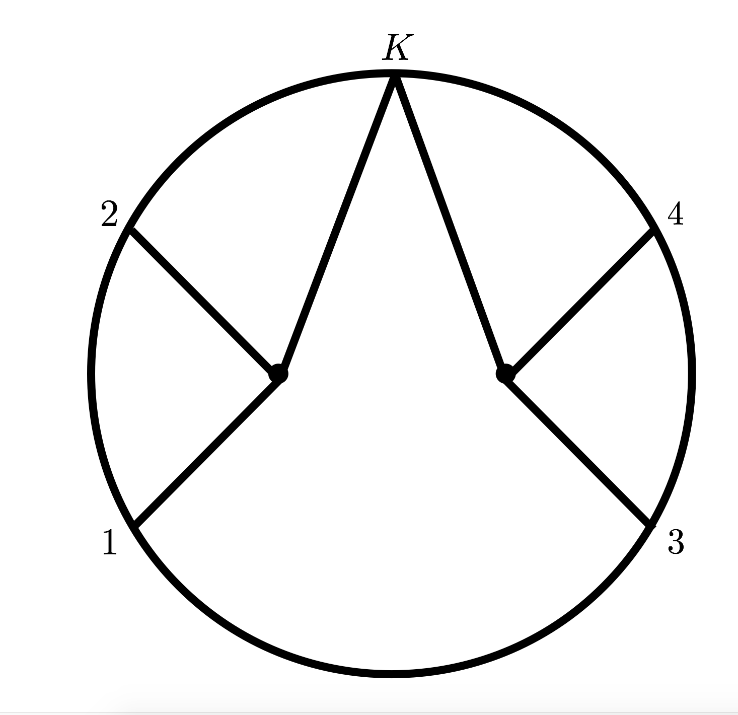
Let us now consider the simple but still not-trivial Witten diagram shown in the figure 1.¹¹ 1 The simplest not trivial diagram corresponds to a 4-point contact diagram., corresponding to a single scalar exchange. We will use this example to illustrate the approach we are going to use in the following over more complicated examples. This diagram was previously computed long time ago in [9] and later revisited in [12] by means of the split-representation which we will review in the appendix A.

Let us recall some few basic facts about Witten diagrams, as the one represented in figure 1. The outer circle represents the boundary of $AdS$. Lines connecting points at the boundary to points in the bulk, represents bulk-to-boundary propagators which are given by

$$G^{\Delta}_{\partial B}(X,P)=\frac{{\cal C}_{\Delta}}{(-2P\cdot X)^{\Delta}},\quad{\cal C}_{\Delta}=\frac{\Gamma(\Delta)}{2\pi^{h}\Gamma(\Delta-h+1)}$$

(2)

where $\Delta$ denotes the conformal dimension of the conformal field at the boundary point $P$. Lines connecting bulk points represents bulk-to-bulk propagators, for which we have choosen the following representation [12],

$$\begin{split}G^{\Delta}_{BB}(X_{1},X_{2})=\int_{-i\infty}^{i\infty}{\mathrm{d}c\,\mathrm{d}\gamma\over(2\pi i)^{2}}{\Gamma(h+c-\gamma)\Gamma(h-c-\gamma)\over\Gamma(c)\Gamma(-c)((\Delta-h)^{2}-c^{2})}{\Gamma(\gamma)\Gamma(h-\gamma)\over\Gamma(2h-2\gamma)\,u^{\gamma}}\,,\end{split}$$

(3)

where $u$ corresponds to the geodesic distance between the points $X_{1}$ and $X_{2}$ and is defined as,

$$u\equiv(X_{1}-X_{2})^{2}=-2(1+X_{1}\cdot X_{2})\,.$$

(4)

Finally, bulk points have to be integrated over. Therefore, the amplitude associated to the diagram represented in figure 1 is given by

$$\begin{split}&{\cal A}^{\mathrlap{\Yright}~\Yleft}_{4}(P_{1},P_{2},P_{3},P_{4})=\\ &g^{2}\int_{AdS}\mathrm{d}X_{1}\mathrm{d}X_{2}G^{\Delta_{1}}_{\partial B}(P_{1},X_{1})G^{\Delta_{2}}_{\partial B}(P_{2},X_{1})G^{\Delta}_{BB}(X_{1},X_{2})G^{\Delta_{3}}_{B\partial}(X_{2},P_{3})G^{\Delta_{4}}_{B\partial}(X_{2},P_{4})\;.\end{split}$$

(5)

where $g$ denotes the coupling of the particles entering the vertex of the diagram (see figure 1). The crucial difference between the approach we are going to use in this note and previous computations (particularly the split representation approach) is that we would like to treat the bulk coordinates $X$ at the same footing as the boundary coordinates $P$. In order to do that, we use the following Mellin-Barnes identity,

$${1\over(A+B)^{\gamma}}={1\over 2\pi i\Gamma(\gamma)}\int_{-i\infty}^{i\infty}\mathrm{d}f\,\Gamma(\gamma+f)\Gamma(-f){A^{f}\over B^{\gamma+f}}\,,$$

(6)

to represent the bulk-to-bulk propagator as,

$$\begin{split}&G^{\Delta}_{BB}(X_{1},X_{2})=\\ &\int_{-i\infty}^{i\infty}{\mathrm{d}c\,\mathrm{d}\gamma\mathrm{d}f\over(2\pi i)^{3}}{\Gamma(h+c-\gamma)\Gamma(h-c-\gamma)\over\Gamma(c)\Gamma(-c)((\Delta-h)^{2}-c^{2})}{\Gamma(\gamma+f)\Gamma(h-\gamma)\Gamma(-f)(-2)^{f}\over\Gamma(2h-2\gamma)\,(-2X_{1}\cdot X_{2})^{\gamma+f}}\\ &\equiv\int_{-i\infty}^{i\infty}{\mathrm{d}c\,\mathrm{d}\gamma\mathrm{d}f\over(2\pi i)^{3}}\,\widehat{G}^{\Delta}_{BB}(c,\gamma,f)\,{1\over(-2X_{1}\cdot X_{2})^{\gamma+f}}\,.\end{split}$$

(7)

For the sake of notation we have defined,

$$\widehat{G}^{\Delta}_{BB}(c,\gamma,f)={\Gamma(h+c-\gamma)\Gamma(h-c-\gamma)\over\Gamma(c)\Gamma(-c)((\Delta-h)^{2}-c^{2})}{\Gamma(\gamma+f)\Gamma(h-\gamma)\Gamma(-f)(-2)^{f}\over\Gamma(2h-2\gamma)}$$

(8)

Putting this definitions back into (5), we get

$$\begin{split}&{\cal A}^{\mathrlap{\Yright}~\Yleft}_{4}(P_{i})=g^{2}\prod_{i=1}^{4}{\cal C}_{\Delta_{i}}\int_{-i\infty}^{i\infty}{\mathrm{d}c\,\mathrm{d}\gamma\mathrm{d}f\over(2\pi i)^{3}}\widehat{G}^{\Delta}_{BB}(c,\gamma,f)\\ &\int_{AdS}{\mathrm{d}X_{1}\mathrm{d}X_{2}\over(-2P_{1}\cdot X_{1})^{\Delta_{1}}(-2P_{2}\cdot X_{1})^{\Delta_{2}}(-2(X_{1}\cdot X_{2}))^{\gamma+f}(-2P_{3}\cdot X_{2})^{\Delta_{3}}(-2P_{4}\cdot X_{2})^{\Delta_{4}}}\,.\end{split}$$

(9)

The first observation from the representation (7) is that it allows to think the amplitudes in the schematic form

$$A\sim\int{\prod\mathrm{d}X_{i}\over(X_{j}\cdot X_{k})^{\Delta_{ij}}(X_{r}\cdot X_{s})^{\Delta_{rs}}}\,,$$

(10)

such us some of the $X_{j}^{\prime}s$ coordinates are projected to the boundary and the remaining should be integrated. We will see also that this representation is convenient when computing the integrals by using Schwinger parametrization. The remaining of the computation proceed similarly as the computation of loop amplitudes in flat space-time. First, we introduce Schwinger parameters to exponentiate all the propagators as,

$$\begin{split}&{\cal A}^{\mathrlap{\Yright}~\Yleft}_{4}(P_{i})=g^{2}\prod_{i=1}^{4}{\cal C}_{\Delta_{i}}\int_{-i\infty}^{i\infty}{\mathrm{d}c\,\mathrm{d}\gamma\mathrm{d}f\over(2\pi i)^{3}}\widehat{G}^{\Delta}_{BB}(c,\gamma,f)\\ &\int^{\infty}_{0}\prod_{i=1}^{5}{\mathrm{d}t_{i}\over t_{i}}{t_{i}^{\Delta_{i}}\over\Gamma(\Delta_{i})}\int_{AdS}\mathrm{d}X_{1}\mathrm{d}X_{2}\,{\rm e}^{2\left(\sum_{i=1}^{2}t_{i}\,P_{i}\cdot X_{1}+t_{5}\,X_{1}\cdot X_{2}+\sum_{i=3}^{4}t_{i}P_{i}\cdot X_{2}\right)}\,.\end{split}$$

(11)

where for convenience of notation we have defined $\Delta_{5}={\gamma+f}$. Integration over bulk coordinates can be carried out straightforwardly now. All of them take the following form,

$$\int\mathrm{d}X_{i}{\rm e}^{2Q_{i}\cdot X_{i}}$$

(12)

which has been computed in [12] and we review here. The key observation is that, since $Q$ is a vector in ${\mathbb{M}}^{d+2}$ and the integral should be Lorenz invariant, we can set $Q=|Q|(1,1,0)$. Then by using the parametrization (1) we can write,

$$\begin{split}\int\mathrm{d}X_{i}{\rm e}^{2Q_{i}\cdot X_{i}}&=\int_{0}^{\infty}{\mathrm{d}z_{i}\over z_{i}}z_{i}^{-d}\int\mathrm{d}^{d}x_{i}\,{\rm e}^{(1+z_{i}^{2}+x_{i}^{2})|Q_{i}|/z}\\ &=\pi^{h}\int_{0}^{\infty}{\mathrm{d}z_{i}\over z_{i}}(z_{i}|Q_{i}|)^{-h}{\rm e}^{(1+z_{i}^{2})|Q_{i}|/z_{i}}\\ &=\pi^{h}\int_{0}^{\infty}{\mathrm{d}z_{i}\over z_{i}}z_{i}^{-h}{\rm e}^{-z_{i}+Q_{i}^{2}/z_{i}}\,,\end{split}$$

(13)

with $h\equiv d/2$. Integration over $X_{1}$ have the form (13) with the corresponding $Q$ given by,

$$Q_{1}=t_{1}P_{1}+t_{2}P_{2}+t_{5}X_{2}\,.$$

(14)

In order to factor out $Q_{1}^{2}$ from the $z_{1}$ integration at the last line of (13), we rescalate $(t_{1},t_{2},t_{5})\to\sqrt{z_{1}}(t_{1},t_{2},t_{5})$ such as ²² 2 Thought as part of the total integral (11).,

$$\begin{split}\int\mathrm{d}X_{1}{\rm e}^{2Q_{1}\cdot X_{1}}&=\pi^{h}{\rm e}^{Q_{1}^{2}}\int_{0}^{\infty}{\mathrm{d}z_{1}\over z_{1}}{\rm e}^{-z_{1}}z_{1}^{\Delta_{1}+\Delta_{2}+\gamma+f-2h\over 2}\\ &={\rm e}^{Q_{1}^{2}}\Gamma\left({\Delta_{1}+\Delta_{2}+\gamma+f-2h\over 2}\right)\,.\end{split}$$

(15)

In the same manner, integration over $X_{2}$ produces an expression as (13) with

$$Q_{2}=t_{1}t_{5}P_{1}+t_{2}t_{5}P_{2}+t_{3}P_{3}+t_{4}P_{4}\,,$$

(16)

and again we re-escalate $(t_{3},t_{4},t_{5})\to\sqrt{z_{2}}(t_{3},t_{4},t_{5})$ to factor out the $Q_{2}$ dependence from the $z_{2}-$integral such as,

$$\begin{split}\int\mathrm{d}X_{2}{\rm e}^{2Q_{2}\cdot X_{2}}&=\pi^{h}{\rm e}^{Q_{2}^{2}}\int_{0}^{\infty}{\mathrm{d}z_{2}\over z_{2}}{\rm e}^{-z_{2}(1+t_{5}^{2})}z_{2}^{\Delta_{3}+\Delta_{4}+\gamma+f-2h\over 2}\\ &={{\rm e}^{Q_{2}^{2}}\over(1+t_{5}^{2})^{\Delta_{3}+\Delta_{4}+\gamma+f-2h\over 2}}\Gamma\left({\Delta_{3}+\Delta_{4}+\gamma+f-2h\over 2}\right)\,.\end{split}$$

(17)

Notice that the term $(1+t_{5}^{2})$ comes from squaring $Q_{2}$, rescaling $z_{2}$ as above and the fact that $X_{3}^{2}=-1$ (or $X_{i}^{2}=-1$ for general bulk points). Later on we will see that those factors coming from the square of the bulk coordinates are the ultimate responsible for the increasing difficulty in performing the integrals at loop level of Witten diagrams on AdS by the Schwinger parametrization approach. This is analogous to the situation in flat space, where theories containing only massless fields $P_{i}^{2}=0$ are much more simpler than massive theories, i.e containing particles such as $X_{i}^{2}=-1$.

After integration over the bulk coordinates, we end up with

$$\begin{split}&{\cal A}^{\mathrlap{\Yright}~\Yleft}_{4}(P_{i})=g^{2}\prod_{i=1}^{4}{\cal C}_{\Delta_{i}}\int_{-i\infty}^{i\infty}{\mathrm{d}c\,\mathrm{d}\gamma\mathrm{d}f\over(2\pi i)^{3}}\widehat{G}^{\Delta}_{BB}(c,\gamma,f)\\ &\int^{\infty}_{0}\prod_{i=1}^{5}{\mathrm{d}t_{i}\over t_{i}}{t_{i}^{\Delta_{i}}\over\Gamma(\Delta_{i})}{1\over(1+t_{5}^{2})^{\Delta_{3}+\Delta_{4}+\gamma+f-2h\over 2}}\Gamma\left({\Delta_{1}+\Delta_{2}+\gamma+f-2h\over 2}\right)\Gamma\left({\Delta_{3}+\Delta_{4}+\gamma+f-2h\over 2}\right)\\ &~~~~{\rm e}^{2(t_{1}t_{2}t_{5}P_{1}\cdot P_{2}+t_{1}t_{3}t_{5}P_{1}\cdot P_{3}+t_{2}t_{3}t_{5}P_{2}\cdot P_{3}+t_{2}t_{4}t_{5}P_{2}\cdot P_{4}+t_{3}t_{4}P_{3}\cdot P_{4})}\,.\end{split}$$

(18)

Now we can use the Symanzik formula [35, 11],

$$\int_{0}^{\infty}\int^{\infty}_{0}\prod_{i=1}^{n}{\mathrm{d}t_{i}\over t_{i}}t_{i}^{\Delta_{i}}{\rm e}^{\sum_{i<j}^{n}t_{i}t_{j}Q_{ij}}={1\over 2(2\pi i)^{n(n-3)\over 2}}\int_{\Sigma_{n}}\prod_{i<j}^{n}\Gamma(\delta_{ij})(Q_{ij})^{-\delta_{ij}}\,,$$

(19)

where $\Sigma_{n}$ is the ${n(n-3)\over 2}-$dimensional Manifold defined by the solution to the system,

$$\delta_{ii}=-\Delta_{i}\,,\quad\sum_{i=1}^{n}\delta_{ij}=0\,.$$

(20)

Using this identity on the integration over the Schwinger parameters associated to the bulk-to-boundary propagators, namely $t_{i}$ with $i\in\{1,\cdots,4\}$, we get,

$$\begin{split}&{\cal A}^{\mathrlap{\Yright}~\Yleft}_{4}(P_{i})=g^{2}\prod_{i=1}^{4}{\cal C}_{\Delta_{i}}\int_{-i\infty}^{i\infty}{\mathrm{d}c\,\mathrm{d}\gamma\mathrm{d}f\over(2\pi i)^{3}}\widehat{G}^{\Delta}_{BB}(c,\gamma,f){1\over 2(2\pi i)^{2}}\int_{\Sigma_{4}}\prod_{i<j}^{4}{\Gamma(\delta_{ij})\over\Gamma(\Delta_{i})}(P_{i}\cdot P_{j})^{-\delta_{ij}}\\ &~~~~~~~~~~~~~\Gamma\left({\Delta_{1}+\Delta_{2}+\gamma+f-2h\over 2}\right)\Gamma\left({\Delta_{3}+\Delta_{4}+\gamma+f-2h\over 2}\right)\\ &~~~~~~~~~~~~~\int^{\infty}_{0}{\mathrm{d}t_{5}\over t_{5}}{t_{5}^{\gamma+f-\delta_{13}-\delta_{14}-\delta_{23}-\delta_{24}}\over\Gamma(\gamma+f)}(1+t_{5}^{2})^{-\delta_{12}-{\Delta_{3}+\Delta_{4}+\gamma+f-2h\over 2}}\end{split}$$

(21)

Integration over $t_{5}$ can be expressed as a beta function and results in,

$$\begin{split}&{\cal A}^{\mathrlap{\Yright}~\Yleft}_{4}(P_{i})=g^{2}\prod_{i=1}^{4}{\cal C}_{\Delta_{i}}\int_{-i\infty}^{i\infty}{\mathrm{d}c\,\mathrm{d}\gamma\mathrm{d}f\over(2\pi i)^{3}}\widehat{G}^{\Delta}_{BB}(c,\gamma,f){1\over 2(2\pi i)^{2}}\int_{\Sigma_{4}}\prod_{i<j}^{4}{\Gamma(\delta_{ij})\over\Gamma(\Delta_{i})}(P_{i}\cdot P_{j})^{-\delta_{ij}}\\ &~~~~~~~~~~\Gamma\left({\Delta_{1}+\Delta_{2}+\gamma+f-2h\over 2}\right)\Gamma\left({\Delta_{3}+\Delta_{4}+\gamma+f-2h\over 2}\right)\\ &~~~~~~~~~~\frac{\Gamma\left(\frac{\gamma+f-\delta_{1,3}-\delta_{1,4}-\delta_{2,3}-\delta_{2,4}}{2}\right)\Gamma\left(\frac{-2h+2\delta_{1,2}+\delta_{1,3}+\delta_{1,4}+\delta_{2,3}+\delta_{2,4}+\Delta(3)+\Delta(4)}{2}\right)}{2\Gamma\left(-h+\delta_{1,2}+\frac{\gamma+f+\Delta(3)+\Delta(4)}{2}\right)}\,,\end{split}$$

(22)

also the integration over $f$ can be performed straightforwardly leading to

$$\begin{split}&{\cal A}^{\mathrlap{\Yright}~\Yleft}_{4}(P_{i})={1\over 2(2\pi i)^{2}}\int_{\Sigma_{4}}\prod_{i<j}^{4}{\Gamma(\delta_{ij})\over\Gamma(\Delta_{i})}(P_{i}\cdot P_{j})^{-\delta_{ij}}\\ &\times\,g^{2}\prod_{i=1}^{4}{\cal C}_{\Delta_{i}}\int_{-i\infty}^{i\infty}{\mathrm{d}c\,\mathrm{d}\gamma\over(2\pi i)^{2}}{\Gamma(h+c-\gamma)\Gamma(h-c-\gamma)\over\Gamma(c)\Gamma(-c)((\Delta-h)^{2}-c^{2})}{\Gamma(h-\gamma)\over\Gamma(2h-2\gamma)}\\ &~~\times\,\frac{\Gamma\left(\frac{\gamma-s}{2}\right)\Gamma\left(\frac{-2h+\gamma+\Delta_{1}+\Delta_{2}}{2}\right)\Gamma\left(\frac{-2h+\gamma+\Delta_{3}+\Delta_{4}}{2}\right)}{\Gamma\left(\frac{-s+\Delta_{1}+\Delta_{2}}{2}\right)\Gamma\left(\frac{-s+\Delta_{3}+\Delta_{4}}{2}\right)}\,.\end{split}$$

(23)

Where $s$ and $t$ are defined by the following solutions of the system (20) for $n=4$,

$$\begin{split}\delta_{12}&=\frac{1}{2}\left(\Delta_{1}+\Delta_{2}-s\right)\,,\quad\delta_{13}=\frac{1}{2}\left(\Delta_{1}+\Delta_{3}-t\right)\,,\\ \delta_{14}&=\frac{1}{2}\left(-\Delta_{2}-\Delta_{3}+s+t\right)\,,\quad\delta_{23}=\frac{1}{2}\left(-\Delta_{1}-\Delta_{4}+s+t\right)\,,\\ \delta_{24}&=\frac{1}{2}\left(\Delta_{2}+\Delta_{4}-t\right)\,,\quad\delta_{34}=\frac{1}{2}\left(\Delta_{3}+\Delta_{4}-s\right)\,.\end{split}$$

(24)

Following Mack [11] and knowing that Witten diagrams correspond to correlation functions on the boundary (or pieces of the whole correlator), we expect the following Mellin representation,

$$A(P_{i})={{\cal N}\over(2\pi i)^{n(n-3)\over 2}}\int_{\Sigma_{n}}\mathrm{d}\delta_{ij}M(\delta_{ij})\prod_{i<j}^{n}\Gamma(\delta_{ij})(P_{i}\cdot P_{j})^{-\delta_{ij}}\,,$$

(25)

with

$${\cal N}={1\over 2}\Gamma\left({\sum_{i=1}^{n}\Delta_{i}-2h\over 2}\right)\prod_{i=1}^{n}{{\cal C}_{\Delta_{i}}\over\Gamma(\Delta_{i})}$$

(26)

therefore comparing with (23) we conclude that the Mellin amplitude for the exchaged scalar diagram can be represented by ³³ 3 In this case the Mellin amplitude does not depend on $t$ because we are considering only the $s-$channel exchange.,

$$\begin{split}&M^{\mathrlap{\Yright}~\Yleft}=g^{2}\int_{-i\infty}^{i\infty}{\mathrm{d}c\,\mathrm{d}\gamma\over(2\pi i)^{2}}{\Gamma(h+c-\gamma)\Gamma(h-c-\gamma)\over\Gamma(c)\Gamma(-c)((\Delta-h)^{2}-c^{2})}{\Gamma(h-\gamma)\over\Gamma(2h-2\gamma)}\\ &~~\frac{\Gamma\left(\frac{\gamma-s}{2}\right)\Gamma\left(\frac{-2h+\gamma+\Delta_{1}+\Delta_{2}}{2}\right)\Gamma\left(\frac{-2h+\gamma+\Delta_{3}+\Delta_{4}}{2}\right)}{\Gamma\left(\frac{-2h+\Delta_{1}+\Delta_{2}+\Delta_{3}+\Delta_{4}}{2}\right)\Gamma\left(\frac{-s+\Delta_{1}+\Delta_{2}}{2}\right)\Gamma\left(\frac{-s+\Delta_{3}+\Delta_{4}}{2}\right)}\,.\end{split}$$

(27)

The bubble Witten diagram corresponds to a similar expression as (5) but with two bulk-to-bulk propagators connecting the same points $X_{1},\,X_{2}$ instead of one, as shown in figure 2. In practice, we can think of the product of the two bulk-to-bulk propagators that depend on the same $u$, as a single bulk-to-bulk propagator of the form (3) but with two $c-$integrations and two $\gamma-$integrations. That particularity allow us to do a single expansion of the type (6) on the product, instead of one for each propagator. The amplitude associated to this diagram is given by

$$\begin{split}&{\cal A}^{\mathrlap{\vee}\wedge}_{4}(P_{1},P_{2},P_{3},P_{4})=\\ &g^{2}\int_{AdS}\mathrm{d}X_{1}\mathrm{d}X_{2}G^{\Delta_{1}}_{\partial B}(P_{1},X_{1})G^{\Delta_{2}}_{\partial B}(P_{2},X_{2})G^{\Delta}_{BB}(X_{1},X_{2})G^{\Delta^{\prime}}_{BB}(X_{1},X_{2})G^{\Delta_{3}}_{B\partial}(X_{2},P_{3})G^{\Delta_{4}}_{B\partial}(X_{2},P_{4})\;.\end{split}$$

(28)

Replacing the definitions for the bulk-to-boundary propagators, the representation (3) and using (6) we get,

$$\begin{split}&{\cal A}^{\mathrlap{\vee}\wedge}_{4}(P_{i})=g^{2}\prod_{i=1}^{4}{\cal C}_{\Delta_{i}}\prod_{j=1}^{2}\int_{-i\infty}^{i\infty}{\mathrm{d}c_{j}\,\mathrm{d}\gamma_{j}\mathrm{d}f\over(2\pi i)^{4}}\\ &{\Gamma(h+c_{j}-\gamma_{j})\Gamma(h-c_{j}-\gamma_{j})\Gamma(\gamma_{j})\Gamma(h-\gamma_{j})\over\Gamma(c_{j})\Gamma(-c_{j})((\Delta-h)^{2}-c_{1}^{2})((\Delta^{\prime}-h)^{2}-c_{2}^{2})\Gamma(2h-2\gamma_{j})}{\Gamma(\gamma_{1}+\gamma_{2}+f)\Gamma(-f)(-2)^{f}\over\Gamma(\gamma_{1}+\gamma_{2})}\\ &\int_{AdS}{\mathrm{d}X_{1}\mathrm{d}X_{2}\over(-2P_{1}\cdot X_{1})^{\Delta_{1}}(-2P_{2}\cdot X_{1})^{\Delta_{2}}(-2(X_{1}\cdot X_{2}))^{\gamma_{j}+f_{j}}(-2P_{3}\cdot X_{2})^{\Delta_{3}}(-2P_{4}\cdot X_{2})^{\Delta_{4}}}\,.\end{split}$$

(29)

we can notice that the computation should follows the same lines as the exchange diagram in section above with $\Delta_{5}$ in (11) replaced by $\Delta_{5}=\gamma_{1}+\gamma_{2}+f$, leading us to the following representation of the corresponding Mellin amplitude,

$$\begin{split}&M^{\mathrlap{\vee}\wedge}_{4}=g^{2}\prod_{j=1}^{2}\int_{-i\infty}^{i\infty}{\mathrm{d}c_{j}\,\mathrm{d}\gamma_{j}\over(2\pi i)^{4}}\\ &{\Gamma(h+c_{j}-\gamma_{j})\Gamma(h-c_{j}-\gamma_{j})\Gamma(\gamma_{j})\Gamma(h-\gamma_{j})\over\Gamma(c_{j})\Gamma(-c_{j})((\Delta-h)^{2}-c_{1}^{2})((\Delta^{\prime}-h)^{2}-c_{2}^{2})\Gamma(2h-2\gamma_{j})}{1\over\Gamma(\gamma_{1}+\gamma_{2})}\\ &~~\frac{\Gamma\left(\frac{\gamma_{1}+\gamma_{2}-s}{2}\right)\Gamma\left(\frac{-2h+\gamma_{1}+\gamma_{2}+\Delta_{1}+\Delta_{2}}{2}\right)\Gamma\left(\frac{-2h+\gamma_{1}+\gamma_{2}+\Delta_{3}+\Delta_{4}}{2}\right)}{\Gamma\left(\frac{-2h+\Delta_{1}+\Delta_{2}+\Delta_{3}+\Delta_{4}}{2}\right)\Gamma\left(\frac{-s+\Delta_{1}+\Delta_{2}}{2}\right)\Gamma\left(\frac{-s+\Delta_{3}+\Delta_{4}}{2}\right)}\,.\end{split}$$

(30)

Before moving onto the remaining loop corrections to the four point scattering amplitude, let us consider the one-loop correction to the three point function, represented in figure 3 and given by,

$${\cal A}^{\rhd}_{3}(P_{i})=g^{3}\prod_{i=1}^{3\,{\rm Mod}3}\int_{AdS}\mathrm{d}X_{i}\,G^{\Delta_{i}}_{\partial B}(P_{i},X_{i})G^{\Delta_{ii+1}}_{BB}(X_{i},X_{i+1})\,.$$

(31)

Introducing Schwinger parameters in the usual way we have,

$$\begin{split}&{\cal A}^{\rhd}_{3}(P_{i})=g^{3}\prod_{i=1}^{3\,{\rm Mod}3}\,\widehat{G}^{\Delta_{ii+1}}_{BB}(c_{i,i+1},\,\gamma_{i,i+1},\,f_{i,i+1})\\ &~~~~\times\prod_{j=1}^{7}\int_{0}^{\infty}{\mathrm{d}t_{j}\over t_{j}\,\Gamma(\Delta_{j})}t_{j}^{\Delta_{j}}\int_{AdS}\mathrm{d}X_{i}{\rm e}^{2(t_{1}P_{1}+t_{5}X_{2}+t_{7}X_{3})\cdot X_{1}}{\rm e}^{2(t_{2}P_{2}+t_{6}X_{3})\cdot X_{2}}{\rm e}^{2(t_{3}P_{3})\cdot X_{3}}\,,\end{split}$$

(32)

where we have redefined the conformal weights of the bulk-to-bulk propagators in (31) as $\Delta_{5}\equiv\Delta_{12}=\gamma_{12}+f_{12},\,~\Delta_{6}\equiv\Delta_{23}=\gamma_{23}+f_{23},\,~\Delta_{7}\equiv\Delta_{13}=\gamma_{31}+f_{31}$. We then proceed to integrate the bulk coordinates in the exact same manner as in the previous cases to get

$$\begin{split}&{\cal M}^{\rhd}_{3}(P_{i})=\prod_{i=1}^{3\,{\rm Mod}3}\int_{-i\infty}^{i\infty}{\mathrm{d}c_{i\,i+1}\,\mathrm{d}\gamma_{i\,i+1}\mathrm{d}f_{i\,i+1}\over(2\pi i)^{4}}{\Gamma(h+c_{i\,i+1}-\gamma_{i\,i+1})\Gamma(h-c_{i\,i+1}-\gamma_{i\,i+1})\over\Gamma(c_{i\,i+1})\Gamma(-c_{i\,i+1})((\Delta-h)^{2}-c_{i\,i+1}^{2})}\\ &{\Gamma(h-\gamma_{i\,i+1})\Gamma(-f_{i\,i+1})(-2)^{f}_{i\,i+1}\over\Gamma(2h-2\gamma_{i\,i+1})}\\ &\Gamma\left({\Delta_{1}+\gamma_{12}+f_{12}+\gamma_{31}+f_{31}-2h\over 2}\right)\Gamma\left({\Delta_{2}+\gamma_{12}+f_{12}+\gamma_{23}+f_{23}-2h\over 2}\right)\\ &\Gamma\left({\Delta_{3}+\gamma_{23}+f_{23}+\gamma_{31}+f_{31}-2h\over 2}\right)\\ &\prod_{j=5}^{7}\int{\mathrm{d}t_{j}\over t_{j}}\,t_{j}^{\Delta_{j}}\,{T_{7}^{-\delta_{12}}\,T_{6}^{-\delta_{13}}\,T_{5}^{-\delta_{23}}\,(1+t_{7}^{2}+T_{5}^{2})^{-{\Delta_{3}+\gamma_{23}+f_{23}+\gamma_{31}+f_{31}-2h\over 2}}\over(1+t_{5}^{2})^{{\Delta_{2}+\gamma_{12}+f_{12}+\gamma_{23}+f_{23}-2h\over 2}}}\end{split}$$

(33)

where for convenience of notation we have defined $T_{5}=t_{5}t_{7}+t_{6},\,T_{6}=t_{5}T_{5}+t_{7},\,T_{7}=T_{6}T_{5}$. Notice that in this case, the Mellin amplitude does not depend on any kinematical degrees of freedom, or in other words it is just a constant, since the solution of the system of equation (20) is simply,

$$\delta_{12}={\Delta_{1}+\Delta_{2}-\Delta_{3}\over 2},\,~\delta_{13}={\Delta_{1}+\Delta_{3}-\Delta_{2}\over 2},\,~\delta_{23}={\Delta_{2}+\Delta_{3}-\Delta_{1}\over 2}\,.$$

(34)

This is just the reflection of the fact that the three-point function is fixed by conformal invariance up to a constant, so what we are really computing here is the loop correction of the three point structure constant.

Let us focus now on the integral on the last line of (33),

$$\begin{split}&\int{\mathrm{d}t_{5}\over t_{5}}{\mathrm{d}T_{5}}{\mathrm{d}t_{7}\over t_{7}}\,t_{5}^{\Delta_{5}}(T_{5}-t_{5}t_{7})^{\Delta_{6}-1}\,t_{7}^{\Delta_{7}}\,\\ &\times{(t_{5}T_{5}+t_{7})^{-\delta_{12}-\delta_{13}}\,T_{5}^{-\delta_{12}-\delta_{23}}\,(1+t_{7}^{2}+T_{5}^{2})^{-{\Delta_{3}+\gamma_{23}+f_{23}+\gamma_{31}+f_{31}-2h\over 2}}\over(1+t_{5}^{2})^{{\Delta_{2}+\gamma_{12}+f_{12}+\gamma_{23}+f_{23}-2h\over 2}}}\end{split}$$

(35)

where we have replaced $t_{6}$ by $T_{5}$. This looks like a difficult integral to perform, let alone in a clean compact way, so we choose at this point to perform a brute force approach. In order to do so, we expand the factor $(1+t_{7}^{2}+T_{5}^{2})$ in the numerator (35) by means of applying the Mellin-Barnes transform (6) one more time,

$$\begin{split}&\int_{-i\infty}^{i\infty}{\mathrm{d}\ell\over 2\pi i}{\Gamma(a+\ell)\Gamma(-\ell)\over\Gamma(a)}I^{\rhd}_{S}\,,\end{split}$$

(36)

where we have defined the new integral,

$$I^{\rhd}_{S}\equiv\int{\mathrm{d}t_{5}\over t_{5}}{\mathrm{d}T_{5}}{\mathrm{d}t_{7}\over t_{7}}\,t_{5}^{\Delta_{5}}(T_{5}-t_{5}t_{7})^{\Delta_{6}-1}\,t_{7}^{\Delta_{7}}{(t_{5}T_{5}+t_{7})^{-\delta_{12}-\delta_{13}}\,T_{5}^{2\ell-\delta_{12}-\delta_{23}}\over(1+t_{5}^{2})^{b}(1+t_{7}^{2})^{a+\ell}}$$

(37)

and $a={{\Delta_{3}+\gamma_{23}+f_{23}+\gamma_{31}+f_{31}-2h\over 2}}$, $b={\Delta_{2}+\gamma_{12}+f_{12}+\gamma_{23}+f_{23}-2h\over 2}$. With the help of Mathematica [36] this expansion allow us to represent the integral over all the remaining Schwinger parameters in terms of a lengthy combination of Hypergeometric functions, as is shown in Appendix equation (80). However, we will discuss an approach to deal with a more general family of integrals in section 7 which includes the one above.

References

- (1) J. M. Maldacena, The Large N limit of superconformal field theories and supergravity, Int. J. Theor. Phys. 38 (1999) 1113–1133, [hep-th/9711200].
- (2) E. Witten, Anti-de Sitter space and holography, Adv. Theor. Math. Phys. 2 (1998) 253–291, [hep-th/9802150].
- (3) S. Pasterski, S.-H. Shao and A. Strominger, Flat Space Amplitudes and Conformal Symmetry of the Celestial Sphere, 1701.00049.
- (4) C. Cardona and Y.-t. Huang, S-matrix singularities and CFT correlation functions, 1702.03283.
- (5) G. Arutyunov, F. A. Dolan, H. Osborn and E. Sokatchev, Correlation functions and massive Kaluza-Klein modes in the AdS / CFT correspondence, Nucl. Phys. B665 (2003) 273–324, [hep-th/0212116].
- (6) D. Z. Freedman, S. D. Mathur, A. Matusis and L. Rastelli, Comments on 4 point functions in the CFT / AdS correspondence, Phys. Lett. B452 (1999) 61–68, [hep-th/9808006].
- (7) H. Liu and A. A. Tseytlin, On four point functions in the CFT / AdS correspondence, Phys. Rev. D59 (1999) 086002, [hep-th/9807097].
- (8) W. Mueck and K. S. Viswanathan, Conformal field theory correlators from classical scalar field theory on AdS(d+1), Phys. Rev. D58 (1998) 041901, [hep-th/9804035].
- (9) E. D’Hoker, D. Z. Freedman, S. D. Mathur, A. Matusis and L. Rastelli, Graviton exchange and complete four point functions in the AdS / CFT correspondence, Nucl. Phys. B562 (1999) 353–394, [hep-th/9903196].
- (10) F. A. Dolan and H. Osborn, Implications of N=1 superconformal symmetry for chiral fields, Nucl. Phys. B593 (2001) 599–633, [hep-th/0006098].
- (11) G. Mack, D-independent representation of Conformal Field Theories in D dimensions via transformation to auxiliary Dual Resonance Models. Scalar amplitudes, 0907.2407.
- (12) J. Penedones, Writing CFT correlation functions as AdS scattering amplitudes, JHEP 03 (2011) 025, [1011.1485].
- (13) A. L. Fitzpatrick, J. Kaplan, J. Penedones, S. Raju and B. C. van Rees, A Natural Language for AdS/CFT Correlators, JHEP 11 (2011) 095, [1107.1499].
- (14) E. Hijano, P. Kraus, E. Perlmutter and R. Snively, Witten Diagrams Revisited: The AdS Geometry of Conformal Blocks, JHEP 01 (2016) 146, [1508.00501].
- (15) E. Dyer, D. Z. Freedman and J. Sully, Spinning Geodesic Witten Diagrams, 1702.06139.
- (16) C. Sleight and M. Taronna, Spinning Witten Diagrams, JHEP 06 (2017) 100, [1702.08619].
- (17) H.-Y. Chen, E.-J. Kuo and H. Kyono, Anatomy of Geodesic Witten Diagrams, JHEP 05 (2017) 070, [1702.08818].
- (18) A. Castro, E. Llabrés and F. Rejon-Barrera, Geodesic Diagrams, Gravitational Interactions & OPE Structures, JHEP 06 (2017) 099, [1702.06128].
- (19) M. Nishida and K. Tamaoka, Geodesic Witten diagrams with an external spinning field, PTEP 2017 (2017) 053B06, [1609.04563].
- (20) A. L. Fitzpatrick and J. Kaplan, Unitarity and the Holographic S-Matrix, JHEP 10 (2012) 032, [1112.4845].
- (21) A. L. Fitzpatrick and J. Kaplan, Analyticity and the Holographic S-Matrix, JHEP 10 (2012) 127, [1111.6972].
- (22) L. Cornalba, M. S. Costa and J. Penedones, Eikonal approximation in AdS/CFT: Resumming the gravitational loop expansion, JHEP 09 (2007) 037, [0707.0120].
- (23) A. A. Nizami, A. Rudra, S. Sarkar and M. Verma, Exploring Perturbative Conformal Field Theory in Mellin space, JHEP 01 (2017) 102, [1607.07334].
- (24) L. F. Alday, Large Spin Perturbation Theory, 1611.01500.
- (25) S. Caron-Huot, Analyticity in Spin in Conformal Theories, 1703.00278.
- (26) D. Simmons-Duffin, The Lightcone Bootstrap and the Spectrum of the 3d Ising CFT, JHEP 03 (2017) 086, [1612.08471].
- (27) L. F. Alday and A. Bissi, Loop Corrections to Supergravity on , 1706.02388.
- (28) O. Aharony, L. F. Alday, A. Bissi and E. Perlmutter, Loops in AdS from Conformal Field Theory, JHEP 07 (2017) 036, [1612.03891].
- (29) F. Aprile, J. M. Drummond, P. Heslop and H. Paul, Quantum Gravity from Conformal Field Theory, 1706.02822.
- (30) D. Li, D. Meltzer and D. Poland, Conformal Bootstrap in the Regge Limit, 1705.03453.
- (31) M. S. Costa, T. Hansen and J. Penedones, Bounds for OPE coefficients on the Regge trajectory, 1707.07689.
- (32) S. Giombi, C. Sleight and M. Taronna, Spinning AdS Loop Diagrams: Two Point Functions, 1708.08404.
- (33) P. A. M. Dirac, Wave equations in conformal space, Annals Math. 37 (1936) 429–442.
- (34) J. Penedones, High Energy Scattering in the AdS/CFT Correspondence. PhD thesis, Porto U., 2007. 0712.0802.
- (35) K. Symanzik, On Calculations in conformal invariant field theories, Lett. Nuovo Cim. 3 (1972) 734–738.
- (36) W. R. Inc., “Mathematica, Version 11.1.”
- (37) N. Arkani-Hamed, J. Bourjaily, F. Cachazo and J. Trnka, Unification of Residues and Grassmannian Dualities, JHEP 01 (2011) 049, [0912.4912].
- (38) P. Griffiths and H. Harris, Principles of Algebraic Geometry, Wiley Classics Library Edition (1994) .
- (39) E. Cattani, A. Dickenstein and B. Sturmfels, Computing Multidimensional Residues, .
- (40) C. Cardona and C. Kalousios, Elimination and recursions in the scattering equations, Phys. Lett. B756 (2016) 180–187, [1511.05915].
- (41) L. Dolan and P. Goddard, General Solution of the Scattering Equations, JHEP 10 (2016) 149, [1511.09441].
- (42) C. Cardona and C. Kalousios, Comments on the evaluation of massless scattering, JHEP 01 (2016) 178, [1509.08908].
- (43) A. Dickenstein and I. Emiris, Multihomogeneous resultant matrices, ISSAC 2002 (2002) .
- (44) I.M. Gelfand, M.M. Kapranov, A.V. Zelevinsky, Discriminants, Resultants, and Multidimensional Determinants, (Birkhäuser, Boston, 1994) .
- (45) B. Sturmfels, Solving Systems of Polynomial Equations, Cbms Regional Conference Series in Mathematics. American Mathematical Society (2002) .
- (46) N. Arkani-Hamed, J. L. Bourjaily, F. Cachazo, A. B. Goncharov, A. Postnikov and J. Trnka, Grassmannian Geometry of Scattering Amplitudes. Cambridge University Press, 2016.
- (47) F. Cachazo, S. He and E. Y. Yuan, Scattering of Massless Particles in Arbitrary Dimensions, Phys. Rev. Lett. 113 (2014) 171601, [1307.2199].
- (48) M. S. Costa, V. Gonçalves and J. Penedones, Spinning AdS Propagators, JHEP 09 (2014) 064, [1404.5625].
- (49) D. Z. Freedman, S. D. Mathur, A. Matusis and L. Rastelli, Correlation functions in the CFT(d) / AdS(d+1) correspondence, Nucl. Phys. B546 (1999) 96–118, [hep-th/9804058].