Sparse polynomial interpolation: sparse recovery, super resolution, or Prony?
Abstract
We show that the sparse polynomial interpolation problem reduces to a discrete super-resolution problem on the -dimensional torus. Therefore the semidefinite programming approach initiated by Candès & Fernandez-Granda [7] in the univariate case can be applied. We extend their result to the multivariate case, i.e., we show that exact recovery is guaranteed provided that a geometric spacing condition on the supports holds and the number of evaluations are sufficiently many (but not many). It also turns out that the sparse recovery LP-formulation of -norm minimization is also guaranteed to provide exact recovery provided that the evaluations are made in a certain manner and even though the Restricted Isometry Property for exact recovery is not satisfied. (A naive sparse recovery LP-approach does not offer such a guarantee.) Finally we also describe the algebraic Prony method for sparse interpolation, which also recovers the exact decomposition but from less point evaluations and with no geometric spacing condition. We provide two sets of numerical experiments, one in which the super-resolution technique and Prony’s method seem to cope equally well with noise, and another in which the super-resolution technique seems to cope with noise better than Prony’s method, at the cost of an extra computational burden (i.e. a semidefinite optimization).
Keywords:
Linear programming Prony’s method Semidefinite programming super-resolution1 Introduction
In many domains, functions can be described in a way which is easy to evaluate, but not necessarily easy to identify. This can be the case when the function comes from the analysis of the input-ouput response of a complex system or from an algorithmic construction. Interpolation strategies have shown to be very effective in the reconstruction of such black-box functions, in particular in computer algebra, for sparse multivariate polynomials. Such black-box polynomials may be built with “approximate” coefficients, so that the evaluation at a point may be an approximate value with error or noise. While efficient exact methods exist for the interpolation of sparse polynomials, interpolation of approximate sparse multivariate polynomials remains a challenging problem.
A motivation of this work is to show that the sparse interpolation problem can be solved exactly under some conditions of separability of the support, by three different methods following different perspectives. One of them is a direct algebraic method and the two others are based on convex optimization tools (LP, SDP). We analyze them in detail and investigate their numerical robustness and their efficiency to address the interpolation problem of black-box sparse multivariate polynomials.
Suppose that we are given a black-box polynomial , that is, is unknown but given any “input” point , the black-box outputs the complex number . We assume that the polynomial is sparse, that is, it has only a few number of non-zero terms, compared to the number of monomials of degree less or equal to the degree of . Sparse interpolation is concerned with recovering the unknown monomials and coefficients of a sparse polynomial in a way, which depends on the number of non-zero terms of . In the sole knowledge of a few (and as few as possible) values of at some points that one may choose at our convenience, one want to recover the non-zero terms of the polynomial .
Hereafter, we present three families of methods for robust sparse interpolation, using either direct algebraic computation or convex optimization. Direct algebraic methods shall compute sparse representation using a minimal number of values. Convex optimization techniques shall help improving robustness, in the presence of numerical errors. All of these methods allow to choose the points of evaluation.
Prony
The method goes back to the pioneer work of G. R de Prony [13] who was interested in recovering a sum of few exponential terms from sampled values of the function. Thus Prony’s method is also a standard tool to recover a complex atomic measure from knowledge of some of its moments [28]. Briefly, in the univariate setting this purely algebraic method consists of two steps: (i) Computing the coefficients of a polynomial whose roots form the finite support of the unknown measure. As satisfies a recurrence relation it is the unique element (up to scaling) in the kernel of a (Hankel) matrix. (ii) The weights associated to the atoms of the support solve a Vandermonde system.
This algebraic method has then been used in the context of sparse polynomial interpolation. In the univariate case it consists in evaluating the black-box polynomial at values of the form for a finite number of pairs , fixed. A sequence of evaluations allows to recover the decomposition exactly, where is the number of terms of the sparse polynomial. The decomposition is obtained by computing a minimal recurrence relation between these evaluations, by finding the roots of the associate polynomial, which yields the exponents of the monomials and by solving a Vandermonde system which yields the coefficients of the terms in the sparse polynomial.
Since then, it has been extended to address numerical issues and to treat applications in various domains, particularly in signal processing. Methods such as MUSIC, ESPRIT extend the initial method of Prony, by adding robust numerical linear algebra ingredients. See e.g. [36], [40], [20], [4], [35], [34] and the many references therein.
The approach is closely related to sparse Fast Fourier Transform techniques, where evaluations at powers of the -th root of unity are used to recover a -sparse signal. The bounds, in the univariate case, on the number of samples and runtime complexity are linear in up to polylog factors in or . See e.g. [9], [23].
From an algorithmic point of view, the approach has been improved by exploiting the Berlekamp-Massey algorithm [3], [30] and the structure of the involved matrices; see e.g. [25], [42], [21].
Prony’s approach has also been applied to treat multivariate sparse interpolation problems [41] and [2], by evaluation at points with coordinates in geometric progressions. It has also been extended to approximate data [19], using the same type of point evaluation sequences. It has been applied to sparse polynomial interpolation with noisy data in [44] to provide a way to recover a blackbox univariate polynomial exactly when some (but not all) of its evaluations are corrupted with noise (in the sipirit of error-decoding).
Generalizations of Prony’s method to multivariate reconstruction problems have been developed more recently. In [28], a projection based method is used to compute univariate polynomials which roots determine the coordinates of the terms in the sparse representation. In [38], an -basis of the kernel ideal of a moment matrix is computed and used to find the roots which determine the sparse decomposition. Direct decomposition methods which compute the algebraic structure of the Artinian Gorenstein algebra associated to the moment matrix and deduce the sparse representation from eigenvectors of multiplication operators are developed in [31] and [22].
Sparse recovery
“Sparse recovery” refers to methods for estimating a sparse representation from solutions of underdetermined linear systems. It corresponds to the mathematical aspects of what is know as “Compressed sensing” in Signal Processing. Here we consider a naive “sparse recovery” LP-approach, which consists of solving where is the vector of coefficients of the unknown polynomial and are linear constraints obtained from evaluations at some given points. By minimizing the norm one expects to obtain a “sparse” solution to the undetermined system . However since the matrix does not satisfy the sufficient Restricted Isometry Property (RIP), exact recovery is not guaranteed (at least by invoking results from compressed sensing). Only probabilistic results may be expected in the univariate case if enough sampling points (of the order where is number of non-zero terms, is the maximal degree of the terms and is a constant measuring the coherence of ) are chosen at random, as in [8].
Super-resolution
Super-resolution refers to techniques to enhancing the resolution of sensing systems. In [7], it refers to the process or retrieving fine scale structures from coarse scale information, such as Fourier coefficients. In more mathematical terms, it consists in recovering the support of a sparse atomic (signed) measure on a compact set , from known moments. Hereafter we will consider the particular case where is the multi-dimensional torus . In the work of Candès and Fernandez-Granda [7] it is shown that if the support atoms of the measure are well-separated then the measure is the unique solution of an infinite-dimensional convex optimization problem on a space of measures with the total variation as minimization criterion. In the univariate case its (truncated) moment matrix can be recovered by solving a single Semidefinite Program (SDP). The number of evaluations needed for exact recovery is then at most if is the number of atoms11 1 As noted in Candès and Fernandez-Granda [7], with the proviso that the number of evaluations is larger than 128 (and in fact significantly less in all numerical examples provided). Interestingly, the total-variation minimization technique adapts nicely to noisy model and yields stable approximations of the weighted sum of Dirac measures, provided that the support atoms are well separated, see e.g. [6], [1], [17].
An extension to the multivariate case has been proposed in [15] to recover weight sums of Dirac measures in , where now one needs to solve a hierarchy of semidefinite programs.
The existence and unicity of the solution of the total variation minimization problem relies on the existence of a dual certificate, that is, a polynomial with -norm reached at the points of the support of the measure. The relaxation into a hierarchy of semidefinite programs [15] yields a decomposition into a finite weighted sum of Dirac measures, provided that at some order of the hierarchy, a flat extension condition is satisfied at an optimal solution. Then the decomposition can be recovered from the moment matrix at this optimal solution by applying a Prony’s like technique.
Contribution
We propose a new multivariate variant of Prony’s method for sparse polynomial interpolation, which avoids projections in one variables and requires a small number of evaluations. In particular, it differs from approaches such as [19], which uses special “aligned” moments to apply Prony univariate method. In the univariate case, the new method only requires evaluations (instead of ) where is the number of monomials of the blackbox polynomial. Similarly in the multivariate case, we show that the number of needed evaluations is significantly reduced. It involves a Toeplitz matrix rather than a Hankel matrix. Numerical experiments confirm the theoretical result regarding the number of evaluations and robustness against perturbations. This new multivariate Toeplitz-Prony can be seen as an extension of ESPRIT methods in several variables. As stated in [39][p.167], ESPRIT should be preferred to MUSIC for frequency estimation in signal processing. The numerical experiments corroborate this claim by showing the good numerical behavior of the new multivariate Toeplitz-Prony method.
We consider the naive sparse recovery approach to sparse interpolation via -norm minimization and we characterize optimal solutions via standard arguments of linear programming (LP). Interestingly, this characterization is a “formal analogue” in appropriate spaces of that in super-resolution (2.1) in some measure spaces. However as the matrix does not satisfy the RIP there is no guarantee (at least by invoking results from compressed sensing) that an optimal solution is unique and corresponds to the unique sparse black-box polynomial .
We then propose another approach which uses the fact that one has the choice of points at which evaluations of can be done through the black-box and yields the following simple but crucial observation: By choosing as some power with (and where is fixed, arbitrary) the sparse polynomial can be viewed as a signed atomic measure on with finitely many atoms associated with the nonzero coefficients of (the signed weights of associated with each atom). In doing so the sparse interpolation problem is completely equivalent to a super-resolution problem on the multi-dimensional torus . We prove a new unicity theorem (Theorem 3.4) for the optimal solution of the super-resolution problem on , provided enough moments of the measure are known. Namely, if where is the interpolation entropy of the support of a measure on and , we show that the super-resolution optimisation problem with all the moments of -degree of the measure has a unique solution (i.e. ). This result is non trivial extension to any dimension of Theorems 1.2, 1.3 in Candès and Fernandez-Granda [7] proved for one and two variables. Consequently, the sparse polynomial is the unique optimal solution of a certain infinite-dimensional linear program on a space of measures, provided that a geometric condition of minimum spacing (between atoms of the support) is satisfied and sufficiently many evaluations are available. Notice that previous works on Prony’s method (e.g. [44]) have also exploited (but in a different manner) evaluations at consecutive powers of a fixed element. In fact our view of a polynomial as a signed atomic measure on the torus is probably the shortest way to explain why Prony’s method can be used for polynomial interpolation (as the original Prony’s method can be interpreted directly as reconstructing an atomic measure on the complex plane from some of its moments [28]).
We then relax this problem to a new hierarchy of semidefinite programs. This hierarchy requires less moments or evaluations than a degree-based moment relaxation. In principle, the convergence is only asymptotic (and guaranteed to be finite only in the cases ). However generic finite convergence results of polynomial optimization of [33] seem to be also valid in our context as evidenced from our numerical experiments (and in those in De Castro et al. [15] in signal processing). The flat extension rank condition on moment matrices of Curto and Fialkow (12, Theorem 1.1) or its generalization in [29] can be extended to Toeplitz-like moment matrices [24], to test whether finite convergence takes place. In all our numerical experiments, finite convergence takes place and the coefficients and exponents of the unknown polynomial could be extracted. To give an idea, a univariate polynomial of degree with 3 atoms can be recovered by solving a single SDP with associated Toeplitz matrices and which only involves evaluations. On the other hand if some atoms are close to each other then more information (i.e. evaluations) is needed as predicted by the spacing condition (and confirmed in some numerical experiments).
In practice we reduce the number of measurements (i.e., evaluations) needed to retrieve a sparse polynomial when using super resolution. To do this we invoke a result (Lemma 1 of this paper) related to the full complex moment problem. It states that atomic measures on with finitely many atoms are completely characterized by their moments , with no need of all moments involving conjugates. This result, which holds true in full generality, yields a simplified hierarchy with significant computational savings. It is the subject of future work to determine whether this preserves the guarantee of “asymptotic” recovery of the original complete hierarchy; in our numerical experiments, finite convergence is always observed, and with fewer measurements than in the original method.
A rigorous LP-approach. In fact the interpolation problem is even a discrete super-resolution problem (i.e. recovery of a discrete signal) where the atomic measure consists of finitely many atoms on a fixed grid as described in Candès and Fernandez-Granda (7, §1.4). Therefore, in view of our new uniqueness result for , this fact also validates exact recovery via a (sparse recovery) LP-formulation of -minimization provided that the spacing condition is satisfied and evaluations (modeled by the constraints are made in a certain manner on the torus , and not on a random sample of points in ). Interestingly, this provides us with an important case of sparse recovery where exact recovery is guaranteed even though the RIP property is not satisfied. However from a practical side the SDP formulation is more efficient and elegant. Indeed for instance in the univariate case the size of the Toeplitz matrix involved is directly related to the number of atoms to recover whereas in the sparse recovery LP-approach, one has to fix a priori the length of the vector (which depends on the degree of the unknown polynomial, possibly very large) even if ultimately one is interested only in its few non zero entries (usually a very small number).
Finally we provide a numerical comparison of the three approaches (LP, SDP and Prony) on a sample of problems and comment on their respective advantages and drawbacks. We clarify the relationship between Prony’s method and super-resolution. In [7] Prony’s method was briefly mentioned and neglected as sensitive to noise in the data (in contrast to super-resolution). We try to clarify this statement: actually, super-resolution requires Prony’s method (or some variant of it) to extract relevant information from the output (the optimal solution) of the semidefinite program. In other words, super-resolution preprocesses the input data to Prony’s method via a convex optimization procedure. We find that this sometimes helps to deal with noise in the context of polynomial interpolation, confirming the elegant theory of [7]. In some instances, super resolution does not perform well because of numerical issues present in current semidefinite programming solvers. To the best of our knowledge this drawback has not been discussed in the literature.
2 Notation, definitions and Preliminary results
2.1 Notation and definitions
Let (resp. ) denote the ring of real polynomials in the variables (resp. polynomials of degree at most ), whereas (resp. ) denotes its subset of sums of squares (SOS) polynomials (resp. of SOS of degree at most ). For every the notation stands for the monomial and for every , let whose cardinal is . A polynomial is written with almost all equal to zero, and can be identified with its vector of coefficients in the canonical basis , .
Denote by the space of linear functionals on , identified with . For a closed set denote by the convex cone of polynomials of degree at most that are nonnegative on , and for , let
Denote by the space of real symmetric matrices, and for any the notation stands for is positive semidefinite.
A real sequence , , has a representing measure supported on a set if there exists some finite Borel measure on such that
The space of finite Borel (signed) measures (resp. continuous functions) on is denoted by (resp. ).
2.2 Super-resolution
Let and suppose that is a signed atomic measure supported on a few atoms , , i.e., . Super-resolution is concerned with retrieving the supports as well as the weights , from the sole knowledge of a few (and as few as possible) “moments” , , for some functions . One possible approach is to solve the convex optimization problem:
| (2.1) |
where is the space of finite signed Borel measures on equipped with the total-variation nom . The dual of (2.1) reads:
| (2.2) |
where . (In fact and interestingly, both programs (2.1) and its dual (2.2) have already appeared in the sixties in a convex and elegant formulation of some bang-bang type optimal control problems; see Neustadt [32] and Krasovskii [27].) The rationale behind this approach is the analogy with sparse recovery. Indeed, the total variation norm is the analogue for measures of the -norm for vectors22 2 To see this suppose that is the signed atomic measure . Then ..
In the univariate case when is an interval (one may also consider the torus ) and the ’s are the usual algebraic monomials , solving (2.1) then reduces to solving a single semidefinite program (SDP) and Candès and Fernandez-Granda [7] have shown that exact reconstruction is guaranteed provided that the (unknown) supports are sufficiently spaced and .
This approach was later generalized to arbitrary dimension and semi-algebraic sets in De Castro et al [15]; in contrast to the univariate case, one has to solve a hierarchy of semidefinite programs (instead of a single one). In the 2-dimensional and 3-dimensional examples treated in [15], exact recovery is obtained rapidly.
Alternatively one may also recover via the algebraic multivariate Prony method described in [31] and the references therein, and for which no minimum geometric separation of the supports is required. In addition, in the univariate case only moments are needed for exact recovery.
2.3 The multivariate Prony method
2.3.1 Hankel Prony
A multivariate Prony method has been proposed in
[31, 22]33
3
An
implementation is available at https://gitlab.inria.fr/AlgebraicGeometricModeling/TensorDec.jl. We refer to it in this paper as “Hankel Prony”. It consists in two successive linear algebra operations.
Input
- •
Measurements for up to a degree
- •
A threshold to determine the numerical rank
Output Atomic measure
- 1.
For and (where and denote the ceiling and floor of an integer), a singular value decomposition of a submatrix containing the measurements (i.e. where stands for adjoint); the threshold is used to determine the numerical rank using the ratio of successive singular values. Precisely, the singular values in the diagonal matrix are sorted in decreasing order and the rank is taken to be equal to the first instance when the ratio drops below the threshold. Multiplication matrices of size can then be formed for each variable, i.e. where , contains the greatest singular values in its diagonal, is composed of the first rows of the conjugate transpose of , is composed of the first columns of the conjugate of , and denotes the row vector of size of all zeros apart from in position .
- 2.
An eigen-decompositon of a random linear combination of the multiplication matrices (for generic ) yields the atoms and the weights of the measure . Precisely, the atoms are where denotes the column of and the weights are
(2.3)
We apply the above procedure to retrieve a measure from the output of the semidefinite optimization in super-resolution.
2.3.2 Toeplitz Prony
We now describe a new version of Prony’s method, which we refer to as “Toeplitz Prony”. In the setting of polynomial interpolation, Prony’s method can be adapted to exploit the fact that we are interested in finding an atomic measure supported on the torus with real weights. As a result, fewer evaluations are necessary. For simplicity, we described this idea in the univariate setting, which is well-known in signal processing. We will describe and exploit a multivariate extension, which also requires fewer evaluations.
Following [28] we are searching for a measure of finite support of the form where the weights are real and the support points with coordinates of norm . Prony’s method is based on the fact that the polynomial satisfies for any . We consider instead the following relations
| (2.4) |
yielding
| (2.5) |
where and since has real weights and the coordinates of its support points are of norm . Note that only evaluations are needed and that the above matrix is a Toeplitz matrix, as opposed to the Hankel matrix of the Prony method. Both matrices have the same size, but to construct the Hankel matrix, moments are needed.
The approach can be extended to the multivariate case, with Toeplitz like moment matrices. The rows are indexed by monomials and columns indexed by anti-monomials, that is, monomials with negative exponents. The entries of the matrix indexed by with is . The same algorithm as in the Hankel Prony approach can then be used to obtain the decomposition of the measure from its moments. Note that the variant of Prony’s method [38] (which also uses Toeplitz matrices) is computationally more demanding and thus not relevant here.
2.3.3 Advanced Prony
We now describe a more elaborate form of Prony’s method, which we will refer to as “Advanced Prony”. The multivariate Prony method decomposes a multi-index sequence , or equivalently a multivariate series, into a sum of polynomial-exponential sequences or series, from a finite set of coefficients.
In the case of sparse interpolation, the coefficients of the series are the values for . If , the corresponding series is the exponential series of , where . Therefore if is a sparse polynomial, the series decomposes into a sum of exponential series with weights and frequencies . The weights are the coefficients of the monomials of and the frequencies yield the exponents of the monomials.
To compute this decomposition, we apply the following method. Subsets of monomials are chosen adequately so that the rank of the Hankel matrix
is the number of terms . The Hankel matrices are also computed for and is canonical basis of . The subsets are chosen so that the monomial sets and contain a basis of the quotient algebra of the polynomials modulo the vanishing ideal of the points .
Using Singular Value Decomposition [22] or a Gramm-Schmidt orthogonalization process [31], tables of multiplication by the variables in a basis of the associated Artinian Gorenstein algebra are deduced. The frequencies , which are the points of the algebraic variety associated to , are obtained by solving techniques from multiplication tables, based on eigenvector computation. The weights can then be deduced from the eigenvectors of these multiplication operators.
To compute this decomposition, only the evaluations with are required.
Naturally, the “Advanced Prony” can be adapted to the Hankel and Toeplitz cases described in the two previous sections, yielding approaches which we will refer to as “Advanced H. Prony” and “Advanced T. Prony”.
3 Sparse Interpolation
In §2.3 we have seen how to solve the sparse interpolation problem via Prony’s method. We now consider two other approaches which both solve some convex optimization problem with a sparsity-inducing criterion.
3.1 A sparse recovery approach to interpolation
Suppose that is an unknown polynomial of degree and we can make a certain number of “black-box” evaluations at some points , , that we may choose to our convenience. Consider the following optimization problem :
| (3.1) | |||||
| (3.2) |
where is the Dirac at the point , and the duality bracket between and . Equivalently also reads:
| (3.3) |
or in the form of an LP as:
| (3.4) |
which is an LP. Let , . The dual of the LP (3.4) is the LP:
| (3.5) | |||||
where to every is associated the vector defined by
So in the dual one searches for , equivalently the signed atomic measure , as we also do in super-resolution (2.1) (but in the support is known).
Lemma 3.1
Let be an optimal solution of the naive LP (3.4) with associated polynomial and points of evaluation . Let be an optimal solution of its dual (3.5). Then:
(i) has at most non-zero entries, out of potentially .
(ii) for all , and
| (3.6) |
Proof
By standard arguments in Linear Programming, an optimal solution of (3.4) is a vertex of the associated polytope, with at most non-zero entries. This proves ().
To prove (), we check that at the optimal solution , since the columns of associated to and are opposite and the basis columns defining the vertex are independent. Let . Then, the complementary slackness condition ([16][Theorem 5.4]) implies that if then , and if then .
Exact recovery. Lemma 3.1 shows that an optimal solution of (3.4) corresponds to a sparse polynomial with at most non-zero terms. But it may not coincide with the sparse polynomial . A natural issue is exact recovery by increasing the number of sampling, i.e., is there a value of (with possibly ) for which ? And if yes, how small must be?
A well-known and famous condition for exact recovery of sparse solution to
| (3.7) |
is the so-called Restricted Isometry Property (RIP) of the matrix introduced in Candès and Tao [10] (see also Candès (5, Definition 1.1)) from which celebrated results of Candès et al. [11] in compressed sensing could be obtained.
3.2 A formal analogy with super-resolution
Observe that (3.2) is the analogue in function spaces of the super-resolution problem in measure spaces. Indeed in both dual problems (2.2) and (3.5) one searches for a real vector . In the former it is used to build up a polynomial uniformly bounded by on () while in the latter it is used to form an atomic measure whose moments (up to some order ) are uniformly bounded by ().
3.3 Sparse interpolation as super-resolution
In §3.2 we have shown that the “sparse recovery” formulation (3.1) of the sparse interpolation problem could be viewed as a “formal analogue” in function spaces of the super-resolution problem in measure spaces.
In this section we show that sparse interpolation is in fact a true (as opposed to formal) super-resolution problem on the torus , provided that evaluations are made at points chosen in a certain adequate manner. So let
be the black-box polynomial with unknown real coefficients .
A crucial observation. This simple observation, which is the key point in most of the sparse interpolation methods, consists to see evaluations of the black-box polynomial at well-chosen points as moments of an atomic-measure. Let (with ) be fixed, e.g., of the form:
| (3.10) |
for some arbitrary (fixed) non-zero integers , or
| (3.11) |
for some arbitrary (fixed) . With the choice (3.11)
whereas with the choice (3.10)
Next for every :
| (3.12) | |||||
where is the signed atomic-measure on defined by:
| (3.13) |
where , for all such that , and
is the Dirac probability measure at the point .
In other words: Evaluating at the point is the same as evaluating the moment of the signed atomic-measure . Therefore, the sparse interpolation problem is the same as recovering the finitely many unknown weights and supports of the signed measure on , from finitely many moments of , that is, a super-resolution problem.
Remark 3.2
The -dimensional torus is one among possible choices but any other choice of a set and (or and ) is valid provided that . For instance and is another possible choice. As the maximal degree of the powers required to reconstruct a sparse polynomial with non-zero terms is rapidly decreasing with the dimension , choosing is also reasonable from a numerical point of view when . This claim is corroborated by the numerical experiments in Section 4.
| (3.14) |
where is obtained from the black-box polynomial , and
| (3.15) |
(where ). Notice that the super-resolution problem (3.14) has the following equivalent formulation in terms of an infinite dimensional LP
| (3.16) |
with same dual (3.15) as (3.14). Moreover ; the proof for is very similar to the proof in De Castro et al. [15] for the case where is a compact semi-algebraic set.
We next prove that the minimization problem (3.14) has a unique solution, provided that is sufficiently large.
For , let be the vector space spanned by the monomials with . For , we denote by , the lowest for all the families of interpolation polynomials of total degree . We call the interpolation entropy of . By standard arguments on the quotient algebra by an ideal defining points, it is always possible to find a family of interpolation polynomials of total degree . Notice that is related to the condition number of the Vandermonde matrix of the monomial basis of at the points . Thus it depends on the separation of these points.
To prove the unicity of the solution of the minimization problem (3.18), we first prove the existence of a dual polynomial.
Lemma 3.3
Let and . Let . There exists such that
- •
for ,
- •
for in an open dense subset of .
Proof
Let , be a family of interpolation polynomials at , with support in and which reaches . They satisfy the following properties: for . We denote .
For , let
| (3.17) |
It is a polynomial with support in and with real values for .
A direct computation shows that
where . For and , .
Let us choose a Tchebychev polynomial of degree big enough so that it has extremal points with and . We can choose for instance such that , that is . On the interval outside the roots of , the norm is strictly less than .
Let be the polynomial (3.17) constructed with if and if and let . Since and , we check that for .
Then we have and for , since and for . Moreover, for , only when reaches a root of on . This cannot be the case on a dense open subset of , since is a non-constant polynomial. Thus for in a dense open subset of .
We can now prove the unicity of the minimizer of (3.18), by an argument similar to the one used in [7][Appendix A].
Theorem 3.4
Let be a measure supported on points with . Let and let be a basis of and , . The optimal solution of
| (3.18) |
is the measure .
Proof
Let be the optimal solution of (3.18). It can be decomposed as . The Lebesgue decomposition of at (see [37][Theorem 6.9]) is of the form where is supported on and is supported on .
By Radon-Nykodim Theorem [37][Theorem 6.9], has a density function with respect to . Let , and let be the polynomial constructed from and as in Lemma 3.3. We have
Since the moments of monomials in are the same for and , we have
| (3.19) |
Since on a dense open subset of , if then and .
We can now prove that the optimal solution of the super-resolution problem (3.14) yields the coefficients and exponents of the sparse polynomial, provided enough moments are known.
Theorem 3.5
Let , , be an unknown real polynomial. Let and . Let be as in (3.11) or in (3.10) (in which case ), and , . Let . There is a constant (that depends only on ) such that if then the optimization problem (3.14) has a unique optimal solution such that
| (3.20) |
In addition, there is no duality gap (i.e., ), (3.15) has an optimal solution , and
| (3.21) |
Proof
Of course the measure in (3.20) is feasible for (3.14). From the definition of and , all points , , are distinct whenever is chosen as in (3.10) or in (3.11).
Moreover, by Theorem 3.4, under the condition with , the optimal solution of (3.14) is unique and is the sparse measure on that satisfies the moment conditions of (3.14), i.e., .
Next, write the optimal solution of (3.14) as for two signed Borel measures , i.e.,
We have already mentioned that from [15], the optimal values of (3.14), (3.15) and (3.16) are the same, i.e., , and therefore the measures and are optimal solutions of (3.16). Let be an optimal solution of (3.15). One relates and has follows. As ,
it follows that (resp. ) is supported on the zeros of (resp. ) on . ∎
Therefore to recover points one needs at most evaluations.
3.4 A hierarchy of SDP relaxations for solving the super-resolution problem
Recall that in the super-resolution model described in Candès and Fernandez-Granda [7], one has to make evaluations in the multivariate case at all points with
| (3.22) |
where . This makes perfect sense in such applications as image reconstruction from measurements (typically 2-dimensional objects) of signal processing. However, for polynomial interpolation is rapidly prohibitive if one consider polynomials of say variables. Indeed, if then the first order semidefinite program of the hierarchy entails matrix variables of size . Bear in mind that currently, semidefinite programming solvers are limited to matrices of size a few hundred. Thus it is not possible to compute even the first order relaxation!
We propose to reduce the computational burden by using the one-norm truncation, i.e. , by making evaluations at all points with
| (3.23) |

An illustration is provided in Figure 1. In addition:
| (3.24) |
Thus, all the theoretical results of [7] are preserved. To appreciate the gain in using , for 10 variables, the first order semidefinite program of the hierarchy entails matrix variables of size (instead of ) and linear equalities. It is thus possible to compute the first order relaxation. The second order relaxation entails matrices of size (instead of ) and linear equalities.
Notice also that Toeplitz Prony of Section 2.3.2 uses instead of and is guaranteed to recover the optimal solution provided that is large enough.
As the super-resolution problem (3.14) is concerned with atomic measures finitely supported on the multi-dimensional torus , we can adapt to the torus the hierarchy of semidefinite programs defined in De Castro et al. [15] for solving super-resolution problems with atomic measures (finitely supported) on semi-algebraic subsets of . For every fixed , at step of the hierarchy, the semidefinite program to solve reads:
| (3.25) |
where the Hermitian matrix has its rows and columns indexed in and , for every , and similarly for the Hermitian matrix . In the univariate case are Toeplitz matrices. When is coming from a measure on then . Clearly, (3.25) is a relaxation of (3.16) and so for all . Moreover for all .
Note that with the above notations, the “Toeplitz Prony” method proposed in Section 2.3.2 consists in directly extracting a measure from the matrix . In constrast, the super resolution approach consists of decomposing it into , optimizing over and , and then applying the “Toeplitz Prony” method to and at an optimal solution of (3.25).
Lemma 3.6
For each the (complex) semidefinite program () in (3.25) has an optimal solution . In addition, if the rank conditions
| (3.26) | |||||
| (3.27) |
are satisfied then there exist two Borel atomic measures and on such that:
| (3.28) |
The support of (resp. ) consists of (resp. atoms on which can be extracted by a numerical algebra routine (e.g. the Prony method described in Section 2.3.1).
Proof
Consider a minimizing sequence of (3.25). Since one minimizes one has , for . The Toeplitz-like structure of and the psd constraint imply for all ; and similarly for all . Hence there is a subsequence and two vectors and , such that
In addition, from the above convergence it also follows that is a feasible solution of (3.25), hence an optimal solution of (3.25).
Next, in the univariate case, a Borel measure and on can always be extracted from the semidefinite positive Toeplitz matrices and respectively. This is true regardless of the rank conditions (3.26)-(3.27) and was proved in (43, p. 211). In the multivariate case, and are Toeplitz-like matrices, and we may and will invoke the recent result (24, Theorem 5.2). (Note that this is true for Toeplitz matrices, but not for general Hermitian matrices for which additional non-trivial conditions must be satisfied (see (24, Theorem 5.1)).) It implies that a Borel measure (resp. ) on can be extracted from a multivariate semidefinite positive Toeplitz-like matrix (resp. ) if the rank condition (3.26) (resp. (3.27)) holds. Hence we have proved (3.28).
Asymptotics as increases. In case the conditions (3.26)-(3.27) do not hold, we still have the following asymptotic result at an optimal solution.
Lemma 3.7
Proof
As for all and , it follows that and for all and all . By completing with zeros, one may and will consider all finite-dimensional vectors and as elements of a bounded set of . Next, by weak- sequential compactness of the unit ball of , there exist infinite vectors , and a subsequence such that :
| (3.30) |
Moreover from the above convergence we also have and for all . This in turn implies that (resp. ) is the moment sequence of a Borel measure (resp. ) on . In addition, the convergence (3.30) yields
and
which proves that is an optimal solution of (3.16). Therefore is an optimal solution of (3.14) and thus unique when satisfies the condition of Theorem 3.5. This also implies that the limit (resp. ) in (3.30) is the same for all converging subsequences and therefore, for each , the whole sequence (resp. ) converges to (resp. ), which yields the desired result (3.29).
3.5 A rigorous sparse recovery LP approach
In this section we take advantage of an important consequence of viewing sparse interpolation as a super-resolution problem. Indeed when is chosen as in (3.10) we know that the (unique) optimal solution of (3.14) is supported on the a priori fixed grid , where , . That is, (3.14) is a discrete super-resolution problem as described in Candès and Fernandez-Granda [7]. Therefore solving (3.14) is also equivalent to solving the LP:
where . The matrix has its columns indexed by and its rows indexed by , while is the vector of black-box evaluations at the points , . So
| (3.31) |
for all and .
Proposition 3.8
Proof
Let , , be the polynomial with vector of coefficients
Then by construction, is an admissible solution of the LP with and as in (3.31). One has for all , where is as in Theorem 3.5. The Borel measures and on defined by
are a feasible solution of (3.16) and the Borel signed measure satisfies . Hence where is the optimal solution of (3.14). So the optimal value of the LP satisfies . On the other hand with as in Theorem 3.5, let
Then and so , which proves that is an optimal solution of the LP. Uniqueness follows from the uniqueness of solution to (3.14). ∎
4 Numerical experiments
In the problem of polynomial interpolation, we are not given a number of evaluations to begin with, i.e. . Rather, we seek to recover a blackbox polynomial using the least number of evaluations. Thus, one could set , then compute a hierarchy of SDPs of order . Next, set , and compute another hierarchy of order . This leads to a hierarchy of hierarchies, which is costly from a computational perspective. Thus, we propose a single hierarchy where we choose to make all possible evaluations at each relaxation order. Therefore we have fixed in (3.25) and let increase to see when we recover the desired optimal measure (polynomial ) of Theorem 3.5.44 4 In the univariate case, the optimal value of in (3.25) does not increase with when . Indeed, for any optimal solution of , there exists a representing signed measure on the torus. However, one may not be able to extract this measure.
In order to make a rigorous comparison with Prony’s method, we use the same exact same procedure to extract the atomic measures from the output matrices of the semidefinite optimization as for Prony’s method. For the super-resolution of order , we use Prony with input measurements up to degree (that way in Section 2.3.1) for each of the two Toeplitz matrices. In all numerical experiments, we use the threshold for determining the rank of a matrix in its SVD decomposition. This threshold is also used to test the rank conditions (3.26)-(3.27).
4.1 Separation of the support
Initially, super resolution was concerned with signal processing where the measurements are given and fixed and we have no influence on them. In constrast, in the super resolution formulation of an polynomial interpolation problem, we can choose where we make the measurements, that is the points where we want to evaluate the blackbox polynomial. This can have a strong influence on the seperation condition which guarantees exact recovery on the signal (our blackbox polynomial). We illustrate this phenomenon on the following example. Suppose that we are looking for the blackbox polynomial
| (4.1) |
whose degree we assume to be less than or equal to 100. We consider such a high degree in order to well illustrate the notion of the separation of the support. Below, we will consider more realistic polynomials, limited to degree 10. We now investigate two different ways of making evaluations and their impact on the separation of the support, crucial for super-resolution. Let us firstly evaluate the blackbox polynomial at the points
| (4.2) |
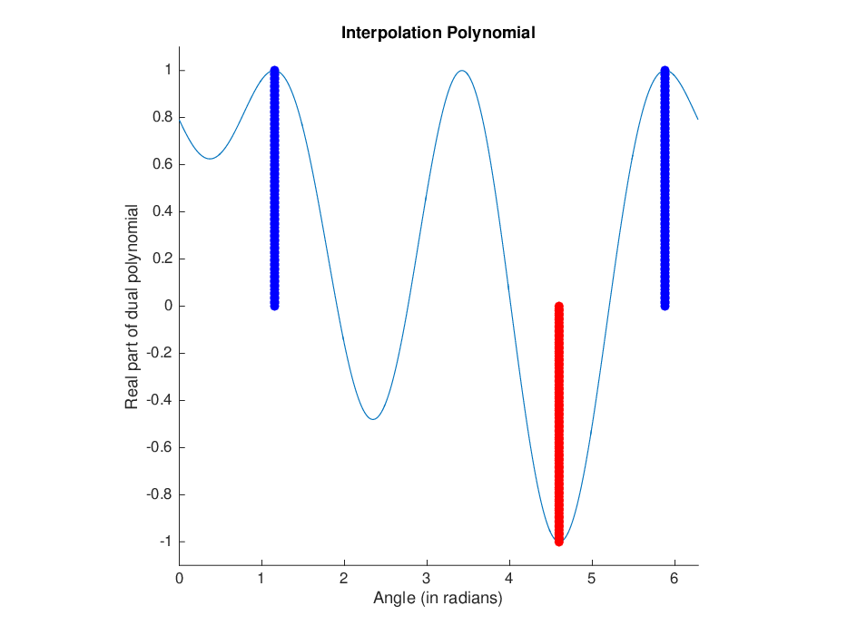
at step of the SDP hierarchy (i.e. in (3.25)). The proximity of points on the torus is thus directly related to the proximity of the exponents of the polynomial. It can be seen in the left part of Figure 2 that some of the point on the torus are very close to one another.
Let us secondly evaluate in the blackbox polynomial at the points
| (4.3) |
at step of the SDP hierarchy. The proximity of points on the torus is thus no longer related to the proximity of the exponents of the polynomial. It can be seen in the left part of Figure 3 that the points on the torus are nicely spread out. This is not guaranteed to be the case, but is expected to be true for small values of (since are well separated in for small ). In order to recover the blackbox polynomial once a candidate atomic measure is computed, we form a table of the integers modulo . For each atom, we consider its argument and find the closest value in the table, yielding an integer , i.e. the power of the monomial associated to the atom. The coefficient of the monomial is given by the weight of the atom.
We now provide numerical experiments. Table 1 and Table 2 show the optimal value and the number of atoms of the optimal measure at each order . Graphical illustrations of the solutions appear in Figure 2 and Figure 3. The dual polynomials in the right hand of the figures illustrate why a higher degree is needed when the points are closer.
| Order | ||
|---|---|---|
| 0 | 2.0000 | 1 |
| 1 | 7.6618 | 2 |
| 2 | 8.1253 | 3 |
| 3 | 8.3655 | 5 |
| 4 | 8.7240 | 7 |
| 5 | 8.9882 | 9 |
| 6 | 9.3433 | 11 |
| 7 | 9.5837 | 13 |
| 8 | 9.7993 | 17 |
| 9 | 9.9436 | 19 |
| 10 | 9.9978 | 20 |
| 11 | 10.0000 | 3 |
| Order | ||
|---|---|---|
| 0 | 2.0000 | 1 |
| 1 | 8.7759 | 2 |
| 2 | 9.2803 | 3 |
| 3 | 10.0000 | 3 |
Remark 1
Before we move on to other examples, we note that naive LP with evaluations at random points on the real line requires about 50 evaluations on this example, compared with the 4 evaluations with super-resolution using multiple loops and in fact, the rigorous LP on the torus also requires 4 evaluations.


4.2 Methodology for comparison
Our methodology for comparing the various approaches is as follows.
- 1.
Generation of the examples: We define a random set of ten sparse polynomials with up to ten variables and up to degree ten (first column of Table 3). We believe that polynomials of higher degree are not realistic and are rarely used in numerical computations. For example, for a polynomial of variables and atoms, we generate the exponents of the monomials randomly from and the associated non-zero coefficients are drawns from a uniform distribution in the interval .
- 2.
Results in the noiseless case: We detect the minimum number of evaluations for each approach to recover the blackbox polynomial in the noiseless case and report the results in Table 3. We use evaluations at the points with up to a certain degree . The corresponding number of evaluations and degree are reported in the columns Rigorous LP, super-resolution, and Toeplitz Prony of Table 3. In Advanced T. Prony, evaluations are made at different points. Thus, only the first three columns of Table 3 can be compared in presence of noise.
- 3.
Results in the presence of noise: For each of the ten polynomials in the list of examples, we determine the maximum degree for the evaluations with and , among Rigorous LP, super-resolution, and Toeplitz Prony in Table 3. For example, for the first line of Table 3, that number is which corresponds to evaluations in this univariate problem. As a result, we know that for these evaluations all three approaches return the correct sparse polynomial. We then add uniform noise to those evaluations, i.e.
(4.4) for all and . Next, we run each approach ten times (with new noise every time) and report the average error in Table 4. The error is defined as the relative error in percentage of the output polynomial compared with the blackbox polynomial using the 2 norm of the coefficients, i.e.
(4.5) Note that in Rigorous LP and super-resolution the equalities associated to the evaluations are relaxed to inequalities, a functionality which is not possible in Toeplitz Prony. This allows for more robutness. Precisely, in Rigorous LP, we replace by and , while in super-resolution we use a 2-norm ball of radius (similar to the technique employed in [7]).
̧ Blackbox Rigorous Super Toeplitz Advanced Polynomial LP Resolution Prony T. Prony 2 (1) 3 (2) 3 (2) 3 4 (3) 5 (4) 4 (3) 4 5 (4) 6 (5) 6 (5) 6 19 (3) 31 (4) 10 (2) 6 10 (2) 19 (3) 19 (3) 13 10 (2) 19 (3) 19 (3) 14 7 (1) 28 (2) 28 (2) 9 28 (2) 28 (2) 28 (2) 16 136 (2) 136 (2) 136 (2) 30 N. A. 1595 (2) 1595 (2) 65
| Blackbox | Rigorous | Super | Toeplitz |
| Polynomial | LP | Resolution | Prony |
| 4.18% | 1.58% | 0.61% | |
| 1.94% | 1.81% | 0.85% | |
| 1.47% | 1.40% | 0.69% | |
| 3.23% | 4.84% | 2.26% | |
| 1.13% | 0.87% | 1.29% | |
| 1.23% | 1.08% | 6.28% | |
| 0.79% | 0.70% | 0.50% | |
| 2.19% | 1.03% | 1.39% | |
| 0.94% | 1.15% | 1.04% | |
| N. A. | 0.47% | 0.46% |
The Advanced T. Prony column of Table 3: the first exponents are chosen (where is the number of monomials in the blackbox polynomias) for the monomials indexing the rows and the first exponents with are chosen for indexing the columns of the Toeplitz matrix. Since , the number of evaluations does not include the conjugate of known values of . The number of monomials is unknown but one could use Advanced T. Prony with successively. We only report the result when setting to the number of monomials in the blackbox polynomial. Note that in the other approaches in Table 3, we do not assume that the number of monomials is known. Same goes in the presence of noise.
4.3 Discussion
Disclaimer: In the sequel, we discuss various advantages and drawbacks of the three methods and of course the resulting conclusions should be interpreted with care as they are biased by the examples that we have considered.
In the noiseless case, Rigorous LP generally requires the least number of evaluations compared with super-resolution and Toeplitz Prony as can be seen in Table 3. This is a remarkable situation where the sparse recovery approach (Rigorous LP) is guaranteed to recover the polynomial even if the RIP property does not hold. The classical result on Prony’s method is that the number of evaluations to recover the blackbox polynomial is equal to twice the number of monomials in the blackbox polynomial (in the univariate case). Toeplitz Prony goes further: the number of evaluations is equal to the number of monomials plus one (in the univariate case, as explained in Section 2.3.2). For example, the third example in Table 3 requires 6 evaluations and is composed of 5 monomials.
In terms of certification, in principle, super-resolution has to be applied with enough points ( for , for and more if the separation between the points is small [7]) to guarantee the existence of a dual certificate polynomial. Moreover, in the multivariate case, no bound on the order of the SDP relaxation is known to guarantee that the flat extension property is satisfied (rank conditions (3.26)-(3.27))55 5 In a few cases where (3.26)-(3.27) are not satisfied, we are still able to a recover polynomial using the algorithm in Section 2.3.1.. In contrast, Toeplitz Prony requires evaluations at points with where is at most the number of monomials, in order to recover the decomposition of the sparse polynomial. In practice, the experimentations show that a small number of evaluations is sufficient to compute the decomposition in both methods.
In terms of computational burden, among Rigorous LP, super-resolution, and Toeplitz Prony, the cheapest approach is Toeplitz Prony since it requires only two linear algbebra operations on matrices of size dependent on the number of monomials in the blackbox polynomials. super-resolution entails a heavy computational burden with the semidefinite optimization. Rigorous LP requires the longest setup time because a variable has to be created for each potential monomial in the blackbox polynomial, unlike the two other approaches. In particular, the setup time is too long on a standard laptop for the example with 10 variables (hence N. A. in Table 3 and Table 4). Howevever, after the setup step has been performed, computing the LP is fast and reliable.
Concerning noise, it seems that the three methods perform more and less equally well even with the relatively large noise level that we have selected, namely 0.1 error on the evaluations. This is little bit surprising for the Prony method because it seems to be commonly admitted that Prony is not very robust to noise. This surprising relative robustness may be due to the large threshold allowed in the rank determination of the SVD decomposition. Indeed, if we select a smaller threshold, we observe degradation of the results for Prony (and super resolution which relies on Prony for the extraction step after the optimization step). See table 5 below.
| Blackbox | Super Resolution | Toeplitz Prony | ||||||
| Polynomial | ||||||||
| 1.58% | 1.58% | 1.58% | 1.58% | 0.79% | 0.79% | 0.79% | 0.79% | |
| 1.80% | 1.80% | 1.80% | 1.80% | 0.91% | 1.15% | 1.15% | 1.15% | |
| 1.42% | 1.44% | 1.44% | 1.44% | 0.68% | 0.68% | 0.68% | 0.68% | |
| 4.69% | 17.25% | 12.49% | 25.50% | 5.35% | 137.90% | 165.79% | 226.29% | |
| 0.93% | 2.10% | 42.69% | 47.50% | 1.22% | 60.36% | 53.86% | 42.47% | |
| 1.00% | 17.56% | 43.39% | 67.55% | 8.45% | 89.45% | 45.82% | 33.87% | |
| 0.78% | 0.78% | 72.17% | 62.02% | 0.41% | 96.50% | 77.42% | 83.27% | |
| 1.09% | 18.55% | 86.55% | 83.45% | 3.59% | 66.02% | 39.77% | 55.15% | |
| 0.85% | 24.60% | 105.84% | 140.05% | 1.68% | 130.39% | 86.77% | 79.96% | |
| 0.54% | 0.54% | 136.20% | 146.93% | 6.45% | 251.17% | 119.65% | 257.64% | |
5 Another efficient (a priori heuristic) approach
In sequel we propose still use the super-resolution hierarchy (3.25) but now by restricting the evaluations at points with
| (5.1) |
This is illustrated in Figure 4. This restriction is first inspired by the fact that Hankel Prony descibed in Section 2.3.1 is guaranteed to work using only those evaluations. There is another more general inspiration coming from two mathematical results.

We provide a result valid in full generality for atomic measures (with finitely many atoms) which indeed suggests that in practice it may suffice to make evaluations at (instead of ). The resulting semidefinite programs have Toeplitz matrices of the same dimension but include much less linear moment constraints. With 10 variables, the first order semidefinite program of the hierarchy entails matrix variables of size and only linear equalities (instead of 56)! The second order relaxation entails matrix variables of size and linear equalities (instead of 1,596), and the third relaxation entails matrix variables of size and linear equalities (instead of 21,691), and so on. We first remind the reader of a well-known result.
Proposition 5.1 (Consequence of Stone-Weiestrass)
Let denote a multi-indexed sequence of complex numbers and let denote a compact set. If there exists a complex-valued finite Borel measure supported on such that
| (5.2) |
then is the unique complex-valued finite Borel measure to satisfy (5.2).
Proof
Consider another such measure . Then
| (5.3) |
Thanks to the complex Stone-Weiestrass Theorem,
| (5.4) |
for all function continuous with respect to the sup-norm . Therefore .
In practice, whether it be interpolation or optimization, we are generally interested in atomic measures with finitely many atoms (in short, atomic measures in the sequel). The next result establishes that for such atomic measures we do not have to care about conjugates, which in view of Proposition 5.1, we find somewhat counter-intuitive.
Lemma 1
Let denote a multi-indexed sequence of complex numbers. If there exists an atomic complex-valued measure such that
| (5.5) |
then is the unique atomic measure to satisfy (5.5).
Proof
Let us write the measure as
| (5.6) |
where , and , and .
Consider another atomic measure that satisfies (5.5), of the form
| (5.7) |
where , and , and .
Consider the following truncated Hankel matrix
| (5.8) |
where . Thanks to Lemma 2, its rank is equal to when and it is equal to when . Thus . Moreover, when , Lemma 3 implies that
| (5.9) |
where .
We now reason by contradiction. Assume that one of the atoms of , say , is distinct from the atoms of . Hence are distinct points of . Lemma 2 implies that
| (5.10) |
are linearly independent vectors if . This contradicts equation (5.9). The atoms of and thus coincide. Their weights satisfy
| (5.11) |
Again, thanks to Lemma 2, the vectors are linearly independent if , thus . This terminates the proof.
Numerical experiments:
Below, we replicate the experiments of Section 4.2 (with and without noise) but now we make evaluations in instead of .
̧ Blackbox Rigorous Super Hankel Advanced Polynomial LP Resolution Prony H. Prony 2 (1) 3 (2) 4 (3) 4 4 (3) 5 (4) 6 (5) 6 5 (4) 6 (5) 10 (9) 10 10 (3) 15 (4) 10 (3) 7 10 (3) 15 (4) 21 (5) 15 10 (3) 15 (4) 21 (5) 18 10 (2) 10 (2) 20 (3) 10 20 (3) 20 (3) 20 (3) 16 21 (2) 21 (2) 56 (3) 28 66 (2) 66 (2) 286 (3) 58
| Blackbox | Rigorous | Super | Hankel |
| Polynomial | LP | Resolution | Prony |
| 2.32% | 1.66% | 0.97% | |
| 1.71% | 2.31% | 3.33% | |
| 0.80% | 1.64% | 2.89% | |
| 14.91% | 11.03% | 52.14% | |
| 0.73% | 1.01% | 2.13% | |
| 1.19% | 12.30% | 2.67% | |
| 0.82% | 1.32% | 0.93% | |
| 3.29% | 2.13% | 16.99% | |
| 2.90% | 1.64% | 6.74% | |
| 107.87% (1) | 161.36% (1) | 134.87% (1) | |
| N.A. (2) | 2.12% (2) | 134.69% (2) | |
| N.A. (3) | N.A. (3) | 0.57% (3) |
In Table 6, in the column Advanced H. Prony, the first exponents are chosen for the monomials indexing the rows and columns of the Hankel matrix, where is the number of terms in the blackbox polynomial . As in Section 4.2, for the first three columns of Table 6 and Table 7, we do not assume anything to be known about the blackbox polynomial expect for the number of variables and an upper bound on the degree (i.e. 10).
In the presence of noise, the optimization step of super-resolution (before the second step of extraction) seems to behave as an efficient filter as it indeed reduces the error compared with Hankel Prony in 7 out of the 9 comparable instances of Table 7. However, sometimes, the semidefinite program does not provide a good output. Indeed, in the sixth example, among the ten trials there are two trials where the solver runs into numerical issues, which explains the large error of .
6 Conclusion
We have addressed the sparse polynomial interpolation problem with three different approaches: sparse recovery, super resolution, and Prony’s method. The common denominator of the three approaches is our view of a polynomial as a signed atomic measure where the atoms correspond to monomials and the weights to coefficients. Then, on the one hand we can invoke directly results from (discrete) super-resolution theory à la Candès & Fernandez-Granda [7] to show that the unknown black box polynomial is the unique solution of a certain LP on a measure space and also the unique solution of finite-dimensional linear program. On the other hand, invoking Kunis et al. [28] Prony’s method can also be applied. To the best of our knowledge this unifying view of sparse interpolation is new and makes the numerical comparison of the three methods very natural. In our preliminary numerical experiments :
- •
Prony’s method works well and better than expected in the presence of noise.
- •
Super-resolution acts in two steps: a first optimization step and then an extraction procedure applied to the optimal solution. The latter step is nothing less than Prony’s method. We find that this optimization step sometimes helps significantly in the presence of noise.
- •
LP-sparse recovery also works well but its set-up time is quite limiting.
Acknowledgement
The work of the first two authors was funded by the European Research Council (ERC) under the European Union’s Horizon 2020 research and innovation program (grant agreement 666981 TAMING).
Appendix
Lemma 2
If are distinct points of , then are linearly independent vectors, where .
Proof
Consider some complex numbers such that
| (6.1) |
Given , define the Lagrange interpolation polynomial
| (6.2) |
where is an index such that . It satisfies if and if . The degree of is equal to . Thus we may multiply the equation in (6.1) by to obtain
| (6.3) |
Summing over all yields .
Lemma 3
If are linearly independent, and , then where denotes the range.
Proof
If , then and . Conversly, an element of the span with belongs to the the range of if there exists such that
which is equivalent to each of the next three lines:
| (6.4) |
| (6.5) |
| (6.6) |
Since has rank , its transpose has rank . Thus there exists a desired . Likewise, belongs to the the range of if there exists such that
Since has rank , its conjugate transpose has rank . Thus there exists a desired .
References
- (1) Jean-Marc Azaïs, Yohann de Castro, and Fabrice Gamboa. Spike detection from inaccurate samplings. Applied and Computational Harmonic Analysis, 38(2):177–195, 2015.
- (2) Michael Ben-Or and Prasoon Tiwari. A deterministic algorithm for sparse multivariate polynomial interpolation. In Proceedings of the Twentieth Annual ACM Symposium on Theory of Computing, pages 301–309. ACM, 1988.
- (3) Elwyn R. Berlekamp. Nonbinary BCH decoding. IEEE Transactions on Information Theory, 14(2):242–242, 1968.
- (4) Gregory Beylkin and Lucas Monzón. On approximation of functions by exponential sums. Applied and Computational Harmonic Analysis, 19(1):17–48, 2005.
- (5) Emmanuel J. Candès. The restricted isometry property and its implications for compressed sensing C.R. Acad. Sci. Paris Ser. I, 346: 589–592, 2008.
- (6) Emmanuel J. Candès and Carlos Fernandez-Granda. Super-Resolution from Noisy Data. Journal of Fourier Analysis and Applications, 19(6):1229–1254, 2013.
- (7) Emmanuel J. Candès and Carlos Fernandez-Granda. Towards a Mathematical Theory of Super-resolution. Communications on Pure and Applied Mathematics, 67(6):906–956, 2014.
- (8) Emmanuel J. Candes and Y. Plan. A Probabilistic and RIPless Theory of Compressed Sensing. IEEE Transactions on Information Theory, 57(11):7235–7254, 2011.
- (9) Emmanuel J. Candes and Terence Tao. Near-Optimal Signal Recovery From Random Projections: Universal Encoding Strategies? IEEE Transactions on Information Theory, 52(12):5406–5425, December 2006.
- (10) Emmanuel J. Candès and Terence Tao. Decoding by linear programming. IEEE Trans. Inform. Theory, 51(12): 4203–4215, 2005. 2014.
- (11) Emmanuel J. Candès, Justin Romberg and Terence Tao. Stable signal recovery from incomplete and inaccurate measurements. Communications on Pure and Applied Mathematics, 59(8):1207–1223, 2006.
- (12) Raul E. Curto and Lawrence A. Fialkow. Truncated K-Moment Problems in Several Variables J. Operator Theory, 54 (2005), pp. 189–226.
- (13) Gaspard Riche de Baron de Prony. Essai expérimental et analytique: Sur les lois de la dilatabilité de fluides élastique et sur celles de la force expansive de la vapeur de l’alcool, à différentes températures. J. Ecole Polyt., 1:24–76, 1795.
- (14) Annie Cuyt and Wen-shin Lee. Sparse Interpolation and Rational Approximation. In Douglas Hardin, Doron Lubinsky, and Brian Simanek, editors, Contemporary Mathematics, volume 661, pages 229–242. American Mathematical Society, Providence, Rhode Island, 2016.
- (15) Yohann De Castro, Fabrice Gamboa, Didier Henrion, and Jean-Bernard Lasserre. Exact solutions to super-resolution on semi-algebraic domains in higher dimensions. IEEE Trans. Inform. Theory, 63:621–630, 2017.
- (16) George B. Dantzig and Mukund N. Thapa. Linear Programming 1: Introduction. Springer-Verlag New York Inc., New York, 1997.
- (17) Vincent Duval and Gabriel Peyré. Exact support recovery for sparse spikes deconvolution. Foundations of Computational Mathematics, 15(5):1315–1355, 2015.
- (18) Ya Yu Fan and C. Kamath. A comparison of Compressed Sensing and Sparse Recovery Algorithms Applied to Simulation Data. Stat. Optim. Inform. Computing, 4:194–213, 2016.
- (19) Mark Giesbrecht, George Labahn, and Wen-shin Lee. Symbolic–numeric sparse interpolation of multivariate polynomials. Journal of Symbolic Computation, 44(8):943–959, August 2009.
- (20) Gene Golub and Victor Pereyra. Separable nonlinear least squares: The variable projection method and its applications. Inverse Problems, 19(2):R1–R26, 2003.
- (21) Dima Yu Grigoriev, Marek Karpinski, and Michael F. Singer. Fast parallel algorithms for sparse multivariate polynomial interpolation over finite fields. SIAM Journal on Computing, 19(6):1059–1063, 1990.
- (22) Jouhayna Harmouch, Houssam Khalil, and Bernard Mourrain. Structured low rank decomposition of multivariate Hankel matrices. Linear Algebra and its Applications, April 2017.
- (23) Hitham Hassanieh, Piotr Indyk, Dina Katabi, and Eric Price. Nearly optimal sparse fourier transform. In Proceedings of the Forty-Fourth Annual ACM Symposium on Theory of Computing , STOC ’12, pages 563–578. ACM Press, 2012.
- (24) Cédric Josz and Daniel K. Molzahn. Large Scale Complex Polynomial Optimization. arXiv:1508.02068
- (25) Erich Kaltofen and Yagati N. Lakshman. Improved Sparse Multivariate Polynomial Interpolation Algorithms. In Proceedings of the International Symposium ISSAC’88 on Symbolic and Algebraic Computation, ISSAC ’88, pages 467–474, London, UK, 1989. Springer-Verlag.
- (26) Erich L. Kaltofen, Wen-shin Lee, and Zhengfeng Yang. Fast estimates of Hankel matrix condition numbers and numeric sparse interpolation. pages 130–136. ACM Press, 2011.
- (27) Nikolai N Krasovskii. Theory of Motion Control. Nauka, Moscow, 1968. (in Russian).
- (28) Stefan Kunis, Thomas Peter, Tim Römer, and Ulrich von der Ohe. A multivariate generalization of Prony’s method. Linear Algebra and its Applications, 490:31–47, 2016.
- (29) Monique Laurent and Bernard Mourrain. A generalized flat extension theorem for moment matrices. Archiv der Mathematik, 93(1):87–98, 2009.
- (30) James Massey. Shift-register synthesis and BCH decoding. IEEE transactions on Information Theory, 15(1):122–127, 1969.
- (31) Bernard Mourrain. Polynomial-exponential decomposition from moments, 2016. hal-01367730, arXiv:1609.05720.
- (32) Lucien W. Neustadt. Optimization, a Moment Problem, and Nonlinear Programming. Journal of the Society for Industrial and Applied Mathematics Series A Control, 2(1):33–53, 1964.
- (33) Jiawang Nie. Optimality Conditions and Finite Convergence of Lasserre’s Hierarchy Math. Program. Ser. A, 146(1-2): 97–121, 2014.
- (34) V. Pereyra and G. Scherer, editors. Exponential Data Fitting and Its Applications. Bentham Science Publishers, 2012.
- (35) Daniel Potts and Manfred Tasche. Nonlinear approximation by sums of nonincreasing exponentials. Applicable Analysis, 90(3-4):609–626, 2011.
- (36) Richard Roy and Thomas Kailath. ESPRIT-estimation of signal parameters via rotational invariance techniques. IEEE Transactions on Acoustics, Speech, and Signal Processing, 37(7):984–995, 1989.
- (37) Walter Rudin. Real and Complex Analysis. McGraw-Hill Education, New York, 1986.
- (38) Tomas Sauer. Prony’s method in several variables. Numerische Mathematik, pages 1–28, 2016.
- (39) Peter Stoica and Randolph L. Moses. Spectral Analysis of Signals. Pearson/Prentice Hall, Upper Saddle River, N.J, 2005.
- (40) A. Lee Swindlehurst and Thomas Kailath. A performance analysis of subspace-based methods in the presence of model errors. I. The MUSIC algorithm. IEEE Transactions on signal processing, 40(7):1758–1774, 1992.
- (41) Richard Zippel. Probabilistic Algorithms for Sparse Polynomials. In Proceedings of the International Symposiumon on Symbolic and Algebraic Computation, EUROSAM ’79, pages 216–226, London, UK, 1979. Springer-Verlag.
- (42) Richard Zippel. Interpolating polynomials from their values. Journal of Symbolic Computation, 9(3):375–403, 1990.
- (43) I. S. Iohvidov, Hankel and Toeplitz Matrices and Forms: Algebraic Theory. Birkhäuser Verlag, Boston, 1982.
- (44) Matthew T. Comer, Erich L. Kaltofen, and Clement Pernet. Sparse Polynomial Interpolation and Berlekamp/Massey Algorithms That Correct Outlier Errors in Input Values Proceedings of the 2012 International Symposium on Symbolic and Algebraic Computation, ISSAC ’12, pages 138–145, Grenoble, France. 2012.