Testing Minimal Flavor Violation in Leptoquark Models of the $R_{K^{(*)}}$ Anomaly

The relevant leptoquark models generate, among others, operators of the following form:

$$C_{bs\mu\mu}^{\rm NP}(\overline{s_{L}}\gamma^{\mu}b_{L})(\overline{\mu_{L}}\gamma_{\mu}\mu_{L})+C_{bs\tau\tau}^{\rm NP}(\overline{s_{L}}\gamma^{\mu}b_{L})(\overline{\tau_{L}}\gamma_{\mu}\tau_{L}),$$

(15)

with

$$C_{bs\ell\ell}^{\rm NP}=\frac{\lambda_{\ell b}^{*}\lambda_{\ell s}}{M_{T}^{2}}.$$

(16)

We consider the experimental data, ${\rm BR}(B^{+}\to K^{+}\tau^{+}\tau^{-})<2.25\times 10^{-3}$ [18], and ${\rm BR}(B^{+}\to K^{+}\mu^{+}\mu^{-})=(4.4\pm 0.3)\times 10^{-7}$ [19], which give

$$R_{\tau/\mu}\equiv\frac{{\rm BR}(B^{+}\to K^{+}\tau^{+}\tau^{-})}{{\rm BR}(B^{+}\to K^{+}\mu^{+}\mu^{-})}<5\times 10^{3}.$$

(17)

We now examine various possibilities for the representation of $T$ under $SU(3)_{\ell}^{2}$ and their predictions for $\lambda_{\alpha i}$ and, consequently, for $C_{bs\mu\mu}$ and $C_{bs\tau\tau}$.

• •

  $SU(3)_{\ell}^{2}$-singlet:

$$T(1,1)_{SU(3)_{\ell}^{2}}\ \Longrightarrow\ \lambda=0.$$

(18)

The reason is that no combination of $Y^{E}$’s transforms as $(\bar{3},1)_{SU(3)_{\ell}^{2}}$. Thus this MFV model cannot account for the $R_{K^{(*)}}$ anomaly.

• •

  $SU(3)_{L}$-anti-triplet:

The spurion must transform as $(1+8,1)_{SU(3)_{\ell}^{2}}$ and thus

$$T(\bar{3},1)\ \Longrightarrow\ \lambda\propto(1+Y^{E}Y^{E\dagger}).$$

(19)

Given the smallness of the lepton Yukawa couplings, we expect that the leading contribution is lepton-flavor universal and thus cannot account for the $R_{K^{(*)}}$ anomaly.

It could, however, be that the singlet contribution is negligibly small for some reason, and the octet contribution dominates. In the case of octet-spurion dominance, $\lambda\propto Y^{E}Y^{E\dagger}$, we have

$$\frac{C_{bs\tau\tau}^{\rm NP}}{C_{bs\mu\mu}^{\rm NP}}=\frac{y_{\tau}^{4}}{y_{\mu}^{4}}=8\times 10^{4}.$$

(20)

Taking into account that the ${\cal O}(0.25)$ deviation of $R_{K}$ from unity comes from the interference of the SM and leptoquark amplitudes, we find that Eq. (20) implies $R_{\tau/\mu}\sim 10^{8}$, strongly violating the experimental upper bound of Eq. (17). We conclude that having a leptoquark transform as $(\bar{3},1)$ under $SU(3)_{L}\times SU(3)_{E}$ is excluded.

• •

  $SU(3)_{E}$-anti-triplet:

$$T(1,\bar{3})_{SU(3)_{\ell}^{2}}\ \Longrightarrow\ \lambda\propto Y^{E\dagger}.$$

(21)

For all such models, we have the ratio between the $T$-mediated amplitudes given by

$$\frac{C_{bs\tau\tau}^{\rm NP}}{C_{bs\mu\mu}^{\rm NP}}=\frac{y_{\tau}^{2}}{y_{\mu}^{2}}=2.8\times 10^{2}.$$

(22)

Thus, these models predict

$$R_{\tau/\mu}\sim 1.2\times 10^{3},$$

(23)

a factor of 4 below the present bound.

In the previous subsection, we proved that the only viable lepton flavor representation is $(1,\bar{3})_{SU(3)_{\ell}^{2}}$. In this subsection we use the experimental data on $B\to K^{(*)}\nu\bar{\nu}$ to exclude some of these models.

Experiments put the upper bounds ${\rm BR}(B^{+}\to K^{+}\nu\bar{\nu})<1.6\times 10^{-5}$ [20] and ${\rm BR}(B^{+}\to K^{*+}\nu\bar{\nu})<4.0\times 10^{-5}$ [21]. Thus,

$$R_{\nu/\mu}^{(*)}\equiv\frac{{\rm BR}(B^{+}\to K^{(*)+}\nu\bar{\nu})}{{\rm BR}(B^{+}\to K^{(*)+}\mu^{+}\mu^{-})}\mathrel{\hbox to0.0pt{\lower 4.0pt\hbox{\hskip 1.0pt$\sim$}\hss}\raise 1.0pt\hbox{$<$}}40.$$

(24)

The relevant leptoquark models generate, among others, operators of the following form:

$$C_{bs\mu\mu}(\overline{s_{L}}\gamma^{\mu}b_{L})(\overline{\mu_{L}}\gamma_{\mu}\mu_{L})+C_{bs\nu_{\tau}\nu_{\tau}}(\overline{s_{L}}\gamma^{\mu}b_{L})(\overline{\nu_{\tau}}\gamma_{\mu}\nu_{\tau}).$$

(25)

The SM predicts [22, 23]

$$C_{bs\nu\nu}^{\rm SM}/C_{bs\mu\mu}^{\rm SM}=-1.49.$$

(26)

(Note that $C_{bs\nu\nu}^{\rm SM}$ is the value for a single flavor, and thus the SM prediction is $R_{\nu/\mu}\sim 6.6$.) The $R_{K^{(*)}}$ anomaly requires

$$C_{bs\mu\mu}^{\rm NP}/C_{bs\mu\mu}^{\rm SM}=-0.12.$$

(27)

We now obtain the ratio $C_{bs\nu_{\tau}\nu_{\tau}}^{\rm NP}/C_{bs\mu\mu}^{\rm NP}$ for each of $T$, $U_{3}^{\mu}$ and $U_{1}^{\mu}$, and the resulting prediction for $R_{\nu/\mu}$:

$$R_{\nu/\mu}\sim\frac{2|C_{bs\nu\nu}^{\rm SM}|^{2}+|C_{bs\nu_{\tau}\nu_{\tau}}^{\rm NP}+C_{bs\nu\nu}^{\rm SM}|^{2}}{|C_{bs\mu\mu}^{\rm NP}+C_{bs\mu\mu}^{\rm SM}|^{2}}.$$

(28)

Note that for $R_{\tau/\mu}$ we had to consider only the lepton flavor representation of the leptoquark. In contrast, for $R_{\nu/\mu}$, the result depends also on the Lorentz and $SU(2)\times U(1)$ representation and is thus different among the three models.

• •

  $T(3,3)_{-1/3}$:

  $$\frac{C_{bs\nu_{\tau}\nu_{\tau}}^{T}}{C_{bs\mu\mu}^{T}}=-\frac{y_{\tau}^{2}}{2y_{\mu}^{2}}\ \Longrightarrow\ R_{\nu/\mu}\sim 3.1\times 10^{2}.$$

  (29)

• •

  $U_{3}^{\mu}(3,3)_{+2/3}$:

  $$\frac{C_{bs\nu_{\tau}\nu_{\tau}}^{U_{3}}}{C_{bs\mu\mu}^{U_{3}}}=-\frac{2y_{\tau}^{2}}{y_{\mu}^{2}}\ \Longrightarrow\ R_{\nu/\mu}\sim 5.6\times 10^{3}.$$

  (30)

• •

  $U_{1}^{\mu}(3,1)_{+2/3}$:

  $$\frac{C_{bs\nu_{\tau}\nu_{\tau}}^{U_{1}}}{C_{bs\mu\mu}^{U_{1}}}=0\ \Longrightarrow\ R_{\nu/\mu}\sim 8.5.$$

  (31)

We conclude that, for the $(1,\bar{3})_{SU(3)_{\ell}^{2}}$ representation, the $T$ and $U_{3}^{\mu}$ models are excluded by the upper bound on $R_{\nu/\mu}$. On the other hand, the $U_{1}^{\mu}$ models predict this ratio to be a factor of 4.7 below the present bound (or, equivalently, 1.3 above the SM prediction).

There are four classes of MLFV models for leptoquarks that can a-priori (that is, without imposing MLFV) generate the operator of Eq. (3):

• •

  Models where it does not couple to the leptons. These are the models where the leptoquark transforms as $(1,1)_{SU(3)_{\ell}^{2}}$.

• •

  Models where the couplings are lepton-flavor-universal to a good approximation. This is the case if the leptoquark transforms as $(\bar{3},1)_{SU(3)_{\ell}^{2}}$ and the leading spurion is a lepton flavor singlet.

• •

  Models where the leptoquark couplings are quadratic in the lepton-Yukawa. This is the case if the leptoquark transforms as $(\bar{3},1)_{SU(3)_{\ell}^{2}}$ and the leading spurion is a lepton flavor octet.

• •

  Models where the leptoquark couplings are linear in the lepton-Yukawa. These is the case if the leptoquark transforms as $(1,\bar{3})_{SU(3)_{\ell}^{2}}$.

Only the latter class is good for explaining the $R_{K^{(*)}}$ anomaly (without violating the $R_{\tau/\mu}$ bound). This MFV classification is common to all three viable leptoquark models: $T(3,3)_{-1/3}$, $U_{3}^{\mu}(3,3)_{+2/3}$, and $U_{1}^{\mu}(3,1)_{+2/3}$. However, additional processes put further constraints:

• •

  The upper bounds on ${\rm BR}(B\to K^{(*)}\nu\bar{\nu})$ exclude the MFV-$T$ and MFV-$U_{3}^{\mu}$ models.

• •

  In Appendix A we show that the MFV-$T$ model is excluded also by the upper bound on new physics contribution to $B_{s}-\overline{B_{s}}$ mixing.

We conclude that the only model that is not excluded by the above consideration is the $U_{1}^{\mu}$ model in the $(1,\bar{3})_{SU(3)_{\ell}^{2}}$ representation.

To make further progress, we need to consider the $SU(3)_{q}^{3}$ representation of the leptoquark, which we do in the next section.

Given the couplings in Table 1, we can now translate the $R_{K^{(*)}}$ requirement,

$$C_{bs\mu\mu}=\sum_{i}\frac{\lambda_{\mu\mu ib}^{*}\lambda_{\mu\mu is}}{M_{\mu i}^{2}}\sim\frac{10^{-3}}{{\rm TeV}^{2}},$$

(39)

into a constraint on the model parameters.

• •

  $U_{U}$:

  $$C_{bs\mu\mu}=\frac{|b|^{2}y_{\mu}^{2}y_{t}^{2}V_{tb}V_{ts}^{*}}{M_{\mu t}^{2}}\ \Longrightarrow\ \frac{b}{M_{U}}\sim\frac{263}{{\rm TeV}}.$$

  (40)

• •

  $U_{Q}$:

  $$C_{bs\mu\mu}=\frac{|b|^{2}y_{\mu}^{2}y_{t}^{2}V_{tb}V_{ts}^{*}}{M_{\mu i}^{2}}\left(2{\cal R}e(x_{1/8})+y_{t}^{2}|V_{tb}|^{2}\right).$$

  (41)

  In order that to have destructive interference with the SM amplitude, we need $2{\cal R}e(x_{1/8})+y_{t}^{2}|V_{tb}|^{2}>0$, namely (assuming that $x_{1/8}$ is real)

  $$x_{1/8}>-0.5.$$

  (42)

• •

  $U_{D}$:

  $$C_{bs\mu\mu}=\frac{|b|^{2}y_{\mu}^{2}y_{b}^{2}y_{t}^{2}V_{tb}V_{ts}^{*}}{M_{\mu b}^{2}}\left(x_{1/8}^{*}+y_{t}^{2}|V_{tb}|^{2}\right).$$

  (43)

  In order that to have destructive interference with the SM amplitude, we need $x_{1/8}+y_{t}^{2}|V_{tb}|^{2}>0$, namely

  $$x_{1/8}>-1.$$

  (44)

Within the MFV models that we study, the requirement that the leptoquarks contribute to the Wilson coefficient of the operator of Eq. (3), namely to the $b\to s\mu^{+}\mu^{-}$ decay, implies that they contribute also to $b\bar{b}\to\ell^{+}\ell^{-}$ scattering processes [24]. MFV suggests that the largest contribution will be to the final $\tau^{+}\tau^{-}$ state. This contribution is constrained by the LHC searches for the $\tau^{+}\tau^{-}$ signature.

In Ref. [24], the results of the ATLAS searches [25, 26] have been recast into bounds on vector leptoquarks mass and coupling:

$$C_{bb\tau\tau}^{U}=\frac{|\lambda_{\tau\tau bb}|^{2}}{M_{U}^{2}}\mathrel{\hbox to0.0pt{\lower 4.0pt\hbox{\hskip 1.0pt$\sim$}\hss}\raise 1.0pt\hbox{$<$}}2.6\ (4.0)\ {\rm TeV}^{-2},$$

(45)

where the stronger (weaker) bound applies in case that $M_{U}>2$ TeV ($M_{U}\mathrel{\hbox to0.0pt{\lower 4.0pt\hbox{\hskip 1.0pt$\sim$}\hss}\raise 1.0pt\hbox{$<$}}2$ TeV), which is above (within) the LHC direct reach. The bound for $M_{U}\mathrel{\hbox to0.0pt{\lower 4.0pt\hbox{\hskip 1.0pt$\sim$}\hss}\raise 1.0pt\hbox{$<$}}2$ TeV is not constant and is slightly weaker than 4 TeV^-2 below 1 TeV, which is anyway excluded by the LHC direct searches (see Appendix B). In Fig. 1 we present the excluded region for $M_{U}<2$ TeV, compared to the 1 $\sigma$ allowed region to fit the $R_{K}$ anomaly.

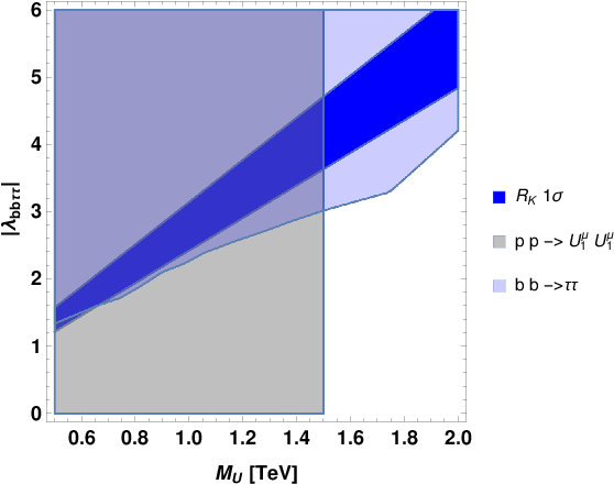
Within our models, we have [see Eq. (64)] $C_{bs\tau\tau}=0.28\ {\rm TeV}^{-2}$. We thus require

$$C_{bb\tau\tau}^{U}/C_{bs\tau\tau}^{U}\mathrel{\hbox to0.0pt{\lower 4.0pt\hbox{\hskip 1.0pt$\sim$}\hss}\raise 1.0pt\hbox{$<$}}9.3(14.3)\ {\rm for}\ M_{U}>(\mathrel{\hbox to0.0pt{\lower 4.0pt\hbox{\hskip 1.0pt$\sim$}\hss}\raise 1.0pt\hbox{$<$}})2\ {\rm TeV}.$$

(46)

The MFV prediction for $C_{bb\tau\tau}$ depends on the quark flavor representation:

• •

  $U_{U}$:

  $$\frac{C_{bb\tau\tau}^{U}}{C_{bs\tau\tau}^{U}}=\frac{V_{tb}}{V_{ts}}\sim 25,$$

  (47)

  which is excluded.

• •

  $U_{Q}$:

  $$\frac{C_{bb\tau\tau}^{U}}{C_{bs\tau\tau}^{U}}=\frac{(x_{1/8}+y_{t}^{2}|V_{tb}|^{2})^{2}}{y_{t}^{2}V_{tb}V_{ts}^{*}(2{\cal R}e(x_{1/8})+y_{t}^{2}|V_{tb}|^{2})}.$$

  (48)

  In the region allowed by $R_{K^{(*)}}$, $x_{1/8}>-0.5$ [see Eq. (42)], the function $(1+x_{1/8})^{2}/(1+2x_{1/8})$ has a minimum value of $1$, and consequently

  $$\frac{C_{bb\tau\tau}^{U}}{C_{bs\tau\tau}^{U}}\mathrel{\hbox to0.0pt{\lower 4.0pt\hbox{\hskip 1.0pt$\sim$}\hss}\raise 1.0pt\hbox{$>$}}\frac{V_{tb}}{V_{ts}}\sim 25,$$

  (49)

  which is excluded.

• •

  $U_{D}$:

  $$\frac{C_{bb\tau\tau}^{U}}{C_{bs\tau\tau}^{U}}=\frac{x_{1/8}+y_{t}^{2}|V_{tb}|^{2}}{y_{t}^{2}V_{tb}V_{ts}^{*}}.$$

  (50)

  Eqs. (44) and (46) imply a narrow allowed window:

  $$-1<x_{1/8}\mathrel{\hbox to0.0pt{\lower 4.0pt\hbox{\hskip 1.0pt$\sim$}\hss}\raise 1.0pt\hbox{$<$}}-0.6(-0.4).$$

  (51)

We conclude that, within the MFV framework, the combined constraints from $R_{K^{(*)}}$ and $b\bar{b}\to\tau^{+}\tau^{-}$ exclude the $U_{U}$ and $U_{Q}$ scenarios, and leave the $U_{D}$ model as the only viable one.

In addition to the measurements of $R_{K^{(*)}}$, there are hints of violation of LFU in $B\to D^{(*)}\tau\nu$ decay. Consider the ratios

$$R_{D^{(*)}}\equiv\frac{\Gamma(B\to D^{(*)}\tau\nu)}{\Gamma(B\to D^{(*)}\ell\nu)},\ \ \ (\ell=e,\mu).$$

(52)

The combination of measurements by BaBar [27, 28], Belle [29, 30, 31, 32] and LHCb [33] reads [34]

$$R_{D}=0.403\pm 0.047,\ \ \ R_{D^{*}}^{\rm SM}=0.310\pm 0.017.\ \ \ \rho=-0.23.$$

(53)

The SM predicts the following values [35, 36, 37, 38]:

$$R_{D}^{\rm SM}=0.300\pm 0.008,\ \ \ R_{D^{*}}^{\rm SM}=0.252\pm 0.003.$$

(54)

Thus, there is a deviation from the SM prediction at $\sim 4\sigma$, with $B\to D^{(*)}\tau\nu$ enhanced with respect to $B\to D^{(*)}\ell\nu$.

Within the MFV framework, the leptoquarks that generate the effective term of Eq. (3), relevant to $b\to s\mu\mu$ decays, generate also the term

$$C_{bc\tau\nu}(\overline{c_{L}}\gamma^{\mu}b_{L})(\overline{\tau_{L}}\gamma_{\mu}\nu_{\tau L}).$$

(55)

In contrast to the $b\to s\mu\mu$ and other processes discussed so far, the $b\to c\tau\nu_{\tau}$ decay is a quark-flavor changing charged current process. We have

$$C_{bc\tau\nu}^{U}=\sum_{i}\frac{\lambda^{*}_{\tau\tau ib}}{M_{\tau i}^{2}}\sum_{j}\lambda_{\tau\tau ij}V_{cj}.$$

(56)

The data require $C^{\rm NP}_{bc\tau\nu}\sim 0.17\ {\rm TeV}^{-2}$. Together with the $R_{K^{(*)}}$ constraint, we need

$$C_{bc\tau\nu}^{\rm NP}/C_{bs\mu\mu}^{\rm NP}\sim-170.$$

(57)

In the $U_{D}$ model, we have the following prediction for $C_{bc\tau\nu}$:

$$C_{bc\tau\nu}^{U}=\frac{|b|^{2}x_{1/8}y_{\tau}^{2}y_{b}^{2}V_{cb}}{M_{\tau b}^{2}}\left(x_{1/8}^{*}+y_{t}^{2}|V_{tb}|^{2}\right).$$

(58)

Thus,

$$\frac{C^{U}_{bc\tau\nu}}{C^{U}_{bs\mu\mu}}=\frac{y_{\tau}^{2}}{y_{\mu}^{2}}\frac{V_{cb}}{V_{ts}^{*}}x_{1/8}\sim+(110-280),$$

(59)

where the range corresponds to $-1<x_{1/8}\mathrel{\hbox to0.0pt{\lower 4.0pt\hbox{\hskip 1.0pt$\sim$}\hss}\raise 1.0pt\hbox{$<$}}-0.4$. The $U_{D}$ model predicts a strong suppression (by at least 10%) of $R_{D^{(*)}}$ from the SM prediction and is thus excluded. In fact, it will remain excluded even if $R_{D^{(*)}}$ turns out to be consistent with the SM prediction (with experimental uncertainties no larger than the present ones) as long as $R_{K^{(*)}}$ is substantially suppressed compared to the SM.

We discuss additional aspects of $R_{D^{(*)}}$ within the MFV framework, independent of $R_{K^{(*)}}$, in Appendix E.

There are three classes of MQFV for leptoquarks that can generate the operator of Eq. (3):

• •

  The $U_{U}$ model in the $(1,3,1)_{SU(3)_{q}^{3}}$ representation. It is excluded by a combination of the $R_{K^{(*)}}$ and $b\bar{b}\to\tau^{+}\tau^{-}$ measurements.

• •

  The $U_{Q}$ model in the $(3,1,1)_{SU(3)_{q}^{3}}$ representation. It is excluded by a combination of the $R_{K^{(*)}}$ and $b\bar{b}\to\tau^{+}\tau^{-}$ measurements.

• •

  The $U_{D}$ model in the $(1,1,3)_{SU(3)_{q}^{3}}$ representation. It is excluded by a combination of the $R_{K^{(*)}}$, $b\bar{b}\to\tau^{+}\tau^{-}$ and $R_{D^{(*)}}$ measurements.

We conclude that all MFV models considered by us are excluded.