跳到论文正文
W Papers独立论文阅读器 arXiv:1708.06129 论文正文 计算阅读时间 · 0%
引用这篇论文根据当前论文元数据生成,正式投稿前建议核对。


License: arXiv.org perpetual non-exclusive license
arXiv:1708.06129v1 [math.DS] 21 Aug 2017

Non-invasive control of the fractional Hegselmann–Krause type model.

Ricardo Almeida1    Agnieszka B. Malinowska2    Tatiana Odzijewicz3 Affiliation: Department of Mathematics, University of Aveiro, Portugal Affiliation: 15-351 Białystok, Poland Affiliation: Warsaw School of Economics Affiliation: 02-554 Warsaw, Poland Affiliation: Center for Research and Development in Mathematics and Applications (CIDMA) Affiliation: Faculty of Computer Science, Bialystok University of Technology Affiliation: Department of Mathematics and Mathematical Economics
Abstract

In this paper, the fractional order Hegselmann–Krause type model with leadership is studied. We seek an optimal control strategy for the system to reach a consensus in such a way that the control mechanism is included in the leader dynamics. Necessary optimality conditions are obtained by the use of a fractional counterpart of Pontryagin Maximum Principle. The effectiveness of the proposed control strategy is illustrated by numerical examples.

Keywords: 
Hegselmann–Krause model, consensus, fractional derivatives, optimal control

1 Introduction

In recent years consensus algorithms for multi-agent systems have been widely discussed in the literature, due to their potential applications in biology [2, 24], physics [25, 27] and engineering areas [10, 14, 19, 21]. The main idea of a consensus algorithm is to drive a team of agents to reach an agreement on a common goal (e.g. positions, velocity, opinion) by interacting with their neighbours. Consensus algorithms are based on nearest-neighbour rules [6, 7, 10, 21], bounded confidence [4, 8, 9, 20] or a virtual leader [3, 23, 28]. The virtual leader is an agent whose motion is independent of all the other agents, and thus is followed by all the other ones.
If a consensus is not achieved, one can apply an optimal control strategy to the system to enforce convergence. For example, in [5] a mathematical model of sparse control was designed in order to attain a consensus. A similar control strategy was proposed in [18] to address a consensus problem in the fractional Cucker–Smale model. In this paper, inspired by [26], we propose a different approach. Namely, we introduce the virtual leader to the system and apply a control function to the leader. This control should steer asymptotically the system to consensus in the most economical way. Therefore, in the cost functional we minimize the transient state deviation and a control effort. Following [26], we call this control strategy non-invasive.

The rest of the paper is organized as follows. In Section 2, we recall necessary concepts and facts on fractional operators and fractional optimal control problems. For a deeper discussion of the fractional calculus and its applications we refer the reader to [1, 11, 12, 13, 15, 16, 17, 22] and references therein. Main results are then stated and proved in Section 3, where we show the existence of optimal controls for the fractional Hegselmann–Krause type model with leadership and the necessary optimality conditions. In Section 4, simulation results are presented in order to demonstrate the validity of the proposed control strategy.

2 Preliminaries

In this section, we give notations and essential facts that will be used in the sequel.

Let [a,b]⊂ℝ[a,b]\subset\mathbb{R} be any bounded interval. For α>0\alpha>0 and f∈L1​([a,b],ℝn)f\in L^{1}([a,b];\mathbb{R}^{n}) we define the left and the right Riemann–Liouville fractional integrals Ia+αI^{\alpha}_{a+} and Ib−αI^{\alpha}_{b-} by

Ia+α​[f]​(t):=1Γ⁡(α)​∫atf⁡(τ)(t−τ)1−α​𝑑τ,t∈[a,b]​a.e.I^{\alpha}_{a+}[f](t):=\frac{1}{\Gamma(\alpha)}\int\limits_{a}^{t}\frac{f(\tau)}{(t-\tau)^{1-\alpha}}\;d\tau,~~t\in[a,b]~a.e.
Ib−α​[f]​(t):=1Γ⁡(α)​∫tbf⁡(τ)(τ−t)1−α​𝑑τ,t∈[a,b]​a.e.I^{\alpha}_{b-}[f](t):=\frac{1}{\Gamma(\alpha)}\int\limits_{t}^{b}\frac{f(\tau)}{(\tau-t)^{1-\alpha}}\;d\tau,~~t\in[a,b]~a.e.

Now, let us define

Ia+α(Lp([a,b];ℝn)):={f:[a,b]→ℝn:∃g∈Lp​([a,b],ℝn)f=Ia+α[g]}I^{\alpha}_{a+}(L^{p}([a,b];\mathbb{R}^{n})):=\left\{f:[a,b]\rightarrow\mathbb{R}^{n}:\exists_{g\in L^{p}([a,b];\mathbb{R}^{n})}f=I^{\alpha}_{a+}[g]\right\}

and

Ib−α(Lp([a,b];ℝn)):={f:[a,b]→ℝn:∃g∈Lp​([a,b],ℝn)f=Ib−α[g]}.I^{\alpha}_{b-}(L^{p}([a,b];\mathbb{R}^{n})):=\left\{f:[a,b]\rightarrow\mathbb{R}^{n}:\exists_{g\in L^{p}([a,b];\mathbb{R}^{n})}f=I^{\alpha}_{b-}[g]\right\}.

For α∈(0,1)\alpha\in(0,1) the left Riemann–Liouville fractional derivatives Da+αD^{\alpha}_{a+} are defined for functions Ia+α​f∈A​C​([a,b],ℝn)I^{\alpha}_{a+}f\in AC([a,b];\mathbb{R}^{n}) by

Da+α​[f]​(t):=dd​t​Ia+α​[f]​(t),t∈[a,b]​a.e.D^{\alpha}_{a+}[f](t):=\frac{d}{dt}I^{\alpha}_{a+}[f](t),~~t\in[a,b]~a.e.

Similarly, for α∈(0,1)\alpha\in(0,1) the right Riemann–Liouville fractional derivatives Db−αD^{\alpha}_{b-} are defined for functions Ib−α​f∈A​C​([a,b],ℝn)I^{\alpha}_{b-}f\in AC([a,b];\mathbb{R}^{n}) by

Db−α​[f]​(t):=dd​t​Ib−α​[f]​(t),t∈[a,b]​a.e.D^{\alpha}_{b-}[f](t):=\frac{d}{dt}I^{\alpha}_{b-}[f](t),~~t\in[a,b]~a.e.

Consider the following fractional optimal control problem:

Da+α​[y]​(t)=g⁡(t,y⁡(t),u⁡(t)),t∈[a,b]​ a.e.,\displaystyle D^{\alpha}_{a+}[y](t)=g(t,y(t),u(t)),~~t\in[a,b]\textnormal{ a.e.}, (1)
Ia+1−α​[y]​(a)=y0,\displaystyle I^{1-\alpha}_{a+}[y](a)=y_{0}, (2)
u⁡(t)∈M⊂ℝm,t∈[a,b],\displaystyle u(t)\in M\subset\mathbb{R}^{m},~~t\in[a,b], (3)
𝒥⁡(y,u)=∫abf⁡(t,y⁡(t),u⁡(t))​𝑑t→min,\displaystyle\mathcal{J}(y,u)=\int\limits_{a}^{b}f(t,y(t),u(t))\;dt\rightarrow\min, (4)

where f:[a,b]×ℝn×M→ℝf:[a,b]\times\mathbb{R}^{n}\times M\rightarrow\mathbb{R}, g:[a,b]×ℝn×M→ℝng:[a,b]\times\mathbb{R}^{n}\times M\rightarrow\mathbb{R}^{n} and α∈(0,1)\alpha\in(0,1).

Definition 1

Suppose that

𝒰M:={u∈L1([a,b];ℝm):u(t)∈M,t∈[a,b]}.\mathcal{U}_{M}:=\left\{u\in L^{1}([a,b];\mathbb{R}^{m}):u(t)\in M,t\in[a,b]\right\}.

A pair (y∗,u∗)∈Ia+α​(Lp)×𝒰M(y_{*},u_{*})\in I^{\alpha}_{a+}(L^{p})\times\mathcal{U}_{M} is said to be locally optimal solution to problem (1)–(4), if y∗y_{*}, corresponding to u∗u_{*}, solves (1)–(2) and there is a neighborhood VV of y∗y_{*} in Ia+α​(Lp)I^{\alpha}_{a+}(L^{p}) such that

𝒥⁡(y∗,u∗)≤𝒥⁡(y,u)\mathcal{J}(y_{*},u_{*})\leq\mathcal{J}(y,u)

for every pair (y,u)∈V×𝒰M(y,u)\in V\times\mathcal{U}_{M} satisfying (1)–(2).

Let ‖⋅‖\left\|\cdot\right\| denote the Euclidean norm. The following theorem is a fractional counterpart of Pontryagin Maximum Principle.

Theorem 2.1

[cf. Theorem 8 and Theorem 9, [13]] Let α∈(0,1)\alpha\in(0,1) and 1≤p<11−α1\leq p<\frac{1}{1-\alpha}. We assume that MM is compact and the following assumptions are satisfied:

  1. 1.

    g∈C1g\in C^{1} with respect to y∈ℝny\in\mathbb{R}^{n} and

    1. (a)

      t↦g⁡(t,y,u)t\mapsto g(t,y,u) is measurable on [a,b][a,b] for all y∈ℝny\in\mathbb{R}^{n}, u∈Mu\in M, u↦g⁡(t,y,u)u\mapsto g(t,y,u) is continuous on MM for t∈[a,b]t\in[a,b] a.e. and all y∈ℝny\in\mathbb{R}^{n};

    2. (b)

      there exists L>0L>0 such that

      ‖g⁡(t,y1,u)−g⁡(t,y2,u)‖≤L⁡‖y1−y2‖\left\|g(t,y_{1},u)-g(t,y_{2},u)\right\|\leq L\left\|y_{1}-y_{2}\right\|

      for t∈[a,b]t\in[a,b] a.e. and all y1,y2∈ℝny_{1},y_{2}\in\mathbb{R}^{n}, u∈Mu\in M;

    3. (c)

      there exist r∈Lp​([a,b],ℝ)r\in L^{p}([a,b];\mathbb{R}) and γ≥0\gamma\geq 0 such that

      ‖g⁡(t,0,u)‖≤r⁡(t)+γ⁡‖u‖\left\|g(t,0,u)\right\|\leq r(t)+\gamma\left\|u\right\|

      for t∈[a,b]t\in[a,b] a.e. and all u∈Mu\in M;

  2. 2.

    t↦f⁡(t,y,u)t\mapsto f(t,y,u) is measurable on [a,b][a,b] for all y∈ℝny\in\mathbb{R}^{n}, u∈Mu\in M and u↦f⁡(t,y,u)u\mapsto f(t,y,u) is continuous on MM for a.e. t∈[a,b]t\in[a,b] and all y∈ℝny\in\mathbb{R}^{n};

  3. 3.

    f∈C1f\in C^{1} with respect to y∈ℝny\in\mathbb{R}^{n} and there exist a¯1∈L1​([a,b],ℝ0+)\bar{a}_{1}\in L^{1}([a,b],\mathbb{R}_{0}^{+}), a¯2∈Lp′​([a,b],ℝ0+)\bar{a}_{2}\in L^{p^{\prime}}([a,b],\mathbb{R}_{0}^{+}) (1p+1p′=1)\left(\frac{1}{p}+\frac{1}{p^{\prime}}=1\right), C¯1,C¯2≥0\bar{C}_{1},\bar{C}_{2}\geq 0 such that

    ‖f⁡(t,y,u)‖≤a¯1​(t)+C¯1​‖y‖p,\displaystyle\left\|f(t,y,u)\right\|\leq\bar{a}_{1}(t)+\bar{C}_{1}\left\|y\right\|^{p}, (5)
    ‖∂∂y​f​(t,y,u)‖≤a¯2​(t)+C¯2​‖y‖p−1,\displaystyle\left\|\frac{\partial}{\partial y}f(t,y,u)\right\|\leq\bar{a}_{2}(t)+\bar{C}_{2}\left\|y\right\|^{p-1}, (6)

    for a.e. t∈[a,b]t\in[a,b] and all y∈ℝny\in\mathbb{R}^{n}, u∈Mu\in M;

  4. 4.

    t↦∂∂y​g​(t,y,u)t\mapsto\displaystyle\frac{\partial}{\partial y}g(t,y,u), t↦∂∂y​f​(t,y,u)t\mapsto\displaystyle\frac{\partial}{\partial y}f(t,y,u) are measurable on [a,b][a,b] for all y∈ℝny\in\mathbb{R}^{n}, u∈Mu\in M;

  5. 5.

    u↦∂∂y​g​(t,y,u)u\mapsto\displaystyle\frac{\partial}{\partial y}g(t,y,u), u↦∂∂y​f​(t,y,u)u\mapsto\displaystyle\frac{\partial}{\partial y}f(t,y,u) are continuous on MM for a.e. t∈[a,b]t\in[a,b] and all y∈ℝny\in\mathbb{R}^{n};

  6. 6.

    for a.e. t∈[a,b]t\in[a,b] and all y∈ℝny\in\mathbb{R}^{n} the set

    Z~:={(f⁡(t,y,u),g⁡(t,y,u))∈ℝn+1,u∈M}\tilde{Z}:=\left\{\left(f(t,y,u),g(t,y,u)\right)\in\mathbb{R}^{n+1},~u\in M\right\} (7)

    is convex.

If the pair

(y∗,u∗)∈(Ia+α​(Lp)+{d(t−a)1−α;d∈ℝn})×𝒰M(y_{*},u_{*})\in\left(I^{\alpha}_{a+}(L^{p})+\left\{\frac{d}{(t-a)^{1-\alpha}};d\in\mathbb{R}^{n}\right\}\right)\times\mathcal{U}_{M}

is a locally optimal solution to problem (1)–(4), then there exists a function λ∈Ib−α​(Lp′)\lambda\in I^{\alpha}_{b-}(L^{p^{\prime}}), such that

Db−α​[λ]​(t)=∂∂y​g​(t,y∗​(t),u∗​(t))T​λ​(t)+∂∂y​f​(t,y∗​(t),u∗​(t))D^{\alpha}_{b-}[\lambda](t)=\frac{\partial}{\partial y}g(t,y_{*}(t),u_{*}(t))^{T}\lambda(t)+\frac{\partial}{\partial y}f(t,y_{*}(t),u_{*}(t)) (8)

for a.e. t∈[a,b]t\in[a,b] and

Ib−1−α​[λ]​(b)=0.I^{1-\alpha}_{b-}[\lambda](b)=0. (9)

Moreover,

f⁡(t,y∗​(t),u∗​(t))+λ⁡(t)​g​(t,y∗​(t),u∗​(t))=minu∈M⁡{f⁡(t,y∗​(t),u)+λ⁡(t)​g​(t,y∗​(t),u)}f(t,y_{*}(t),u_{*}(t))+\lambda(t)g(t,y_{*}(t),u_{*}(t))=\min\limits_{u\in M}\left\{f(t,y_{*}(t),u)+\lambda(t)g(t,y_{*}(t),u)\right\} (10)

for a.e. t∈[a,b]t\in[a,b].

Let g⁡(t,y,u)=A⁡(t)​y​(t)+B⁡(t)​u​(t)g(t,y,u)=A(t)y(t)+B(t)u(t), where A:[a,b]→ℝn×nA:[a,b]\rightarrow\mathbb{R}^{n\times n}, B:[a,b]→ℝn×mB:[a,b]\rightarrow\mathbb{R}^{n\times m}. Then the following theorem, proved in [12], ensures the existence of an optimal solution to problem (1)–(4).

Theorem 2.2

[cf. Theorem 19, [12]] Suppose that 1<p<11−α1<p<\frac{1}{1-\alpha} and

  1. 1.

    MM is convex and compact;

  2. 2.

    t↦f⁡(t,y,u)t\mapsto f(t,y,u) is measurable on [a,b][a,b] for all y∈ℝny\in\mathbb{R}^{n} and u∈Mu\in M;

  3. 3.

    (y,u)↦f⁡(t,y,u)(y,u)\mapsto f(t,y,u) is continuous on ℝn×M\mathbb{R}^{n}\times M for a.e. t∈[a,b]t\in[a,b];

  4. 4.

    u↦f⁡(t,y,u)u\mapsto f(t,y,u) is convex on MM for a.e. t∈[a,b]t\in[a,b] and all y∈ℝny\in\mathbb{R}^{n};

  5. 5.

    A,BA,B are essentially bounded on [a,b][a,b];

  6. 6.

    there exists a summable function ψ1:[a,b]→ℝ0+\psi_{1}:[a,b]\rightarrow\mathbb{R}_{0}^{+} and a constant c1≥0c_{1}\geq 0 such that

    f⁡(t,y,u)≥−ψ1​(t)−c1​‖y‖f(t,y,u)\geq-\psi_{1}(t)-c_{1}\left\|y\right\|

    for a.e. t∈[a,b]t\in[a,b] and all y∈ℝny\in\mathbb{R}^{n}, u∈Mu\in M.

Then problem (1)–(4) possesses an optimal solution

(y0,u0)∈(Ia+α​(Lp)+{d(t−a)1−α;d∈ℝn})×𝒰M.(y_{0},u_{0})\in\left(I^{\alpha}_{a+}(L^{p})+\left\{\frac{d}{(t-a)^{1-\alpha}};d\in\mathbb{R}^{n}\right\}\right)\times\mathcal{U}_{M}.

3 Optimal control of the fractional Hegselmann–Krause type model with leadership

In this section we investigate the fractional optimal control problem with the Hegselmann–Krause type dynamics and leadership. The agents’ and the leader’s opinions are denoted by xix_{i}, i=1,…,Ni=1,\ldots,N, N>1N>1, and x0x_{0}, respectively, and are represented by the state of the system 𝐱=(x0,x1,…,xN)∈ℝ(N+1)​d{\bf x}=(x_{0},x_{1},\dots,x_{N})\in\mathbb{R}^{(N+1)d}.

Let α∈(0,1)\alpha\in(0,1) and x:[0,T]→ℝ(N+1)​dx:[0,T]\rightarrow\mathbb{R}^{(N+1)d}. The control is an integrable function t↦u⁡(t)∈ℝdt\mapsto u(t)\in\mathbb{R}^{d} such that

u⁡(t)∈M:={u⁡(t)∈ℝd:‖u‖l2d≤K},u(t)\in M:=\left\{u(t)\in\mathbb{R}^{d}:\left\|u\right\|_{l_{2}^{d}}\leq K\right\},

where ‖⋅‖l2d\left\|\cdot\right\|_{l_{2}^{d}} denotes the Euclidean norm in ℝd\mathbb{R}^{d}. Consider the problem of finding trajectory solution to the system

{D0+α​[x0]​(t)=u⁡(t),D0+α​[xi]​(t)=∑j=1Nai​j​(xj​(t)−xi​(t))+ci​(x0​(t)−xi​(t)),\begin{cases}D^{\alpha}_{0+}[x_{0}](t)=u(t),\\ D^{\alpha}_{0+}[x_{i}](t)=\sum\limits_{j=1}^{N}a_{ij}(x_{j}(t)-x_{i}(t))+c_{i}(x_{0}(t)-x_{i}(t)),\end{cases} (11)

i=1,…,Ni=1,\dots,N, initialized at I0+1−α​[xj]​(0)=xj​0∈ℝdI^{1-\alpha}_{0+}[x_{j}](0)=x_{j0}\in\mathbb{R}^{d}, j=0,1,…,Nj=0,1,\dots,N. In system (11), the term ∑j=1Nai​j​(xj​(t)−xi​(t))\sum\limits_{j=1}^{N}a_{ij}(x_{j}(t)-x_{i}(t)) comes from the classical Hegselmann–Krause model. The weights ai​j≥0a_{ij}\geq 0 quantify the way that the agents influence each other. The second term ci​(x0​(t)−xi​(t))c_{i}(x_{0}(t)-x_{i}(t)) describes the influence of the leader on the iith agent at the time tt. In the case when the leader state is available to agent ii the value of cic_{i} is positive, otherwise ci=0c_{i}=0. System (11) can be written in the matrix form as follows:

D0+α​[x]​(t)=A​x​(t)+B​u​(t),D^{\alpha}_{0+}[x](t)=Ax(t)+Bu(t),

with x=(x0,x1,…,xN)Tx=(x_{0},x_{1},\ldots,x_{N})^{T}, u=(u0,…,…,0)Tu=(u_{0},\ldots,\ldots,0)^{T},

A=[0d0d⋯0dc1​Ids1​Id⋯a1​N​Id⋯⋯⋱⋯cN​IdaN​1​Id⋯sN​Id],B=[1d0d⋯0d],A=\left[\begin{array}[]{cccc}0_{d}&0_{d}&\cdots&0_{d}\\ \vskip 6.0pt plus 2.0pt minus 2.0pt\cr c_{1}I_{d}&s_{1}I_{d}&\cdots&a_{1N}I_{d}\\ \vskip 6.0pt plus 2.0pt minus 2.0pt\cr\cdots&\cdots&\ddots&\cdots\\ \vskip 6.0pt plus 2.0pt minus 2.0pt\cr c_{N}I_{d}&a_{N1}I_{d}&\cdots&s_{N}I_{d}\end{array}\right],\,\quad B=\left[\begin{array}[]{c}1_{d}\\ \vskip 6.0pt plus 2.0pt minus 2.0pt\cr 0_{d}\\ \vskip 6.0pt plus 2.0pt minus 2.0pt\cr\cdots\\ \vskip 6.0pt plus 2.0pt minus 2.0pt\cr 0_{d}\end{array}\right]\,,

where si=−(∑j≠iai​j+ci)s_{i}=-\bigl(\sum_{j\neq i}a_{ij}+c_{i}\bigr), i=1,…,Ni=1,...,N, IdI_{d} is the identity and 0d0_{d} is the null matrix.

A solution to (11) has to minimize the following cost functional

∫0T[12​N2​∑i,j=1N‖xi​(t)−xj​(t)‖l2d2+12​∑i=1N‖x0​(t)−xi​(t)‖l2d2+ν2​‖u‖l2d2]​𝑑t,\int\limits_{0}^{T}\Biggl[\frac{1}{2N^{2}}\sum\limits_{i,j=1}^{N}\left\|x_{i}(t)-x_{j}(t)\right\|_{l_{2}^{d}}^{2}+\frac{1}{2}\sum\limits_{i=1}^{N}\left\|x_{0}(t)-x_{i}(t)\right\|_{l_{2}^{d}}^{2}+\frac{\nu}{2}\left\|u\right\|_{l_{2}^{d}}^{2}\Biggr]\;dt, (12)

where ν>0\nu>0 is a weight constant.

3.1 Existence of solutions

In this part of the text we discuss the question of existence of solutions to optimal control problem (11)–(12).

Theorem 3.1

If 1<p<11−α1<p<\frac{1}{1-\alpha}, then the Hegselmann–Krause fractional optimal control problem (11)–(12) has an optimal solution (x∗,u∗)(x_{*},u_{*}) in the set

(I0+α​(Lp​([0,T],(ℝd)N+1)+{ct1−α;c∈(ℝd)N+1})×𝒰MCLOSE,\left(I^{\alpha}_{0+}\left(L^{p}([0,T];(\mathbb{R}^{d})^{N+1}\right)+\left\{\displaystyle\frac{c}{t^{1-\alpha}};c\in(\mathbb{R}^{d})^{N+1}\right\}\right)\times\mathcal{U}_{M},

where

𝒰M={u∈L1([0,T];ℝd):u(t)∈M,t∈[0,T]}.\mathcal{U}_{M}=\left\{u\in L^{1}\left([0,T];\mathbb{R}^{d}\right):u(t)\in M,~t\in[0,T]\right\}.
Proof

In order to obtain the desired result, it is enough to show that assumptions of Theorem 2.2 are satisfied. First, let us note that set MM is compact (as it is closed and bounded) and let us define maps g:[0,T]×(ℝd)N+1×M→(ℝd)N+1g:[0,T]\times(\mathbb{R}^{d})^{N+1}\times M\rightarrow(\mathbb{R}^{d})^{N+1},

g⁡(t,x⁡(t),u⁡(t)):=[u⁡(t)∑j=1Nai​j​(xj​(t)−xi​(t))+ci​(x0​(t)−xi​(t))]i=1,…,Ng(t,x(t),u(t)):=\left[\begin{array}[]{l}u(t)\\ \sum\limits_{j=1}^{N}a_{ij}(x_{j}(t)-x_{i}(t))+c_{i}(x_{0}(t)-x_{i}(t))\end{array}\right]_{i=1,\dots,N} (13)

and f:[0,T]×(ℝd)N+1×M→ℝf:[0,T]\times(\mathbb{R}^{d})^{N+1}\times M\rightarrow\mathbb{R},

f⁡(t,x⁡(t),u⁡(t)):=12​N2​∑i,j=1N‖xi​(t)−xj​(t)‖l2d2+12​∑i=1N‖x0​(t)−xi​(t)‖l2d2+ν2​‖u‖l2d2.f(t,x(t),u(t)):=\frac{1}{2N^{2}}\sum\limits_{i,j=1}^{N}\left\|x_{i}(t)-x_{j}(t)\right\|_{l_{2}^{d}}^{2}+\frac{1}{2}\sum\limits_{i=1}^{N}\left\|x_{0}(t)-x_{i}(t)\right\|_{l_{2}^{d}}^{2}+\frac{\nu}{2}\left\|u\right\|_{l_{2}^{d}}^{2}. (14)

It is easy to see that function ff is measurable w.r.t. tt, continuous w.r.t. (x,u)(x,u) and convex w.r.t. uu. Moreover, because AA and BB are matrices with constant coefficients, they are essentially bounded on [0,T][0,T]. Finally, let us note that

f⁡(t,x,u)=12​N2​∑i,j=1N‖xi​(t)−xj​(t)‖l2d2+12​∑i=1N‖x0​(t)−xi​(t)‖l2d2+ν2​‖u‖l2d2≥ν2​‖u‖l2d2,f(t,x,u)=\frac{1}{2N^{2}}\sum\limits_{i,j=1}^{N}\left\|x_{i}(t)-x_{j}(t)\right\|_{l_{2}^{d}}^{2}+\frac{1}{2}\sum\limits_{i=1}^{N}\left\|x_{0}(t)-x_{i}(t)\right\|_{l_{2}^{d}}^{2}+\frac{\nu}{2}\left\|u\right\|_{l_{2}^{d}}^{2}\geq\frac{\nu}{2}\left\|u\right\|_{l_{2}^{d}}^{2},

so choosing ψ1​(t)=−ν2​‖u‖l2d2\psi_{1}(t)=-\frac{\nu}{2}\left\|u\right\|_{l_{2}^{d}}^{2} and c1=0c_{1}=0, we see that the last assumption of Theorem 2.2 is satisfied.

3.2 Necessary optimality conditions

In this section, in order to prove necessary optimality conditions for problem (11)–(12), we show that assumptions of Theorem 2.1 are fulfilled. Let functions ff and gg be defined in the same way as in the proof of Theorem 3.1. First, let us note that in [13] the author showed that under certain assumptions fractional optimal control problem (1)–(4) satisfies the Smooth Convex Extremum Principle (SCEP) (see, e.g., Theorem 3 of [13]) and as a consequence he obtained the Fractional Pontryagin Maximum Principle (Theorem 2.1, see Theorems 8 and 9 of [13]). Among other things, it was shown that if for a.e. t∈[a,b]t\in[a,b] and all y∈ℝny\in\mathbb{R}^{n} the set Z~\tilde{Z} (defined by (7)) is convex, then the convexity assumption in SCEP is satisfied. In the case of problem (11)–(12) we have that for all u1,u2∈𝒰Mu_{1},u_{2}\in\mathcal{U}_{M}, x∈I0+α​(L2​([0,T],(ℝd)N+1))+{ct1−α;c∈(ℝd)N+1}x\in I^{\alpha}_{0+}\left(L^{2}([0,T];(\mathbb{R}^{d})^{N+1})\right)+\left\{\displaystyle\frac{c}{t^{1-\alpha}};c\in(\mathbb{R}^{d})^{N+1}\right\} and θ∈[0,1]\theta\in[0,1] the following hold:

θ​f​(t,x,u1)+(1−θ)​f​(t,x,u2)≥f⁡(t,x,θ​u1+(1−θ)​u2),\theta f(t,x,u_{1})+(1-\theta)f(t,x,u_{2})\geq f(t,x,\theta u_{1}+(1-\theta)u_{2}),
θ​g​(t,x,u1)+(1−θ)​g​(t,x,u2)=g⁡(t,x,θ​u1+(1−θ)​u2)\theta g(t,x,u_{1})+(1-\theta)g(t,x,u_{2})=g(t,x,\theta u_{1}+(1-\theta)u_{2})

with θ​u1+(1−θ)​u2∈𝒰M\theta u_{1}+(1-\theta)u_{2}\in\mathcal{U}_{M}, by convexity of MM. Therefore, the convexity assumption in SCEP is fulfilled. One can easily check that ff, gg are continuously differentiable with respect to x∈(ℝd)N+1x\in(\mathbb{R}^{d})^{N+1} for a.a. t∈[0,T]t\in[0,T] and all u∈ℝdu\in\mathbb{R}^{d} and that t↦g⁡(t,x⁡(t),u⁡(t))t\mapsto g(t,x(t),u(t)), t↦f⁡(t,x⁡(t),u⁡(t))t\mapsto f(t,x(t),u(t)) are measurable on [0,T], also u↦f⁡(t,x⁡(t),u⁡(t))u\mapsto f(t,x(t),u(t)) is continuous on MM. Moreover, x↦g⁡(t,x,u)x\mapsto g(t,x,u) is Lipschitz, u↦g⁡(t,x,u)u\mapsto g(t,x,u) is continuous and

‖g⁡(t,0,u)‖l1N+1−l2d=‖u‖l1N+1−l2d.\left\|g(t,0,u)\right\|_{l_{1}^{N+1}-l_{2}^{d}}=\left\|u\right\|_{l_{1}^{N+1}-l_{2}^{d}}.

Choosing r⁡(t)=0r(t)=0 and γ=1\gamma=1 we conclude that assumption 1 of Theorem 2.1 is satisfied. Note that

∂f∂x=[N​x0−∑i=1Nxi2N​(x1−1N​∑j=1Nxj)+(x1−x0)⋮2N​(xN−1N​∑j=1Nxj)+(xN−x0)]\frac{\partial f}{\partial x}=\left[\begin{array}[]{c}Nx_{0}-\sum\limits_{i=1}^{N}x_{i}\\ \frac{2}{N}(x_{1}-\frac{1}{N}\sum\limits_{j=1}^{N}x_{j})+(x_{1}-x_{0})\\ \vdots\\ \frac{2}{N}(x_{N}-\frac{1}{N}\sum\limits_{j=1}^{N}x_{j})+(x_{N}-x_{0})\end{array}\right] (15)

and system (11) is linear. Therefore, t↦∂f∂x​(t,x,u)t\mapsto\frac{\partial f}{\partial x}(t,x,u), t↦∂g∂x​(t,x,u)t\mapsto\frac{\partial g}{\partial x}(t,x,u) are measurable on [0,T][0,T] and u↦∂f∂x​(t,x,u)u\mapsto\frac{\partial f}{\partial x}(t,x,u), u↦∂g∂x​(t,x,u)u\mapsto\frac{\partial g}{\partial x}(t,x,u) are continuous on MM. Finally, let us check assumption 3 of Theorem 2.1. Observe that

|f⁡(t,x,u)|≤12​N2​∑i,j=1N(‖xi‖l2d2+2​‖xi‖l2d​‖xj‖l2d+‖xj‖l2d2)+12∑i=1N(‖x0‖l2d2+2‖x0‖l2d‖xi‖l2d+‖xi‖l2d2)+ν2‖u‖l2d2=(1N+12)​∑i=1N‖xi‖l2d2+(1N2​∑i=1N‖xi‖l2d+‖x0‖l2d)​∑i=1N‖xi‖l2d+N2​‖x0‖l2d2+ν2​‖u‖l2d2≤∑i=0N‖xi‖l2d2+(∑i=0N‖xi‖l2d)​(∑i=1N‖xi‖l2d)+ν2​‖u‖l2d2≤∑i=1N‖xi‖l2d2+(∑i=0N‖xi‖l2d)2+ν2​‖u‖l2d2≤ν2​‖u‖l2d2+2​‖x‖l1N+1−l2d2,|f(t,x,u)|\leq\frac{1}{2N^{2}}\sum\limits_{i,j=1}^{N}\left(\left\|x_{i}\right\|_{l_{2}^{d}}^{2}+2\left\|x_{i}\right\|_{l_{2}^{d}}\left\|x_{j}\right\|_{l_{2}^{d}}+\left\|x_{j}\right\|_{l_{2}^{d}}^{2}\right)\\ +\frac{1}{2}\sum\limits_{i=1}^{N}\left(\left\|x_{0}\right\|_{l_{2}^{d}}^{2}+2\left\|x_{0}\right\|_{l_{2}^{d}}\left\|x_{i}\right\|_{l_{2}^{d}}+\left\|x_{i}\right\|_{l_{2}^{d}}^{2}\right)+\frac{\nu}{2}\left\|u\right\|_{l_{2}^{d}}^{2}\\ =\left(\frac{1}{N}+\frac{1}{2}\right)\sum\limits_{i=1}^{N}\left\|x_{i}\right\|_{l_{2}^{d}}^{2}+\left(\frac{1}{N^{2}}\sum\limits_{i=1}^{N}\left\|x_{i}\right\|_{l_{2}^{d}}+\left\|x_{0}\right\|_{l_{2}^{d}}\right)\sum\limits_{i=1}^{N}\left\|x_{i}\right\|_{l_{2}^{d}}\\ +\frac{N}{2}\left\|x_{0}\right\|_{l_{2}^{d}}^{2}+\frac{\nu}{2}\left\|u\right\|_{l_{2}^{d}}^{2}\leq\sum\limits_{i=0}^{N}\left\|x_{i}\right\|_{l_{2}^{d}}^{2}+\left(\sum\limits_{i=0}^{N}\left\|x_{i}\right\|_{l_{2}^{d}}\right)\left(\sum\limits_{i=1}^{N}\left\|x_{i}\right\|_{l_{2}^{d}}\right)+\frac{\nu}{2}\left\|u\right\|_{l_{2}^{d}}^{2}\\ \leq\sum\limits_{i=1}^{N}\left\|x_{i}\right\|_{l_{2}^{d}}^{2}+\left(\sum\limits_{i=0}^{N}\left\|x_{i}\right\|_{l_{2}^{d}}\right)^{2}+\frac{\nu}{2}\left\|u\right\|_{l_{2}^{d}}^{2}\leq\frac{\nu}{2}\left\|u\right\|_{l_{2}^{d}}^{2}+2\left\|x\right\|_{l_{1}^{N+1}-l_{2}^{d}}^{2},

and

‖∂f∂x​(t,x,u)‖l1N+1−l2d=‖N​x0−∑i=1Nxi‖l2d+∑i=1N‖2N​(xi−1N​∑j=1Nxj)+(xi−x0)‖l2d≤N​‖x0‖l2d+∑i=1N‖xi‖l2d+(2N+1)​∑i=1N‖xi‖l2d+2N2​∑i=1N‖∑j=1Nxj‖l2d+∑i=1N‖x0‖l2d≤(2+4N)​∑i=0N‖xi‖l2d+2​N​‖x0‖l2d≤2​N​‖x‖l1N+1−l2d.\left\|\frac{\partial f}{\partial x}(t,x,u)\right\|_{l_{1}^{N+1}-l_{2}^{d}}=\|Nx_{0}-\sum\limits_{i=1}^{N}x_{i}\|_{l_{2}^{d}}+\sum\limits_{i=1}^{N}\|\frac{2}{N}(x_{i}-\frac{1}{N}\sum\limits_{j=1}^{N}x_{j})+(x_{i}-x_{0})\|_{l_{2}^{d}}\\ \leq N\|x_{0}\|_{l_{2}^{d}}+\sum\limits_{i=1}^{N}\|x_{i}\|_{l_{2}^{d}}+\left(\frac{2}{N}+1\right)\sum\limits_{i=1}^{N}\|x_{i}\|_{l_{2}^{d}}+\frac{2}{N^{2}}\sum\limits_{i=1}^{N}\|\sum\limits_{j=1}^{N}x_{j}\|_{l_{2}^{d}}+\sum\limits_{i=1}^{N}\|x_{0}\|_{l_{2}^{d}}\\ \leq(2+\frac{4}{N})\sum\limits_{i=0}^{N}\|x_{i}\|_{l_{2}^{d}}+2N\|x_{0}\|_{l_{2}^{d}}\leq 2N\left\|x\right\|_{l_{1}^{N+1}-l_{2}^{d}}.

Choosing a1​(t)=ν2​‖u‖l2d2a_{1}(t)=\frac{\nu}{2}\left\|u\right\|_{l_{2}^{d}}^{2}, a2​(t)=0a_{2}(t)=0 and C1=2C_{1}=2, C2=2​NC_{2}=2N we get desired inequalities. Consequently, all assumptions of Theorem 2.1 are satisfied and we obtain the following theorem.

Theorem 3.2

For α∈(12,1)\alpha\in\left(\frac{1}{2},1\right), if

(x∗,u∗)∈(I0+α​(L2​([0,T],(ℝd)N+1))+{ct1−α;c∈(ℝd)N+1})×𝒰M(x_{*},u_{*})\in\left(I^{\alpha}_{0+}\left(L^{2}([0,T];(\mathbb{R}^{d})^{N+1})\right)+\left\{\displaystyle\frac{c}{t^{1-\alpha}};c\in(\mathbb{R}^{d})^{N+1}\right\}\right)\times\mathcal{U}_{M}

is a locally optimal solution to problem (11)–(12), then there exists a function
λ∈IT−α​(L2​([0,T],(ℝd)N+1))\lambda\in I^{\alpha}_{T-}\left(L^{2}([0,T];(\mathbb{R}^{d})^{N+1})\right) such that

DT−α​[λ]​(t)=AT​λ​(t)+∂∂x​f​(t,x∗​(t),u∗​(t))D^{\alpha}_{T-}[\lambda](t)=A^{T}\lambda(t)+\frac{\partial}{\partial x}f(t,x_{*}(t),u_{*}(t))

for a.e. t∈[0,T]t\in[0,T] and

IT−1−α​[λ]​(T)=0,I^{1-\alpha}_{T-}[\lambda](T)=0,

where ∂f∂x\frac{\partial f}{\partial x} is given by (15). Furthermore,

f⁡(t,x∗​(t),u∗​(t))+λ⁡(t)​g​(t,x∗​(t),u∗​(t))=minu∈M⁡{f⁡(t,x∗​(t),u)+λ⁡(t)​g​(t,x∗​(t),u)}f(t,x_{*}(t),u_{*}(t))+\lambda(t)g(t,x_{*}(t),u_{*}(t))\\ =\min\limits_{u\in M}\left\{f(t,x_{*}(t),u)+\lambda(t)g(t,x_{*}(t),u)\right\} (16)

for a.e. t∈[0,T]t\in[0,T], where ff and gg are given by (14) and (13), respectively.

4 Illustrative examples

In this section, two numerical examples are given to verify the effectiveness of the proposed control strategy.

Example 1

Let us consider the following system

{D0+α​[x0]​(t)=u⁡(t),D0+α​[x1]​(t)=x2​(t)−x1​(t)+x0​(t)−x1​(t),D0+α​[x2]​(t)=x1​(t)−x2​(t),D0+α​[x3]​(t)=x4​(t)−x3​(t)+x0​(t)−x3​(t),D0+α​[x4]​(t)=x3​(t)−x4​(t),I1−α0+[xj](0)=xj​0∈ℝ,j=0,1,2,3,4\begin{cases}D^{\alpha}_{0+}[x_{0}](t)=u(t),\\ D^{\alpha}_{0+}[x_{1}](t)=x_{2}(t)-x_{1}(t)+x_{0}(t)-x_{1}(t),\\ D^{\alpha}_{0+}[x_{2}](t)=x_{1}(t)-x_{2}(t),\\ D^{\alpha}_{0+}[x_{3}](t)=x_{4}(t)-x_{3}(t)+x_{0}(t)-x_{3}(t),\\ D^{\alpha}_{0+}[x_{4}](t)=x_{3}(t)-x_{4}(t),\\ I^{1-\alpha}_{0+}[x_{j}](0)=x_{j0}\in\mathbb{R},~j=0,1,2,3,4\end{cases} (17)

where u⁡(t)∈M:={u⁡(t)∈ℝ:|u⁡(t)|≤1}u(t)\in M:=\left\{u(t)\in\mathbb{R}:|u(t)|\leq 1\right\}. In this case, all agents are connected with each other through the leader x0x_{0} (see Figure 1). Without the presence of the leader, the set {x1,x2}\{x_{1},x_{2}\} does not interact with the set {x3,x4}\{x_{3},x_{4}\} and the dynamic is described by the system

{D0+α​[x1]​(t)=x2​(t)−x1​(t),D0+α​[x2]​(t)=x1​(t)−x2​(t),D0+α​[x3]​(t)=x4​(t)−x3​(t),OPEND0+α​[x4]​(t)=x3​(t)−x4​(t)),I1−α0+[xj](0)=xj​0∈ℝ,j=1,2,3,4.\begin{cases}D^{\alpha}_{0+}[x_{1}](t)=x_{2}(t)-x_{1}(t),\\ D^{\alpha}_{0+}[x_{2}](t)=x_{1}(t)-x_{2}(t),\\ D^{\alpha}_{0+}[x_{3}](t)=x_{4}(t)-x_{3}(t),\\ D^{\alpha}_{0+}[x_{4}](t)=x_{3}(t)-x_{4}(t)),\\ I^{1-\alpha}_{0+}[x_{j}](0)=x_{j0}\in\mathbb{R},~j=1,2,3,4.\end{cases} (18)
Refer to caption
Figure 1: Model with leader and control.

Let us consider the functional

∫0T[132​∑i,j=14(xi​(t)−xj​(t))2+12​∑i=14(x0​(t)−xi​(t))2+u2​(t)]​𝑑t.\int\limits_{0}^{T}\Biggl[\frac{1}{32}\sum\limits_{i,j=1}^{4}(x_{i}(t)-x_{j}(t))^{2}+\frac{1}{2}\sum\limits_{i=1}^{4}(x_{0}(t)-x_{i}(t))^{2}+u^{2}(t)\Biggr]\;dt. (19)

One can easily check that problem of minimizing (19) subject to (17) satisfies assumptions of Theorem 3.2. Let (x∗,u∗)(x_{*},u_{*}) be a solution to problem (17)–(19), then there exists a function λ∈IT−α​(L2​([0,T],ℝ5))\lambda\in I^{\alpha}_{T-}\left(L^{2}([0,T];\mathbb{R}^{5})\right) such that the triple (x∗,u∗,λ)(x_{*},u_{*},\lambda) satisfies the system

DT−α​[λ]​(t)=AT​λ​(t)+[4​x∗0−∑i=14x∗i12​(x∗1−14​∑i=14x∗i)+(x∗1−x∗0)12​(x∗2−14​∑i=14x∗i)+(x∗2−x∗0)12​(x∗3−14​∑i=14x∗i)+(x∗3−x∗0)12​(x∗4−14​∑i=14x∗i)+(x∗4−x∗0)]D^{\alpha}_{T-}[\lambda](t)=A^{T}\lambda(t)+\left[\begin{array}[]{cccc}4x_{*0}-\sum\limits_{i=1}^{4}x_{*i}\\ \frac{1}{2}(x_{*1}-\frac{1}{4}\sum\limits_{i=1}^{4}x_{*i})+(x_{*1}-x_{*0})\\ \frac{1}{2}(x_{*2}-\frac{1}{4}\sum\limits_{i=1}^{4}x_{*i})+(x_{*2}-x_{*0})\\ \frac{1}{2}(x_{*3}-\frac{1}{4}\sum\limits_{i=1}^{4}x_{*i})+(x_{*3}-x_{*0})\\ \frac{1}{2}(x_{*4}-\frac{1}{4}\sum\limits_{i=1}^{4}x_{*i})+(x_{*4}-x_{*0})\end{array}\right] (20)

with

IT−1−α​[λ]​(T)=0.I^{1-\alpha}_{T-}[\lambda](T)=0.

Furthermore,

F⁡(x∗​(t),u∗​(t),λ⁡(t))=minu∈M⁡F⁡(x∗​(t),u,λ⁡(t)),for a.e. ​t∈[0,T],F(x_{*}(t),u_{*}(t),\lambda(t))=\min\limits_{u\in M}F(x_{*}(t),u,\lambda(t)),~\textnormal{for a.e. }t\in[0,T],

where

F⁡(v,u,λ):=132​∑i,j=14(xi−xj)2+12​∑i=14(x0−xi)2+u2+λ0​u+λ1​(x0−2​x1+x2)+λ2​(x1−x2)+λ3​(x0−2​x3+x4)+λ4​(x3−x4).F(v,u,\lambda):=\frac{1}{32}\sum\limits_{i,j=1}^{4}(x_{i}-x_{j})^{2}+\frac{1}{2}\sum\limits_{i=1}^{4}(x_{0}-x_{i})^{2}+u^{2}+\lambda_{0}u\\ +\lambda_{1}(x_{0}-2x_{1}+x_{2})+\lambda_{2}(x_{1}-x_{2})+\lambda_{3}(x_{0}-2x_{3}+x_{4})+\lambda_{4}(x_{3}-x_{4}).

Note that variables xx do not influence on the point, where the minimum of FF is attained, but only on its value. Therefore, an optimal control u∗u_{*} must be such that

u∗2​(t)+λ0​(t)​u​(t)=minu∈M⁡{u2​(t)+λ0​(t)​u​(t)}u_{*}^{2}(t)+\lambda_{0}(t)u(t)=\min\limits_{u\in M}\{u^{2}(t)+\lambda_{0}(t)u(t)\}

for a.e. t∈[0,T]t\in[0,T]. Hence

u∗​(t)={1 if ​λ0​(t)≤−2,−λ0​(t)2 if −2<λ0​(t)<2,−1 if ​λ0​(t)≥2,u_{*}(t)=\begin{cases}1&\text{ if }\lambda_{0}(t)\leq-2,\\ -\frac{\lambda_{0}(t)}{2}&\text{ if }-2<\lambda_{0}(t)<2,\\ -1&\text{ if }\lambda_{0}(t)\geq 2,\end{cases}

where u∗u_{*}, λ\lambda satisfy equations (17), (20), and condition IT−1−α​[λ]​(T)=0I^{1-\alpha}_{T-}[\lambda](T)=0 holds.

Figures below show solutions to systems with and without leader and control, for the fractional orders α=0.6\alpha=0.6 (Figure 2) and α=0.9\alpha=0.9 (Figure 3). We see that, with the presence of the leader and control, the system converges to a consensus faster. The effectiveness of the control strategy is verified.

Refer to caption
Refer to caption
Figure 2: Without (left) and with (right) leader and control, for α=0.6\alpha=0.6.
Refer to caption
Refer to caption
Figure 3: Without (left) and with (right) leader and control, for α=0.9\alpha=0.9.
Example 2

For our second example, consider a system given by three agents and the leader:

{D0+α​[x0]​(t)=u⁡(t),D0+α​[x1]​(t)=x2​(t)−x1​(t),D0+α​[x2]​(t)=x1​(t)−x2​(t),D0+α​[x3]​(t)=x0​(t)−x3​(t),I1−α0+[xj](0)=xj​0∈ℝ,j=0,1,2,3\begin{cases}D^{\alpha}_{0+}[x_{0}](t)=u(t),\\ D^{\alpha}_{0+}[x_{1}](t)=x_{2}(t)-x_{1}(t),\\ D^{\alpha}_{0+}[x_{2}](t)=x_{1}(t)-x_{2}(t),\\ D^{\alpha}_{0+}[x_{3}](t)=x_{0}(t)-x_{3}(t),\\ I^{1-\alpha}_{0+}[x_{j}](0)=x_{j0}\in\mathbb{R},~j=0,1,2,3\end{cases} (21)

where u⁡(t)∈M:={u⁡(t)∈ℝ:|u⁡(t)|≤10}u(t)\in M:=\left\{u(t)\in\mathbb{R}:|u(t)|\leq 10\right\} (Figure 4). In this model, agent x3x_{3} does not interact with agents x1x_{1} and x2x_{2}, independently of the leader presence.
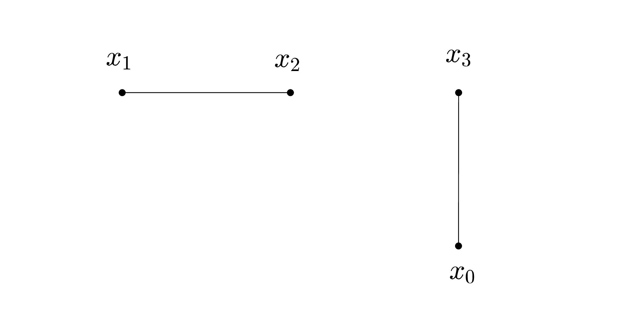
Refer to caption
Figure 4: Model with leader and control.

The objective is to minimize the functional

∫0T[118​∑i,j=13(xi​(t)−xj​(t))2+12​∑i=13(x0​(t)−xi​(t))2+u2​(t)]​𝑑t,\int\limits_{0}^{T}\Biggl[\frac{1}{18}\sum\limits_{i,j=1}^{3}(x_{i}(t)-x_{j}(t))^{2}+\frac{1}{2}\sum\limits_{i=1}^{3}(x_{0}(t)-x_{i}(t))^{2}+u^{2}(t)\Biggr]\;dt,

subject to system (21). Considering the augmented function

F⁡(v,u,λ):=118​∑i,j=13(xi−xj)2+12​∑i=13(x0−xi)2+u2+λ0​u+λ1​(−x1+x2)+λ2​(x1−x2)+λ3​(x0−x3),F(v,u,\lambda):=\frac{1}{18}\sum\limits_{i,j=1}^{3}(x_{i}-x_{j})^{2}+\frac{1}{2}\sum\limits_{i=1}^{3}(x_{0}-x_{i})^{2}+u^{2}+\lambda_{0}u\\ +\lambda_{1}(-x_{1}+x_{2})+\lambda_{2}(x_{1}-x_{2})+\lambda_{3}(x_{0}-x_{3}),

we deduce that the optimal control u∗u_{*} is given by the formula

u∗​(t)={1 if ​λ0​(t)≤−20,−λ0​(t)2 if −20<λ0​(t)<20,−1 if ​λ0​(t)≥20.u_{*}(t)=\begin{cases}1&\text{ if }\lambda_{0}(t)\leq-20,\\ -\frac{\lambda_{0}(t)}{2}&\text{ if }-20<\lambda_{0}(t)<20,\\ -1&\text{ if }\lambda_{0}(t)\geq 20.\end{cases}

In figures below we present plots of agents’ trajectories, with respect to the orders α=0.6\alpha=0.6 (Figure 5) and α=0.9\alpha=0.9 (Figure 6). Again, because of the presence of the leader and control a consensus is reached faster. This demonstrates the effectiveness of the applied control strategy.

Refer to caption
Refer to caption
Figure 5: Without (left) and with (right) leader and control, for α=0.6\alpha=0.6.
Refer to caption
Refer to caption
Figure 6: Without (left) and with (right) leader and control, for α=0.9\alpha=0.9.

Acknowledgements

R. Almeida was supported by Portuguese funds through the CIDMA - Center for Research and Development in Mathematics and Applications, and the Portuguese Foundation for Science and Technology (FCT-Fundação para a Ciência e a Tecnologia), within project UID/MAT/04106/2013; A. B. Malinowska and T. Odzijewicz were supported by Polish founds of National Science Center, granted on the basis of decision DEC-2014/15/B/ST7/05270.

References

  • [1] Almeida, R., Pooseh, S., Torres, D. F. M.: Computational methods in the fractional calculus of variations, Imperial College Press, Singapore (2015)
  • [2] Aoki, I.: A simulation study on the schooling mechanism in fish. Bull. Japan. Soc. Sci. Fish. 48(8), 1081–1088 (1982)
  • [3] Bai, J., Wen, G., Rahmani, A., Chu, X., Yu, Y.: Consensus with a reference state for fractional-order multi-agent systems, Int. J. System Sci., 47(1), 222–234 (2015)
  • [4] Blondel, V. D., Hendrickx, J. M., Tsitsiklis, J. N.: Continuous-time average-preserving opinion dynamics with opinion-dependent communications, SIAM J. Control Optim., 18(8), 5214–5240 (2010)
  • [5] Caponigro, M., Fornasier, M., Piccoli, B., Trelat, E.: Sparse stabilization and optimal control of the Cucker–Smale model. Math. Cont. Related Fields., 3(4), 447–466 (2013)
  • [6] Cucker, F., Smale, S.: Emergent behavior in flocks. IEEE Trans. Automat. Control, 52(5), 852–862 (2007)
  • [7] Girejko, E., Malinowska, A. B., Schmeidel, E., Zdanowicz, M.: The emergence on isolated time scales 21st International Conference on Methods and Models in Automation and Robotics (MMAR), publ. by IEEExplore, 1246–1251 (2016), DOI: 10.1109/MMAR.2016.7575317
  • [8] Girejko, E., Machado, L., Malinowska, A. B., Martins, N.: Krause’s model of opinion dynamics on isolated time scales, Math. Meth. Appl. Sci., 39(18), 5302–5314 (2016)
  • [9] Hegselmann, R., Krause, U.: Opinion dynamics and bounded confidence: models, analysis, and simulation, J. Astif. Soc. Soc. Simul., 5, 1–33 (2002)
  • [10] Jadbabaie, A., Lin, J., Morse,A. S.: Coordination of groups of mobile autonomous agents using nearest neighbor rules. IEEE Trans. Automat. Control, 48(6), 988–1001 (2003)
  • [11] Kaczorek, T.: Selected problems of fractional systems theory. Lecture Notes in Control and Information Sciences, 411, Springer, Berlin (2011)
  • [12] Kamocki, R.: On the existence of optimal solutions to fractional optimal control problems. Appl. Math. Comput., 35, 94–104 (2014)
  • [13] Kamocki, R.: Pontryagin Maximum Principle for fractional ordinary optimal control problems. Math. Meth. Appl. Sci., 37(11), 1668–1686 (2014)
  • [14] Kar, S., Moura Jose, M. F.: Distributed concensus algorithms in sensor networks: quantized data and random link failures, IEEE Trans. Signal Process., 58(3), 1383–1400 (2010)
  • [15] Kilbas, A. A., Srivastava, H. M., Trujillo, J. J.: Theory and Applications of Fractional Differential Equations. North-Holland Mathematics Studies. 204. Elsevier Science B.V., Amsterdam (2006)
  • [16] Malinowska, A. B., Odzijewicz, T., Torres, D. F. M.: Advanced Methods in the Fractional Calculus of Variations, Springer Briefs in Applied Sciences and Technology, Springer International Publishing (2015)
  • [17] Malinowska, A. B., Torres, D. F. M., Introduction to the Fractional Calculus of Variations, Imperial College Press, London & World Sci. Publishing, Singapore (2012)
  • [18] Malinowska, A. B., Odzijewicz, T., Schmeidel, E.: On the existence of optimal controls for the fractional continuous-time Cucker-Smale model, Theory and Applications of Non-integer Order Systems, Eds. A. Babiarz, A. Czornik, J. Klamka, M. Niezabitowski, Lecture Notes in Electrical Engineering 407, 227–240, Springer (2017)
  • [19] Masroor, S., Peng, C., Ali, Z.A.: Event triggered multi-agent consensus of DC motors to regulate speed by LQR scheme, Math. Comput. Appl., 22(1), 1–14 (2017)
  • [20] Mozyrska, D., Wyrwas, M.: Fractional discrete-time of Hegselmann-Krause’s type consensus model with numerical simulations, Neurocomputing, 216, 381–392 (2016)
  • [21] Olfati-Saber, R., Fax, J.A., Murray, R.M.: Consensus and cooperation in networked multi-agent systems. Proceedings of the IEEE, 95(1), 215–233 (2007)
  • [22] Ostalczyk, P.: Discrete Fractional Calculus: Applications in Control and Image Processing, World Scientific Publishing Co. Pte. Ltd., Singapore (2016)
  • [23] Ren, G., Yu, Y., Zhang, S.: Leader-following consensus of fractional nonlinear multiagent systems, Math. Probl. Eng., 2015 (2015), Article ID 919757, 8pp.
  • [24] Reynolds, C. W.: Flocks, herds, and schools: a distributed behavioral model. Comp. Graph., 21(4), 25–34 (1987)
  • [25] Toner, J., Tu, Y.: Flocks, herds, and schools: a quantitative theory of flocking. Phys. Rev. E., 58(4), 4828–4858 (1998)
  • [26] Wongkaew, S., Caponigro, M., Borzí, A.: On the control through leadership of the Hegselmann-Krause opinion formation model. Math. Models Methods Appl. Sci., 3(25), 565–585 (2015)
  • [27] Vicsek, T., Zafeiris, A.: Collective motion. Phys. Rep, 517(3-4), 71–140 (2012)
  • [28] Yu, Z., Jiangn, H., Hu, C.: Leader-following consensus of fractional-order multi-agent systems under fixed topology, Neurocomputing, 149, 613–620 (2015)