Coarsening model on with biased zero-energy flips and an exponential large deviation bound for ASEP
We study the coarsening model (zero-temperature Ising Glauber dynamics) on (for ) with an asymmetric tie-breaking rule. This is a Markov process on the state space of “spin configurations” in which each vertex updates its spin to agree with a majority of its neighbors at the arrival times of a Poisson process. If a vertex has equally many and neighbors, then it updates its spin value to with probability and to with probability . The initial state of this Markov chain is distributed according to a product measure with probability for a spin to be . In this paper, we show that for any given , there exist close enough to 1 such that a.s. every spin has a limit of . This is of particular interest for small values of , for which it is known that if , a.s. all spins have a limit of . For dimension , we also obtain near-exponential convergence rates for sufficiently large, and for general , we obtain stretched exponential rates independent of . Two important ingredients in our proofs are refinements of block arguments of Fontes-Schonmann-Sidoravicius and a novel exponential large deviation bound for the Asymmetric Simple Exclusion Process.
, and
1 Introduction
The coarsening model on with nearest-neighbor edges is defined as follows. Let . Each vertex, , has associated with it an independent Poisson clock of rate 1 and a spin . The state of the system at time is then . Define the energy at to be , where means that is a neighbor of . When the clock at rings, say for the time at time , updates its spin as
where is an independent (of everything else) random variable with
(Formally, we assign an i.i.d. sequence of variables to each site, and use the -th variable at site at the time of the -th update of .) The variables break ties: when , there are equal numbers of and neighbors of , so instead of assuming the majority spin, assumes an independent spin .
The initial state, is assumed to be drawn from the product measure with probability for . Let denote the law of the process with initial configuration , and denote by the joint law of the process and the initial state drawn from the product measure.
1.1 Main result
Observe that for any , the dynamics are attractive with respect to the standard partial ordering of states, where iff for all . This implies that for , if , then one can couple and such that for all , simply by coupling and such that and using the same clocks for both processes. We then define
whenever the set on the right is nonempty. The main purpose of this paper is to ask the following question and to give a partial result.
Question 1.
Is strictly between and for some and ?
We also define
It was shown in [9] that for all , and in [14] it was shown that as . Therefore, one might think that for some small enough and large enough . In other words, if is small and fixed, and we choose large enough so that , changing from (where the system converges to ) to might not be enough to drive the system to . Our main result shows this is false.
Theorem 1.1.
For any fixed and , one has .
Remark 1.2.
A simple consequence of Theorem 1.1 is that the set defining is nonempty. In contrast, it is important to note that the analogue of Theorem 1.1 cannot hold on -regular trees with even values of . (If is odd, there are no ties, and so has no effect.) Indeed, one can show that for small enough, even when , one has for all with positive probability. As a result, the set defining for such is empty. One can prove this by dominating our coarsening model by a bootstrap percolation process with threshold . Therefore if is smaller than the critical probability for bootstrap percolation (which is positive by [4, 7]), some spins in the coarsening model will stay forever.
Theorem 1.1 is a direct consequence of more precise bounds that we derive on fixation times.
Theorem 1.3.
Let .
- 1.
For , there exists and such that
- 2.
For , there exists such that for any real
Theorem 1.3 establishes a near-exponential fixation time in dimension 2 due to an ASEP (Asymmetric Simple Exclusion Process) large deviation estimate, which may be of independent interest, and which we describe below. For dimension , we establish stretched-exponential bounds with dimension-independent exponents by applying erosion time estimates of [6, 11].
To formulate the ASEP large deviation bound, let us first recall the definition of the process. The ASEP is a continuous time Markov chain on particle configurations in (each location can be occupied by at most one particle). For our purposes, it suffices to consider configurations which have a rightmost particle. Each particle has an independent clock with exponential waiting time of mean . When the clock rings, the particle jumps to the right with probability or to the left with probability , provided that the destination is unoccupied (otherwise the jump is forbidden). Let us denote . We consider the ASEP started from the step initial configuration , , and will denote the corresponding probability measure by .
Theorem 1.4.
Let , i.e., the ASEP has drift to the right. Fix any and set . There exists such that for all large enough we have
| (1.1) |
where is an explicit function given in (3.12) below. It is positive and increasing for and behaves as as .
Theorem 1.4 is a one-sided large deviation bound for the integrated ASEP current through zero . Indeed, it is known [13, Theorem 5.12] that the current satisfies the following strong law of large numbers:
(Moreover, the fluctuations of around have order and are governed by the GUE Tracy–Widom distribution [20].) The probability in the left-hand side of (1.1) is essentially the same as
and we obtain a one-sided exponential bound for it (see also Remark 3.6 below for further background on this bound). The proof of Theorem 1.4 is based on asymptotic analysis of the Fredholm determinantal representation for probability distributions in ASEP with the step initial condition and is given in Section 3. Similar analysis was employed in [20] to obtain GUE Tracy–Widom fluctuation behavior for the ASEP, putting this process into the so-called Kardar–Parisi–Zhang universality class.
1.2 Background
We now discuss past results as they relate to question 1. For , when and , almost surely, does not have a limit [2]. Therefore for all . However it is not difficult to show that for and , whenever , one has . Using symmetry, we conclude that for all .
For , it is known [15, Theorem 2] that when , one has
(This is also believed to hold for sufficiently low dimensions [16], while it is thought that fixation may occur when and is sufficiently large [19].) Therefore . By monotonicity of the dynamics in , one furthermore has
In general dimensions , [9] showed that if is close to 1 and , then converges to almost surely. By symmetry between and , then, if is close to 0 and , then converges to almost surely. Thus we deduce that
As a consequence of this and symmetry, one strategy to prove for some would be to show continuity of in .
In dimension , [12] considered the same dynamics as we do here, and studied the asymptotic shape of a large region of ’s surrounded entirely by ’s. In [12], represents an external magnetic field, and and are related by . In the case (), [12] showed that the asymptotic shape of an (initial) by square of ’s satisfies a Law of Large Numbers, in the sense that the region, when rescaled by with time sped up by , follows a deterministic evolution that shrinks to a point in finite time. Moreover, [12] remarks that a similar result holds for all () and all suitable regions of spins. The case , when started from in the first quadrant and elsewhere, corresponds to the TASEP (Totally Asymmetric Simple Exclusion Process) started from the step initial condition, for which [17] computed the almost-sure limiting particle density (shape) when space and time are scaled linearly. These results hint at the near-exponential fixation time in part 1 of Theorem 1.3, but are insufficient to derive it because we require an exponential probability bound on the (linear) speed at which regions shrink.
To give a positive answer to question 1, it would suffice to show that there are some (probably small) values of such that if is arbitrarily close to , then the system will fixate to . The difficulty is that if is small enough, then for long periods of time (depending on ), the system will behave as if , and thus will want to fixate to (due to [9]). Showing that the system will not then “change directions” at a later time and fixate to involves analyzing the configuration at a large , when the variables are highly correlated. Unfortunately, there are few tools available for such analysis.
It is worth noting that other tie-breaking rules have been used in the literature. One option is to set when . This rule is considered, for example, in [3] (for the discrete-time analogue of the coarsening model, usually called the majority vote model) and the process has the same behavior as ours on when an additional edge is placed between each vertex and itself. On this new graph, a vertex has neighbors, so there are no ties, and the additional edge keeps from flipping when ’s original neighbors have an equal number of and spins. Here, one can apply a result of [15], which applies to certain odd-degree graphs to deduce that for each , exists almost surely. However for any , there exist vertices that fixate to , since any side-length two cube of initially spins is stable for all time.
Last, we mention that there exist graphs like finite width slabs (graphs of the form for any ) which have vertices of even degree but for which cannot be strictly less than for . In these graphs, one can construct finite sets of initially spins that are stable for all time.
1.3 Sketch of proof
Due to the above discussion, our main question has to do with the balance between low values of driving the system toward and a bias driving the system toward . Based on the results of [9], the first effect occurs on timescales that are stretched exponential: for small , one has
where is a function of . On the other hand, it is reasonable to believe that the second effect, due to , takes places on exponential time-scales. (At least in case this follows from a comparison to ASEP.)
For large , however, the bias has a strong effect, even when is small, and allows us to prove Theorem 1.1. We now sketch the argument. First consider . In this case, whenever a vertex has or more neighbors with spin, it flips to . We can therefore compare to a Modified Bootstrap Percolation (MBP) process which is defined as follows. Each site begins with a spin, and the distribution of these spins is i.i.d. with probability to be . At each time , each vertex with at least neighbors with spin , all in distinct directions ( for ) flips to . All other spins remain the same — see the definition in Section 2. It is known [18] that for this process, almost surely, each spin eventually fixates to . (It is not sufficient to consider the standard Bootstrap Percolation process, which requires only neighbors with spin to flip to , with no restriction on the directions being distinct. This is due to our identifying -sized blocks with sites in the bootstrap percolation process in the proof of Proposition 2.4, so blocks on opposite sides of a given block have no neighboring vertices in common, and therefore do not aid in the growth of ’s.)
In the original coarsening process with , a spin can flip to if it has at least neighbors with spins, so the coarsening dynamics are not exactly the same as those of the MBP process. However, a comparison with MBP shows that sufficiently large squares have the following property. With high probability (in the size of the square), there is a such that all vertices in have spin at time . Once all the spins in a square become , they will remain forever. We then conclude that for , the coarsening model fixates to . This is stated in Proposition 2.4.
To allow , we choose a large square and pick so that with probability close to 1, at a fixed large time , all spins in are . This places us in a variant of the setting of the FSS argument [9], which is designed to show that the coarsening model will fixate to if the initial condition is sufficiently biased to . In Theorem 4.1, we present a version of the FSS argument in which the initial condition is constant on blocks, and which (in the case ) compares erosion of blocks of spins to the behavior of the ASEP particle system rather than the SEP, as was done in [9]. This comparison allows for a faster fixation rate () for than was given in [9] (). To do this, we give a large deviation bound for ASEP (Theorem 1.4), and this may be of independent interest. In higher dimensions, we apply the results of [6, 11] for the speed of unbiased corner growth to obtain a fixation rate of for any , and this rate also improves on that given in [9]. In Section 5, we combine Theorem 4.1 with Proposition 2.4 to derive Theorem 1.1.
2 Fixation for and
We intend to show that fixation occurs for any initial density when . The argument relies on a result for the Modified Bootstrap Percolation process. Modified Bootstrap Percolation (MBP) is a discrete-time, monotone growth process whose state (or configuration) at step is . For each , we say is occupied at step if , and is vacant otherwise. Given an initial configuration , the deterministic dynamics proceed as follows. A vacant site at step becomes occupied at step if and only if
| (2.1) |
where denotes the standard basis vector, and we let denote the pointwise limit of . In words, if is occupied, it remains occupied forever, and if is vacant, then it becomes occupied if it sees occupied neighbors in all distinct basis directions. The initial configuration is drawn from a product measure on with probability for . For a set , we say that the initial configuration spans if every vertex in eventually becomes occupied, so for every . Define the configuration as
We say that internally spans if spans .
Let . We will make use of the following bound on the probability that MBP internally spans the box , which is Proposition 3.2 in [18].
Lemma 2.1.
Fix and . Then there exists a constant (depending on and ) such that
Remark 2.2.
The definition of the MBP process states that all vertices are updated simultaneously at each step. However, Lemma 2.1 will still hold under other updating rules. The only property necessary for such an updating rule is that at each step, if there is a vertex that is vacant and can be made occupied, then some vertex is made occupied. That is, the order in which vertices are occupied does not matter, as long as no vertex is deliberately ignored. This is the case if, for example, vertices attempt to update their states in continuous time according to independent Poisson processes.
We intend to show that spanning in MBP implies fixation to the all state for the coarsening model when and . A key observation in the case of is that a block of vertices initialized at will remain forever. Indeed, if all (for ) have , then whenever any vertex attempts to flip, it has at least neighbors in the state, and therefore will not flip. The precise statement follows.
Lemma 2.3.
If , and for all , then for all and almost surely.
The next theorem says that in , large boxes tend to fixate to all , regardless of the initial state outside of the box.
Proposition 2.4.
If and , then there exists (depending on and ) such that
When , exists almost surely for each because the number of energy-lowering flips at is almost surely finite (see the remark after Theorem 3 in [15]), and each vertex can undergo at most one energy-neutral flip (to ).
Assume first that is even. We identify , the initial spin configuration, with , an initial MBP configuration. For each , we set if for every and otherwise. Then under , the initial MBP configuration is distributed according to product measure with probability for 1. We claim that if internally spans , then for all . To see why, we argue by induction on the bootstrap time step . So suppose for a fixed that for some and also that for any such that , every vertex in eventually fixates to in the Glauber dynamics. We need to show that every vertex in eventually fixates to in the Glauber dynamics. To start the induction, first note that if , then for each , we have , and by Lemma 2.3, for all .
If , then by the induction hypothesis it follows that every vertex in is eventually in the state. If , then has neighbors, , in different directions such that . By symmetry of the lattice, we may suppose that these neighbors are . We will now use induction on the distance from the vertex to show that every vertex in eventually fixates to in the Glauber dynamics. Fix , and suppose that for every such that (this set is empty if ), the vertex eventually fixates in the state. Consider a vertex with such that ; without loss of generality, suppose (if , then ). For each , the vertex is eventually in the state by the induction hypothesis (on ), and for , the vertex is eventually in the state, since . Therefore, eventually has neighbors frozen in the state, and since it attempts to flip at arbitrarily large times, will eventually fixate to , which concludes the induction on . Therefore, we have that the cube will eventually fixate to , which finishes the induction on .
When is odd, we can apply the even result to each of the boxes for . If all of these boxes have initial configurations that eventually flip to all , then every vertex in the box eventually flips to , so this happens with probability at least . By choosing small enough, this gives the result for all . ∎
Proposition 2.4 will be used later in Section 5 to prove that large boxes can be made to have all spins with high probability at a large time, conditional on the state outside the box, even when is (but very close to 1). Specifically, the reader should see (5.3), which states that for a given and , there exist and such that
This estimate will give us the initial scale at which we will apply Theorem 4.1.
3 Decay of boxes
Let be the time for the configuration in the rectangle, , to reach all , when the dynamics (with -biased tie breaking) is run with an initial configuration of all inside and all outside . It was proved by [9] for dimension , [6] for dimension , and by [11] for dimension that if , then is at most order (up to logarithmic corrections) with high probability. The precise result is as follows.
Theorem 3.1 (Theorem 1.3 in [9], Theorem 3.1 in [6] and Theorem 2.2 in [11]).
Let and . There exists a constant (not depending on ) such that
In fact, [9] proved an exponential probability bound, without the logarithmic correction for . Note that by monotonicity, Theorem 3.1 also holds when . However, in Assumption 1 below, we will require an exponential probability bound (not a polynomial one) on the erosion time of an box. In dimension , we are able to prove that grows linearly with with an exponential probability bound, and in dimensions , we apply Theorem 3.1 in a straightforward manner to obtain a (nearly) cubic bound on .
Theorem 3.2.
Suppose . There is a constant such that the following statements hold.
- 1.
If , then
- 2.
If , then
- 3.
If ,
Remark 3.3.
We suspect that Theorem 3.2 is essentially sharp (with suboptimal constant ) only in case 1 (). In general, we expect the bound in case 1 to hold for all .
Part is a direct consequence of attractiveness and Corollary 3.4 below. Part follows from part by subdividing the three-dimensional box into two-dimensional slices, for . Consider the slowed-down dynamics in which the slices must decay in lexicographic order. That is, the vertices in are not allowed to flip until all of the vertices in are in the state. By attractiveness, the original dynamics dominate these slowed-down dynamics. If is the time for the layer to decay (after layer has decayed) in these slowed-down dynamics, and is the constant from part , which we may assume is larger than without loss of generality, then by part ,
for all . This shows the statement of part 2 with for such . To handle , we simply increase .
We now prove part of the theorem using a restarting argument. Suppose , let be the constant from Theorem 3.1, and for , let . Initialize the configuration to be all inside and all outside at time . Now define a new Markov process as follows. In the time intervals , we let follow the same rules as . At the times , if there exists such that , then set for all . By the obvious coupling, we can construct on the same probability space as such that for all and . Since the all state is absorbing for , we now have
| (3.1) | ||||
which proves part for large if . By choosing large enough, the statement holds for all . ∎
The remainder of this section is devoted to proving the ASEP bound of Theorem 1.4 which, along with attractiveness, implies the following corollary for the coarsening model:
Corollary 3.4.
Consider the two-dimensional coarsening model , , with the initial condition in and elsewhere, and . Fix any . There exists such that for all sufficiently large we have
| (3.2) |
where is given by (3.12) below.
The coarsening model with the quadrant initial configuration described in the hypothesis is the same as the corner growth and decay model with exponential waiting times. The latter model can be coupled to the ASEP with the step initial configuration described before Theorem 1.4, such that
| (3.3) |
see Figure 1. Here under the ASEP the probabilities of right and left jumps are and , respectively. Applying Theorem 1.4 we get the desired estimate (3.2).
∎
Step 1. Pre-limit Fredholm determinant. We first recall a formula from [20, Lemma 4] for with any fixed , as an integral of a Fredholm determinant (recall that ). We need some notation. Let , and denote
This series converges for , and extends analytically to all with poles at . Also set . Fix any and define the kernel
| (3.4) |
where is any number in .11 1 Here and below by a kernel we mean a function of two variables belonging to a certain space. A kernel can be associated with an integral operator acting on functions on this space. For the kernel the variables belong to a circle in the complex plane with center zero and radius .
We will need the Fredholm determinant of the kernel (3.4) of the form . Here is the identity operator, and this Fredholm determinant can be defined by a convergent series
| (3.5) |
That is, one forms determinants of growing order out of the kernel and integrates them over the direct powers of the circle . We refer to [5] for a review of Fredholm determinants.
We will utilize [20, Lemma 4] which states that for the ASEP with the step initial configuration,
| (3.6) |
where is fixed and is the infinite -Pochhammer symbol. Note that in (3.6) the sign in the left-hand side is “” as opposed to [20] because we consider the step initial configuration with particles packed to the left of the origin, and in [20] the particles are packed to the right of it.
Step 2. Critical points. Our goal is to understand the asymptotic behavior of the right-hand side of (3.6) as and with fixed (see Remark 3.6 below for a discussion of what should be expected when ). Let us focus on the integrand in (3.4) and rewrite it as
| (3.7) |
where
| (3.8) |
We have changed the signs to and for later convenience; note that the term always stays bounded as because .
Having all the essential dependence on in the exponent, we employ a standard idea that the asymptotic behavior of the integral in (3.4) and subsequently of the whole Fredholm determinant (3.5) can be derived by the steepest descent method. The critical points of are found from the following equation equivalent to :
When these two roots coincide (and are both equal to ) leading to the GUE Tracy–Widom asymptotics derived in [20]. When the roots are real and distinct. Moreover, they satisfy , . For future convenience we need the following expressions:
Let us define
| (3.9) |
where the expression in the right-hand side is a straightforward computation. Since and which is positive for and behaves as as , we have
| for , as . |
Let us now choose the radii and in (3.4), (3.5) so that the contours for and the ’s pass through our single critical points . Namely, set
| (3.10) |
For the conditions and to hold for (3.10) we need to assume that is not too large, namely,
| (3.11) |
One can readily check that (3.11) implies and .
Because the particles in the ASEP are ordered, the claim of Theorem 1.4 for would also imply the claim for if we truncate the function (3.9). Namely, let us define to be equal to for and to otherwise, that is,
| (3.12) |
Thus defined is weakly increasing in . Therefore, throughout the rest of the proof we can and will assume that is bounded as in (3.11).
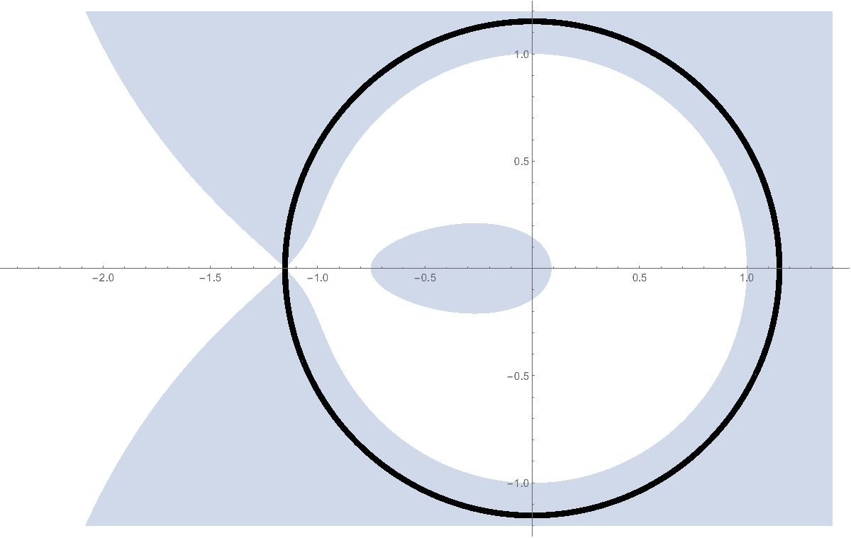
Step 3. Estimates of the real part of . Our next goal is to estimate the real part of the function (3.8) on the circles with the radii (3.10). Namely, let us show that for any :
| 1. For any with , we have . 2. For any with , we have . | (3.13) |
These estimates follow from the straightforward computations:
and
These signs of these derivatives establish (3.13) for in the lower half plane. To obtain these inequalities in the upper half plane one needs to take (and similarly for ) which leads to the opposite signs of the derivatives. See Figure 2 for an illustration.

Step 4. Steepest descent asymptotics of . Fix on a circle of radius . In this step we argue that the main contribution to the asymptotics of as an integral over with comes from a small neighborhood of . All error terms we obtain here and in the next step are uniform in because the contour for is chosen so that is bounded uniformly in .
The -dependence in the integrand in has the form
| (3.14) |
see (3.7). Take a neighborhood of of size . Let us use (3.13) and the estimates of the derivatives in the previous step to bound the absolute value of the integral of (3.14) over the part of the circle outside this neighborhood of . We have
for some (recall that is at most one in absolute value, so we simply estimate this power of by a constant). Inside the -neighborhood of make a change of variables
Here the minus sign in the second term accounts for the direction of the contour in the neighborhood of , and the bound corresponds to the size of the neighborhood. We have
Using (3.7) and the fact that , we can rewrite the integral in (3.4) as
The last integral is a convergent Gaussian integral, and thus we obtain
| (3.15) |
Note that the constant in can be taken independent of on our contours because the quantity is bounded away from zero and infinity.
Step 5. Asymptotics of the Fredholm determinant. We see that (3.15) approximates (viewed as an operator) as by a rank one operator. Therefore, the determinants entering the Fredholm determinant (3.5) are simplified as
where the terms correspond to in (3.15).22 2 Note that here “” in the determinant in the right-hand side is simply the constant entering every matrix element, and not the identity operator. Applying Lemma 3.5 (see below) to the determinant in the right-hand side we see that it is bounded by , where is a bound on . Thus, the whole Fredholm determinant (3.5) can be rewritten as
| (3.16) |
where
| (3.17) |
Both the main term corresponding to in (3.16) and the integrals in the remainder in (3.17) can be estimated using the steepest descent method with the help of (3.13) similarly to Step 4 above.
First, for the single integral in (3.16) we have (in particular, using the fact that the constant in is independent of )
The main contribution to the integral over comes from a small neighborhood of the critical point (recall that ). Making a change of variables leads to a convergent Gaussian integral of ; note that . Therefore, we can continue as
Similarly to Step 4, the constant in can be taken independent of .
In the remainder (3.17) we can similarly bound each integral by (with independent of ). Therefore, the series in (3.17) converges thanks to the factorial in the denominator, and its sum behaves as , which is exponentially negligible compared to the main contribution in (3.16).
Step 6. Completing the proof. Putting all together and using (3.6) we see that
where the remainder (3.17) (the sum of the terms with ) is also incorporated into the term which can be taken independent of . Recall that , so the term stays bounded as . Observe that
as the residue at zero, and that
by residues using the definition of , and by the -binomial theorem. Note that the latter quantity is real and negative as should be. This completes the proof of the large deviation bound of Theorem 1.4. ∎
The following lemma is employed in the above proof of Theorem 1.4:
Lemma 3.5.
Let , where . Then for any and all large enough we have
where .
First, due to the rank one part in (i.e., to the matrix consisting of all ’s), the terms of orders in cancel out. This leaves only two powers of , and , so
Here is a sum of determinants of with one of the rows replaced by the row of ones. Estimating the absolute value of each of these determinants by Hadamard’s inequality and noting that for large the first summand above dominates, we get the desired bound. ∎
Let us conclude with two comments on Theorem 1.4 and its proof given above:
Remark 3.6.
1. A similar approach can be utilized to obtain a one-sided large deviation bound of the form
where is fixed. This is because [20, Lemma 4] provides a pre-limit Fredholm determinantal formula for the probability for any (with a suitably modified kernel ). The function may be explicitly computed using this formula. However, for the analysis of the coarsening model we only need the particular case which is our Theorem 1.4.
2. Our proof of Theorem 1.4 shows that, up to polynomial corrections, the probability
that the ASEP is “too slow” goes to zero at exponential rate. The large deviation probability
at the other tail (that the ASEP is “too fast”) should go to zero at a much faster rate for some other rate function (e.g., see [10] for the case of TASEP). The analysis required to establish this other tail bound for ASEP by the same method as Theorem 1.4 would likely be much more involved. Indeed, in this case the Fredholm determinant would need to go to zero instead of one, and because the critical points have a completely different structure (there are two complex conjugate critical points of with being the same at both of them), the result would require a much more subtle analysis of all terms of the Fredholm expansion (3.5). We do not pursue this superexponential tail here.
4 Application of Fontes-Schonmann-Sidoravicius
In this section we prove a variant of the fixation theorem of Fontes-Schonmann-Sidoravicius (FSS). It states that if the biased coarsening model runs starting from an initial condition in which blocks of size are monochromatic and independent of one another, then if the probability that a block begins in the all state is high enough, then all spins converge to quickly.
We will begin with and split the lattice into disjoint translates of the box . Each box will be filled with spins with probability , and filled with spins otherwise, independently of each other. Then we will run the zero-temperature Glauber dynamics on the original lattice with tie-breaking probability . The corresponding probability measure on the dynamics and initial distribution is denoted .
We will make the following assumption, and its validity will depend on the value of we use.
Assumption 1.
Let be the time for the configuration in the rectangle to reach all , when the dynamics (with -biased tie breaking) is run with an initial configuration of all inside the rectangle and all outside. There exist and such that
| (4.1) |
Note that the measure only depends on , since the initial condition is deterministic. Furthermore, by attractiveness, if (4.1) holds for some and then it holds for with the same . Last, we note here that by Theorem 3.2, the above assumption holds in our coarsening model for in either of the following cases: and , or and any .
The main result is:
Theorem 4.1.
Suppose is such that (4.1) holds for some and constants .
- 1.
If , and is given, there exists with the following property. For any , there exists such that
- 2.
If , and is given, there exists with the following property. For any and
(where the constant is an explicit function of and ), there exists such that
Remark 4.2.
One can argue by attractiveness that item 1 holds for all . Part 1 of the above theorem can be improved, replacing by , or more iterated logarithms. Part 2 can also be improved, replacing by , or more iterated logarithms.
Remark 4.3.
Our proof is a modification of that of Fontes-Schonmann-Sidoravicius (FSS) [9], allowing for a more general erosion rate. Their original arguments used , which comes from a comparison to the Symmetric Exclusion Process (SEP). Morris [14] adapted the arguments of FSS for large dimensions using the SEP estimates, and needed to choose the initial scale (see Theorem 2 in [14]). This is roughly our dependence between and in item 2 above when and is fixed. Our parameters in the case show that one can choose independent of .
The reason why in the case , the proof requires to depend on is seen by attempting to take fixed but (and obtaining a contradiction) in the following bounds. From (4.4), one has (as ). From (4.14), we also find , and so
For , this becomes . On the other hand, the term in (4.3) is a probability bound, so it is only useful if it is bounded by 1: for ,
The second term of this product on the right side is minimized when is the integer part of a constant factor times . For this choice, if we let be fixed and let , we get a contradiction, as .
From here we will copy the arguments of FSS, with modification as appropriate. We will inductively define three sequences ,
and we will set for
Next define cubes of scale , (pictured in Figure 3) as
and larger cubes
with and .
Just as in FSS, we will run a block dynamics, coupled to the original dynamics, so that the evolution of the spins in each box during the time interval will depend only on the configuration at time and the Poisson clocks inside the box . For this we also need the “influence time” associated with the box . Let be the evolution in the box with boundary condition outside this box, started at time from the configuration inside the box. We use in place of or to denote the all initial configurations, and similarly for . Set
We begin the block process at time . With probability , all spins in the box are declared , and with probability they are declared . The status of spins in different boxes is determined independently.
For , use the rules of FSS [9, p. 507]:
-
- Rule 1.
During the time interval we observe the evolution inside the box with boundary conditions. We assign to the spins in the box up to time the values that we see in that evolution.
- Rule 2.
If , then at time , all spins in are declared to be , and persist in this state without change to time .
- Rule 3.
If, following the two rules above, there is any spin in state in at times that are arbitrarily close to , then at time , all the spins in are declared to be . Otherwise, at time all the spins in are declared to be .
- Rule 1.
We next note that the following properties [9, p. 506] hold.
- (A)
The block dynamics favors spins, in the sense that at any site and time where the original dynamics has a spin, the block dynamics also has a spin.
- (B)
In the block dynamics at time , all squares of the -th scale will be monochromatic.
- (C)
For each , the random field that associates to each a random variable which takes the value (respectively ) if at time the block is in state (respectively ) is a -dependent random field.
For the rest of Section 4, all probabilities are evaluated on the space on which we have coupled the original dynamics with the block dynamics.
4.1 Main bounds
Let , denote the probability that at time , the block is in state and note that , since . We will now try to bound the probability of the event
(in steps 1 and 2 below) and of the event
(in step 3 below). Combining these bounds will give us an inequality for in terms of our various parameters (see the top of Section 4.2). After that, we will choose appropriate parameters to ensure that we can prove in Section 4.3 that decreases to zero rapidly.
Step 1. Control of bootstrapping at time . At time , all blocks are monochromatic and we identify each block in the natural way with an element of . For , let
We apply the threshold-two bootstrap percolation rule to the random field in to obtain a collection of well-separated rectangles (no vertex of is at distance from two rectangles), which is minimal among those that contain the renormalized sites with . Precisely, we define a sequence of fields by setting , and for each , we put if has at least two neighbors (in -distance) in with -value equal to . We set otherwise. This sequence is monotone in , so we can set . The collection of vertices with forms a collection of minimal well-separated rectangles. Let for and note that the ’s are also well-separated. By definition, one has .
Estimation of the sizes of the rectangles is similar to that in [9, p. 508-510]. To summarize, one applies the Aizenman-Lebowitz lemma [1, Lemma 1] (restated as [9, Lemma 2.1]), to deduce that if one of the rectangles has one side of length bigger than , then must contain a subrectangle with larger side in which is internally spanned. To bound the probability that there is such an internally spanned subrectangle, we let be any number satisfying
| (4.2) |
(our corresponds to the quantity in the definition of below (4.11) in [9]) and note that the number of rectangles inside with the length of the larger side being in is at most . Next one can also argue that if is an rectangle, then (see [9, Eq. (4.15)])
So if we define
then assuming (4.2), we have
| (4.3) |
Step 2. Erosion of -rectangles. This step follows the corresponding step in [9, p. 510], with the exception that we allow for general in (4.4) below. Since we have just given a bound on the probability of , and we wish to estimate the probability of , we must next upper bound the conditional probability . To do so, we need to consider the system started at time from a configuration in for which can occur and let the system evolve with boundary conditions until time . By attractiveness, an upper bound on the probability that in such a setup, there are spins present at time can be obtained by starting the evolution inside at time with spins at all sites of the rectangles described in step 1 and spins elsewhere in . The spins cannot spread outside of the rectangles , and when a rectangle is taken over by spins, it will never again contain a spin.
If occurs, then each , is contained in a cube of side length bounded by . By attractiveness, the time needed to erode such a cube is therefore stochastically bounded by the time needed to erode a cube with side length . We will then make use of Assumption 4.1 with to conclude that if occurs and
| (4.4) |
then the probability that at time there is any spin inside a fixed is bounded above by
But the number of rectangles satisfies
| (4.5) |
Step 3. Control of the outer influence. This step directly follows the corresponding step in [9, p. 511]. Consider the two evolutions and . We say that at time there is a discrepancy at if there exists some initial such that these evolutions disagree at time at site . Otherwise is an agreement vertex. Note that all vertices in are agreement vertices at time and all vertices outside have discrepancies. The time is defined as the first time a vertex in has a discrepancy.
To estimate the probability that there is a discrepancy in , one first shows that if some vertex in the internal boundary of at time is occupied by a discrepancy, then there exists a chronological path in the time interval which starts at some vertex of the external boundary of and ends at a vertex of the internal boundary of . A chronological path is a self-avoiding path whose vertices are first occupied by discrepancies in order along the path. See [9, p. 511-512] for a proof. Next, one can use the Chernoff bound for Poisson random variables to prove that the probability that any path with vertices is a chronological path during the time period is at most . From these two facts, we can conclude that
| (4.6) |
4.2 Choosing parameters
Summarizing, if , Assumption 4.1 holds, and (4.2) and (4.4) hold, then we combine (4.3), (4.5), and (4.6) for
| (4.7) | ||||
| (4.8) |
In this section, we will choose all the parameters that appear in the above inequalities, in an effort to minimize subject to all of our constraints. In the original FSS argument, parameter choices were made along the way, in the three steps above. We postpone our choices so that we can separate the cases and (their paper only involved ). This will allow us to get better rates depending on the different cases. Here we will split the analysis into two cases, and , as we need to choose different parameters in these different cases.
4.2.1 The case
Given , we will select below depending only on the dimension and the constant from (4.1). Then choose any
Next, for positive to be determined in the next subsection, define for ,
where was defined as , is from Assumption 4.1 and
We will make the choices
| (4.9) |
and
| (4.10) |
Just as in FSS, we will define
| (4.11) |
If is small enough then and then, by induction, is decreasing in . Therefore . We will need to take possibly even smaller than , so that for each , the following list of conditions holds. The reader may think of these conditions as requiring that (and therefore ) be “sufficiently small” at various points in the proof. Inequalities (E1)-(E5) are used below in Section 4.3 for the inductive argument, and (E6)-(E8) are used to establish our main result “on a subsequence,” in Section 4.4.1.
- (E1).
.
- (E2).
.
- (E3).
- (E4).
- (E5).
Setting ,
- (E6).
- (E7).
putting , one has .
- (E8).
for . This follows from for all and taking small enough, which holds if is small and .
Note that none of these conditions depends on .
4.3 Inductive argument
Now we must show that
This holds by definition when . So assume it is true for some value of ; we will show it for by bounding the terms in (4.7) and (4.8) one by one. In the argument, we will repeatedly use that
which holds since (see (E1)), and
which holds since (see (E2)).
For the first term of (4.7), use the inductive hypothesis that :
As long as (see (E1)), an upper bound is and we obtain
The next term of (4.7) is bounded as
Therefore, along with (E3),
| (4.12) |
Finally we bound the last term of (4.7); recall it is
For the sum, consider an integer and
If then this no bigger than
We would like to use , so we must verify that
| (4.14) |
Note that since we have taken and (E2) implies that for all , we also have , so
By choice of , one has , so we obtain . Therefore, using ,
By , our upper bound becomes
This is bounded using (E5) as
| (4.15) |
4.3.1 The case
In the case , one can make the following choice of parameters: for some small enough,
| (4.16) |
where . Then we put for ,
where is chosen small enough, and for ,
Similarly to the last section, one can then show that for all .
4.4 Final result
4.4.1 On a subsequence: the case
Combining (4.12), (4.13) and (4.15), we obtain . So by induction, for all , and by attractiveness,
| (4.17) |
To turn this into a bound involving not , but instead a function of , we first note
We claim that for all ,
| (4.18) |
Here, we interpret for . For it is true due to monotonicity of in . Assuming it holds for some value of , we bound using (E6):
Therefore the bound we give for is
and by monotonicity and (E8), putting ,
| (4.19) |
For , setting ,
so for such , . Applying this in (4.19) with , noting (E7), and using the fact that is monotone for (which itself guaranteed for our choice of by (E7)),
or
Rewriting (4.17), we obtain
Note that we could replace by or more iterated logs, and by doing this, we can adjust the constants to replace by . Thus, for some ,
| (4.20) |
4.4.2 On a subsequence: the case
In this case, we repeat almost the same computations as above, but this time using the values of parameters chosen for . We then obtain, for ,
As before, in this derivation, we can replace by , or more iterated logs, and by doing this, we can adjust the constants to replace by for any . Therefore we can achieve for some
| (4.21) |
4.4.3 Filling in the gaps
To extend (4.20) and (4.21) to all , we will be comparing evolutions started from configurations sampled from product measures with different values of . Recall that we have derived (4.20) under the assumptions that , (4.1) holds for and some , and, for some satisfying (E1)-(E7), one has with . Similar assumptions were made in the case to derive (4.21), with now also given, and , with satisfying the bound in (4.16). So we will now fix and , and, given , try to modify to force to equal some .
For this purpose, if , we write , and for the corresponding values of , and with . We will write , and . Since , decreases with and therefore increases with . (Recall that was defined in (4.11).)
For each fixed , if we continuously decrease from to , then increases continuously from to
Thus any which is not in is of the form for some and some . Then for any we have . Therefore, by attractiveness and (4.20), we have for ,
and a similar statement for .
To extend the result to , observe that for each and , if and the spin at the origin does not flip between times and , then . Using the Markov property, we obtain then for ,
and a similar statement for , where comes from the probability that no flips occur at the origin from time to time . Since is a constant relative to , this shows the bounds of Theorem 4.1 with the event replaced by the event . The rest of the proof from this point (showing the bound for this first event) is identical to that in [9, p. 514] (applying the strong Markov property once), so we omit the details.
5 Near-exponential fixation
First suppose . Theorem 3.2 implies that if , then Assumption 1 holds with . In this case, part of Theorem 4.1 applies, so let be as in part of Theorem 4.1. By Proposition 2.4, we can choose sufficiently large (depending on ) such that
| (5.1) |
By Fatou’s lemma,
so we can choose such that
| (5.2) |
Since and are fixed and finite, the probability in (5.2) varies continuously with . For example, to show continuity at , observe that by decreasing from to , we may introduce at most a Poisson number of energy-neutral flips from to in by time , and we may remove at most a Poisson number of energy-neutral flips from to . If both of these are zero, then the configurations at time when and are identical (by coupling all other flips so they are the same). The probability that the number of different flips is zero can be made larger than by choosing sufficiently close to , so
| (5.3) |
Now, independently for each , we run the Glauber dynamics with and initial density of ’s in and all ’s outside until time . Call the box a -box if and only if all spins in are at time under these dynamics, and observe that the event that is a -box depends only on the initial configuration and the sequence of clock rings and tie-breaking coin flips within up to time . Since the initial configurations and sequences of clock rings and coin flips are independent between boxes, it follows that each box is independently a -box. Finally, for each , we declare if is in a -box, and otherwise, and let evolve according to the Glauber dynamics with . If is the state of the Glauber dynamics with and initial density of ’s, then by attractiveness it follows that dominates (has more ’s than) . By (5.3), the configuration has the property that each box for is filled with spins independently with probability , and filled with spins otherwise. Therefore, satisfies the conditions of part of Theorem 4.1, and we have for and
for all large enough . This completes the proof in the case .
Now suppose and are fixed. Let , and let be the constant of Theorem 3.2. For , then Assumption 1 is satisfied for this and , and . For , if , then Assumption 1 is satisfied for large enough for this and , and . By increasing further, the assumption is seen to hold for all .
Since , we will apply part of Theorem 4.1, so we must check that we can choose and such that
We arbitrarily choose . Let be as in part of Theorem 4.1, and select , which will be specified shortly. Letting be the constant in Proposition 2.4, we may choose to obtain
| (5.4) |
By choosing sufficiently small, it follows that for any we have
The remainder of the proof proceeds in the same way as for , but with (5.4) in place of (5.1), in place of , and in place of where appropriate. In this way, part of Theorem 4.1 gives us a probability bound of , which is smaller than for large enough . ∎
Acknowledgments
MD thanks Eric Vigoda and Antonio Blanca for discussions related to the erosion times of boxes. MD and DS are grateful to Rob Morris for lengthy email discussions of coarsening dynamics. LP thanks Timo Seppäläinen and Benedek Valkó for helpful discussions on large deviation estimates in particle systems, and Ivan Corwin for useful remarks. MD is supported by an NSF CAREER grant. LP is partially supported by NSF grant DMS-1664617. DS is supported by NSF grants DMS-1418265 and CCF-1740761. We are grateful to anonymous referees for valuable suggestions.
References
- [1] M. Aizenman and J. L. Lebowitz, Metastability effects in bootstrap percolation, Journal of Physics A: Mathematical and General, 21 (1988), 3801–3813.
- [2] R. Arratia, Site recurrence for annihilating random walks on , Annals of Probability, 11 (1983), 706–713. MR-0704557
- [3] I. Benjamini, S.-O. Chan, R. O’Donnell, O. Tamuz and L.-Y. Tan, Convergence, unanimity, and disagreement in majority dynamics on unimodular graphs and random graphs, Stochastic Processes and their Applications, 126 (2016), 2719–2733.
- [4] J. Balogh, Y. Peres and G. Pete, Bootstrap percolation on infinite trees and nonamenable groups, Combinatorics, Probability and Computing, 15 (2006), 715–730.
- [5] F. Bornemann, On the numerical evaluation of Fredholm determinants, Math. Comp., 79 (2010), no. 270, 871–915.
- [6] P. Caputo, F. Martinelli, F. Simenhaus and F. L. Toninelli, “Zero” temperature stochastic 3D Ising model and dimer covering fluctuations: A first step towards interface mean curvature motion, Communications on Pure and Applied Mathematics, 64 (2011), 0778–0831.
- [7] J. Chalupa, G. R. Reich and P. L. Leath. Bootstrap percolation on a Bethe lattice, Journal of Physics C, 12 (1979), L31–L35.
- [8] M. Damron, S. M. Eckner, H. Kogan, C. M. Newman and V. Sidoravicius, Coarsening dynamics on with frozen vertices, Journal of Statistical Physics, 160 (2015), 60–72.
- [9] L. R. Fontes, R. H. Schonmann and V. Sidoravicius, Stretched exponential fixation in stochastic Ising models at zero temperature, Communications in Mathematical Physics, 228 (2002), 495–518.
- [10] K. Johansson, Shape fluctuations and random matrices, Communications in Mathematical Physics, 209 (2000), no. 2, 437–476.
- [11] H. Lacoin, Approximate Lifshitz law for the zero-temperature stochastic Ising model in any dimension, Communications in Mathematical Physics, 318 (2013), 291–305.
- [12] H. Lacoin, The scaling limit for zero-temperature planar Ising droplets: with and without magnetic fields, Topics in percolative and disordered systems, Springer Proceedings in Mathematics and Statistics, 69 (2014), 85–120.
- [13] Liggett, T. Interacting Particle Systems. [Reprint of the 1985 original.] Springer-Verlag, 2005.
- [14] R. Morris, Zero-temperature Glauber dynamics on , Probability Theory and Related Fields, 149 (2011), 417–434.
- [15] S. Nanda, C. M. Newman and D. L. Stein. Dynamics of Ising spin systems at zero temperature, In On Dobrushin’s Way (from Probability Theory to Statistical Mechnics), R. Minlos, S. Shlosman and Y. Suhov, eds., American Mathematical Society Translations, Series II, 198 (2000), 183–193. MR-1766351
- [16] J. Olejarz, P. L. Krapivsky and S. Redner. Zero-temperature relaxation of three-dimensional Ising ferromagnet, Physical Review E, 83 (2011), 051104-1–051104-11.
- [17] H. Rost. Nonequilibrium behaviour of a many particle process: density profile and local equilibria, Zeitschrift f ur Wahrscheinlichkeitstheorie und Verwandte Gebiete, 58 (1981), 41-53.
- [18] R. H. Schonmann, On the behavior of some cellular automata related to bootstrap percolation, Annals of Probability, 20 (1992), 174–193.
- [19] V. Spirin, P. L. Krapivsky and S. Redner. Freezing in Ising ferromagnet, Physical Review E, 65 (2001), 016119-1–016119-9.
- [20] C. Tracy and H. Widom, Asymptotics in ASEP with step initial condition, Comm. Math. Phys. 290 (2009), 129–154.
- [21] A. C. D. van Enter, Proof of Straley’s argument for bootstrap percolation, Journal of Statistical Physics, 48 (1987), 943–945.
Michael Damron, Department of Mathematics, Georgia Institute of Technology, Atlanta, GA 30332
E-mail address: mdamron6@gatech.edu
L. Petrov, Department of Mathematics, University of Virginia, Charlottesville, VA 22904, and Institute for Information Transmission Problems, Moscow, Russia 127051
E-mail address: lenia.petrov@gmail.com
David Sivakoff, Departments of Statistics and Mathematics, The Ohio State University, Columbus, OH 43210
E-mail address: dsivakoff@stat.osu.edu