Localization transition induced by learning in random searches

Random searches have sparked enormous interest in recent years, as they find many applications in biology, physics and computer science [1]. In typical settings, a target hidden in space has to be found by a searcher. The focus is commonly on first passage time statistics or the minimization of the mean searching time. Many theoretical approaches assume searchers lacking memory, which justifies Markovian dynamics such as the random walk (RW) [2, 3, 4, 5]. In contrast, allowing the searcher to gather and retain information about the environment may induce new adaptive behaviors, which can evolve in time as a result of experience. Namely, a learning process becomes possible. In engineering, a variety of robotic search tasks can be optimized by sampling more often spatial regions where targets are more likely to be present (see e.g. [6]). Likewise, animals seeking food, water or mates find it energetically convenient to revisit locations associated with successful searches [7, 8, 9, 10, 11]. Exploiting regions rich in resources relies on two forms of memories, or a combination thereof: one that uses the environmental memory [12], and one that uses the animal cognitive capabilities [13]. The former, which is well studied, is accomplished by depositing chemical substances, e.g. pheromone in ants, or physical marks to indicate the direct route to specific profitable locations [14]. In this case a searcher would not require any memory, it could simply follow the scent trail once found. The latter form of resource exploitation, which inspires the present study, uses the actual ability of a searcher to remember previous positions and revisit them preferentially [15]. Importantly, optimal uptake of available resources is often accomplished by a trade-off between frequently returning to known areas and randomly exploring uncharted ones [16, 17, 18].

Path-dependent processes such as random walks with preferential revisits are mathematically challenging. For basic models on homogeneous lattices, the simple question whether asymptotic behaviors are diffusive or spatially localized is hard to tackle [19, 20, 21]. Even less is understood on how spatial inhomogeneities may affect the properties of these processes, although an increasing number of biologically motivated models have been studied numerically [23, 22, 17, 24]. Here, we solve analytically a model that combines random motion with a standard linear reinforcement scheme [25], allowing to understand how spatial learning can emerge during a search. We find that above a critical threshold of memory use, non-Markovian effects can completely suppress diffusion at large times and localize the walk around a trapping site. This non-equilibrium phase transition is accompanied by a diverging length-scale and bears close similarities with the Anderson localization transition of waves in random media [26].

Our approach is based on diffusion with resetting, a class of processes that have attracted a lot of attention for random search applications in the past few years [27, 28, 29, 30, 31, 32, 33, 34, 35, 36]. In those processes, standard diffusion is interrupted by stochastic resetting events that relocate the random walker back to its starting position (or some fixed position), leading to the emergence of non-equilibrium stationary states (NESS). Extensions including memory, where resetting can occur to any previously visited position, have also been studied [37, 38, 39]. Here, let us consider a walker with position ${\mathbf{X}_{t}}$ on an infinite $d$-dimensional cubic lattice with unit spacing, where the time variable $t$ is discrete and the starting position is ${\mathbf{X}}_{0}={\mathbf{x}}_{0}$. The lattice contains one inhomogeneity, representing a water hole or a food patch, located at the origin. Depending on its position in space, the walker obeys two types of dynamics. (i) It follows a reinforced motion that combines diffusion and resetting to locations visited in the past [22, 37, 40], or (ii) it remains trapped at the origin for some time. More precisely, at each time step $t\rightarrow t+1$:

1. (a)

   If the walker is not at the inhomogeneity, with probability $1-q$ it selects a random displacement ${\boldsymbol{\ell}}_{t}$ drawn from a symmetric distribution $p(\boldsymbol{\ell})$ and ${\mathbf{X}}_{t+1}={\mathbf{X}}_{t}+\boldsymbol{\ell}_{t}$ (RW motion). With the complementary probability $q$ the walker resets to a site visited in the past, that is ${\mathbf{X}}_{t+1}={\mathbf{X}}_{t^{\prime}}$ where $t^{\prime}$ is a random integer uniformly chosen in the interval $[0,t]$. Therefore, the probability of choosing a particular site for relocation is proportional to the accumulated amount of time spent at that site (linear reinforcement).

2. (b)

   If the walker occupies the inhomogeneity ($\mathbf{X}_{t}=\mathbf{0}$) it stays there at $t+1$ with probability $\gamma$ (trapping or feeding), or moves according to the rules (a) with probability $1-\gamma$.

By defining $\mbox{Prob}[\mathbf{X}_{t^{\prime}}=\boldsymbol{n}\;\mbox{and}\;\mathbf{X}_{t}=0]$ as the joint probability of being at $\boldsymbol{n}$ at time $t^{\prime}$ and at the origin at time $t$, the above dynamics can be written as follows

where $P_{\mathbf{n}}(t)=\mbox{Prob}[\mathbf{X}_{t}={\mathbf{n}}]$ and $\gamma_{\boldsymbol{n}}=\gamma\delta_{\boldsymbol{n},\boldsymbol{0}}$. The first two terms of the r.h.s. of Eq. (1) describe the random movement and trapping of the walker, respectively. The last two terms of Eq. (1) account for the probability to reset to site $\boldsymbol{n}$ (if it has been visited at an earlier time $t^{\prime}$) from a site that can be either the trapping site ${\mathbf{0}}$ or another site. The term $1/(t+1)$ is the uniform probability distribution of the variable $t^{\prime}$. Equation (1) describes a non-Markov process with infinite memory taking place in an inhomogeneous medium. In the absence of spatial heterogeneity ($\gamma=0$) the model exhibits unbounded (albeit very slow) diffusion for any memory strength or resetting probability ($0<q<1$): $\lim_{t\rightarrow\infty}P_{\mathbf{n}}(t)=0$ $\forall{\mathbf{n}}$ [37, 40]. When $\gamma\neq 0$, each visit at the origin tends to last longer than at any other site and we ask whether reinforcement can suppress diffusion altogether and attract the dynamics toward a NESS, namely $P_{\mathbf{n}}\equiv\lim_{t\rightarrow\infty}P_{\mathbf{n}}(t)\neq 0$, centered around ${\mathbf{0}}$ and independent of the walker initial position ${\mathbf{x}}_{0}$. When the NESS state is reached we say that the walker has localized as a result of adaptation by learning (see Fig. 1).

To gain valid insights on the dynamics of the learning searcher, we consider an approximate version of the model. We make the assumption (to be checked later on) that at large times ${\mathbf{X}}_{t^{\prime}}$ and ${\mathbf{X}}_{t}$ become uncorrelated:

Similarly, $\mbox{Prob}[\mathbf{X}_{t^{\prime}}=\boldsymbol{n}\;\mbox{and}\;\mathbf{X}_{t}=\boldsymbol{0}]\simeq P_{\boldsymbol{n}}(t^{\prime})P_{\boldsymbol{0}}(t)$. Replacing these expressions in Eq. (1) and substituting $P_{\mathbf{n}}(t)$ and $P_{\mathbf{n}}(t^{\prime})$ by $P_{\mathbf{n}}$ in the limit $(t,t^{\prime})\rightarrow\infty$, we obtain an equation satisfied by the NESS:

and valid for any number of dimensions. Note that if the summands have a finite limit, the last two terms of Eq. (1) do not vanish at large $t$. We note $P_{0}\equiv P_{{\boldsymbol{0}}}$ as the asymptotic probability of occupying the inhomogeneity, a quantity yet to be determined.

We introduce the discrete Fourier transform $\tilde{f}(\mathbf{k})\equiv\sum_{\mathbf{n}}f_{\mathbf{n}}e^{-i{\mathbf{k}}\cdot\mathbf{n}}$ [41]. Transforming Eq. (3) yields:

The constant $P_{0}$ is determined self-consistently from the inverse transform of (4) evaluated at ${\mathbf{n}}={\mathbf{0}}$: $P_{0}=(2\pi)^{-d}\int_{\cal B}d^{d}{\mathbf{k}}\ \tilde{P}({\mathbf{k}})$, where ${\cal B}$ is the first Brillouin zone: $-\pi<k_{i}<\pi$ for $i=1,\ldots,d$. After re-arrangements, any solution $P_{0}\neq 0$ obeys the transcendental equation:

Fixing $\gamma>0$, the model exhibits a phase transition if there exists a critical $q_{c}\in(0,1)$ such that Eq. (5) does not have any root for $q<q_{c}$ (in such case, only the trivial solution $P_{0}=0$ exists). Hence, setting $P_{0}=0$ in Eq. (5) gives the threshold $q_{c}$:

where $P_{no-return}=(2\pi)^{d}[\int_{\cal B}d^{d}\mathbf{k}\ \frac{1}{1-\tilde{p}(\mathbf{k})}]^{-1}$ is the well-known probability for the Markovian random walk on the infinite lattice to never come back to its starting site [41]. This is a remarkably simple result, reminiscent of the phenomenology of the Anderson transition: a delocalization/localization transition can exist at some $q_{c}>0$ (or $\gamma_{c}>0$ if $q$ is held fixed) if $P_{no-return}>0$, i.e., if the process with $q=0$ (no resetting) may never return to its starting site, such as the nearest neighbor (n.n.) RW in $d\geq 3$. Conversely, recurrent processes like RWs in $1d$ and $2d$ have $P_{no-return}=0$ and thus admit localized solutions when memory is switched on to any strength $q>0$. We emphasize that for a pure RW ($q=0$), a single impurity of any finite strength $\gamma<1$ is not enough to localize the walker. We also mention that the case $q=1$ is pathological since the walker stays immobile and thus cannot find the origin, unless ${\mathbf{x}}_{0}={\mathbf{0}}$.

Before discussing properties of the critical point, we exactly solve Eq. (4) in the particular 1d case with n.n. hopping, where $\tilde{p}(k)=\cos(k)$. By Fourier inversion we find (see [42]):

with $a=1+\frac{\gamma qP_{0}}{1-q}+\sqrt{\frac{\gamma qP_{0}}{1-q}\left(2+\frac{\gamma qP_{0}}{1-q}\right)}$, and

for $\gamma\neq 1/2$. When $\gamma=1/2$, one simply obtains $P_{0}=q$.

Eq. (40) shows that $P_{0}>0$ for any $\gamma>0$ and $q>0$: as previously announced localized solutions always exist in 1d for any memory and inhomogeneity strengths. The probability of presence decays exponentially with the distance to the origin. Fig. 2 displays $P_{0}$ as a function of $q$ for different $\gamma$, as given by Eq. (40). Instead of solving Eq. (1) numerically, which is difficult, we have performed Monte Carlo simulations of rules (a)-(b). The very good agreement obtained suggests that our de-correlation approximation might be exact at large times. The discrepancy observed at small $q$ and $\gamma$ is attributed to the fact that the asymptotic time regime is very long to reach in simulations: For $\gamma=0$, diffusion is logarithmic and $P_{0}$ tends to $0$ as $1/\sqrt{\ln\;t}$ [37]. To accelerate the convergence to the NESS, we set ${\mathbf{x}}_{0}=0$ in all the simulations presented here [44].

We next study some of the $1d$ cases in which $P_{no-return}>0$, implying a phase transition at a non-zero $q_{c}$ (see [42]). For this purpose we consider a symmetric Lévy flight (LF) whereby

with index $0<\mu\leq 1$ [45, 46]. Figure 3 displays $P_{0}$ as a function of $q$ (for $\mu=1/2$ and several $\gamma$), as given by a numerical solution of Eq. (5) and by Monte Carlo simulations of the walker dynamics. A very good agreement is obtained. As expected, at larger simulation times the variations of $P_{0}$ become steeper around the critical point (left panel).

From Eq. (6), we draw the $1d$ phase diagram in the $(\gamma,q)$-plane in Figure (4). The thick (green) dashed curve represents the line of critical points for $\mu=0.9$. Processes characterized by $P_{no-return}\rightarrow 1$, can be obtained either by taking the limit $\mu\rightarrow 0$ in $1d$ or the limit $d\rightarrow\infty$ (where any process is expected to become highly transient). These cases correspond to the diagonal $q_{c}=1-\gamma$.

The general critical behavior of $P_{0}$ in any $d$, for generic LFs including the standard RW case, is obtained from a Taylor expansion of Eq. (5) near $q_{c}$. Since the small $\mathbf{k}$ regime dominates, one uses the expansion $1-\tilde{p}({\mathbf{k}})\simeq K_{\mu}|\mathbf{k}|^{\mu}$ (for LFs) or $1-\tilde{p}({\mathbf{k}})\simeq D_{0}|\mathbf{k}|^{2}$ (for normal RWs, if $p({\boldsymbol{\ell}})$ has finite variance) [46]. By analyzing the integral in $P_{no-return}$, it is easy to see [42] that for $d>d_{c}=\mu$ the walk is transient, implying $P_{no-return}>0$ and consequently from Eq. (6), $q_{c}>0$. In contrast, for $d<d_{c}=\mu$, the walk is recurrent, implying $P_{no-return}=0$ and hence $q_{c}=0$. Near $q=q_{c}$, we find [42]

in all cases, where $\beta=1$ for $d>2\mu$, $\beta=\mu/(d-\mu)$ for $\mu<d<2\mu$, while $\beta=d/(\mu-d)$ for $d<\mu$ (in this last case $q_{c}=0$). Normal RW’s correspond to the special case $\mu=2$: if $d<2$, the transition takes place at $q_{c}=0$ and $\beta=d/(2-d)$; if $2<d<4$, then $\beta=2/(d-2)$; if $d>4$, then $\beta=1$. These exponents and critical dimensions are actually identical to those of the self-consistent theory (SCT) of Anderson localization [47, 48, 26]. In this problem the diffusion coefficient describing wave transport in disordered media obeys a self-consistent relation similar to Eq. (5).

Once $P_{0}$ is known, the large $|{\mathbf{n}}|$ behavior of $P_{\mathbf{n}}$ is readily obtained. At small ${\mathbf{k}}$, Eq. (4) gives, for the normal RW case and $q>q_{c}$:

and $D=(1-q)D_{0}$ a rescaled diffusion constant. Up to a prefactor, this form coincides with the correlation function of the Gaussian model of second-order phase transitions with scalar order parameter, $\tilde{C}({\mathbf{k}})\propto 1/(|{\mathbf{k}}|^{2}+\xi^{-2})$, which stems, like the SCT of Anderson localization, from a one-loop approximation. Hence $\xi=(D/q^{*})^{1/2}$ is the localization length. The inverse transform of (11) decays exponentially at large $|{\mathbf{n}}|$, see [28] or [49] for its precise form in all $d$. From (10)-(11), one deduces that $\xi$ always diverges as $(q-q_{c})^{-\nu}$ near $q_{c}$, with $\nu=\beta/2$. Therefore $\nu=d/(4-2d)$ if $d<2$; $\nu=1/(d-2)$ if $2<d<4$; and $\nu=1/2$ if $d>4$. These exponents are again those of the SCT of Anderson localization [47].

Remarkably, the distribution (11) also has the same expression than the NESS generated by diffusion with stochastic resetting to the unique site ${\mathbf{0}}$ at rate $q^{*}$ [28, 50]. Therefore, thanks to learning, the walker effectively behaves at large times like a memoryless walker that resets to the inhomogeneity only. The selection of the resetting point is an emergent property, and not imposed like in [28, 50]. The effective resetting rate $q^{*}$ is $\propto P_{0}$ and thus vanishes at $q=q_{c}$, where the walker is no longer able to adapt to its environment.

In the case of Lévy flights, $D|{\mathbf{k}}|^{2}$ is replaced by $K|{\mathbf{k}}|^{\mu}$ in (11): this expression also coincides with the NESS for a LF with resetting at the origin [31, 50]. In $1d$ and for $\mu\in(0,2)$, the inversion gives the Linnik distribution [51]:

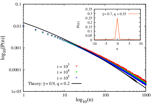
with $|R(n)|<\{(K/q^{*})^{2}\Gamma(\mu+1)/\pi\sin(\pi\mu/2)\}|n|^{-1-2\mu}$. The walker is thus power-law localized, with exponent $-(1+\mu)$ at large $|n|$. Fig.(5) shows the good agreement between $P_{n}$ obtained from numerical inversion and simulations at $\mu=0.5$.

The robustness of the localization phenomenon can be probed by incorporating resource depletion and refreshing in rule (b). Let us assume that the inhomogeneity becomes empty each time the walker leaves it ($\gamma$ set to $0$), and then recovers ($0\rightarrow\gamma$) at a later time with rate $\tau$. Fig. 3-left displays a simulation curve of $P_{0}$ for $\tau=0.1$, whose shape is similar to that of the base model.

In summary, we have demonstrated with a solvable model that random walkers with resetting and memory are able to learn by reinforcement and adapt to features of their environments. Adaptation is revealed through a localization phase transition which emerges around a trapping site. The localized walker asymptotically behaves as if it reset to the trapping site solely, with an effective resetting rate that vanishes at criticality. Apart from applications in cognition and ecology, the results presented here could motivate applications for pattern recognition, the tracking of mobile objects, or for developing algorithms that solve difficult optimization problems. Our study also establishes a long sought formal analogy between the localization of path-dependent random walks and that of waves in disordered media [20]. Despite the radically different physical nature, non-Markovian stochastic processes with resetting may prove useful for studying Anderson transitions.

DB and LG acknowledge support from the Max Planck Institute for the Physics of Complex Systems and its Advanced Study Group “Anomalous diffusion in foraging”. DB acknowledges support from DGAPA-PAPIIT Grant IN105015, and LG from EPSRC grant EP/I013717/1. We thank A. Aldana, M. Aldana, J. Cardy, F. Leyvraz, and G. G. Naumis for fruitful discussions.

Supplemental Material

References

- [1] E. Kagan and I. Ben-Gal, Search and foraging : individual motion and swarm dynamics (CRC Press, Boca Raton, Florida, 2015).
- [2] G. M. Viswanathan, M. G. E. da Luz, E. P. Raposo, and H. E. Stanley, The Physics of foraging (Cambridge, Cambridge, 2011).
- [3] O. Bénichou, C. Loverdo, M. Moreau, and R. Voituriez, Rev. Mod. Phys. 83, 81 (2011).
- [4] P. Turchin, Quantitative analysis of movement.(Sunderland, MA. Sinauer Associates Inc, 1998).
- [5] E. A. Codling, M. J. Plank, and S. Benhamou, J. R. Soc. Interface 5, 813 (2008).
- [6] Cai, Yifan and Simon X. Yang, in it Intelligent Control and Automation (WCICA), 11th World Congress on IEEE (2014).
- [7] J. A. Merkle, D. Fortin, J. M. Morales, Ecol. Lett. 17, 12294 (2014)
- [8] C. Song, T. Koren, P. Wang, and A.-L. Barabási, Nature Phys. 6, 818 (2010).
- [9] X.-W. Wang, X.-P. Han, and B.-H. Wang PLoS ONE 9, e84954 (2014).
- [10] D. Boyer, M. C. Crofoot, and P. D. Walsh, J. R. Soc. Interface 9, 842-847 (2012).
- [11] J. M. Morales, D. T. Haydon, J. Frair, K. E. Holsinger, and J. M. Fryxell, Ecology 85, 2436 (2004).
- [12] Theraulaz, G. and Bonabeau, E., Artificial Life, 5(2) , 97-116 (1999).
- [13] W. F. Fagan et al., Ecol. Lett. 16, 1316 (2013).
- [14] Bonabeau, Eric and Dorigo, Marco and Theraulaz, Guy, Swarm intelligence: from natural to artificial systems, (Oxford University Press, 1999).
- [15] Schacter, D.L., J. Cogn. Neurosci., 4(3), 244???256 (1992).
- [16] B. van Moorter et al., Oikos 118, 641 (2009).
- [17] D. Boyer, P. D. Walsh, Phil. Trans. R. Soc 368, 5645-5659 (2010).
- [18] T. Gueudré, A. Dobrinevski, and J.-P. Bouchaud, Phys. Rev. Lett. 112, 050602 (2014).
- [19] R. Pemantle, Prob. Surv. 4, 1 (2007).
- [20] T. Spencer, In: E. Abrahams, Ed. 50 years of Anderson localization (World Scientific, 2010), pp. 327-345.
- [21] J. G. Foster, P. Grassberger and M. Paczuski, New J. Phys. 11, 023009 (2009).
- [22] A. O. Gautestad and I. Mysterud, Ecol. Complex. 3, 44 (2006).
- [23] L. Brger, B. D. Dalziel, and J. M. Fryxell, Ecol. Lett. 11, 637 (2008).
- [24] C. E. Vincenot et al., Ecol. Compl. 22, 139 (2015).
- [25] D. Luce (1959). Individual choice behavior (John Wiley Sons, New York, 1959).
- [26] P. Wlfle and D. Vollhardt, In: E. Abrahams, Ed. 50 years of Anderson localization (World Scientific, 2010), pp. 43-71.
- [27] S. C. Manrubia and D. H. Zanette, Phys. Rev. E 59, 4945 (1999).
- [28] M. R. Evans and S. N. Majumdar, Phys. Rev. Lett. 106, 160601 (2011).
- [29] M. R. Evans and S. N. Majumdar, J. Phys. A: Math. Theor. 44, 435001 (2011).
- [30] M. R. Evans and S. N. Majumdar, J. Phys. A: Math. Theor. 47, 285001 (2014).
- [31] L. Kusmierz, S. N. Majumdar, S. Sabhapandit, and G. Schehr, Phys. Rev. Lett. 113, 220602 (2014).
- [32] S. Eule and J. J. Metzger, New J. Phys. 18, 033006 (2016).
- [33] S. N. Majumdar, S. Sabhapandit, G. Schehr, Phys. Rev. E 91, 052131 (2015).
- [34] A. Pal, A. Kundu, and M. R. Evans, J. Phys. A: Math. Theor. 49, 225001 (2016).
- [35] A. Pal and S. Reuveni, Phys. Rev. Lett. 118, 030603 (2017).
- [36] V. Méndez and D. Campos, Phys. Rev. E 93, 022106 (2016).
- [37] D. Boyer, C. Solis-Salas, Phys. Rev. Lett. 112, 240601 (2014).
- [38] S. N. Majumdar, S. Sabhapandit, G. Schehr, Phys. Rev. E 92, 052126 (2015).
- [39] D. Boyer, M. R. Evans, and S. N. Majumdar, J. Stat. Mech. 023208 (2017).
- [40] D. Boyer, I. Pineda, Phys. Rev. E 93, 022103 (2016).
- [41] W. Feller, An Introduction to Probability Theory and its Applications (Wiley, New York, 2008).
- [42] See Supplemental Material for calculation details, which includes Ref. [43].
- [43] Gradshteyn, I. S. and Ryzhik, I. M., Table of integrals, series, and products, Eighth ed., (Elsevier/Academic Press, Amsterdam, 2015).
- [44] Since the first passage properties of the model with are not known, a full understanding of the role of is lacking. Due to the slow anomalous diffusion, the walker should eventually find the origin and localize around it. Another scenario could be that some trajectories localize whereas others don’t (e.g., if they do not find the origin). Even in such case, as the localized states are described by Eqs. (4)-(5), our conclusions would not change.
- [45] G. Samoradnitsky and M. S. Taqqu, Stable Non-Gaussian Random Processes: Stochastic Models with Infinite Variance (Champan & Hall, London, 1994).
- [46] G. H. Weiss, Aspect and Applications of the Random Walk (Elseiver, Amsterdam, 1994).
- [47] D. Vollhardt and P. Wolfle, Phys. Rev. Lett. 48, 699 (1982).
- [48] D. Vollhardt and P. Wolfle, Phys. Rev. B 22, 4666 (1980).
- [49] N. Goldenfeld, Lectures on phase transitions and the renormalization group (Addison-Wesley, Reading, 1992).
- [50] L. Kusmierz and E. Gudowska-Nowak, Phys. Rev. E. 92, 052127 (2015).
- [51] S. Kotz, I. V. Ostrovskii, and A. Hayfavi, J. Math. Anal. Appl. 193, 353 (1995).