Modeling Between-Study Heterogeneity for Improved Replicability in Gene Signature Selection and Clinical Prediction
Abstract
In the genomic era, the identification of gene signatures associated with disease is of significant interest. Such signatures are often used to predict clinical outcomes in new patients and aid clinical decision-making. However, recent studies have shown that gene signatures are often not replicable. This occurrence has practical implications regarding the generalizability and clinical applicability of such signatures. To improve replicability, we introduce a novel approach to select gene signatures from multiple datasets whose effects are consistently non-zero and account for between-study heterogeneity. We build our model upon some rank-based quantities, facilitating integration over different genomic datasets. A high dimensional penalized Generalized Linear Mixed Model (pGLMM) is used to select gene signatures and address data heterogeneity. We compare our method to some commonly used strategies that select gene signatures ignoring between-study heterogeneity. We provide asymptotic results justifying the performance of our method and demonstrate its advantage in the presence of heterogeneity through thorough simulation studies. Lastly, we motivate our method through a case study subtyping pancreatic cancer patients from four gene expression studies.
1Department of Biostatistics, Gillings School of Global Public Health
2Lineberger Comprehensive Cancer Center
3 Department of Surgery
4 Department of Pharmacology
University of North Carolina at Chapel Hill
Chapel Hill, NC, U.S.A.
Naim U. Rashid naim@unc.edu,
Quefeng Li quefeng@email.unc.edu,
Jen Jen Yeh jen_jen_yeh@med.unc.edu, and
Joseph G. Ibrahim ibrahim@bios.unc.edu
Keywords: Generalized linear mixed models, microarray, penalized likelihood, prediction, RNA-seq.
1 Introduction
In the genomic era, gene signatures are often utilized to subtype cancer patients, determine treatment, and predict response to therapy (Golub et al., 1999; Swisher et al., 2012; Sotiriou and Piccart, 2007). Such signatures are defined as the collection of one or more genes whose expression has validated specificity with respect to a particular clinical outcome (Chibon, 2013). These signatures are often incorporated into statistical or computational models for predicting clinical outcome in future patients. For these reasons, gene signature selection and subsequent clinical prediction is of significant interest in cancer research.
However, several problems exist with the application of such signatures. For example, inconsistency in gene signature selection is common in published biomedical articles. Gene signatures identified in one article often show little or even no overlap with the ones identified in another article (Waldron et al., 2014). In addition, models based upon these signatures have shown variable accuracy in predicting outcomes in new clinical studies (Sotiriou and Piccart, 2007; Waldron et al., 2014), or estimate contradictory effects of individual genes (Swisher et al., 2012). This lack of replicability presents natural questions towards the generalizability and reliability of utilizing such gene signatures for clinical prediction (Sotiriou and Piccart, 2007).
A number of factors contribute to such a lack of replicability. For example, studies with small sample size have been shown to lack power in selecting gene signatures (Sotiriou and Piccart, 2007) and have low prediction accuracy in new studies (Waldron et al., 2014). Variation in the prevalence of the clinical outcome also affects replicability. Lusa et al. (2007) demonstrate that gene signatures derived from studies with low frequencies of certain molecular subtypes are less likely to accurately predict molecular subtype in new patients. Study-specific factors such as variation in laboratory conditions or clinical protocols may also introduce additional variation in the effects of individual genes.
Differences in data pre-processing is another source. For example, the prediction accuracy of certain classifiers has been shown to be sensitive to the type of normalization method in the pre-processing step (Lusa et al., 2007; Paquet and Hallett, 2015). New datasets must be normalized to the training data prior to its application for prediction to correct for technical biases. However, prior work has shown that this procedure results in “test-set bias”, where predictions may change due to the samples in the test set or the normalization approach used (Patil et al., 2015). Sophisticated procedures have been developed for microarrays to avoid test-set bias, but still require expression data to come from the same type of microarray chip (McCall et al., 2010). If the new study utilizes a different platform, it is even harder to apply and validate the prediction model. For example, next generation sequencing data measures gene expression on a different scale (positive integer counts) relative to microarray data (continuous measurements). Such a difference typically makes methods developed for one platform not applicable to the other (Glas et al., 2006).
To improve replicability, various statistical methods have been developed to integrate data from multiple studies (horizontal integration) to reach a consensus conclusion. Richardson et al. (2016) give a comprehensive review of recent developments in this field. Addressing between-study heterogeneity is critical in horizontal data integration, as data from different studies come from different cohorts, platforms and bio-samples. Several methods (Li et al., 2011; Li et al., 2014) have been developed to account for between-study heterogeneity in horizontal data integration. However, these methods mainly focus on variable selection instead of prediction.
Motivated by a case study in subtyping pancreatic cancer patients, we develop a new horizontal integration method that selects gene signatures from multiple datasets and accounts for between-study heterogeneity in variable effects. We apply a rank-based transformation based upon gene pairs to the raw expression data, facilitating data integration from multiple studies. We note that some care needs to be taken when merging data from different expression platforms. More details of this rank-based transformation will be discussed in Section 3. Given the transformed data, we utilize a penalized Generalized Linear Mixed Model (pGLMM) to select predictors with study-replicable effects and account for between-study heterogeneity. In particular, we assume the effect of each predictor to be random among different studies. We design a penalty function to select predictors with nonzero fixed effects in addition to those with non-zero variance across studies. We propose to only use predictors with nonzero fixed effects to predict outcome in new subjects, as their effects are replicable in multiple studies. Through simulation and case studies, we demonstrate that in the presence of between-study heterogeneity, our proposed method can result in better prediction performance than other commonly used strategies, especially when the heterogeneity is large. Moreover, as we use the transformed data as predictors in the pGLMM, our method aims to select gene pairs instead of individual genes for prediction.
2 Data
Pancreatic Ductal Adenocarcinoma (PDAC) remains a lethal disease with a 5-year survival rate of 4. A key hallmark of PDAC is the low tumor cellularity of patient samples, which makes capturing precise tumor-specific molecular information difficult. Due to this fact, genomic subtyping of PDAC to inform treatment selection has been limited.
In a recent study, Moffitt et al. (2015) identified genes that are expressed solely in pancreatic tumor cells. Based upon these tumor-specific genes, two novel tumor subtypes (‘basal-like’ and ‘classical’) were identified and validated. Subtypes were found to be prognostic, in that patients with basal-like tumors had significantly worse median survival than patients with classical tumors. Lastly, it was found that tumor-specific genes from the basal-like subtype also define a similar basal-like subtype in breast and bladder cancers, suggesting a common basal-like genomic profile shared across cancer types. This study represented the largest investigation of primary and metastatic PDAC gene expression thus far and provided new insights into the molecular composition of PDAC. These insights may be used to make tailored treatment recommendations.
Given these promising results, methods are needed to robustly predict basal-like subtype. However, existing datasets with basal-like subtypes in PDAC are limited. Therefore, we utilize the gene expression data from Moffitt et al. (2015) in addition to recently published PDAC RNA-seq data to train a PDAC subtype classifier. Of the three datasets examined in Moffitt et al. (2015), two are single-channel microarrays (UNC PDAC, UNC Breast Cancer) and one is RNA-seq (TCGA Bladder Cancer). Since the publication of Moffitt et al. (2015), an additional PDAC RNA-seq dataset from The Cancer Genome Atlas (TCGA) has become available and will also be utilized for training (Weinstein et al., 2013). Expression measurements from each RNA-seq dataset is summarized in terms of Fragments Per Kilobase of transcript per Million mapped reads (FPKM), a measurement that accounts for both transcript length and the number of mapped reads within a sample (Trapnell et al., 2010). This allows for easier comparison of expression measurements across genes and samples within an RNA-seq study. More modern RNA-seq measurements, such as Transcripts Per Million (TPM, Patro et al. (2017)) may also be utilized but were not available from Moffitt et al. (2015). Basic information regarding each dataset is provided in Table 1. Each microarray dataset was normalized as described in Moffitt et al. (2015).
We wish to harness the above datasets to select gene signatures that are predictive of the basal-like subtype. However, the datasets arise from various expression platforms and therefore have different scales for their expression measurements. Furthermore, the datasets have been separately pre-normalized. For these reasons, external validation and comparison of basal-like subtype prediction models trained separately on each dataset is challenging. In addition, integrating datasets to train a single prediction model and select study-consistent variables is difficult, given various expression platforms and states of pre-processing. The between-study heterogeneity in gene effects may also impact the selection and estimation of study-consistent variables for subtype prediction.
Motivated by these issues, we propose a novel data integration approach to facilitate between-study comparisons and merging of samples in Section 3. We also introduce a high dimensional pGLMM to select variables that are study-consistent while accounting for between-study heterogeneity in their effects. We compare our method with several common strategies for gene signature selection and subtype prediction using the data in Table 1, and summarize the results in Section 7.
| Dataset | Platform | Sample Size | Gene Set Size | of Basal-like | Pre-normalized? |
|---|---|---|---|---|---|
| UNC PDAC | Microarray | 228 | 19749 | 40 | Yes |
| UNC Breast Cancer | Microarray | 337 | 17631 | 26 | Yes |
| TCGA Bladder Cancer | RNA-seq | 223 | 20533 | 47 | No |
| TCGA PDAC | RNA-seq | 150 | 20531 | 43 | No |
3 Methods
We consider integrating data from independent studies. For simplicity, we assume there are subjects in each study and the total sample size . In the -th study for , let be the vector of independent responses, be the -dimensional vector of predictors, and . Suppose the conditional distribution of given belongs to the canonical exponential family, having the following density function up to an affine transformation that
| (1) |
where is a constant that only depends on , is the dispersion parameter, is a known link function, and the linear predictor
| (2) |
such that is the -dimensional vector of fixed effects, is the -dimensional vector of unobservable random effects, is a -dimensional subvector of , and is a lower triangular matrix. We assume are independent and identically distributed from a general distribution with density . A common choice of is the multivariate normal distribution and . In addition, we assume that and . The random component in the linear predictor has . We allow some rows of to be identically zero, which implies that the effects of corresponding covariates are fixed across the studies. We consider the high dimensional setting for which , , and they both can grow with . We use the subscript to denote such a dependence on .
Similar to Chen and Dunson (2003) and Ibrahim et al. (2011), we reparameterize the linear predictor as
| (3) |
where is a vector consisting of nonzero elements of the -th row of , , and is the matrix that transforms to , i.e. . We define the vector of parameters and assume the true value of is such that , where is the total log-likelihood from the studies. While the linear predictor is indeed a function of the parameter , we suppress its dependence on for the sake of notational simplicity. In addition, we abbreviate as , the value of the linear predictor when the parameters are taken at their true values. As proposed in the above, we would like to identify the set
Let be the cardinality of set , be the cardinality of set , , and be the dimension of the whole problem. In this paper, we consider the case that , , , and change with sample size , but remains fixed.
In order to recover the set , we propose to solve the following penalized likelihood problem:
| (4) |
where , is the observed log-likelihood from the -th dataset such that , and are some penalty functions, and and are positive tuning parameters. Since (4) is a likelihood based method, we may allow the responses to be of different types. We choose and as general folded-concave penalty functions that satisfy condition 8 in Lemma 1 in the Supplementary Material. Examples of such functions include the penalty, the SCAD penalty (Fan and Li, 2001) and the MCP penalty (Zhang, 2010). The penalization on is done in a groupwise manner (Yuan and Lin, 2006), namely we regard elements in as a group and penalize its -norm. Elements of the corresponding estimator will be either all zero or all nonzero. If , the corresponding variable’s effect is regarded as fixed across studies. The selection of such variables (i.e. ) enables us to determine which predictors have non-zero fixed effects. We postulate that accounting for study-level heterogeneity will reduce the bias in fixed effects estimates.
In most applications, we recommend setting and let the algorithm determine which variables should be regarded as fixed effects. However, if we know that some variables can be treated as fixed effects based on prior knowledge, we only need to impose the penalty on the other variables. Based on selections in , we only use predictors with nonzero fixed effects for prediction.
Compared to the existing literature on pGLMMs (Bondell et al., 2010; Ibrahim et al., 2011), our paper is new in the following perspectives. First, we deal with a much larger dimension compared to existing articles. In our application, and can both be greater than 50, yielding at least possible models to be chosen from, whereas the existing articles only consider and in Ibrahim et al. (2011) and in Bondell et al. (2010). In particular, large values of increase the computational complexity of the problem, as the likelihood in (4) involves an integral of dimension . To solve such a large-scale problem, a new algorithm is developed to estimate the pGLMM. More details are given in Section 4. In addition, we give a high-dimensional asymptotic result in Theorem 1 allowing both and diverge with , while the theory in Ibrahim et al. (2011) requires and to be fixed.
Next, we introduce a technique to facilitate data integration over different studies. The motivation is that even though the raw values of gene expression may be on different scales in different studies, their relative magnitudes can be preserved by ranks. Therefore, we propose to use some rank-derived quantities as predictors in models (1) and (2), instead of the raw values. We use a variant of the Top Scoring Pair (TSP) approach (Leek, 2009; Patil et al., 2015; Afsari et al., 2015).
Suppose there are common genes in all studies. We enumerate gene pairs , where is the raw expression of gene for subject in study and is defined similarly. For each gene pair , the TSP is an indicator representing which gene of the two has higher expression in subject . Such binary indicators are then used as the predictors in (1) and (2). In other words, consists of binary variables.
We view such binary variables as “biological switches” indicating how pairs of genes are expressed relative to some clinical outcome. TSPs were originally proposed in the context of binary classification (Afsari et al., 2014). We find that this representation of the original data is also appealing for integrative analysis. First, the TSP only depends on the ranks of raw gene expression in a sample. Hence, it is invariant to monotone transformations of raw values. As a result, it is less sensitive to various normalization procedures of data pre-processing. (Afsari et al., 2014; Patil et al., 2015; Leek, 2009). Second, it simplifies data integration over different studies. The raw gene expression values may not be directly comparable. After converting them into binary scores, data from different studies can be pooled together without the need for between-sample or cross-study normalization. Prediction in new patients is also simplified, as normalizing new patient data to the training set is no longer necessary.
In general, we wish to select gene pairs that are consistent in their relationship with subtypes across multiple studies. An ideal gene pair is such that one gene in the pair has higher expression than the other gene in one subtype, lower expression in the other subtype, and has this flip replicated across many subjects. Each gene in the pair should ideally be differentially expressed between subtypes. Such ideal gene pairs are less likely to be observed purely due to technical biases, as this flip in expression is specific to subtype and is also replicated across many subjects. Indeed, many recent publications utilizing gene pair-based approaches have shown high accuracy and robustness in their validation datasets, reflecting this point (Afsari et al., 2015; Shen et al., 2017; Afsari et al., 2014; Leek, 2009; Kagaris et al., 2018; Patil et al., 2015).
However, some care needs to be taken when merging gene pairs generated from different platforms, especially when merging microarray data with data from other platforms such as RNA-seq. For microarrays, it is known that differences in absolute expression between certain genes may not correlate with differences in measured probe-level expression. Therefore, merging microarray data with other platforms may reduce the sensitivity to detect such ideal gene pairs. As a result, our gene-pair approach is more applicable when data come from the same or similar platforms. It is also preferable to utilize more modern expression platforms (such as RNA-seq), as well techniques that correct for GC content and other biases in gene expression measurement (Patro et al., 2017), as these approaches may improve the correlation between measured and true expression of genes. Lastly, our gene pair approach is predicated on the fact that the genes must also have overlapping expression ranges. This is commonly observed in our real data application candidate gene set, but may not always be the case. When the expression ranges of two genes do not overlap, the corresponding TSP will not flip with respect to subtype across patients, and would therefore would be uninformative for prediction.
4 MCECM Algorithm
Since the observed likelihood involves intractable integrals, we utilize a Monte Carlo Expectation Conditional Minimization (MCECM) algorithm for solving (4) (Garcia et al., 2010). Denote the complete and the observed data for study by and , respectively, and the entire complete and observed data by and , respectively. Let . At the -th iteration, given , the E-step is to evaluate the penalized Q-function, given by
| (5) | |||||
| (6) |
where , and
Because these integrals are often intractable, we approximate these integrals by taking a Markov Chain Monte Carlo sample of size from the density using a coordinate-wise metropolis algorithm described in McCulloch (1997) with standard normal candidate distribution. This leads to a more efficient performance for larger . Let be the -th simulated value, for , at the -th iteration of the algorithm. The integral in (6) can be approximated as
The M-step involves minimizing
with respect to . Minimizing with respect to is straightforward and can be done using a standard optimization algorithm, such as the Newton-Raphson Algorithm (Rashid et al., 2014). Minimizing with respect to and is done via the coordinate gradient descent algorithm, leading to more efficient performance in larger dimensions.
In particular, we utilize three conditional minimization steps. Prior to minimization, we augment the matrices used in the linear predictor by “filling in” the missing values of with , repeating the rows of the original matrices times and replacing with in each of the repeated rows. This leaves us with , where , and , as well as to match the dimension of , where . We first minimize with respect to given and to obtain using the coordinate gradient descent approach similar to Breheny and Huang (2011) with predictor matrix and offset . We then minimize with respect to given and to obtain using the blockwise gradient descent algorithm (Breheny and Huang, 2015) with serving as an offset. Therefore, elements of the corresponding estimator will be either all zero or all nonzero. If , the -th predictor will be regarded as fixed effect. By separating the penalized estimation of and into two conditional minimization steps, we are able to simplify the variable selection process into a standard variable selection problem for and a group variable selection problem for . Lastly, we minimize with respect to given and to obtain . This minimization is performed using the Newton-Raphson algorithm.
As increases, the dimension of also increases. We utilize an approximation treating the covariance matrix as a diagonal matrix. This approach has been demonstrated to be advantageous for high-dimensional mixed models (Fan and Li, 2012), and also results in greater computational efficiency. This is because the accumulative estimation error in estimating the full covariance matrix for large can be much larger than the bias incurred from utilizing a diagonal covariance matrix.
To ensure that the estimator has good properties, the penalty parameter has to be appropriately selected. Two common criteria are generalized cross validation and BIC (Wang et al., 2007). However, these criteria cannot be easily computed in the presence of random effects, because they are functions of the observed likelihood, which involves intractable integrals. Moreover, it has been shown in Wang et al. (2007) that even in the simple linear model, the generalized cross validation criterion can lead to significant overfitting. Instead, we utilize the ICQ criterion (Ibrahim et al., 2011) to select the optimal by minimizing
where , , is the estimator of from the full model, and is the estimator from the model fitted with a particular . As in the EM algorithm, we can draw a set of samples from for to estimate for any . In higher dimensions, we choose small values for and to approximate . Given the ICQ criterion, we perform a grid search of to find the optimal values.
For the penalty functions, we consider the MCP penalty for both and , which is defined as for and for . Similar to Breheny and Huang (2011), we choose . Other penalties such as the SCAD and the penalties may be utilized. Given the promising performance of the MCP penalty in previous publications, we do not explicitly compare between penalties in this paper.
5 Theory
We first introduce some notation. For two sequences and , we write if ; if ; if for some positive constant . For a -dimensional vector , let denote its sup-norm. Let be a subvector of with indices in the set . For a matrix , let denote the matrix sup-norm. Denote . Let and . For simplicity, we assume the dispersion parameter and . We define the local concavity of the penalty function as
We define a neighborhood of as , where for some , , , and .
The main result in Theorem 1 implies that the estimator asymptotically recovers and gives a uniform consistent estimator of .
Theorem 1.
Assume conditions (C1)-(C8) as shown in the Supplementary Material hold. If ,
for and
, where ,
, and
, there exists a sufficiently large
positive constant such that with probability greater
than , it holds that
(a) .
(b) , where .
The convergence rate in statement (b) depends on the minimal signal , the dimensionality , the sparsity measurement and the penalty function . In general, the larger is and the smaller and are, the faster converges. The optimal rate can be as close as a root- rate.
In Theorem 1, it is feasible to choose proper tuning parameters and to satisfy all requirements. For example, if the penalty is used, and we assume is bounded away from 0, we only need to choose and such that for some and . As long as and , there exists a feasible region for and . In practice, we tune the optimal and using methods described in Section 4.
6 Simulation Studies
6.1 Oracle setting
We first examine the oracle setting where the variables relevant to the outcome are known apriori. We demonstrate the performance of our method in comparison to some common strategies to estimate variable effects from multiple datasets. The first strategy is the traditional study-by-study analysis approach, where variable effects are estimated separately in each individual study. The second strategy is to combine samples from all studies into a single dataset, and then estimate variable effects in a single model. We define a third strategy as a GLMM applied to the merged data, assuming no penalization on the fixed and random effects. To mimic the process of external validation, we utilize the fitted model from each strategy to predict outcomes in an externally simulated dataset. The median absolute prediction error is calculated for each strategy, and is then averaged over simulations. We assess each strategy’s performance in terms of the bias of the estimated coefficients as well as the prediction accuracy under external validation. We will later examine the variable selection performance under similar conditions when the set of relevant variables is unknown apriori.
Specifically, we generate binary responses representing cancer subtype from a random effects logistic regression model with two predictors and an intercept. A range of sample sizes, number of studies, magnitudes of variable effects, and levels of between-study heterogeneity are to be inspected. For study , we generate the binary response , such that where , and , where controls between-study heterogeneity. To simulate imbalanced sample sizes, we allocate samples to study and evenly distribute the remaining samples to the remaining studies. We perform simulations for , , , for moderate predictor effect, and for strong predictor effect. For each , we denote the vector of predictors pertaining to subject as , where we assume , . We also assume a random intercept and random slope for each predictor by setting . The external validation set of 100 samples is generated under the same conditions as the training set to produce and .
For the first strategy (IND), we apply a logistic regression model to each of the datasets and calculate , the predicted probability of , using and the estimated coefficients from each model. For the second strategy (GLM), we apply a logistic regression model to the merged dataset to obtain . For our method (GLMM), we apply a random effects logistic regression model to the merged dataset to obtain the estimated fixed effect coefficients, assuming a random slope for each predictor. Here, only the estimated fixed effect coefficients are used to obtain . In all of the above regression models, we assume the relevant predictors are known to us and only use them in the model. The median absolute prediction error for each strategy is calculated as , where varies in the validation set. For the first strategy, is averaged across the studies.
We first illustrate the results of a single simulation in Figure 1. In this scenario, we simulate five studies of a total of 500 samples assuming moderate variable effects and high between-study heterogeneity, i.e., we choose , , , . Applying the first strategy to the data illustrates the significant study-to-study variation in the estimated coefficients (Figure 1, left panel). This variation is also observed for the study-level absolute prediction errors in the simulated external validation set (Figure 1, right panel). In this setting, researchers using Study 3 would estimate a strong association between each predictor and the response, and may further conclude that their model performs well in the validation set. However, researchers using Study 1 may conclude otherwise due to the between-study heterogeneity in variable effects. Combining data in the second strategy results in smaller prediction errors compared with the first strategy. This observation is in line with the prior findings suggesting that combining data results in better estimation and prediction (Waldron et al., 2014). However, accounting for heterogeneity further improves the median absolute prediction error.
Our full simulation results are presented in Tables 2 and 3, where we average results over 100 simulations per condition. Several trends are apparent from these results, reflecting our illustration from Figure 1. First, combining data from multiple studies results in an reduction of the median absolute prediction error (, ) compared with models trained on individual studies (); see Table 2. We also find that the relative prediction accuracy of the GLMM improves more when the simulated heterogeneity and the number of studies increase. This is due to an increased bias by the GLM when and increase. Also, differences in prediction accuracy between the two strategies become more apparent as the strength of the predictor effects increases (Table 3). Lastly, the bias of the estimated coefficients by the GLMM decreases as and increase, as more data are available to estimate and . In all, combining datasets in strategies two and three leads to better prediction accuracy and accounting for between-study heterogeneity via our method further improves the performance.
These observations show that even in the oracle setting where the relevant predictors are known, accounting between-study heterogeneity has important consequences in model estimation and prediction. We assume in our simulations that the training and validation sets are generated from the same population. We show that even without other complicating factors, between-study heterogeneity can still impact the accuracy and replicability of common approaches such as strategies one and two. While we utilize normally-distributed predictors in our simulations, the impact of between-study heterogeneity will generally apply to variables from any distribution. In the next section, we show that heterogeneity presents additional problems in variable selection when important variables are unknown.
| 100 | 2 | 0.5 | 1.03 | 1.06 | 0.90 | 1.03 | 0.33 | 0.34 | 0.39 |
|---|---|---|---|---|---|---|---|---|---|
| 1 | 1.11 | 1.06 | 0.84 | 0.81 | 0.38 | 0.40 | 0.43 | ||
| 2 | 1.01 | 0.97 | 0.76 | 0.49 | 0.42 | 0.43 | 0.46 | ||
| 5 | 0.5 | 1.14 | 1.15 | 0.95 | 0.93 | 0.34 | 0.35 | 0.39 | |
| 1 | 1.12 | 0.98 | 0.77 | 0.74 | 0.40 | 0.42 | 0.43 | ||
| 2 | 1.22 | 1.06 | 0.53 | 0.49 | 0.45 | 0.47 | 0.48 | ||
| 10 | 0.5 | 1.15 | 1.20 | 0.93 | 0.96 | 0.33 | 0.35 | 0.39 | |
| 1 | 1.07 | 1.01 | 0.73 | 0.67 | 0.38 | 0.41 | 0.43 | ||
| 2 | 1.02 | 0.87 | 0.40 | 0.40 | 0.43 | 0.47 | 0.47 | ||
| 500 | 2 | 0.5 | 1.05 | 1.00 | 1.01 | 0.95 | 0.35 | 0.36 | 0.39 |
| 1 | 0.93 | 1.03 | 0.82 | 0.79 | 0.39 | 0.42 | 0.43 | ||
| 2 | 0.90 | 0.79 | 0.63 | 0.55 | 0.44 | 0.46 | 0.47 | ||
| 5 | 0.5 | 0.99 | 1.04 | 0.89 | 0.90 | 0.33 | 0.36 | 0.41 | |
| 1 | 0.99 | 0.93 | 0.73 | 0.63 | 0.36 | 0.41 | 0.44 | ||
| 2 | 0.94 | 0.92 | 0.41 | 0.40 | 0.42 | 0.47 | 0.48 | ||
| 10 | 0.5 | 0.99 | 1.04 | 0.90 | 0.94 | 0.34 | 0.36 | 0.39 | |
| 1 | 1.09 | 0.99 | 0.77 | 0.69 | 0.37 | 0.40 | 0.42 | ||
| 2 | 0.94 | 0.97 | 0.49 | 0.47 | 0.43 | 0.47 | 0.47 |
| 100 | 2 | 0.5 | 2.11 | 2.09 | 1.96 | 1.88 | 0.14 | 0.16 | 0.26 |
|---|---|---|---|---|---|---|---|---|---|
| 1 | 2.22 | 2.11 | 1.72 | 1.65 | 0.16 | 0.21 | 0.30 | ||
| 2 | 1.79 | 2.30 | 1.08 | 1.28 | 0.30 | 0.35 | 0.41 | ||
| 5 | 0.5 | 2.18 | 2.31 | 1.89 | 1.98 | 0.16 | 0.17 | 0.26 | |
| 1 | 2.12 | 2.21 | 1.52 | 1.47 | 0.19 | 0.22 | 0.31 | ||
| 2 | 1.91 | 1.92 | 0.85 | 0.85 | 0.27 | 0.32 | 0.38 | ||
| 10 | 0.5 | 2.25 | 2.31 | 1.88 | 1.86 | 0.13 | 0.17 | 0.26 | |
| 1 | 2.07 | 2.26 | 1.39 | 1.51 | 0.17 | 0.24 | 0.32 | ||
| 2 | 2.26 | 2.12 | 0.98 | 0.77 | 0.28 | 0.38 | 0.40 | ||
| 500 | 2 | 0.5 | 2.04 | 1.98 | 1.97 | 1.93 | 0.15 | 0.17 | 0.26 |
| 1 | 1.93 | 1.95 | 1.66 | 1.60 | 0.20 | 0.26 | 0.32 | ||
| 2 | 2.10 | 1.96 | 1.54 | 1.18 | 0.26 | 0.36 | 0.39 | ||
| 5 | 0.5 | 2.09 | 2.00 | 1.92 | 1.85 | 0.12 | 0.16 | 0.29 | |
| 1 | 2.02 | 1.89 | 1.54 | 1.44 | 0.18 | 0.25 | 0.36 | ||
| 2 | 1.88 | 1.89 | 0.89 | 0.87 | 0.25 | 0.36 | 0.41 | ||
| 10 | 0.5 | 2.01 | 1.98 | 1.85 | 1.85 | 0.15 | 0.17 | 0.26 | |
| 1 | 1.93 | 1.91 | 1.41 | 1.40 | 0.18 | 0.25 | 0.31 | ||
| 2 | 1.81 | 1.83 | 0.88 | 0.90 | 0.27 | 0.36 | 0.40 |


6.2 Non-oracle setting
We again assume that only two variables are relevant to the outcome, but now are unknown apriori. We aim to select these variables from a set of variables and utilize them to predict outcomes in an external dataset. In our simulation, we assume the effects of the remaining variables are zero in all studies. We simulate our data the same way as in the previous section, except we now generate . We assume . We consider or 50, , and or 10. Simulation results for these scenarios are given in Tables 4 and 5.
We examine three strategies for selecting and estimating the effects of the relevant variables. For the first strategy (IND), we apply a penalized logistic regression model separately in each study to select relevant variables. For the second strategy (GLM), we merge samples from all studies, and then apply the penalized logistic regression to select relevant variables. Lastly, we apply our method (GLMM) to the merged dataset. The BIC is used to select the optimal tuning parameters for the first two methods. The optimal tuning parameters of our method are obtained via a grid search based on the ICQ. In all methods, we choose the MCP penalty. Two metrics assessing variable selection performance are presented in Tables 4 and 5. We denote as the true positives, i.e., the number of correctly selected variables with true non-zero effects; and as the false positives, i.e., the number of incorrectly selected variables with true zero effect.
In the low dimensional setting of , our method is most advantageous when the heterogeneity is high and the variables’ effects are moderate (Table 4). In general, strategy two selects fewer true positives but more false positives compared with our method. We also find that the first strategy results in the fewest true positives with the greatest false positives. Its performance worsens when and increase. This is due to the smaller per-study sample size when increases, as well as the greater chance to have small simulated effects at larger . Similar to the previous section, we observe that the first two strategies perform worse than our method in estimation. These results also apply in the high dimensional setting of . In this scenario, the is slightly higher than in certain settings. But the GLMM has better sensitivity in selecting true positives and prediction performance.
Overall, we find that combining datasets improves the variable selection compared with the study-by-study analysis. We also find that accounting for heterogeneity in our method can further improve variable selection, reduce bias, and reduce prediction error. In the non-oracle setting where the relevant variables are unknown, the prediction errors are generally larger than the ones in the oracle case. This is due to the uncertainty of variable selection as well as the bias introduced by penalization.
| 500 | 10 | 5 | 1 | 0.96 | 1.05 | 0.63 | 0.68 | 1.80 | 0.14 | 1.75 | 0.34 | 0.54 | 1.40 | 0.39 | 0.42 | 0.44 |
|---|---|---|---|---|---|---|---|---|---|---|---|---|---|---|---|---|
| 2 | 1.16 | 1.33 | 0.60 | 0.57 | 1.44 | 0.15 | 1.34 | 0.27 | 0.49 | 1.40 | 0.45 | 0.48 | 0.48 | |||
| 10 | 1 | 0.99 | 0.89 | 0.67 | 0.67 | 1.96 | 0.14 | 1.81 | 0.39 | 0.16 | 1.10 | 0.37 | 0.42 | 0.45 | ||
| 2 | 1.11 | 1.20 | 0.39 | 0.57 | 1.71 | 0.13 | 1.53 | 0.26 | 0.11 | 1.20 | 0.45 | 0.47 | 0.49 | |||
| 500 | 50 | 5 | 1 | 1.18 | 1.15 | 0.45 | 0.47 | 1.82 | 0.57 | 1.61 | 0.61 | 0.2 | 0.3 | 0.36 | 0.44 | 0.42 |
| 2 | 1.12 | 1.18 | 0.55 | 0.44 | 1.47 | 0.91 | 1.12 | 0.42 | 0.23 | 1.4 | 0.36 | 0.43 | 0.44 | |||
| 10 | 1 | 1.18 | 1.14 | 0.48 | 0.48 | 1.86 | 0.72 | 1.38 | 0.92 | 0.15 | 1.3 | 0.31 | 0.42 | 0.42 | ||
| 2 | 1.23 | 1.38 | 0.55 | 0.53 | 1.51 | 1.08 | 1.23 | 0.4 | 0.13 | 1.3 | 0.36 | 0.41 | 0.43 |
| 500 | 10 | 5 | 1 | 1.94 | 1.93 | 1.48 | 1.45 | 2.00 | 0.07 | 2.00 | 0.11 | 0.40 | 2.00 | 0.19 | 0.25 | 0.33 |
|---|---|---|---|---|---|---|---|---|---|---|---|---|---|---|---|---|
| 2 | 2.00 | 2.16 | 1.08 | 1.07 | 1.88 | 0.08 | 1.78 | 0.15 | 0.34 | 2.00 | 0.24 | 0.35 | 0.39 | |||
| 10 | 1 | 1.90 | 1.90 | 1.42 | 1.36 | 2.00 | 0.08 | 2.00 | 0.10 | 0.34 | 0.80 | 0.18 | 0.25 | 0.39 | ||
| 2 | 1.83 | 2.00 | 0.95 | 0.94 | 1.97 | 0.11 | 1.80 | 0.23 | 0.22 | 0.90 | 0.28 | 0.39 | 0.44 | |||
| 500 | 50 | 5 | 1 | 2.19 | 2.04 | 1.48 | 1.53 | 2.00 | 0.84 | 1.58 | 1.62 | 0.00 | 0.00 | 0.18 | 0.3 | 0.37 |
| 2 | 2.13 | 1.93 | 1.16 | 0.87 | 1.94 | 2.4 | 1.45 | 1.28 | 0.18 | 1.8 | 0.27 | 0.41 | 0.42 | |||
| 10 | 1 | 2.09 | 2.16 | 1.46 | 1.49 | 2.00 | 1.36 | 1.28 | 2.84 | 0.3 | 0.2 | 0.16 | 0.34 | 0.4 | ||
| 2 | 2.27 | 2.32 | 0.83 | 0.89 | 1.97 | 1.75 | 1.25 | 2.71 | 0.11 | 1.3 | 0.23 | 0.43 | 0.43 |
7 Improved Clinical Subtype Prediction in Pancreatic Cancer via Horizontal Data Integration
Using our described data integration approach, we apply four methods to the four datasets described in Table 1 to predict the ‘basal-like’ subtype in new pancreatic cancer patients. We will show that our method results in better prediction relative to the other methods in the presence of between-study heterogeneity.
To generate the predictors, we first use genes that were deemed to be tumor-specific in Moffitt et al. (2015) and appear in all four studies. Then, we apply the rank transformation described in Section 2 in each dataset, enumerating all possible 45,451 TSPs based on these common genes. To reduce the dimension, we further screen these TSPs by applying a univariate random effects logistic regression model with respect to each TSP, assuming a random slope and a random intercept. We sort the TSPs from largest to the smallest by the marginal likelihood from their corresponding random effects logistic regression model. Then, similar to Afsari et al. (2015), we keep TSPs with larger marginal likelihood and remove TSPs sharing one gene with the higher ranked ones. This reduces potential strong correlation between TSPs sharing same genes (Supplementary Figure 1). After screening, 95 TSPs remain, of which we select the top 50 ones to be used as covariates in the regression model. We aim to determine the best subset of the 50 TSPs for prediction. This results in a total of possible fixed effects models and possible random effects models.
In Figure 2, we represent the top 50 TSPs for each sample in the four studies. Yellow cells indicate that the first gene in the TSP has higher expression than the second gene and the red ones indicate otherwise. It is clear that certain TSPs have variable association with the subtype across studies, i.e., low replicability. Our goal is to select the TSPs that are consistently associated with the subtype across studies while accounting for between-study heterogeneity.

We compare four methods. For the first method, we apply the penalized logistic regression model (pGLM) to each dataset. For the second method, we combine all datasets and run the penalized logistic regression model (pGLMC). For the third method, we run the penalized logistic regression model with random effects on the combined data (pGLMMC). Finally, we run the Meta-Lasso method (Li et al., 2014) on the combined data. For each subject, we assume the response if the subject is of the basal-like subtype and 0 otherwise. The vector is the vector of the screened TSPs as shown in Figure 2. The computational details of the first three methods is the same as described in the simulation study. For the Meta-Lasso method, the coefficients pertaining to the same TSP in multiple studies are treated as a group and the composite group penalty is imposed on each group as in Li et al. (2014), to select the key TSPs. The TSPs selected by Meta-Lasso are defined as the ones that have non-zero estimated coefficients in at least one study. The optimal tuning parameters in Meta-Lasso is determined by the BIC method described in Li et al. (2014).
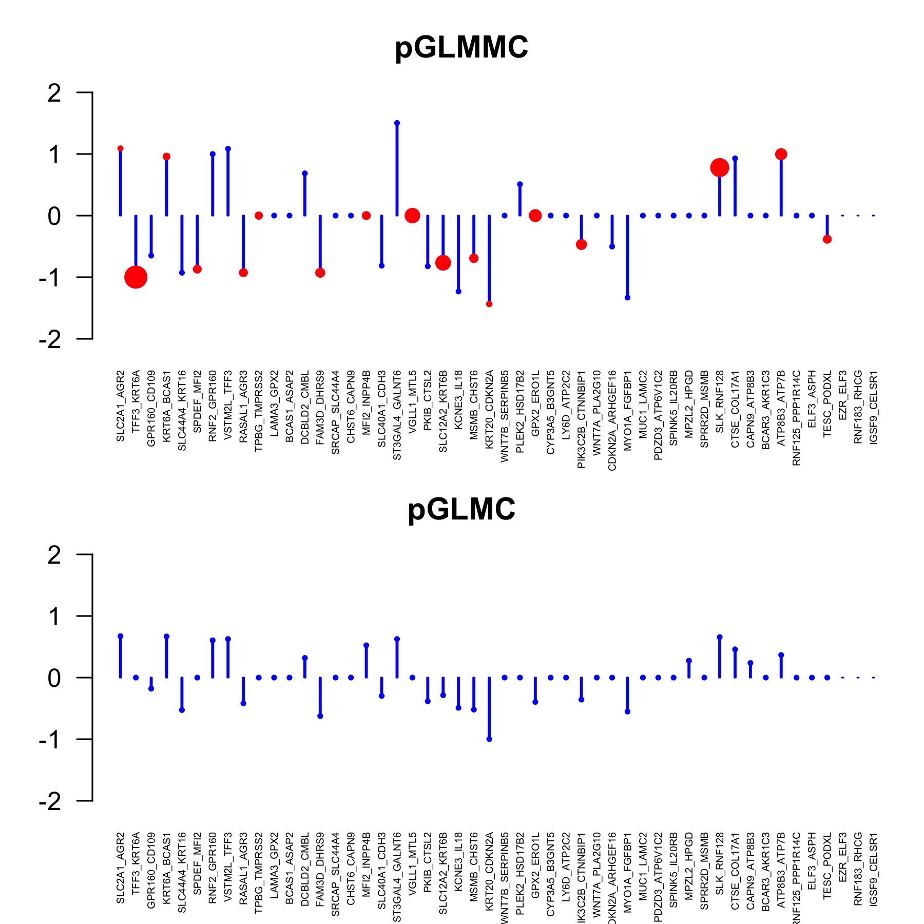
The selected TSPs by the four methods are shown in Figure 3. Not surprisingly, for the pGLM, very different TSPs are selected in different studies. We find that TSPs that are repeatedly selected by the pGLM are also more likely to be selected by the pGLMC. Our method yields larger estimated coefficients than the pGLMC, especially for those TSPs selected by both methods (Figure 4). This mimics findings in our simulation studies that the estimated coefficients given by the pGLMC are biased in the presence of heterogeneity. Moreover, the Meta-Lasso selects very different TSPs resulting in poor replicability.

Next, we evaluate the subtype prediction performance of the four methods. For each method, we hold one dataset out and train the model using the remaining studies. We utilize this procedure to mimic the process of external validation. For the pGLM, an ordinary logistic regression model is fitted to each training study using selected TSPs from Figure 3. The averages of the three predicted probabilities are assigned to subjects in the holdout study. Their absolute prediction errors are then calculated and aggregated from each holdout study. Predictions given by the Meta-Lasso are done similarly using variables selected by itself. For the pGLMC and the pGLMMC, a single logistic model is fitted by combining three training datasets and using their own selected TSPs. The predicted probabilities are then given by such combined models.
Figure 5 shows the prediction errors given by the four methods in each study. From its top left panel, we see that the overall performance of the pGLM and the Meta-Lasso is much worse than the pGLMC and the pGLMMC. These observations reflect the low replicability of predictions from the pGLM and the Meta-Lasso, as the pGLM does not borrow strength across datasets and the Meta-Lasso is a method mainly focused on variable selection. Similar to our simulation studies, our proposed pGLMMC method still performs well, despite the variation of its prediction errors on the TCGA Bladder Cancer dataset is larger than that of the pGLMC. Its median prediction error however is still the best in this study. In addition, as shown in Figure 6, our method is more confident than other methods for classification as most predicted probabilities are either for . In all, combining datasets significantly improves the prediction accuracy. By taking heterogeneity into account, our method performs the best out of all competitors.
In the supplementary material, we provide an alternative screening approach that renders more TSPs and repeat our analysis therein. Our method’s prediction performance is still much better than the pGLM and the Meta-Lasso, albeit it’s only slightly better than the pGLMC (Supplementary Figure 6). This is because the between-study heterogeneity given by the new screening approach is much smaller than the one shown in this section. Lastly, we also train our method on the microarray data only and predict on the RNA-seq data, and vice versa. The prediction performance does not change dramatically (Supplementary Figure 8).


8 Discussion
In this article, we introduce a novel approach accounting for between-study heterogeneity in gene signature selection and clinical prediction. We demonstrate through simulations that approaches ignoring existing between-study heterogeneity have lower prediction accuracy, higher bias, and worse variable selection performance than our method. The common approach of study-by-study analysis shows the worst performance compared with the integrative approaches. Lastly, we show in a case study of pancreatic cancer that our method increases prediction accuracy and replicability, where the data integration is facilitated via a rank-based transformation of the original gene expression data.
These results have some important impact. It is often observed that gene signatures derived from individual studies demonstrate low replicability, even when they pertain to similar clinical outcomes. Our simulation results clearly demonstrate that this is partially due to the heterogeneity among different studies as small sample sizes in individual studies. We have also shown that as the sample sizes of individual studies decreases, the selection sensitivity and prediction performance also deteriorate. Selection sensitivity also decreases when the between-study heterogeneity of a gene’s effect increases. On the other hand, combining data from multiple studies improves variable selection and prediction performance by borrowing strength across studies. However, without taking between-study heterogeneity into account, the naive combination still performs worse than our proposed method. In the absence of between-study heterogeneity, the random effects model reduces to the fixed effects model, and therefore we would expect similar performance. This can be observed in the additional results in the Supplementary Material. Our simulation and case study results clearly show how the effects of the same variable may vary significantly between studies, and how this variability impacts prediction. This explains the lack of replicability observed among published gene signatures.
Finally, we would like to comment that the TSP transformation is one possible way to enable data integration, and that the choice of the transformation is tangential to the penalized GLMM model that we have proposed. In addition, the integration of data from multiple platforms should be taken with care, particularly when merging microarray data with data from other platforms. Finally, our model aims to select TSPs instead of individual genes. The success of the TSP transformation relies on the assumption that the raw gene expression has overlapping ranges. Therefore, as pointed out by one reviewer, it could be possible that some genes that are differentially expressed between subtypes will not be selected by our method.
References
- Afsari et al. (2014) Afsari, B., Braga-Neto, U. M., and Geman, D. (2014). Rank discriminants for predicting phenotypes from RNA expression. The Annals of Applied Statistics 8, 1469–1491.
- Afsari et al. (2015) Afsari, B., Fertig, E. J., Geman, D., and Marchionni, L. (2015). SwitchBox: an R package for K–top scoring pairs classifier development. Bioinformatics 31, 273–274.
- Bondell et al. (2010) Bondell, H. D., Krishna, A., and Ghosh, S. K. (2010). Joint variable selection for fixed and random effects in linear mixed-effects models. Biometrics 66, 1069–1077.
- Breheny and Huang (2011) Breheny, P. and Huang, J. (2011). Coordinate descent algorithms for nonconvex penalized regression, with applications to biological feature selection. The Annals of Applied Statistics 5, 232–253.
- Breheny and Huang (2015) Breheny, P. and Huang, J. (2015). Group descent algorithms for nonconvex penalized linear and logistic regression models with grouped predictors. Statistics and Computing 25, 173–187.
- Chen and Dunson (2003) Chen, Z. and Dunson, D. B. (2003). Random effects selection in linear mixed models. Biometrics 59, 762–769.
- Chibon (2013) Chibon, F. (2013). Cancer gene expression signatures–the rise and fall? European Journal of Cancer 49, 2000–2009.
- Fan and Li (2001) Fan, J. and Li, R. (2001). Variable selection via nonconcave penalized likelihood and its oracle properties. Journal of the American Statistical Association 96, 1348–1360.
- Fan and Li (2012) Fan, Y. and Li, R. (2012). Variable selection in linear mixed effects models. Annals of Statistics 40, 2043–2068.
- Garcia et al. (2010) Garcia, R. I., Ibrahim, J. G., and Zhu, H. (2010). Variable selection for regression models with missing data. Statistica Sinica 20, 149–165.
- Glas et al. (2006) Glas, A. M., Floore, A., Delahaye, L. J., Witteveen, A. T., Pover, R. C., Bakx, N., Lahti-Domenici, J. S., Bruinsma, T. J., Warmoes, M. O., and Bernards, R. (2006). Converting a breast cancer microarray signature into a high-throughput diagnostic test. BMC Genomics 7, 278.
- Golub et al. (1999) Golub, T. R., Slonim, D. K., Tamayo, P., Huard, C., Gaasenbeek, M., Mesirov, J. P., Coller, H., Loh, M. L., Downing, J. R., and Caligiuri, M. A. (1999). Molecular classification of cancer: class discovery and class prediction by gene expression monitoring. Science 286, 531–537.
- Ibrahim et al. (2011) Ibrahim, J. G., Zhu, H., Garcia, R. I., and Guo, R. (2011). Fixed and random effects selection in mixed effects models. Biometrics 67, 495–503.
- Kagaris et al. (2018) Kagaris, D., Khamesipour, A., and Yiannoutsos, C. T. (2018). AUCTSP: an improved biomarker gene pair class predictor. BMC Bioinformatics 19, 244.
- Leek (2009) Leek, J. T. (2009). The tspair package for finding top scoring pair classifiers in R. Bioinformatics 25, 1203–1204.
- Li et al. (2011) Li, J., Tseng, G. C., et al. (2011). An adaptively weighted statistic for detecting differential gene expression when combining multiple transcriptomic studies. The Annals of Applied Statistics 5, 994–1019.
- Li et al. (2014) Li, Q., Wang, S., Huang, C.-C., Yu, M., and Shao, J. (2014). Meta-analysis based variable selection for gene expression data. Biometrics 70, 872–880.
- Lusa et al. (2007) Lusa, L., McShane, L. M., Reid, J. F., De Cecco, L., Ambrogi, F., Biganzoli, E., Gariboldi, M., and Pierotti, M. A. (2007). Challenges in projecting clustering results across gene expression–profiling datasets. Journal of the National Cancer Institute 99, 1715–1723.
- McCall et al. (2010) McCall, M. N., Bolstad, B. M., and Irizarry, R. A. (2010). Frozen robust multiarray analysis (frma). Biostatistics 11, 242–253.
- McCulloch (1997) McCulloch, C. E. (1997). Maximum likelihood algorithms for generalized linear mixed models. Journal of the American Statistical Association 92, 162–170.
- Moffitt et al. (2015) Moffitt, R. A., Marayati, R., Flate, E. L., Volmar, K. E., Loeza, S. G. H., Hoadley, K. A., Rashid, N. U., Williams, L. A., Eaton, S. C., and Chung, A. H. (2015). Virtual microdissection identifies distinct tumor-and stroma-specific subtypes of pancreatic ductal adenocarcinoma. Nature Genetics 47, 1168–1178.
- Paquet and Hallett (2015) Paquet, E. R. and Hallett, M. T. (2015). Absolute assignment of breast cancer intrinsic molecular subtype. Journal of the National Cancer Institute 107, 357.
- Patil et al. (2015) Patil, P., Bachant-Winner, P.-O., Haibe-Kains, B., and Leek, J. T. (2015). Test set bias affects reproducibility of gene signatures. Bioinformatics 31, 2318–2323.
- Patro et al. (2017) Patro, R., Duggal, G., Love, M. I., Irizarry, R. A., and Kingsford, C. (2017). Salmon provides fast and bias-aware quantification of transcript expression. Nature Methods 14, 417–419.
- Rashid et al. (2014) Rashid, N., Sun, W., and Ibrahim, J. G. (2014). Some statistical strategies for dae-seq data analysis: variable selection and modeling dependencies among observations. Journal of the American Statistical Association 109, 78–94.
- Richardson et al. (2016) Richardson, S., Tseng, G. C., and Sun, W. (2016). Statistical methods in integrative genomics. Annual Review of Statistics and Its Application 3, 181–209.
- Shen et al. (2017) Shen, R., Luo, L., and Jiang, H. (2017). Identification of gene pairs through penalized regression subject to constraints. BMC Bioinformatics 18, 466.
- Sotiriou and Piccart (2007) Sotiriou, C. and Piccart, M. J. (2007). Taking gene-expression profiling to the clinic: when will molecular signatures become relevant to patient care? Nature Reviews Cancer 7, 545–553.
- Swisher et al. (2012) Swisher, E. M., Taniguchi, T., and Karlan, B. Y. (2012). Molecular scores to predict ovarian cancer outcomes: a worthy goal, but not ready for prime time. Journal of the National Cancer Institute 104, 642–645.
- Trapnell et al. (2010) Trapnell, C., Williams, B. A., Pertea, G., Mortazavi, A., Kwan, G., Van Baren, M. J., Salzberg, S. L., Wold, B. J., and Pachter, L. (2010). Transcript assembly and quantification by rna-seq reveals unannotated transcripts and isoform switching during cell differentiation. Nature Biotechnology 28, 511–515.
- Waldron et al. (2014) Waldron, L., Haibe-Kains, B., Culhane, A. C., Riester, M., Ding, J., Wang, X. V., Ahmadifar, M., Tyekucheva, S., Bernau, C., and Risch, T. (2014). Comparative meta-analysis of prognostic gene signatures for late-stage ovarian cancer. Journal of the National Cancer Institute 106, 49.
- Wang et al. (2007) Wang, H., Li, R., and Tsai, C.-L. (2007). Tuning parameter selectors for the smoothly clipped absolute deviation method. Biometrika 94, 553–568.
- Weinstein et al. (2013) Weinstein, J. N., Collisson, E. A., Mills, G. B., Shaw, K. R. M., Ozenberger, B. A., Ellrott, K., Shmulevich, I., Sander, C., Stuart, J. M., Network, C. G. A. R., et al. (2013). The cancer genome atlas pan-cancer analysis project. Nature Genetics 45, 1113–1120.
- Yuan and Lin (2006) Yuan, M. and Lin, Y. (2006). Model selection and estimation in regression with grouped variables. Journal of the Royal Statistical Society: Series B 68, 49–67.
- Zhang (2010) Zhang, C.-H. (2010). Nearly unbiased variable selection under minimax concave penalty. The Annals of Statistics 38, 894–942.