Complete algorithms for algebraic strongest postconditions
and
weakest preconditions in polynomial odesThanks: Author’s address: Michele
Boreale, Università di Firenze, Dipartimento di Statistica,
Informatica, Applicazioni (DiSIA) “G. Parenti”, Viale Morgagni 65,
I-50134
Firenze, Italy. E-mail: michele.boreale@unifi.it.
Abstract
A system of polynomial ordinary differential equations (odes) is specified via a vector of multivariate polynomials, or vector field, . A safety assertion means that the trajectory of the system will lie in a subset (the postcondition) of the state-space, whenever the initial state belongs to a subset (the precondition). We consider the case when and are algebraic varieties, that is, zero sets of polynomials. In particular, polynomials specifying the postcondition can be seen as a system’s conservation laws implied by . Checking the validity of algebraic safety assertions is a fundamental problem in, for instance, hybrid systems. We consider a generalized version of this problem, and offer an algorithm that, given a user specified polynomial set and an algebraic precondition , finds the largest subset of polynomials in implied by (relativized strongest postcondition). Under certain assumptions on , this algorithm can also be used to find the largest algebraic invariant included in and the weakest algebraic precondition for . Applications to continuous semialgebraic systems are also considered. The effectiveness of the proposed algorithm is demonstrated on several case studies from the literature.
Keywords: Ordinary differential equations, postconditions, preconditions, invariants, Gröbner bases.
1 Introduction
In recent years, there has been a renewed interest in computational models based on ordinary differential equations (odes), in such diverse fields as System Biology [2] and stochastic systems [43]. In particular, starting from [34], the field of hybrid systems has witnessed the emergence of a novel class of formal methods based on concepts from Algebraic Geometry – see e.g. [42, 35, 15] and references therein.
A system of odes can be seen as specifying the evolution over time, or trajectory, of certain variables of interest , describing for instance physical quantities. A fundamental problem in many fields is being able to prove or to disprove assertions of the following type. For each initial state in a given set (the precondition), the resulting system’s trajectory will lie in a given set (the postcondition). This is a safety assertion that, using a notation akin to Platzer’s Dynamic Logic, we can write as , where is the vector field specifying the system. Evidently, safety assertions can be considered as a continuous counterpart of Hoare’s triples in imperative programs — see [28].
Here we are primarily interested in the case where both and are algebraic varieties, that is they are specified as zeros of (multivariate) polynomial sets, and the drifts in are polynomials themselves. Although (sets of) trajectories can rarely be represented exactly as algebraic varieties, these provide overapproximations that may be useful in practice. In a valid safety assertion, the polynomials specifying the postcondition can be seen as system’s conservation laws (for instance energy or mass conservation11 1 More precisely, when the precondition is , conservation laws in our sense coincide with what are known in Physics as first integrals of motion, up to an additive constant.) that are implied by the precondition . Driven by the analogy with Hoare’s triples, we find it natural to generalize the problem of checking the assertion in two distinct ways. (1) Strongest postcondition: given a precondition , find the smallest such that the assertion is valid; (2) weakest precondition: given a postcondition , find the largest such that the assertion is valid. Problem (1) amounts to characterizing , the set of all polynomials invariants (conservation laws) implied by . The difficulty of (1) motivates the introduction of a relativized version of this problem: for a user specified polynomial set , compute . We call this a relativized strongest postcondition. Depending on , computing this can be a lot easier than computing the whole .
We offer a complete algorithm, called post, that computes relativized strongest postconditions. In particular, this problem will be considered in the case where the set is specified via a polynomial template. This way, for example, one can find at once all polynomial conservation laws of the system up to a given degree. As a byproduct of the post algorithm, we also get the weakest algebraic invariant that implies all laws in . The post algorithm is based on building ascending chains of polynomial ideals: these represent, basically, more and more refined overapproximations of the (relativized) strongest postcondition. The proof of correctness and termination relies on a few concepts from Algebraic Geometry, notably Gröbner bases [10]. We will demonstrate the effectiveness of post reporting the outcomes of a few experiments we have conducted on nontrivial systems taken from the literature, based on a Sagemath/Python implementation. Wherever possible, we will compare our results with those obtained by other authors.
Focusing on algebraic sets, as we do, does not necessarily imply that one is limited to algebraic safety properties: in fact, by considering a family of varieties depending on a set of parameters, one can often get a good approximation of a semialgebraic set of interest. In our case, the parameters will basically correspond to possible initial conditions of the system. In this way, we will show that safety verification of continuous systems with semialgebraic initial and unsafe sets is possible. Formally, this will require embedding the original system into a larger space, with the introduction of auxiliary variables, and relating these new variables to the original ones using a suitable precondition.
The present paper builds on our previous work [6], which deals with simple initial values problems, where the precondition always consists of a singleton. This restriction prevents one from dealing with the most interesting continuous systems, such as semialgebraic systems. In particular, the concept of weakest precondition is absent from [6]. In the concluding section, we will discuss relations with this work, as well as with recent contributions from other authors, dealing with invariant generation for polynomial odes in the context of continuous and hybrid systems, notably [15] and [17].
Structure of the paper
The rest of the paper is organized as follows. The necessary mathematical preliminaries, including polynomial differential equations and a few facts from Algebraic Geometry, are introduced in Section 2, while Section 3 introduces algebraic safety assertions and invariants. In Section 4, the main technical results are presented: the post algorithm and the proof of (relative) completeness. A more algorithmic presentation of post and computational issues connected with real radicals are discussed in Section 5. A few experiments on systems drawn from the literature are described in Section 6. An application to semialgebraic systems, together with further examples, is the subject of Section 7. We round off the technical development so far with a discussion in Section 8. Related works are reviewed in Section 9. For the sake of readability, a few technical proofs and some additional technical material have been confined to four separate Appendices (A, B, C and D).
2 Preliminaries
We review a few preliminary notions about odes, polynomials, Lie derivatives and Algebraic Geometry.
Polynomial odes
Let us fix an integer and a set of distinct variables . We will denote by the vector . We let denote the set of multivariate polynomials in the variables with coefficients in , and let range over it. Here we regard polynomials as syntactic objects. Given an integer , by we denote the set of polynomials of degree . As an example, is a polynomial of degree , that is , with monomials , , and 1. Depending on the context, with a slight abuse of notation it may be convenient to let a polynomial denote the induced function , defined as expected: for , denotes the value obtained by evaluating at . In particular, can be seen as denoting the projection on the -th coordinate.
A (polynomial) vector field is a vector of polynomials, , seen as a function . Throughout the paper, all definitions and statements refer to an arbitrarily fixed polynomial vector field over a -vector . The vector field and an initial condition together define an initial value problem , often written in the following form
| (1) |
The functions in are called drifts in this context. A solution to this problem is a differentiable function , for some nonempty open interval containing 0, which fulfills the above two equations, that is: for each and . By the Picard-Lindelöf theorem [1], there exists a nonempty open interval containing 0, over which there is a unique solution, say , to the problem. In our case, as is infinitely differentiable, the solution is seen to be analytic in : each admits a Taylor series expansion in a neighborhood of 0. For definiteness, we will take the domain of definition of to be the largest open interval where the Taylor expansion from 0 of each of the converges (possibly ). The resulting vector function of , denoted , is called the time trajectory of the system. Note that both the time trajectory and its domain of definition do depend in general on the initial . We shall write them as and , respectively, whenever we want to make this dependence explicit in the notation.
For any polynomial , the function , obtained by composing as a function with the time trajectory , is analytic: we let denote the extension of this function over the largest open interval of convergence (possibly coinciding with ) of its Taylor expansion from 0. We will call the polynomial behaviour induced by and by the initial value problem (1). Again, fixing and once and for all, we shall write when we want to emphasize the dependence of this function on the initial value .
Lie derivatives
Given a differentiable function , for some open set , the Lie derivative of along is the function defined as: . The Lie derivative of the sum and product functions obey the familiar rules
| (2) | |||||
| (3) |
Note that . Moreover if then , for some integer that depends on and on . This allows us to view the Lie derivative of polynomials along a polynomial field as a purely syntactic mechanism, that is as a function that does not assume anything about the solution of (1). Informally, we can view as a program, and taking the Lie derivative of can be interpreted as unfolding the definition of each variable , according to the equations in (1) and to the formal rules for product and sum differentiation, (2) and (3). More generally, we can define inductively and .
Example 1
The following system, borrowed from [17], will be used as a running example. Consider , and the vector field . Let . Examples of Lie derivatives are and .
In what follows, for any we let denote the real number obtained by evaluating at ; recall that denotes the function , defined for in a suitable neighborhood of the origin. We shall often abbreviate the syntactic Lie derivative as , and shall omit the subscript F from when clear from the context. The connection between Lie derivatives of along and the initial value problem (1) is given by the equations below, which can be readily checked.
| (4) | |||||
More generally, we have the following equation for the -th derivative of ():
| (5) |
Algebraic Geometry preliminaries
We quickly review a few notions from Algebraic Geometry that will be used throughout the paper. A comprehensive treatment of these concepts can be found for instance in Cox et al.’s excellent textbook [10]. A set of polynomials is an ideal if: (1) and (2) and implies . The ideal generated by a set is defined as
This is the smallest ideal containing and as a consequence . Given an ideal , a set such that is said to be a set of generators for . Hilbert’s basis theorem implies that: (a) any ideal has a finite set of generators; (b) any infinite ascending chain of ideals stabilizes in a finite number of steps (ascending chain condition). Once a total monomial order (e.g. lexicographic; see also Appendix B) is fixed, a multivariate version of polynomial division naturally arises — see [10] for the precise definition. A Gröbner basis of an ideal (w.r.t. a fixed monomial order) is a finite set of generators of such that for any polynomial the remainder of the division of by , , enjoys following property: iff . An alternative definition is that the leading monomial (greatest in the monomial order) of each is divisible by the leading monomial of some . Given a Gröbner basis of , the ideal membership problem can be decided22 2 Provided the involved coefficients can be finitely represented, for instance are rational. by just checking if . Ideal inclusion can be decided similarly. There are algorithms that, given a finite and a monomial order, compute a Gröbner basis such that : e.g. Buchberger’s [9] and Faugeres’ F4 and F5 algorithms [13, 14]. The worst-case time complexity of these algorithms is exponential in the number of variables, so this computation is potentially expensive.
The geometric counterpart of polynomial sets are algebraic varieties. Given a set of polynomials , the set of points in which are roots of all polynomials in
is the algebraic33 3 Some authors use affine. variety represented by . Ideals and algebraic varieties are connected as follows. For any set , the set of polynomials that vanish on
is the ideal induced by . Note that both and are inclusion reversing: implies , and implies . For an algebraic variety and an ideal, it is easy to see that and that ; if the equality holds, is said to be a real radical. We will have in general more than one ideal representing , that is such that .
3 Algebraic safety assertions and invariants
We will be interested in safety assertions of the following type, where are user specified algebraic varieties, which we call the pre and postcondition, respectively. Each of them is specified by a set of polynomials, that is, we will have and for some .
| Whenever then for each , . | (6) |
The above assertion means that every trajectory starting in the precondition will stay in the postcondition ; hence necessarily for the assertion to hold. Using a notation akin to Platzer’s Dynamic Logic’s [28], the safety assertion (6) will be abbreviated as
| (7) |
A common technique for proving (7) is finding an algebraic variety such that and is an algebraic invariant for the vector field , that is it satisfies . The invariance condition means that all trajectories starting in must remain in .
Let us now introduce two distinct generalizations of the problem of checking the safety assertion (7). These are the problems we will actually try to solve. In what follows, “finding” an algebraic variety means building a finite set of polynomials representing it. Also note that, for varieties, “smallest” means “strongest”, and “largest” means “weakest”.
Problem 1 (strongest postcondition)
Given an algebraic variety , find , the smallest algebraic variety such that (7) is true when .
Note that always exists and is the intersection of all the varieties such that . Finding amounts to building (a basis of) an appropriate ideal such that . One such ideal is
| (8) |
Currently, we do not know how to compute , or any other polynomial representation of . This motivates the introduction of a relaxed, or relativized, version of the previous problem. In this version, a user specified set of polynomials is used to tune the strength, hence precision, of the postcondition.
Problem 2 (strongest postcondition, relativized)
Given a polynomial set and an algebraic variety , find a finite representation of .
Of course, we have that , which implies that . In other words, represents an overapproximation of the strongest postcondition. There is another meaningful way of generalizing the problem of checking (7).
Problem 3 (weakest precondition)
Given an algebraic variety , find , the largest algebraic variety such that (7) is true when .
Let us now comment briefly on the relations existing between the above introduced problems. It is not difficult to see that being able to solve either of Problem 1 or Problem 3 implies one is able to check (7) for given and , based on the fact that one knows how to check inclusion between two varieties (see Section 2). Indeed, wanting to check the assertion , one may either check that or that . The relativized Problem 2 too is more general than checking (7). Indeed, wanting to check , one may let in Problem 2 and then check if is included in the computed , that is if .
Example 2
Let us reconsider the vector field of Example 1. The variety is the line . Consider where . Let be the set of all polynomials of degree . We can consider the following problems. (a) Decide whether ; (b) find a finite representation of , that is all the conservation laws of degree at that are satisfied, for each initial state in the line (relativized strongest postcondition); (c) find a finite representation of the largest algebraic variety such that (weakest precondition). Note that solving (b) also yields a solution of (a).
Concerning the weakest precondition Problem 3, we note that a simple algorithm consists in collecting all algebraic conditions ensuring that the derivatives at any order of the polynomials specifying vanish. Specifically, assuming for a user defined, finite set , one considers the chain of sets , , until the least such that , where the last equality can be checked via Gröbner bases computation. Then one has . Termination and correctness of this algorithm can be easily derived from the results presented, for example, in [21, 15] (see also [24]). For the sake of completeness, we report a proof in Appendix A. In our experience, though, this simple algorithm tends to scale badly as the number of variables grows, so alternatives are worthwhile to consider.
In the following sections, we shall focus on Problem 2. In particular, we shall give a method, called post, that works quite well in the case when the polynomial set is specified by a polynomial template. Moreover, as a byproduct of this method, we will also get the weakest algebraic precondition for (and largest algebraic invariant included in) , which can be used to address Problem 3 as well. Finally, post will also give us a handle on the more general and difficult Problem 1.
4 The post algorithm
Recall from (8) that is the ideal that induces the strongest algebraic postcondition of the system at hand, for a user specified variety (precondition) . Our goal is to give a method to effectively compute , for a polynomial set which is itself user-specified. Following a well-established tradition in the field of continuous and hybrid systems, we shall consider the case when the user specifies via a polynomial template, which we review in the next paragraph.
Polynomial templates
Fix a tuple of of distinct template parameters, say , disjoint from . Let , ranged over by , be the set of linear expressions with coefficients in and variables in ; e.g. is one such expression44 4 Note that linear expressions with a constant term, such as are not allowed. . A template [34] is a polynomial in , that is, a polynomial with linear expressions as coefficients. For example, the following is a template: . Note that , so, whenever convenient, we can consider a template as a polynomial in this larger ring. A template parameters valuation is a vector
Given such a , we will let denote the result of replacing each template parameter with , and evaluating the resulting expression; we will let denote the polynomial obtained by replacing each with in . Given a set , we let denote the set . The (formal) Lie derivative of is defined as expected, once linear expressions are treated as constants; note that is still a template. It is easy to see that the following property is true, as a consequence of the fact that are treated as symbolic constants during differentiation: for each and , one has . This property extends as expected to the -th Lie derivative ():
| (9) |
The algorithm
Given a user specified algebraic variety (the precondition) and a polynomial template , describing , our objective is to compute the relativized strongest postcondition ; recall that represents the strongest algebraic postcondition. The following one is an important concept.
Definition 1 (polynomial invariant)
Let us call a polynomial invariant for and if the function is identically .
A polynomial invariant expresses a law which is satisfied by the solution of the initial value problem , that is a conservation law. We will rely on the following two lemmas. The first one is just a reformulation of the definition of . The easy proof of the second lemma is reported in Appendix B.
Lemma 1
.
Lemma 2
Let . Then is a polynomial invariant for and if and only if for each , .
The above two lemmas suggest the following strategy to compute the set . We should identify those template parameter valuations , such that is a polynomial invariant for each (Lemma 1). That is, those ’s such that for each and for each , (Lemma 2). Or, equivalently, for each . For each , the last condition imposes certain constraints on , that is on the parameters of the template . In order to make these constraints explicit, we shall rely on the following key lemma. In the sequel we shall assume, over the polynomial ring , a lexicographic monomial order55 5 This guarantees that, for any finite set , is a Gröbner basis in if and only if it is in ; see [10, Ch.3,§1,Th.2]. Any elimination ordering for the template parameters could as well be considered. such that for each . A proof of the lemma is reported in Appendix B.
Lemma 3
Let be a Gröbner basis. Let be a polynomial template and . Then is linear in the template parameters . Moreover, for each , .
Fix a Gröbner basis of . By the above lemma, for a fixed , exactly when , where . By seeing as a polynomial in , the condition on
| (10) |
can be represented as a set of linear constraints on the template parameters : indeed, a polynomial is zero exactly when all of its coefficients — in the present case, linear expressions in --- are zero66 6 For instance, if then corresponds to the constraints and . This discussion leads to the method described below. We first give a purely mathematical description of the method, deferring the discussion of its computational aspects to Section 5.
The method can be seen as a generalization of the double chain algorithm of [6] to algebraic safety assertions; see the concluding section for a discussion on the differences between the two algorithms. The basic idea here is gradually refining the space of template parameter valuations, seen as a subset of . More precisely, the algorithm builds two chains of sets: a descending chain of vector spaces , representing spaces of template parameter valuations for which all the derivatives of up to order vanish on the points in ; and an (eventually) ascending chain of ideals , induced by the polynomials obtained from those parameter valuations. This ideal chain is used in the algorithm to detect the stabilization of the sequence, as discussed below. In order to state the correctness of the result in the most general form, let us fix an arbitrary ideal and a Gröbner basis of . Note that by admitting a smaller than we actually allow for a weakening of the precondition. For each , let . For each , consider the sets
| (11) | |||||
| (12) |
It is easy to check that each is a vector space over of dimension : this stems from the linearity in of the terms. Now let be the least integer such that the following conditions are both true:
| (13) | |||||
| (14) |
The algorithm returns , written ; we shall omit the subscript F when the vector field is clear from the context. Note that the integer is well defined: indeed, forms an infinite descending chain of finite-dimensional vector spaces, which must stabilize in finitely many steps. In other words, we can consider the least such that for each . Then forms an infinite ascending chain of ideals, which must stabilize at some . Therefore there must be some index such that (13) and (14) are both satisfied, and we choose the least such .
Results
We start with an important concept, which is needed to state and prove the correctness and completeness of post.
Definition 2 (invariant ideal)
A set of polynomials is an invariant ideal for the vector field if it is an ideal and .
The next theorem states the correctness and relative completeness of post. Informally, the algorithm outputs a space such that , which is the largest such space if , and the smallest invariant ideal including . This invariant ideal also conveys important information about the system, as discussed later on in the section. In order to prove the main theorem, we need a technical lemma, whose proof is reported in the Appendix B.
Lemma 4
Let be the sets returned by the post algorithm. Then for each , one has and .
Theorem 1 (correctness and relative completeness of )
Let be an algebraic variety, let be an ideal and be a Gröbner basis of . For any polynomial template , let . Then
- (a)
. In particular, if ;
- (b)
is the smallest invariant ideal such that . Moreover, .
Proof Let for some . Concerning part (a), we first note that, by virtue of Lemma 1 and Lemma 2, if and only if for each , (here we have used property (9)). If (here we are using Lemma 4), then by definition, for each , (here we have used again property (9) and Lemma 3). That is, for each , . This implies (again by Lemma 1 and 2) that . Assume now that and let such that , that is if for each , . That is, being a Gröbner basis of , (the first equality here follows from Lemma 3), for each . This assertion, by definition, means that for each , hence in particular .
Concerning part (b), to prove that is the smallest invariant ideal including , it is enough to prove the following: (1) is an invariant ideal, (2) , and (3) for any invariant ideal such that , we have that . We first prove (1), that is an invariant ideal. Indeed, for each and each , we have by definition, while for , since , we have (note that in both cases we have used property (9)). Concerning (2), note that , by virtue of part (a). Concerning (3), consider any invariant ideal . We show by induction on that for each , ; this will imply the wanted statement. Indeed, , as by (a). Assuming now that , by invariance of we have (again, we have used here property (9)).
Finally, follows from the last statement and from the fact that , as clearly seen from Lemma 1 and 2, is an invariant ideal.
Example 3
We reconsider the vector field of Example 1. Let us consider . A Gröbner basis of is just . We let be the complete template of degree 2 (described below). Running means building the chain of sets , for . Below, denotes a generic template parameters valuation, while denotes the -th basis vector in , for . With the help of a the computer algebra system (e.g. SageMath [33]), we consider the successive Lie derivatives of and their remainders , as follows:
- •
and . Thus . A parametric representation of the elements of is , from which a basis is obtained as . We let ;
- •
and : the last equation can be checked directly by equating and , which is what means. We see that does not induce new constraints on the template parameters, that is . Next, we compute a basis for as ; we can check (again, equating and ) that the last set is , which implies . This in turn implies : therefore also the ideal chain has stabilized.
Therefore both chains stabilize already at and . A Gröbner basis of is .
Remark 1 (result template)
Given a template and , checking if is equivalent to checking if : this can be effectively done knowing a basis of the vector space (see Section 5). In practice, it is computationally more convenient to represent the whole set returned by post compactly in terms of a new -parameters () result template such that . For instance, in the previous example, the result template represents , in the precise sense that . The result template can in fact be built directly from , by propagating the linear constraints on (10) as they are generated. This will be explicitly described when discussing the algorithmic presentation in Section 5.
Note that, while typically the user will be interested in , the ideal as well may contain useful information, such as higher order, nonlinear conservation laws. The theorem below is about the meaning of as an invariant and as a precondition. The theorem relies on Theorem 1 and on the following lemma, stating that invariant ideals, on the polynomial side, precisely correspond to algebraic invariants. The proofs of both the lemma and the theorem are reported in the Appendix B.
Lemma 5
Consider a set . Then is an algebraic invariant for the vector field if and only if there is an invariant ideal for such that .
Theorem 2 (weakest algebraic invariant and precondition)
For an algebraic variety and a polynomial template , let and . Then
- (a)
is the largest algebraic invariant included in ; and
- (b)
is the weakest precondition of .
We stress that Theorem 2(b) provides a means to solve Problem 3 (weakest precondition) via the post algorithm. In fact, given , it suffices to consider any precondition and template such that and : then is ’s weakest precondition. In particular, may consists of a singleton. Also note that the theorem does not require the equality . An example of application of this technique is given below. Other examples will be discussed in Section 6 (see in particular the Kepler laws example).
Example 4
We reconsider the vector field of Example 1. Let be given, where . We want to compute the weakest precondition via post. We choose the trivial precondition : both and are identically 0, making a valid assertion. Now choosing and running post, we obtain , where and necessarily , and . By Theorem 2(b), .
Finally, the following result of theoretical interest, shows that the whole ideal as well can be characterized in terms of the post algorithm. For any , the complete polynomial template of degree over a set of variables is , where ranges over all monomials of degree on the variables in , and ranges over distinct template parameters.
Corollary 1 (characterization of )
Let be an algebraic variety. Let , be the complete template of degree over the variables in and . For large enough, .
Proof By Hilbert’s basis theorem, there is a finite set of polynomials such that . Therefore is the smallest ideal containing , and is also an invariant ideal. Now let be the maximum degree of polynomials in , let be the complete template of degree over all variables, and the number of template parameters in . As and , we have . Now let . By Theorem 1(b), , hence . On the other hand, again by Theorem 1(b), . Therefore .
We leave open the problem of computing a lower bound on the degree that is needed to recover . We end the section with a remark on the expressive power of algebraic varieties.
Remark 2 (expressive power)
Algebraic varieties can in general provide only overapproximations of sets of initial states and trajectories. However, the expressive power of algebraic varieties can often be significantly enhanced by introducing auxiliary, or ghost variables, in the terminology of Platzer [29]. These variables are used to express properties of interest. We have found particularly interesting the case when ghost variables are used to encode generic initial values of the system: apparently, keeping track of such values allows for more expressive polynomial invariants. This is illustrated by the example below. We will put this technique into use in Section 6 and, in a more systematic way, in Section 7, where we shall deal with semialgebraic systems.
Example 5
Consider again the system of Example 1. With no constraints on the initial states, that is with , the strongest postcondition is quite easily seen to be the trivial , that is . We build now a new system by introducing two new variables , together with the corresponding equations and : this means they represent (generic) constants — in effect, parameters. We consider the precondition , meaning that and represent the (generic) initial values of and , respectively. Using a complete template of degree 2, we now get the nontrivial result with and , where . Here represents a valid nontrivial invariant for every instantiation of .
5 Computational aspects of post
We consider here some important computational aspects of the post algorithm. We will first derive a more algorithmic presentation of the abstract procedure introduced in Section 4; then discuss issues related to selecting an appropriate ideal and a Gröbner basis for it.
5.1 Algorithmic presentation
When it comes to the effective implementation of post, the first aspect to consider is how to finitely represent the sets . Each subspace is spanned by a finite basis , which can in principle be computed explicitly from the linear constraints on the template parameters imposed by (11). From (12) it is then easy to check that is a basis of . The termination conditions and can also be checked effectively. In particular, checking involves computing a Gröbner basis of , a potentially expensive operation, and checking if . Fortunately, this need not be done at each step, but only if actually , the latter a relatively inexpensive check.
Rather than building the ’s explicitly, computationally it is more convenient to represent them implicitly, via symbolic linear constraints on the template parameters . At each step , such constraints are generated from the condition on the remainder (see (10)), and are represented by a substitution that eliminates a few template parameters. The constraints are propagated to all templates () generated so far. This discussion leads to Algorithm 1. Note that program blocks are defined by indentation. We make use of a few auxiliary variables and functions, as detailed below.
- 1.
is an initially empty list of polynomial templates, used to collect the successive Lie derivatives of . The functions and , defined on lists, have the usual interpretation: returns the first element of , with the proviso that , the zero polynomial template, while returns the list obtained by appending to as a last element.
- 2.
is a substitution, encoding linear constraints existing among the template parameters. Formally, a substitution is a finite partial map from (template parameters) to (linear expressions), such that no parameter in occurs in any . We write for the result of applying to every parameter occurring in (the expression, set,…) .
- 3.
returns a (minimal) substitution such that , the zero polynomial. We insist that be minimal, that is eliminate as few template parameters as possible. In linear algebraic terms, let be the distinct coefficients of , where . Let be the real coefficients matrix of the ’s. A template parameter valuation makes the null polynomial if and only if is a solution of the linear system in the variables , . We insist that describe the whole space of solutions of this system. As has dimension , this is equivalent to saying that and .
- 4.
, for a list or set of templates, returns a finite generating set of the vector space spanned by in . Specifically, letting denote the -th canonical basis vector (), seen as a parameter valuation, we have (below 0 denotes the zero polynomial):
As an example, if and then .
The exact theoretical complexity of this algorithm is difficult to characterize, even assuming, as we do here, that the basis s.t. has been precomputed. But one can at least work out some very conservative bounds, as follows. Let us denote by the sum of the degree of and of the maximal degree of polynomials in , and by the number of variables. We note that: (a) each step potentially involves the computation of a Gröbner basis, for which known algorithms have an exponential worst case time complexity upper bounded approximately by , where is the maximum degree in the input polynomial set (see [10]); (b) the maximum degree of the derivatives ’s occurring in , for , is bounded by . Overall, this gives a worst case time complexity of approximately . Finally, according to a result in [24], the number of steps before stabilization of an ascending chain of ideals generated by successive Lie derivatives is upper bounded by . One should stress that these are very conservative bounds. A SageMath/Python [33] implementation strictly adhering to Algorithm 1 is available77 7 https://github.com/micheleatunifi/postconditions/blob/master/Post.py that works reasonably well in a number of cases of practical interest; see Section 6. SageMath directly provides an efficient implementation in exact rational arithmetic of the most important auxiliary functions, such as linear constraints and Gröbner bases generation.
5.2 The choice of and the real radical problem
A crucial aspect in the post algorithm is the choice of the ideal and the computation of a Gröbner basis for it. In the following discussion, we fix the following notation and terminology:
- •
, the variety generated by a finite (user specified) set ;
- •
, the ideal generated by ;
- •
, the real radical of .
In the statement of Theorem 1(a), equality, hence completeness, is guaranteed if is the real radical of ; otherwise only soundness holds in general. Unfortunately, at present computing a set of generators for a real radical appears to be, in the general case, computationally infeasible. Below, we shall briefly discuss the state of the art concerning this problem, then a special case where this computation is feasible, and what are the alternatives in cases where it is not.
A classical algorithm for computing real radicals is due to Neuhaus
[23]. This is also implemented
as part of Singular’s realrad library [11, Sect.D.4.16],
accessible via SageMath [33].
The worst case asymptotic complexity of this algorithm is very high:
(exact) arithmetic operations,
where is the maximum total degree
of the polynomials in the set .
Over the years there have been
improvements: let us just
mention the algorithm by Lasserre et al.,
based on semi-definite relaxations
but limited to ideals with zero dimensional
varieties [20]; and the recent
probabilistic method by El Din et al. [12], which
lowers the asymptotic complexity to
, where is the dimension
of the variety . Despite these advances,
the resulting algorithms
appear to be still totally impractical but for very simple instances:
[12] mentions
an example with variables and maximum total degree
which is beyond Singular’s capabilities
and requires 800s with their implementation.
Next, we consider a simple special case of practical interest, where it is trivial to build the real radical. This case is relevant to the auxiliary variables method mentioned in Remark 2, and will be put into systematic use when dealing with semialgebraic systems (Section 7). The general idea is that , as a precondition, equates each system variable to a generic constant, or polynomial expression thereof, which are the s in the statement. This permits a quite uniform and general treatment of initial conditions.
Proposition 1
Let , let and assume , where . Then, for , we have .
Proof Fix a lexicographic monomial order such that whenever and . W.r.t. this order, is a Gröbner basis for : indeed, take any and assume by contradiction that (the leading monomial of ) is not divisible by any leading monomial in ; that is, does not contain any with . This would imply, by definition of lex order, that does not contain any such , that is . Then for each , we can consider , implying . In conclusion, as for each , is the zero polynomial, contradicting the assumption.
Now let us check that . Clearly . On the other hand, consider any and let , where and . By the above assumptions on and by definition of remainder, no variable with can occur in , that is . Now assume by contradiction , so there is such that . Then , hence ; yet , which is a contradiction.
When computing is not feasible, there is little alternative to replacing it with some easy to compute ideal : as discussed above, this preserves soundness of the approach, although completeness is lost in general. A practical choice might be considering , the complex radical ideal of
where denotes the complex field. By Hilbert’s strong Nullstellensatz [10, Ch.4,§1.2,Th.6], in we have
where is the complex algebraic variety induced by . As , one has
| (15) |
Therefore, we can set and take as any Gröbner basis of ; note that, as , necessarily . The inclusion (15) is in general strict. As an example, consider , hence : then trivially . On the other hand, hence ; for example .
The problem of computing a set of generators for the complex
radical of is well understood, and there exist well-known
algorithms to this purpose: in particular, those by Krick and Logar
[18] and by Laplagne [19]. Although the worst-case
complexity of these methods is doubly exponential in the number of
variables, they often work reasonably well and a number of
implementations are offered in computer algebra systems, including
those in Singular’s radical library
[11, Sect.D.4.14.7]. We rely on this library in our implementation.
6 Experiments
We report below the outcomes of three experiments we have conducted, applying the post algorithm to challenging systems taken from the literature. The execution times reported below are for an implementation in Python under SageMath [33], running on a Core i5 machine88 8 Code and examples available at https://github.com/micheleatunifi/postconditions/blob/master/Post.py.. Wherever possible, we compare our results with those obtained by other authors.
Collision avoidance
We consider the two-aircraft dynamics used to study collision avoidance, discussed in many papers on hybrid systems [35, 21, 15]. The model is described by the equations below, where the variables have the following meaning: and represent the Cartesian coordinates of aircraft 1 and 2, respectively; and their velocities; applying the technique discussed in Remark 2, we also introduce the auxiliary variables (parameters, hence 0 derivative) and , representing the angular velocities of the two aircrafts, and , , representing generic initial values of the corresponding variables. Overall, the system’s vector field consists of 18 polynomials over as many variables (including the auxiliary ones).
We consider the precondition that assigns to each non constant variable the parameter corresponding to its (generic) initial value: . Note that is a set of generators for , and in fact a Gröbner basis w.r.t. the lexicographic order (Proposition 1). We then consider a complete template of degree 2 over all the system’s variables: is a linear combination of monomials that uses as many template parameters. We then run , which returns, after iterations and about 16s, a pair . The vector space corresponds to a result template with 10 parameters, . The instances of are therefore all and only the system’s polynomial invariants of degree , starting from a fully generic precondition (Theorem 1(a)). These include all the polynomial invariants mentioned in [35, 21], and several new ones, like the following
Let be the variety defined by the result template . The invariant ideal returned by the algorithm represents the weakest algebraic precondition such that : in other words, the largest algebraic precondition for which all instances of are polynomial invariants (Theorem 2(b)). Moreover, is also the weakest algebraic invariant included in (Theorem 2(a)). A Gröbner basis of consists of 12 polynomials that represent as many conservation laws of the system (see Appendix C).
Airplanes vertical motion
We consider the 6-th order longitudinal equations that capture the vertical motion (climbing, descending) of an airplane [39, Chapter 5]. The system is given by the equations below, where the variables have the following meaning: = axial velocity, = vertical velocity, = range, = altitude, = pitch rate, = pitch angle. We also have two equations encoding and : note that, in the equations, these two are just variable names, not transcendental functions themselves. Applying the technique discussed in Remark 2, we also introduce the following auxiliary variables (parameters, hence 0 derivative): = gravity acceleration; , and , where is the mass of the airplane, the aerodynamic and thrust moment w.r.t. the axis, are the aerodynamics and thrust forces w.r.t. axis and , and is the second diagonal element of its inertia matrix (see also [39, 15, 17]); and , standing for the generic initial values of the corresponding variables. Overall, the system’s vector field consists of 17 polynomials over as many variables.
In order to discover interesting polynomial invariants, we consider a complete template of degree 2 over all the original system’s variables plus two auxiliary variables, the latter representing the monomials and 99 9 We could dispense with these auxiliary variables by considering a complete template of degree 3.. is a linear combination of monomials that uses as many template parameters. We apply the approach underpinned by Theorem 2(b): we first pick up a precondition that requires and assign (generic) initial values to the remaining variables, . Note that is a set of generators for , and in fact a Gröbner basis w.r.t. the lexicographic order (Proposition 1). We then run , which returns, after iterations and about 26s, a pair . The vector space corresponds to the following result template.
Let be the variety defined by the result template . The invariant ideal returned by the algorithm represents the weakest algebraic precondition such that : in other words, the largest algebraic precondition for which all instances of are polynomial invariants (Theorem 2(b)). Moreover, is also the weakest algebraic invariant included in (Theorem 2(a)). A Gröbner basis of consists of 15 polynomials. These findings generalize those in [15, 17]. In particular, one obtains the polynomial invariants of [15, 17] by letting . By comparison, [15] reports that their method spent 1 hour to find a subset of all instances of . The method in [17] reportedly takes s on this system, but again only finds a subset1010 10 For instance, one should compare the polynomial , which is part of the invariant cluster in [17], with the polynomial in the second summand of above, which explicitly depends on the initial condition . of instances of . Moreover, it cannot infer the largest algebraic invariant implying the discovered laws, as we do.
Kepler laws
We want to show how the post algorithm automatically discovers the three Kepler’s laws of planetary motion from Newton’s law of gravitation. A nice and self-contained explanation of these laws can be found in [31]. Newton’s laws are expressed below in a system of polar coordinates with the Sun at the origin. The meaning of the variables is as follows: is the planet’s distance from the origin; the angle from the positive horizontal semiaxis to the radius vector, measured counterclockwise; and the planet’s radial and angular velocity, respectively; the distance reciprocal; for the purpose of expressing the invariants of interest, the system also includes equations for and ; moreover, we have constants (0 derivative variables) representing the product of the gravitational constant and the Sun’s mass , the orbit’s major semiaxis and its eccentricity, respectively (see below). A few more dummy constants are used to encode positivity conditions. Overall, the system’s vector field consists of 15 polynomials over as many variables.
| (16) |
Because Kepler’s laws concern closed orbits1111 11 Note that non closed, hyperbolic or parabolic, trajectories are also possible., we first seek for a precondition such that the planet’s motion is an ellipse of major semiaxis and eccentricity . The equation of such an ellipse in polar coordinates, with one of the foci coinciding with the origin (Sun) and the horizontal axis passing through the ellipse’s center, is , where
| (17) |
We consider a suitable that implies a unitary circular orbit, which is an instance of , and apply Theorem 2(b): running for a , we discover, in about 43s, the largest (physically meaningful) precondition implying . In particular, for , we have where
| (18) |
Here the set encodes positivity conditions on constants () and is omitted for conciseness (further details on the computation of and are given in Remark 3 below).
We next consider the complete polynomial template built out of monomials of degree on the variables , where is an auxiliary variable, representing the areal velocity – that is, the first derivative of the area swept by the radius vector. We next run , which returns, after iterations and about 58s, a pair . The vector space corresponds to a result template , where . The term , that is , obtained by setting and the remaining template parameters to 0, is another way of expressing Kepler’s second law: indeed, it implies that , that is, that the areal velocity is constant. From Geometry, we know that the ellipse’s area is , where denotes the transcendental mathematical constant. Since is a constant, the orbital period, expressed as a multiple of , is . Therefore, the second term in , obtained by setting and the remaining template parameters to 0, can be read as saying that the square of the period, , is proportional to , the cube of the semimajor axis: this is Kepler’s third law. Any other summand of is either a multiple of or equivalent to the second term, hence it gives no further information.
Let . The invariant ideal returned by the algorithm represents the weakest algebraic precondition such that : in other words, the largest algebraic precondition implying both the second and the third Kepler law (Theorem 2(b)). A Gröbner basis of the invariant ideal is , hence giving precisely the same information as .
Rather than “discovering” the laws, it is also possible to verify them directly using post, that is to check , with: , and . The running time for these checks is of about 45, 0.28 and 3s, respectively.
Remark 3 (on the computation of and )
Concerning the precondition , we consider a simple unitary circular orbit, that is with and . More precisely, considering as to be a time when the planet is on the positive semiaxis, we let with and use the template . We then run , which returns a pair , in iterations and about 43s. By Theorem 2(b), is the largest algebraic precondition implying . A set of generators for the invariant ideal consists of 9 polynomials (the Gröbner basis is much larger, though). However, we want to restrict ourselves to physically meaningful initial conditions at time , and to closed orbits. Let denote the ideal generated by the polynomial encoding of the following conditions: , , (from ), , , and on (closed orbits). We then define . A small set of polynomials representing is obtained by computing a Gröbner basis of , the complex radical of . From , via some simple manipulations, we compute the equivalent set in (18); that is, we have .
7 Application to continuous semialgebraic systems
We illustrate an application of the post algorithm to the safety verification of a class of continuous systems, where both the initial set of states and the set of unsafe (‘bad’) states are semialgebraic regions of . The family of semialgebraic sets, formally defined below, is larger than the family of algebraic sets and quite rich: for instance, in a half-space, a disk, and a ball are semialgebraic, but not algebraic sets. See [25] for an introduction to semialgebraic sets and related techniques. For the purpose of safety verification, the basic idea is that, once we have obtained via post an algebraic invariant for the system at hand, we can check if this invariant, as a region of , intersects the specified unsafe region: if not, the system is safe. In pursuing this idea, we will systematically exploit the idea of auxiliary variables: we will have the obtained invariant be explicitly dependent on a set of parameters , representing a generic initial condition for the given system. Proposition 1 will guarantee that a real radical for the initial set will be easy to compute.
A set is (closed) basic semialgebraic if there are polynomials such that , written 1212 12 Note that an equality can be coded up as a pair of inequalities and . Similarly, a strict inequality can be coded up using an auxiliary slack variable as .. A (closed) semialgebraic set is a finite union of basic semialgebraic sets. In what follows, for the sake of simplicity we shall focus on basic semialgebraic sets. It is very simple to extend the approach to general semialgebraic sets: this is outlined at the end of the section. A continuous (basic) semialgebraic system is a triple , composed by a a polynomial vector field , an initial region and an unsafe region , both of which are basic semialgebraic. The system is safe if for each there is no such that .
Let us now introduce some additional notation concerning auxiliary variables. Let be a polynomial vector field, with . Let be a vector of distinct variables, disjoint from : we define the extended vector variables and vector field as and , respectively. Note that is a vector field , where the variables in represent generic constants. For , we will denote by the element of obtained by concatenating and . Finally, we will denote by the polynomial obtained from by replacing each variable with , for .
The following result gives a sufficient algebraic condition for safety of a continuous basic semialgebraic system. Its intuitive interpretation is as follows. In , let be a precondition encoding that is the initial condition for , and let be an invariant ideal representing a corresponding postcondition, explicitly depending on . Hence, for any concrete instance of the initial conditions , we obtain from a corresponding concrete postcondition. If there is no solution of the set of (in)equations representing the intersection of the initial region, of the postconditions and of the unsafe region, then the system is safe.
Theorem 3 (safety of semialgebraic systems)
Let be a basic semialgebraic system, where and (). Let and let be an invariant ideal for such that . Assume the following polynomial system in the variables
| (19) |
has no solution in . Then is safe.
Proof By contradiction, assume there are and , for some . We will show that is a solution of (19), thus arriving at a contradiction. Indeed, by definition and for each and . Consider now the trajectory of originating from , that is : note that, by definition of , for each . Now, since , we have , hence, by -invariance of , for each (Lemma 5). In particular, considering , we have . But this means for . In conclusion, is a solution of (19).
There are two aspects of the previous result that are worthwhile commenting on. First, checking that an algebraic system of (in)equalities like (19) is solvable is decidable, although NP-hard. One well-known and effective technique to establish insolvability is to rely on Positivstellensatz [40] and Sum-of-Squares programming: this also provides easy to verify certificates of insolvability. For the sake of completeness, we outline this technique in Appendix D.
Second, the procedure resulting from the theorem is of course incomplete, and its precision depends on how rich the ideal is. An invariant ideal satisfying the hypotheses of the theorem can be obtained by running with as specified in the statement of the theorem, and any template . Indeed, if (for some ), by Theorem 1(b) is a -invariant ideal such that . The last point follows because implies that for each and . Note that this is a case where a basis for the real radical is trivial (Proposition 1), hence relative completeness holds. Therefore, by tuning the template , one can in principle hope to obtain a which is as precise as possible. The following example1313 13 SageMath/Python scripts for the examples in this section available at https://github.com/micheleatunifi/postconditions/blob/master/Post.py. illustrates this theorem.
Example 6 (3D Lotka-Volterra)
Consider the 3D Lotka-Volterra system defined by and the vector field ; see e.g. [35, 17]. Consider the basic semialgebraic system , where (a disk) and (an infinite cylinder). We wish to prove that is safe.
Consider the extension of , , over the variables ; let be a complete template of degree 3. Running with , we get as a result (after about 40s) a pair where and
By the above discussion, is a -invariant ideal and . For any instantiation of with real values, represents a 1-dimensional variety in , that is a curve, obtained as the intersection of two surfaces. See Fig. 1(a). Any trajectory starting in such a variety will remain in it.

(a)

(b)
Fig. 1(b) shows the projection onto the -plane of , of and of four curves induced by , when instantiating with four distinct points in . None of those curves intersects the unsafe region, suggesting that the system might be safe. This can in fact be proven algebraically relying on (19), which for the present case is equivalent to the following (we have eliminated the variable exploiting the equation for ):
This algebraic system is proven to have no solutions: we give the details, including a certificate of insolvability, in Appendix D. Therefore, by virtue of Theorem 3, is safe.
Theorem 3 admits the following slight generalization, that allows for a more flexible use of auxiliary variables. Condition (a) requires that captures all points for in the initial set. We report a proof in Appendix D.
Theorem 4
Let be a basic semialgebraic system, and and be the extended variable vector and vector field, like in Theorem 3. For , let . Finally let be an invariant ideal for such that . Assume the following conditions hold true:
- (a)
( = identity relation over );
- (b)
The polynomial system in the variables in (19) has no solution in .
Then is safe.
The slightly enhanced flexibility of Theorem 4 consists essentially in the fact that we can have a subset of the initial values fixed to constants. This is illustrated in the following example.
Example 7 (coupled spring-mass system)
A system consists of two identical springs of elastic constant and length and two identical bodies of mass , connected in cascade: wall, spring 1, mass 1, spring 2, mass 2. See Figure 2. This system is governed by the following equations, where and denote, respectively, the bodies’ positions and velocities on the horizontal axis with the origin fixed at the wall:
Considering and as 0-derivative variables, that is constants, we let and . Consider the system with initial set and unsafe set . That is, we fix the value of both constants to 1 and the initial velocities to 0, and let the initial positions of the two masses vary in a disk of radius 1/2 centered at . We then ask if the distance of the first mass from the second ever reaches or exceeds the value 2.17. Fig. 3(a), displaying the plots of for 100 random initial conditions , suggests that the system might indeed be safe. We now prove this fact. Note that, despite the linearity of the system, nonlinear invariants will be essential to prove safety.
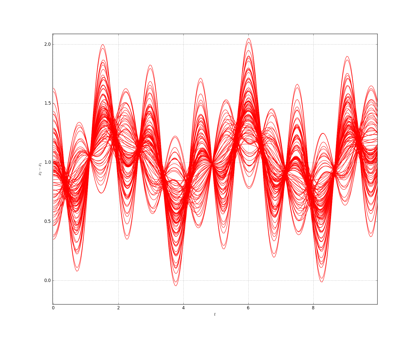
As dictated by Theorem 4, we consider an extended vector field over the variables1414 14 In practice, it is superfluous to introduce auxiliary copies of the constants . The same is true for : as the their initial values is fixed by , their auxiliary copies would be anyway eliminated from the final system (19). , then take a complete template of total degree 3 over and . We obtain , which takes about 60s, for some and , where
(A Gröbner basis of consists of 4 polynomials whose lengthy description is omitted here). One can check that, once fixed , for any instantiation of the variables and in , the dimension of the resulting variety is , implying it represents a good over-approximation the resulting system trajectory. Once and have been eliminated, the system (19) becomes
This algebraic system is proven to have no solutions: we give some details in Appendix D. Therefore, by virtue of Theorem 4, is safe.
We end the section by remarking that the verification method discussed so far easily extends to general semialgebraic sets. Indeed, let a continuous system have and as initial and unsafe set, respectively, where are basic semialgebraic sets. Then safety of is equivalent to safety of each one of the basic systems .
8 Discussion
We round off the technical development so far with a discussion on what novelties and benefits our approach actually delivers, also in relation to existing work. We shall focus on three aspects: extended systems, preconditions and polynomial invariants.
Extended systems and relational abstractions
Our use of auxiliary variables and of extended systems to handle semialgebraic safety problems in Section 7 appears to be strongly connected to relational abstractions of odes, introduced by Sankaranarayanan and Tiwari, see [36, Def.5]. Expressed in our notation, a (timeless) relational abstraction for a system of odes (with ) is a relation such that whenever then, for some time , we have ; recall that denotes the unique solution of the system from . In other words, a relational abstraction over-approximates the set of possible transitions between states, abstracting away from time. Seeing that relational abstractions are infinite-state transition systems, one can apply to them known verification techniques for such systems, such as k-induction: this is elaborated in [36]. Now, consider the statement of our Theorem 3, and specifically the invariant ideal mentioned there: the condition precisely says that is a relational abstraction — the argument showing this fact is in the proof of the theorem itself. As discussed in Section 7, can be obtained by running the post algorithm. Therefore post can also be seen as a relatively complete method for computing algebraic relational abstractions.
Direct and generic approaches to preconditions
Throughout the preceding sections, we have been emphasizing the important role played in our approach by preconditions . Summing up, there are two distinct sensible ways one can make use of this information in conjunction with the post algorithm.
- 1.
Direct approach: use directly as an argument of post, and obtain an algebraic invariant containing the precondition from .
- 2.
Generic approach: introduce new variables and to represent arbitrary initial conditions and compute a set of parametrized invariant ideals by running . Then syntactically replace by in the description of the precondition and add the resulting system of equations, representing the constraints on the initial conditions, to .
The generic approach is basically how we have handled semialgebraic problems in Section 7. It is instructive to compare the two approaches on one and the same example. Let us reconsider the 3D Lotka-Volterra system of Example 6, where we have already applied the generic approach. Let us now apply the direct approach to this system. Introducing an extra slack variable , and extending with , we can define the set of initial conditions as the algebraic variety . Running post with and a complete template of degree 3, after iterations and s we obtain . The invariant ideal is generated by the polynomial
As (Theorem 1(b)), we have , that is, the the system’s trajectories starting from never leave . To prove safety, it is then enough to check that . Ultimately, this reduces to proving that the algebraic system has no real solutions, which can be readily checked to be the case via the same SOS programming technique1515 15 Or, in this simple case, by just feeding to a computer algebra system. illustrated in Section 7. In this case, the direct approach leads to a gain in terms of execution time. This gain is mainly imputable to the smaller number of variables. Moreover, in this and other examples, starting from a specific precondition apparently leads to a faster convergence of post. However, the direct approach often fails, as the smallest algebraic invariant including is simply not precise enough (too large) to establish safety. This is the case with the spring-mass system of Example 7, as there is no nontrivial algebraic invariant including the given initial set.
The generic approach appears to be more effective at chasing invariants: informally, not just one, but a whole family of polynomial invariants can be captured at once, provided the family can be described parametrically with respect to a generic point . Note however that when the dependence from is not parametric, and invariance only holds for certain values may take on, the generic approach fails. For instance, the system has both and as polynomial invariants for : indeed e.g. . However, neither is found using the generic approach. Vice-versa, both invariants are found using the direct approach, with the precondition , the single point where the lines and intersect.
First-, second- and higher order integrals
Consider an invariant ideal , possibly found using post, and any . If , is called a Darboux polynomial. An important special case of Darboux polynomials is when , which, in the language of mathematical physics, makes a so-called first integral of the system. In our terminology, up the to an additive constant, first integrals coincide with polynomials that are invariants for each in the sense of Definition 1. A Darboux polynomial which is not a first integral is also known as a second integral in mathematical physics. Polynomials of an invariant ideal other than Darboux are collectively designated as higher order integrals; see [16, Ch.2]. Integrals of any order are important in applications, as the knowledge of any one of them decreases the number of degrees of freedom of the system — in our terminology, the dimension of the smallest algebraic variety including the system’s trajectories. Finding all polynomial first integrals, up to a given degree, can be done quite easily using just templates and linear algebra: indeed, the constraints for the derivative of the parametric template to be the zero polynomial are always linear. Things get harder when one needs to compute second integrals and beyond. post seamlessly computes polynomial integrals of any order up to a given degree. It is interesting to inspect the invariant ideals of the examples seen so far, and check how many polynomials, in the corresponding sets of generators, are computationally interesting, i.e. not first integrals. Table 1 displays how many integrals of each type have been found for each example by post. In all considered cases, but Kepler’s First Law, the set of generators is also a Gröbner basis. Appendix C presents the details of a higher order integral from the Collision Avoidance example.
| Example | # 1st integrals | # 2nd integrals | # higher order integrals |
|---|---|---|---|
| Collision Avoidance | 6 | 0 | 6 |
| Airplane Vertical Motion | 3 | 0 | 12 |
| Kepler 1st Law | 0 | 0 | 9 |
| Kepler 2nd & 3rd Laws | 0 | 1 | 1 |
| 3D Lotka-Volterra | 2 | 0 | 0 |
| Spring-mass System | 2 | 0 | 2 |
9 Conclusion, further and related work
We have provided complete algorithms to compute relativized strongest postconditions for systems of polynomial odes. These algorithms can be used to check safety assertions, to discover complete sets of polynomial invariants that fit a given template, and to compute largest algebraic varieties of initial conditions making given polynomial invariants true (weakest preconditions). Effectiveness of the algorithms has been demonstrated on nontrivial systems, including semialgebraic ones.
Our previous work [6] deals with simple initial values problems, where the precondition always consists of a singleton. This restriction prevents one from dealing with the most interesting continuous systems, such as semialgebraic systems. In particular, the concepts of weakest precondition is absent in [6]. The present paper lifts the algorithm of [6] to general (semi)algebraic systems. This requires considering a general algebraic precondition, described by a Gröbner basis , rather than a singleton. Among the new technical ingredients necessary to make this extension work the following two are crucial: (a) the property that, under suitable conditions, reduction modulo and substitution commute with each other (Lemma 3); (b) the use of auxiliary variables and generic initial conditions to circumvent the real radical problem (see e.g. Proposition 1 and Theorem 3). The method introduced in [6] has its roots in a line of research concerning weighted automata, bisimulation and Markov chains [4, 3, 5]. Also related to the present paper is [8], where we apply the notion of invariant ideal to the construction of linear abstractions of continuous systems.
The study of the safety of hybrid systems can be shown to reduce constructively to the problem of generating invariants for their differential equations [28]. Many authors have therefore focused on the effective generation of invariants of a special type. For example, Tiwari and Khanna consider invariant generation based on syzygies and Gröbner basis [42]. Sankaranarayanan [35] characterizes greatest invariants in terms of a descending chains of ideals. This iteration does not always converge, thus a relaxation in terms of bounded-degree pseudoideals is considered: the resulting algorithm always converges, because pseudoideals form basically a descending chain of finite-dimensional vector spaces, and returns an invariant ideal, although with no guarantee of maximality [35, Th.4.1]. By contrast, the convergence of our algorithm Post is essentially based on the stabilization of ascending chains of ideals, with completeness guarantees. Matringe et al. encode invariants constraints using symbolic matrices [32].
Our work is closely related to Ghorbal and Platzer’s [15], which gives a complete characterization of what it means for an algebraic set to be invariant for a polynomial ode. It is interesting to contrast the completeness statements in [15] and of that in the present paper with one another. [15] presents a method that, given a polynomial template and an integer , determines the largest subspace of template instantiations under which a length chain of Lie derivatives forms an invariant. Any invariant can be reduced to this form, for suitably large . In contrast, our Theorem 1, given a template and an algebraic variety , determines the largest subspace of the template instantiations that are polynomial invariants for trajectories starting from ; moreover, it determines, via , the largest invariant variety that includes . Neither of these two statements is stronger or more general than the other. From our point of view, taking the initial set explicitly into account, as we do, has some advantages. First, invariants returned by our method can be made explicitly dependent on initial conditions, via auxiliary variables, such as in the longitudinal airplane motion. As such, these invariants can be used directly within semialgebraic verification methods based on Positivstellensatz: as seen in Section 7, this amounts to proving the unsatisfiability of a set of polynomial (in)equations, also involving the auxiliary variables, corresponding to the initial set, to the polynomial invariants, and to the unsafe set. Second, knowing the precondition , we are in effect confining ourselves to a subset of the algebraic invariants, those that involve points in : this might explain the observed gain in efficiency — practically speaking, as the worst-case complexity is left unchanged. This gain is reflected in the execution times of [15] and of our algorithm, for the examples reported in Section 6. As a more general remark, we note that the computational ingredients of [15], such as minimization of the rank of a symbolic matrix (also employed in [32]), are quite different from ours. In the future, we would like to experimentally compare these two approaches on a more systematic basis than what we have done in the present paper.
The recent work of Kong et al. [17] considers generation of invariant clusters, again based on templates. Nonlinear constraints on template parameters are resolved via symbolic computation; safety for semialgebraic systems is reduced, via Positivstellensatz, to Sum-of-Squares (SOS) programming. In terms of effectiveness, this method appears to considerably improve previous techniques. Kong et al.’s approach has strong similarities with our method for semialgebraic systems. Rather than relying on clusters, we generate families of invariants via the introduction of auxiliary variables , denoting arbitrary points in the corresponding varieties. Differently from our approach, though, [17] does not offer completeness guarantees in our sense. In particular, the method of [17] only sometimes works with chains of ideals that stabilize after one step, that is Darboux polynomials. On the other hand, compared to theirs, our approach appears to be slower. It would be interesting to investigate if the more general invariants returned by our algorithm could be fruitfully employed in the approach of [17].
Ideas from Algebraic Geometry have been fruitfully applied also in Program Analysis. Relevant to our work is Müller-Olm and Seidl’s [22], where an algorithm to compute all polynomial invariants up to a given degree of an imperative program is provided. Similarly to what we do, they reduce the core problem to a linear algebraic one. However, since the setting in [22] is discrete rather than continuous, the techniques employed there are otherwise quite different, mainly because: (a) the construction of the ideal chain is driven by the program’s operational semantics, rather than by Lie derivatives; (b) only the polynomial invariants satisfied by all initial program states are considered, which in a continuous setting would mostly lead to the trivial strongest postcondition. A perhaps more crucial difference is that, when computing invariants, [22] regards templates essentially as polynomials in , rather than explicitly factoring out the template parameters . This can make the involved computations less efficient, as known algorithms for computing Gröbner bases have a complexity which is exponential in the number of variables.
Most of the material in this paper has been extended and revised from the conference paper [7]. With respect to [7], here we include the following additional material: proofs, the discussion on the expressive power of auxiliary variables in Section 4, the algorithmic presentation and the discussion on radical ideals in Section 5, the examples about collision avoidance and Kepler laws in Section 6, the extension to semialgebraic continuous systems in Section 7, and an extended and revised discussion of related works in Section 8 and in the present section.
Acknowledgment
The author has benefited from stimulating discussions with Khalil Ghorbal.
References
- [1] V.I. Arnold. Ordinary Differential Equations. The MIT Press, ISBN 0-262-51018-9, 1978.
- [2] M. L. Blinov, J. R. Faeder, B. Goldstein, and W. S. Hlavacek. BioNet-Gen: software for rule-based modeling of signal transduction based on the interactions of molecular domains. Bioinformatics, 20(17): 3289-3291, 2004.
- [3] F. Bonchi, M.M. Bonsangue, M. Boreale, J.J.M.M. Rutten, and A. Silva. A coalgebraic perspective on linear weighted automata. Inf. Comput. 211: 77-105, 2012.
- [4] M. Boreale. Weighted Bisimulation in Linear Algebraic Form. CONCUR 2009, LNCS 5710: 163-177, Springer, 2009.
- [5] M. Boreale. Analysis of Probabilistic Systems via Generating Functions and Padé Approximation. ICALP 2015 (2) 2015: 82-94, LNCS 9135, Springer, 2015. Extended version available as DiSIA working paper 2016/10, http://local.disia.unifi.it/wp_disia/2016/wp_disia_2016_10.pdf.
- [6] M. Boreale. Algebra, coalgebra, and minimization in polynomial differential equations. In Proc. of FoSSACS 2017, LNCS 10203:71-87, Springer, 2017. Full version in Logical Methods in Computer Science 15(1), 2019.
- [7] M. Boreale. Complete algorithms for algebraic strongest postconditions and weakest preconditions in polynomial odes. SOFSEM 2018: Theory and Practice of Computer Science - 44th International Conference on Current Trends in Theory and Practice of Computer Science, LNCS 10706:442-455, Springer, 2018.
- [8] M. Boreale. Algorithms for exact and approximate linear abstractions of polynomial continuous systems. HSCC 2018: 207-216, ACM, 2018.
- [9] B. Buchberger. Theoretical Basis for the Reduction of Polynomials to Canonical Forms. ACM SIGSAM Bulletin 10(3): 19–29. doi:10.1145/1088216.1088219. ACM, 1976.
- [10] D. Cox, J. Little, and D. O’Shea. Ideals, Varieties, and Algorithms An Introduction to Computational Algebraic Geometry and Commutative Algebra. Undergraduate Texts in Mathematics, Springer, 2007.
- [11] W. Decker, G.-M. Greuel, G. Pfister, H. Schönemann. Singular 4-1-2 — A computer algebra system for polynomial computations. http://www.singular.uni-kl.de, 2019.
- [12] M.S. El Din, Zhi-H. Yang, L. Zhi. On the Complexity of Computing Real Radicals of Polynomial Systems. ISSAC 2018: 351-358, ACM, 2018.
- [13] J.-C. Faugère. A new efficient algorithm for computing Gröbner bases. Journal of Pure and Applied Algebra 139(1): 61–88. doi:10.1016/S0022-4049(99)00005-5. ISSN 0022-4049. 1999.
- [14] J.-C. Faugère. A new efficient algorithm for computing Gröbner bases without reduction to zero. Proceedings of the 2002 International Symposium on Symbolic and Algebraic Computation (ISSAC), pp. 75–83. doi:10.1145/780506.780516. ISBN 978-1-58113-484-1. ACM, 2002.
- [15] K. Ghorbal, A. Platzer. Characterizing Algebraic Invariants by Differential Radical Invariants. TACAS 2014, LNCS 8413: 279-294, 2014. Extended version available from http://reports-archive.adm.cs.cmu.edu/anon/2013/CMU-CS-13-129.pdf.
- [16] A. Goriely. Integrability and Nonintegrability of Dynamical Systems. Advanced Series in Nonlinear Dynamics: Vol. 19. doi.org/10.1142/3846. World Scientific, 2001.
- [17] H. Kong, S. Bogomolov, Ch. Schilling, Yu Jiang, Th.A. Henzinger. Safety Verification of Nonlinear Hybrid Systems Based on Invariant Clusters. HSCC 2017:163-172, ACM, 2017.
- [18] T. Krick T, A. Logar. An algorithm for the computation of the radical of an ideal in the ring of polynomials. Applied Algebra, Algebraic Algorithms and Error-Correcting Codes. AAECC 1991, LNCS 539:195-205, Springer, 1991.
- [19] A.S. Laplagne. An algorithm for the computation of the radical of an ideal. Proceedings of the 2006 international symposium on Symbolic and algebraic computation. ISSAC 2006, pp 191-195, ACM, 2006.
- [20] J-B. Lasserre, M. Laurent, B. Mourrain, P. Rostalski, Ph. Trébuchet. Moment matrices, border bases and real radical computation. Journal of Symbolic Computation, 51:63-85, 2013.
- [21] J. Liu, N. Zhan, H. Zhao. Computing Semi-algebraic Invariants for Polynomial Dynamical Systems. EMSOFT: 97-106, ACM, 2011.
- [22] M. Müller-Olm and H. Seidl. Computing polynomial program invariants. Information Processing Letters 91(5), 233-244, 2004.
- [23] R. Neuhaus. Computation of real radicals of polynomial ideals - II. Journal of Pure and Applied Algebra 124 (1-3): 261-280, 1998.
- [24] D. Novikov and S. Yakovenko. Trajectories of polynomial vector fields and ascending chains of polynomial ideals. Annales de l’institut Fourier 49(2): 563-609, 1999.
- [25] P. Parrilo. Semidefinite programming relaxations for semialgebraic problems. Mathematical Programming 96(2): 293-320, 2003.
- [26] H. Peyrl and P.A. Parrilo. Computing sum of squares decompositions with rational coefficients. Theoretical Computer Science, 409: 269-281. Elsevier, 2008.
- [27] A. Platzer. Differential dynamic logic for hybrid systems. J. Autom. Reasoning 41(2), 143-189, 2008.
- [28] A. Platzer. Logics of dynamical systems. LICS 2012: 13-24, IEEE, 2012.
- [29] A. Platzer. The structure of differential invariants and differential cut elimination. Logical Methods in Computer Science 8(4): 1-38, 2012.
- [30] S. Prajna, A. Papachristodoulou, P. Seiler, P. Parrilo. SOSTOOLS and its control applications. Positive polynomials in control, pp. 580- 580, 2005.
- [31] G.R. Putland. A self-contained derivation of Kepler’s laws from Newton’s laws. https://www.grputland.com/2013/12/self-contained-derivation-of-keplers-laws-from-newtons-laws.html, 2013.
- [32] R. Rebiha, A. V. Moura, and N. Matringe. Generating invariants for non-linear hybrid systems. Theoretical Computer Science, 594:180-200, 2015.
- [33] SageMath, free open-source mathematics software, http://www.sagemath.org/.
- [34] S. Sankaranarayanan, H. Sipma, and Z. Manna. Non-linear loop invariant generation using Gröbner bases. POPL 2004: 318-329, ACM, 2004.
- [35] S. Sankaranarayanan. Automatic invariant generation for hybrid systems using ideal fixed points. HSCC 2010: 221-230, ACM, 2010.
- [36] S. Sankaranarayanan, A. Tiwari. Relational Abstractions for Continuous and Hybrid Systems. CAV 2011: 686-702. Springer, 2011.
- [37] Z. She, D. Song, M. Li. Safety Verification of Hybrid Systems Using Certified Multiple Lyapunov-Like Functions. Computer Algebra in Scientific Computing - 17th International Workshop, CASC 2015. LNCS 9301: 440-456. Springer, 2015.
- [38] A. Sogokon, K. Ghorbal, P.B. Jackson and A. Platzer. A method for invariant generation for polynomial continuous systems. In Verification, Model Checking, and Abstract Interpretation - 17th International Conference, VMCAI 2016, LNCS 9583:268-288. Springer, 2016.
- [39] R.F. Stengel. Flight Dynamics. Princeton University Press, 2004.
- [40] G. Stengle. A Nullstellensatz and a Positivstellensatz in Semialgebraic Geometry. Mathematische Annalen. 207(2): 87-97, 1974.
- [41] A. Tiwari. Approximate reachability for linear systems. HSCC 2003: 514-525, ACM, 2003.
- [42] A. Tiwari, G. Khanna. Nonlinear systems: Approximating reach sets. HSCC 2004:600-614, ACM, 2004.
- [43] M. Tribastone, S. Gilmore, and J. Hillston. Scalable differential analysis of process algebra models. IEEE Trans. Software Eng., 38(1):205-219, 2012.
Appendix A A simple algorithm for weakest preconditions
Fix a vector field . Let be a user specified postcondition, with a finite set of polynomials. We define inductively the sets , , as follows: and . For , we let
| (20) |
Let be the least integer such that , which must exist as forms an infinite ascending chains of ideals that must eventually stabilize. We let . Note that the termination condition reduces to checking equality between two ideals, which can be effectively done (Section 2).
Theorem A.1 (correctness and completeness of pre)
Let be an algebraic variety and . Then .
Proof Let . It is easy to check that and that is an invariant ideal. By Lemma 5 then is an algebraic invariant of , that is . Moreover, as , , hence . This shows that is a valid precondition of . We now show that it is actually the largest. Consider any such that and any . This means that, for each , is a polynomial invariant for . That is (Lemma 2), for each and , . Therefore, .
Appendix B Proofs of Section 4
Proof of Lemma 1 The function of the real variable is analytic in a neighborhood of 0. Hence it is identically 0 if and only if all of its derivatives, for , vanish at . Then (5) and (4) establish the result.
In the proof of the next lemma, we shall rely on the notion of monomial ordering [10, Ch.2,§2], which we introduce below.
Definition B.1 (monomial ordering)
Let . A monomial ordering on is a relation on such that: (i) is a total order on ; (ii) whenever and then ; (iii) is a well-ordering on : every nonempty subset of has a smallest element under .
Let be distinct indeterminates. For , let denote the monomial . The monomial order is lifted to the set of monomials over by letting iff . In , is the multidegree of , denoted . The leading term of a polynomial is the monomial appearing in of highest multidegree; then .
An example of monomial ordering is the lexicographic order: at the level of multidegrees, for and one lets if the leftmost nonzero entry of the vector difference is positive. One lets iff . For instance, for , one has .
Proof of Lemma 3 Consider the template as an element of , for . Note that, by our choice of a lexicographic order where for any , we have for example, , whatever .
Now let , where again . We first prove that is a template as well, that is, the template parameters can occur only linearly in . By the properties of multivariate division [10, Ch.2,§3,Th.3], there is a , with and , such that
| (21) |
Moreover, again by the same result: (a) ; (b) is a linear combination of monomials, none of which is divisible by the leading term of any polynomial in . Assume by contradiction there is in a summand (), where a template parameter occurs in the monomial with a degree . By the linearity of in the template parameters in and by (21), we deduce that must be a summand of (seen as a linear combination of monomials), so that the two terms can cancel each other. We deduce that . Hence, by (a) above and transitivity, . But this is impossible: indeed, by the chosen lexicographic order, we must have , because is linear in all the template parameters in , whereas in the degree of is .
Now, consider any . By (21) we have . Clearly , where is here the ideal in generated by . Moreover, (b) above implies that none of the monomials in is divisible by the leading term of any polynomial in . Since is a Gröbner basis in , these two properties say that is the (unique) remainder of the division of by : see e.g. [10, Ch.2,§6,Prop.1]. In other words, .
Proof of Lemma 4 We proceed by induction on . The base case follows from the definition of . Assuming by induction hypothesis that and that , we prove now that and that . The key to the proof is the following fact
| (22) |
From this fact the thesis will follow, indeed:
- 1.
. To see this, observe that for each (the equality here follows from the induction hypothesis), it follows from (22) that can be written as a finite sum of the form , with and . For each , by assumption, from which it easily follows that also . This shows that and proves that . The reverse inclusion is obvious;
- 2.
. As a consequence of (the previous point), we can write
where the last step follows by induction hypothesis. From (22), we have that , which implies the thesis for this case, as .
We prove now (22). Fix any . First, note that (here we are using (9)). As by induction hypothesis , we have that can be written as a finite sum , with and . Applying the rules of Lie derivatives (2), (3), we find that equals
Now, for each , , each term , with , is by definition in . This proves that , as required.
Proof of Lemma 5 First assume that is an algebraic invariant. Take . This is by definition an ideal. We show that is invariant. Indeed, take any and : by hypothesis, , hence , for each , that is is a polynomial invariant for . But, by Lemma 2, this is equivalent to for each , in particular, . Since is arbitrary, . Since is arbitrary, we have that is an invariant ideal.
Conversely, assume that for an invariant ideal. Of course is algebraic. We show that is invariant, that is that . Indeed, take any and : by hypothesis, for each , hence for each . Again by Lemma 2, this means that is identically 0. Since is arbitrary, this means that for each . Since is arbitrary, we have that is an invariant.
Concerning part (b), let , the weakest precondition (algebraic variety) for . Let . We first prove that . Indeed, one one hand, by definition of we have that and therefore: , where the first equality comes from Theorem 1(a). On the other hand, by definition of , which implies , therefore we have: , where the first equality comes again from Theorem 1(a). Thus we have proved . Now by Theorem 1(b) and , we deduce that .
Now we prove that . Since, by definition of , , we must have ; but (again Theorem 1(b)), hence we have , that is . On the other hand, by part (a), is an algebraic invariant, that is ; hence, since and , we get ; the latter implies , by definition of . In conclusion, .
Appendix C Details for the collision avoidance example of Section 6
The following is a Gröbner basis of the invariant ideal w.r.t. the lexicographic order induced by the following ordering of variables: .
Let be the first polynomial listed in above. Let us check that is not a first integral. In fact, is not even a Darboux polynomial. To see this, let us compute explicitly the Lie derivative of
It is immediate to check that with the help of a computer algebra system. This can also be checked manually, noting that is trivially a Gröbner basis of w.r.t. the lexicographic order, and that . Indeed, the leading monomial of , that is , is not divisible by the leading monomial of , that is . The least such that is .
Appendix D Proof of Theorem 4, Positivstellensatz and SOS programming in Section 7
Proof of Theorem 4 By contradiction, assume there are and , for some . We will show that is a solution of (19), thus arriving at a contradiction. Indeed, by definition and , for each and . Consider now the trajectory of originating from , that is : note that, by definition of , for each . Now, since , we have , hence, by -invariance of , for each (Lemma 5). In particular, considering , we have . But this means for . In conclusion, is a solution of (19).
When working in algebraically closed fields, like , Hilbert’s Nullstellensatz [10] implies that a system of polynomial equations has no solution if and only if . This gives a simple criterion to check if is solvable. The following result, often considered as the real algebraic counterpart of Hilbert’s Nullstellensatz, is due to Stengle [40]. Let us introduce the necessary terminology. In what follows, all polynomials are in for some fixed . A polynomial is a Sum of Squares (SOS) if , for some polynomials . Given a finite set of polynomials , the cone generated by is .
Theorem D.1 (Positivstellensatz)
Let and be two sets of polynomials. The system of (in)equations has no solution in if and only if there are and such that .
If one writes as and as , then finding and such that can be formulated as follows:
| (23) |
Now a polynomial is SOS if and only if there is a vector of monomials and a real symmetric positive semidefinite matrix such that . Once bases of monomials have been fixed for each of the (unknown) polynomials and , one can consider a relaxation of problem (23), whereby one searches for polynomials built from those bases satisfying (23) (empty bases are allowed). Problem (23) becomes in this way a semidefinite programming problem [25], with one variable for each (unknown) polynomial coefficient, and constraints given by the various positive semidefinite conditions and by the equation (23). In fact, there are tools, like SOSTOOLS [30], to efficiently convert relaxations of problem (23) into a semidefinite programming problem and then try to solve it via numerical techniques. If successful, the obtained SOS polynomial is a certificate of insolvability of the original system. Although the number of terms in (23) is potentially exponential in , experience has shown that, in practice, this technique tends to yield short (low degree) certificates, if the original system is actually not solvable.
For the continuous semialgebraic systems in Examples 6 and 7, denoting by the polynomials defining and in each case, problem (23) takes the following concrete form
| (24) |
For Example 6, fixing a maximum degree of for the ’s and of for the ’s and running SOSTOOLS under Matlab1616 16 Matlab scripts for both examples are available at https://github.com/micheleatunifi/postconditions/blob/master/SOSSafety.m. we solve (24), finding the following polynomials, which yield a low-degree certificate:
This takes about 0.4s on a Core i5 machine under Windows 10. A certificate for Example 7 is found in a similar way; we omit here the lengthy description of the corresponding polynomials.
Remark D.1 (dealing with roundoff errors)
It is important to ensure that the SOS decomposition found numerically actually corresponds to a true solution, and it is not the result of roundoff errors that may arise when working in floating point arithmetic. There are several ways of doing this: for instance, by computing exact rational solutions, that can be fully verified symbolically, or by tweaking the numerical coefficients of a candidate solution; see for instance [26, 37]. In particular, the SOSTOOLS findSOS procedure incorporates an experimental ’rational’ option, that will try to produce an exact rational SOS representation of the input polynomial. Using this option, we have checked that the solution found for the Lotka-Volterra example is indeed SOS. On the other hand, the ’rational’ option fails to find a rational representation in the spring-mass example.