Proca stars with nonminimal coupling to the Einstein tensor

In this section, we discuss PSs in the theory (1). We consider a static and spherically symmetric spacetime

where $\hat{t}$ and $r$ are the time and radial coordinates, $d\Omega_{2}^{2}$ is the metric of the unit two sphere, and $m(r)$ and $\sigma(r)$ depend only on the radial coordinate $r$. Correspondingly, we consider the ansatz for the vector field [33]

where $a_{0}(r)$ and $a_{1}(r)$ depend only on $r$. We assume that the frequency ${\hat{\omega}}$ is real, ensuring that the vector field neither grows nor decays. Equation (9) avoids the restrictions from Derrick’s theorem that forbid stable localized solutions to nonlinear wave equations [37]. The explicit time dependence $e^{-i{\hat{\omega}}{\hat{t}}}$ does not induce the time dependence in the metric. In order to find $m(r)$, $\sigma(r)$, $a_{0}(r)$, and $a_{1}(r)$, we solve the evolution equation derived from EOMs (2), (5), and (6).

From our ansatz (8) and (9), the $({\hat{t}},{\hat{t}})$, $(r,r)$ and angular components of the gravitational EOM (2)

are given by Eq. (23) with Eq. (24). Similarly, the $t$ and $r$ components of the vector field EOM (5),

are given by Eq. (25) with Eq. (26). Finally, Eq. (6) is given by Eq. (27) with Eq. (28). These equations are constrained by the identity

Combining them, we obtain a set of the evolution equations (29a), (29b), (29c), and (33) which determine the structure of PSs from the center $r=0$ to spatial infinity $r=\infty$.

Solving EOMs near the center $r=0$, we obtain the boundary conditions

With Eq. (13), we numerically integrate Eqs. (29a), (29b), (29c), and (33) toward the spatial infinity $r=\infty$. From Eq. (13), for $f_{0}=0$ we obtain $\sigma(r)=\sigma_{0}$ and $m(r)=a_{0}(r)=a_{1}(r)=0$, namely the Minkowski solution.

For a correct eigenvalue of ${\hat{\omega}}$, we find the asymptotically flat solution where $m(r)$ and $\sigma(r)$ exponentially approach constant values, $m_{\infty}>0$ and $\sigma_{\infty}>0$, respectively, while $a_{0}(r)$ and $a_{1}(r)$ exponentially approach zero as $e^{-\sqrt{\mu^{2}-{\hat{\omega}}^{2}/\sigma_{\infty}^{2}}r}$. Thus, in the large $r$ limit the metric exponentially approaches the Schwarzschild form

where the proper time measured at $r=\infty$ is given by $t=\sigma_{\infty}{\hat{t}}$, and correspondingly the proper frequency $\omega$ is given by

The exponential fall-off condition $e^{-\sqrt{\mu^{2}-\omega^{2}}r}$ requires $\omega<\mu$. We numerically confirmed that in the limit $f_{0}\to 0$, namely in the limit of the Minkowski solution, $\omega\to\mu$, leaving no $r$ dependence in the large $r$ limit.

Having numerical solutions, we then evaluate the conserved quantities which characterize PSs. The first is associated with the time translational symmetry and corresponds to the ADM mass

The second is the Noether charge associated with the global $U(1)$ symmetry, which is given by integrating $j^{\hat{t}}$ in Eq. (7) over a constant time hypersurface

As for a BS, a PS is said to be gravitationally bound if

As for BSs mentioned in Sec. I, for PSs we use Eq. (18) as a necessary condition for stability.

We then define the effective radius [24]

and the (effective) compactness

In contrast to the cases of BHs and NSs, for PSs $r={\cal R}$ is not the surface of $A_{\mu}=0$. Nevertheless, due to the exponential falloff property of $A_{\mu}$, ${\cal R}$ represents the characteristic length scale of energy localization. The parameter ${\cal C}$ is very important to distinguish various compact objects in different theories in light of future GW observations.

For numerical analyses, we may fix some parameters to unity. First, by rescaling

we can rewrite Eqs. (29a), (29b), (29c), and (33) into equations without $\mu$ and $\kappa$. Hence, we may work by setting $\mu=\kappa=1$. Moreover, as $\sigma_{0}$ corresponds to the time rescaling at the center $r=0$, we may also set $\sigma_{0}=1$ for convenience. In general, then $\sigma_{\infty}\neq 1$ and quantities measured at the spatial infinity can be obtained by performing the rescalings discussed in Sec. III.3. Thus, the only remaining parameters are $f_{0}$ and $\beta$. For a fixed value of $\beta$, by varying $f_{0}$ we numerically integrate them and evaluate the above quantities. In Fig. 1, by setting $\mu=\kappa=\sigma_{0}=1$, $m(r)$, $\sigma(r)$, $a_{0}(r)$, and $a_{1}(r)$ are shown as functions of $r$ for $\beta=0.2$ and $f_{0}=1.0$, which are very similar to the case of $\beta=0$ [33, 34].

Before proceeding, we briefly comment on the massless case $\mu=0$. In this case, by rescaling

the dependence on ${\hat{\omega}}$ is completely eliminated from EOMs. Thus, the problem does not reduce to the eigenvalue one. As $\beta$ is dimensionless, for $\mu=0$ there is no physical scale which characterizes PSs. Thus, there is no PS solution only by nonminimal coupling.

In Fig. 2, for $\beta=0.2$, $0.1$, $0$, $-0.1$, and $-0.2$, $\omega/\mu$ is shown as a function of $f_{0}$. In all cases, for $f_{0}\to 0$, $\omega/\mu\to 1$ which reproduces the Minkowski solution.

For $\beta=0$, there are several branches of PSs for a single value of $\omega$. As $f_{0}$ increases from zero, $\omega/\mu$ decreases from $1$ and reaches the minimal value $0.814$ for $f_{0}\approx 0.199M_{p}$. Then, $\omega/\mu$ increases and reaches the local maximal value $0.906$ for $f_{0}\approx 2.39M_{p}$. As $f_{0}$ increases further, $\omega/\mu$ gradually approaches $0.891$. For nonzero values of $\beta$, irrespective of its sign, numerical PS solutions cease to exist for $f_{0}$ above some certain value. However, the reasons are different for $\beta>0$ and $\beta<0$.

For $\beta>0$, there are several branches of PSs for a single value of $\omega$. However, for $f_{0}$ above some certain value depending on $\beta$, $\tilde{\cal C}_{1}$ in Eq. (33) always vanishes at a very small radius, and no PS solutions exist. In our examples, no PS solutions are found for $f_{0}\gtrsim 0.349M_{p}$ for $\beta=0.1$ and for $f_{0}\gtrsim 0.231M_{p}$ for $\beta=0.2$. Before reaching these values of $f_{0}$, $\omega/\mu$ takes the minimal values $0.827$ for $f_{0}\approx 0.160M_{p}$ ($\beta=0.1$) and $0.836$ for $f_{0}\approx 0.140M_{p}$ ($\beta=0.2$). Thus, for larger nonminimal coupling parameters, PS solutions cease to exist for smaller amplitudes.

For $\beta<0$, $\omega/\mu$ always decreases. Although $\tilde{\cal C}_{1}$ in Eq. (33) does not vanish at any radius, it becomes extremely small for larger values of $f_{0}$, making numerical integrations unstable unless sufficiently high resolutions are taken. Thus, although we will show PS solutions only for smaller values of $f_{0}$ where numerical integration can be performed stably, in principle it does not forbid the existence of PS solutions for larger values of $f_{0}$. In our analysis, numerical integration could not performed stably for $f_{0}\lesssim 0.628M_{p}$ for $\beta=-0.1$ and for $f_{0}\lesssim 0.409M_{p}$ for $\beta=-0.2$.

In Figs. 3-5, for $\beta=0$, $0.2$, and $-0.2$, $M$ and $\mu Q$ are shown as functions of $\omega/\mu$. For all cases, $f_{0}=0$ gives the Minkowski solution $M=Q=0$ with $\omega=\mu$. Moreover, even in the presence of the nonminimal coupling to the Einstein tensor PS solutions obtained in our analysis are mini-BS type, where $M$ and $\mu Q$ are typically $\sim M_{p}^{2}/\mu$.

The case of $\beta=0$ is shown in Fig. 3. As $f_{0}$ increases from zero, $M$ and $\mu Q$ increase from zero while $\omega/\mu$ decreases from $1$. $M$ and $Q$ then take their maximal values, $M_{\rm max}\approx 1.06M_{p}^{2}/\mu$ and $\mu Q_{\rm max}\approx 1.09M_{p}^{2}/\mu$ for $\omega/\mu\approx 0.870$, which satisfies Eq. (18) and agrees with Ref. [33]. Then $\omega/\mu$ still decreases, while $M$ and $\mu Q$ start to decrease. After $\omega/\mu$ reaches its minimal value $0.814$, it starts to increase while $M$ and $\mu Q$ still decrease until reaching their local minimum values, $M_{\rm min}\approx 0.496M_{p}^{2}/\mu$ and $\mu Q_{\rm min}\approx 0.412M_{p}^{2}/\mu$, respectively. In this region, Eq. (18) is not satisfied. As $f_{0}$ increases further, $M$ and $\mu Q$ eventually converge to $M\approx 0.563M_{p}^{2}/\mu$ and $\mu Q\approx 0.486M_{p}^{2}/\mu$, respectively.

The case of $\beta=0.2$ is shown in Fig. 4. As $f_{0}$ increases from zero, $M$ and $\mu Q$ increase from zero while $\omega/\mu$ decreases from $1$. $M$ and $\mu Q$ then take their maximal values, $M_{\rm max}\approx 1.05M_{p}^{2}/\mu$ and $\mu Q_{\rm max}\approx 1.07M_{p}^{2}/\mu$, for $\omega/\mu\approx 0.872$, which satisfies Eq. (18). Then as $\omega/\mu$ still decreases, $M$ and $\mu Q$ start to decrease. After $\omega/\mu$ reaches its minimal value $0.836$, $\omega/\mu$ starts to increase while $M$ and $\mu Q$ still decrease. In this region, Eq. (18) is not satisfied. As we discussed in Sec. IV.1, for $\beta=0.2$, we can obtain PS solutions up to $f_{0}=0.231M_{p}$, for which $M\approx 0.768M_{p}^{2}/\mu$ and $\mu Q\approx 0.744M_{p}^{2}/\mu$.

Finally, the case of $\beta=-0.2$ is shown in Fig. 5. As $f_{0}$ increases from zero, $M$ and $\mu Q$ increase from zero while $\omega/\mu$ decreases from $1$. $M$ and $\mu Q$ then take their maximal values, $M_{\rm max}\simeq 1.07M_{p}^{2}/\mu$ and $\mu Q_{\rm max}\simeq 1.10M_{p}^{2}/\mu$ for $\omega/\mu\approx 0.868$, which satisfies Eq. (18). As $f_{0}$ increases further, $M$ and $\mu Q$ decrease while $\omega$ still decreases. As we discussed in Sec. IV.1, for $\beta=-0.2$, for $f_{0}$ above $0.409M_{p}$, we could not find numerical PS solutions due to the problem discussed in Sec. IV.1. For $f_{0}=0.409M_{p}$, $M\approx 0.727M_{p}^{2}/\mu$ and $\mu Q\approx 0.667M_{p}^{2}/\mu$. For $\omega/\mu\lesssim 0.792$, Eq. (18) is not satisfied.

In Fig. 6, $M$ (the left panel) and $\mu Q$ (the right panel) are shown for all $\beta=0.2$, $0.1$, $0$, $-0.1$, and $-0.2$. $M$ and $\mu Q$ almost coincide for larger $\omega/\mu$, i.e., smaller $f_{0}$. As $M$ and $\mu Q$ approach their maximal values, $\beta$ dependence becomes more evident, and for negative (positive) values of $\beta$, both $M$ and $\mu Q$ take larger (smaller) values than those for $\beta=0$ for the same $\omega$. Moreover, for both positive and negative values of $\beta$, spiraling features observed for $\beta=0$ eventually disappear. Such behaviors are very similar to those observed for BSs in the EGB theory [30, 31], the EdGB theory [32] and the complex scalar-tensor theory with nonminimal derivative coupling to the Einstein tensor [29]. Thus, they may be generic for healthy higher-derivative theories.

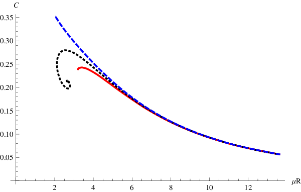
In Fig. 7, for $\beta=0.2$, $0.1$, $0$, $-0.1$, and $-0.2$, $M$ is shown as a function of $\mu{\cal R}$ defined in Eq. (19). In all cases, for larger $f_{0}$, ${\cal R}$ becomes smaller, which means that energy is localized more efficiently around the center. For $\mu{\cal R}\gtrsim 6.0$, no clear $\beta$ dependence is observed, while for $\mu{\cal R}\lesssim 6.0$, $\beta$ dependence becomes more evident and a larger (smaller) value of $M$ is observed for $\beta<0$ ($\beta>0$). For $\beta=0$, $M$ is a multivalued function of ${\cal R}$, while for $\beta\neq 0$, it is a single-valued function of ${\cal R}$. Very similar behaviors are observed also for $\mu Q$ as a function of $\mu{\cal R}$. As a reference, we also show the case of ${\cal R}=2m_{\infty}$, although ${\cal R}$ has nothing to do with the Schwarzschild radius of a BH.

In Figs. 8-10, for $\beta=0$, $0.2$, and $-0.2$, $M$ and $\mu Q$ are shown as functions of $\mu{\cal R}$, respectively. For all $\beta=0$, $0.2$, and $-0.2$, for $\mu{\cal R}\gtrsim 3.5$, Eq. (18) is satisfied, while for $\mu{\cal R}\lesssim 3.5$, it is not satisfied.

In Fig. 11, for $\beta=0.2$, $0$, and $-0.2$, ${\cal C}$ as defined in Eq. (20) is shown as the function of $\mu{\cal R}$. For $\mu{\cal R}\gtrsim 6.0$, ${\cal C}$ becomes smaller and no clear $\beta$ dependence is observed, while for $\mu{\cal R}\lesssim 6.0$, $\beta$ dependence becomes more evident and a larger (smaller) value of ${\cal C}$ is observed for $\beta<0$ ($\beta>0$). For $\beta=0$, $\cal C$ is a multivalued function of ${\cal R}$, while for $\beta\neq 0$, it is a single-valued function of ${\cal R}$.

For $\beta=0$, as $f_{0}$ increases, ${\cal R}$ decreases, and ${\cal C}$ increases and takes the maximal value $0.280$ for $\mu{\cal R}\approx 2.50$. After reaching the maximal value, ${\cal C}$ starts to decrease, while $\mu{\cal R}$ still decreases and reaches the minimal value $2.12$. As $f_{0}$ further increases, ${\cal C}$ eventually converges to $0.213$.

For $\beta=0.2$, as $f_{0}$ increases while $\mu{\cal R}$ decreases, ${\cal C}$ increases, takes the maximal value $0.243$ for $\mu{\cal R}\approx 3.44$, and then decreases until $\mu{\cal R}$ reaches the minimal value $3.21$.

For $\beta=-0.2$, as $f_{0}$ increases while $\mu{\cal R}$ decreases ${\cal C}$ monotonically increases and takes the maximal value $0.350$ when $\mu{\cal R}$ reaches the minimal value $2.08$ due to the technical problelm discussed in Sec. IV.1. There may be PS solutions for $\mu{\cal R}\lesssim 2.08$, for which ${\cal C}$ may be larger values than $0.350$. However, the condition (18) is not satisfied for such solutions.

Although in the given subclass of the generalized complex Proca theory the explicit analysis of stability will be quite involved, in this subsection we will give the speculation about stability in terms of the insensitivity of the critical central amplitude of the vector field $f_{0,c}$, for which PSs take the maximal values of the ADM mass $M$ and the Noether charge $Q$, to the choice of the nonminimal coupling parameter $\beta$.

We have confirmed that the value of the critical central amplitude, which in our analysis is found to be $f_{0,c}\approx 0.0399M_{p}$, is insensitive to the choice of $\beta$, although the absolute maximal values of $M$ and $\mu Q$ both depend on $\beta$. As we have mentioned in Sec. I, in the case of $\beta=0$ the PS solution with the maximal values of $M$ and $\mu Q$ corresponds to the critical solution which divides stable and unstable PS solutions [33], as in the case of BSs in the scalar-tensor theory [27, 28]. Thus, the insensitivity of the value of $f_{0,c}$ to the choice of $\beta$ indicates that even in the presence of nonminimal coupling $\beta\neq 0$ the PS solution with the maximal values of $M$ and $\mu Q$ obtained for $f_{0,c}\approx 0.0399M_{p}$ would also correspond to the critical PS solution which divides stable and unstable PS ones, and PS solutions for $f_{0}<f_{0,c}\approx 0.0399M_{p}$ would be stable, irrespective of the choice of $\beta$. The explicit confirmation of this speculation is definitively important, but will be left for future studies.

References

- [1] Timothy Clifton, Pedro G. Ferreira, Antonio Padilla, and Constantinos Skordis, “Modified Gravity and Cosmology,” Phys.Rept. 513, 1–189 (2012), arXiv:1106.2476 [astro-ph.CO] .
- [2] Emanuele Berti et al., “Testing General Relativity with Present and Future Astrophysical Observations,” Class. Quant. Grav. 32, 243001 (2015), arXiv:1501.07274 [gr-qc] .
- [3] Gregory Walter Horndeski, “Second-order scalar-tensor field equations in a four-dimensional space,” Int.J.Theor.Phys. 10, 363–384 (1974).
- [4] C. Deffayet, S. Deser, and G. Esposito-Farèse, “Generalized Galileons: All scalar models whose curved background extensions maintain second-order field equations and stress-tensors,” Phys. Rev. D80, 064015 (2009), arXiv:0906.1967 [gr-qc] .
- [5] C. Deffayet, Xian Gao, D.A. Steer, and G. Zahariade, “From k-essence to generalised Galileons,” Phys.Rev. D84, 064039 (2011), arXiv:1103.3260 [hep-th] .
- [6] Tsutomu Kobayashi, Masahide Yamaguchi, and Jun’ichi Yokoyama, “Generalized G-inflation: Inflation with the most general second-order field equations,” Prog. Theor. Phys. 126, 511–529 (2011), arXiv:1105.5723 [hep-th] .
- [7] Gianmassimo Tasinato, “Cosmic Acceleration from Abelian Symmetry Breaking,” JHEP 04, 067 (2014), arXiv:1402.6450 [hep-th] .
- [8] Lavinia Heisenberg, “Generalization of the Proca Action,” JCAP 1405, 015 (2014), arXiv:1402.7026 [hep-th] .
- [9] Erwan Allys, Patrick Peter, and Yeinzon Rodriguez, “Generalized Proca action for an Abelian vector field,” JCAP 1602, 004 (2016), arXiv:1511.03101 [hep-th] .
- [10] Jose Beltran Jimenez and Lavinia Heisenberg, “Derivative self-interactions for a massive vector field,” Phys. Lett. B757, 405–411 (2016), arXiv:1602.03410 [hep-th] .
- [11] Antonio De Felice, Lavinia Heisenberg, Ryotaro Kase, Shinji Tsujikawa, Ying-li Zhang, and Gong-Bo Zhao, “Screening fifth forces in generalized Proca theories,” Phys. Rev. D93, 104016 (2016a), arXiv:1602.00371 [gr-qc] .
- [12] Antonio De Felice, Lavinia Heisenberg, Ryotaro Kase, Shinji Mukohyama, Shinji Tsujikawa, and Ying-li Zhang, “Cosmology in generalized Proca theories,” JCAP 1606, 048 (2016b), arXiv:1603.05806 [gr-qc] .
- [13] Antonio De Felice, Lavinia Heisenberg, Ryotaro Kase, Shinji Mukohyama, Shinji Tsujikawa, and Ying-li Zhang, “Effective gravitational couplings for cosmological perturbations in generalized Proca theories,” Phys. Rev. D94, 044024 (2016c), arXiv:1605.05066 [gr-qc] .
- [14] Javier Chagoya, Gustavo Niz, and Gianmassimo Tasinato, “Black Holes and Abelian Symmetry Breaking,” Class. Quant. Grav. 33, 175007 (2016), arXiv:1602.08697 [hep-th] .
- [15] Masato Minamitsuji, “Solutions in the generalized Proca theory with the nonminimal coupling to the Einstein tensor,” Phys. Rev. D94, 084039 (2016), arXiv:1607.06278 [gr-qc] .
- [16] Wei-Jian Geng and H. Lu, “Einstein-Vector Gravity, Emerging Gauge Symmetry and de Sitter Bounce,” Phys. Rev. D93, 044035 (2016), arXiv:1511.03681 [hep-th] .
- [17] Javier Chagoya, Gustavo Niz, and Gianmassimo Tasinato, “Black Holes and Neutron Stars in Vector Galileons,” (2017), arXiv:1703.09555 [gr-qc] .
- [18] Eugeny Babichev, Christos Charmousis, and Mokhtar Hassaine, “Black holes and solitons in an extended Proca theory,” JHEP 05, 114 (2017), arXiv:1703.07676 [gr-qc] .
- [19] Lavinia Heisenberg, Ryotaro Kase, Masato Minamitsuji, and Shinji Tsujikawa, “Hairy black-hole solutions in generalized Proca theories,” (2017), arXiv:1705.09662 [gr-qc] .
- [20] David J. Kaup, “Klein-Gordon Geon,” Phys. Rev. 172, 1331–1342 (1968).
- [21] Remo Ruffini and Silvano Bonazzola, “Systems of selfgravitating particles in general relativity and the concept of an equation of state,” Phys. Rev. 187, 1767–1783 (1969).
- [22] R. Friedberg, T. D. Lee, and Y. Pang, “MINI - SOLITON STARS,” Phys. Rev. D35, 3640 (1987), [,55(1986)].
- [23] Philippe Jetzer, “Boson stars,” Phys. Rept. 220, 163–227 (1992).
- [24] F.E. Schunck and E.W. Mielke, “General relativistic boson stars,” Class.Quant.Grav. 20, R301–R356 (2003), arXiv:0801.0307 [astro-ph] .
- [25] Marcelo Gleiser, “Stability of Boson Stars,” Phys. Rev. D38, 2376 (1988), [Erratum: Phys. Rev.D39,no.4,1257(1989)].
- [26] T. D. Lee and Yang Pang, “Stability of Mini - Boson Stars,” Nucl. Phys. B315, 477 (1989), [,129(1988)].
- [27] Marcelo Gleiser and Richard Watkins, “Gravitational Stability of Scalar Matter,” Nucl. Phys. B319, 733–746 (1989).
- [28] Scott H. Hawley and Matthew W. Choptuik, “Boson stars driven to the brink of black hole formation,” Phys. Rev. D62, 104024 (2000), arXiv:gr-qc/0007039 [gr-qc] .
- [29] Yves Brihaye, Adolfo Cisterna, and Cristian Erices, “Boson stars in biscalar extensions of Horndeski gravity,” Phys. Rev. D93, 124057 (2016), arXiv:1604.02121 [hep-th] .
- [30] Betti Hartmann, Jurgen Riedel, and Raluca Suciu, “Gauss-Bonnet boson stars,” Phys. Lett. B726, 906–912 (2013), arXiv:1308.3391 [gr-qc] .
- [31] Yves Brihaye and Jurgen Riedel, “Rotating boson stars in five-dimensional Einstein-Gauss-Bonnet gravity,” Phys. Rev. D89, 104060 (2014), arXiv:1310.7223 [gr-qc] .
- [32] Vishal Baibhav and Debaprasad Maity, “Boson Stars in Higher Derivative Gravity,” Phys. Rev. D95, 024027 (2017), arXiv:1609.07225 [gr-qc] .
- [33] Richard Brito, Vitor Cardoso, Carlos A. R. Herdeiro, and Eugen Radu, “Proca stars: Gravitating Bose-Einstein condensates of massive spin 1 particles,” Phys. Lett. B752, 291–295 (2016), arXiv:1508.05395 [gr-qc] .
- [34] Ignacio Salazar Landea and Federico Garcia, “Charged Proca Stars,” Phys. Rev. D94, 104006 (2016), arXiv:1608.00011 [hep-th] .
- [35] Y. Brihaye, Th. Delplace, and Y. Verbin, “Proca Q Balls and their Coupling to Gravity,” (2017), arXiv:1704.01648 [gr-qc] .
- [36] Richard P. Woodard, “Ostrogradsky’s theorem on Hamiltonian instability,” Scholarpedia 10, 32243 (2015), arXiv:1506.02210 [hep-th] .
- [37] G. H. Derrick, “Comments on nonlinear wave equations as models for elementary particles,” J. Math. Phys. 5, 1252–1254 (1964).