Regression estimator for the tail index
Abstract
Estimating the tail index parameter is one of the primal objectives in extreme value theory. For heavy-tailed distributions the Hill estimator is the most popular way to estimate the tail index parameter. Improving the Hill estimator was aimed by recent works with different methods, for example by using bootstrap, or Kolmogorov-Smirnov metric. These methods are asymptotically consistent, but for tail index and smaller sample sizes the estimation fails to approach the theoretical value
for realistic sample sizes. In this paper, we introduce a new empirical method, which can estimate
high tail index parameters well
and might also be useful for relatively small sample sizes.
MSC code: 62G32, 62F40, 60G70.
keywords
Tail index; bootstrap; Hill estimation; Kolmogorov-Smirnov distance
1 Introduction
In probability theory and statistics there are many applications, where it is essential to know the high quantiles of a distribution, for example solvency margin calculations for insurances or estimating the highest possible loss caused by a natural disaster within a given time period. Extreme value theory provides tools to solve these types of problems. In the 1920’s Fisher and Tippet (1928) described the limit behaviour of the maximum of i.i.d. samples. Their theorem is the basis of every research in extreme value theory. Later another approach emerged, where the extremal model is based on the values over a high threshold. Its theoretical background was developed by Balkema and de Haan (1974) and Pickands (1975), the statistical applications by Davison and Smith (1990), among others – summarized by Leadbetter (1991). Both approaches depend on the tail behaviour of the underlying distribution, which can be measured by the tail index. Hill (1975) constructed an estimator for the tail index, using the largest values of the ordered sample. This estimator is still popular, however finding the optimal number of sample elements to be used remains a challenge. Numerous methods were developed to find the best threshold, for example the double bootstrap method by Danielsson et al. (2001), improved by Qi (2008) or a model based on Kolmogorov-Smirnov distance by Danielsson et al. (2016). The Hill estimator is asymptotically consistent for both threshold selection methods, however simulations show that for some sample distributions we need more than observations for a reasonably accurate estimation. Our new method skips the direct threshold selection for the initial sample and calculates the tail index estimation via the tail indices of simulated subsamples. In this way it results in acceptable estimators for smaller samples, like too.
1.1 Mathematical overview
Let be an independent and identically distributed (i.i.d) sample from a distribution function , and . If there exist sequences and , such that
if for a nondegenerate distribution function , then one can say that is in the maximum domain of attraction of . The Fisher-Tippet theorem claims that belongs to a parametric family (with location, scale and shape parameter) called generalized extreme value distribution. For every distribution exist and , such that for every , where is the standardized extreme value distribution:
| (1) |
where holds. The parameter is called the tail index of the distribution. In case of a generalized extreme value distribution the tail index parameter is the shape parameter, which is invariant of standardizing the distribution.
Another approach to the investigation of the tail behaviour is the peaks over threshold (POT) model of Balkema and de Haan (1974) and Pickands (1975) where the extremal model is based on the values over a threshold . Let be the right endpoint of the distribution (finite or infinite). If the distribution of the standardized excesses over the threshold has a limit, that must be the generalized Pareto distribution:
where
| (2) |
For the given initial distribution , the two model result in the same parameter in equations (1) and (2).
A function is called slowly varying if for all . For tail index parameter the previous limit theorems are true if
Finding a proper function and calculating the parameters of the limiting distribution is only applicable for special known distributions. In case of real life problems finding is unrealistic, therefore one can use estimators to approximate .
2 Methods for defining the threshold in Hill estimator
For tail index Hill (1975) proposed an estimator as follows: let be a sample from a distribution function and the ordered statistic. The Hill estimator for the tail index is
Similarly to the POT model, the Hill estimator also uses the largest values of the sample. The threshold is defined as the highest observation.
The Hill estimator strongly depends on the choice for . It is important to mention that is a consistent estimator for the tail index only if as . If one uses a too small , the estimator has large variance, however for too large , the estimator is likely to be biased. Therefore proposing a method for choosing the optimal for the Hill estimator has been in the focus of research by Hall (1982) and others since its invention .
2.1 Double bootstrap
One of the most accurate estimators, the double bootstrap method was introduced by Danielsson et al. (2001), improved by Qi (2008). In this case, we can find a proposed by minimizing the asymptotic mean square error. Let
One can see, that is the Hill estimation. Instead of , the method optimizes for the mean square error of . Let be the optimal threshold index for , and for . The
| (3) |
statement is proven by Danielsson et al. (2001), where is a regularity parameter, which can be estimated in a consistent way. This statement allows to estimate instead of by following the next steps.
- •
Choose and set to ensure consistency if . Estimate by drawing size bootstrap samples from the empirical distribution function and minimize it in . Denote the minimum by .
- •
Set and minimize the same way as in the first step, let the minimum be .
- •
Estimate the regularity parameter , which is important for further calculations, by .
- •
Now one can estimate the optimal using the approximation (3) by
The Hill estimator based on the double bootstrap method provides appropriate tail index estimation, but usually results in a long computation time. For smaller sample sizes the acceptable range is limited to .
2.2 Kolmogorov-Smirnov distance metric
Another approach is to minimize the distance between the tail of the empirical distribution function and the fitted Pareto distribution with the estimated tail index parameter. One can use the Kolmogorov-Smirnov distance for the quantiles as metric as proposed by Danielsson et al. (2016). Assume that
The quantile function can be approximated by
The probability can be replaced by , and is estimated by the Hill estimator for some , moreover can be estimated by . Using these substitutions one gets an estimation for the quantiles as a function of and .
The optimal for the Hill estimator is chosen as the , which minimizes the distance between the empirical and the calculated quantiles
where sets the fitting threshold (we call it KS threshold). The advantages of this method are that it is easy to program and its computation time is short. As Danielsson et al. (2016) mentioned, it is the best performing known method if and also works well for small sample sizes. However, for distributions with tail index this technique results in highly biased estimation.
Generally it can be said, that there are good methods for finding an appropriate if the tail index parameter is , which contains distributions with finite variance. However, these methods usually fail to perform well for the case (these are distributions with infinite variance).
The Kolmogorov-Smirnov method was introduced and analized by simulations in Danielsson et al. (2016), but no theoretical background is available for this method. The Theorem 2.2 states that under some conditions the Kolmogorov-Smirnov technique results in unbiased estimation for the tail index. For the proof we need the following lemma:
Lemma 2.1.
If , then .
Proof.
For by using the Stirling formula we have
∎
Theorem 2.2.
The Hill estimatior results in asymptotically unbiased estimation for the tail index using the Kolmogorov-Smirnov -selection technique as .
Proof.
Let be our sample, and be the ordered sample. Let
| (4) |
be our unbiased quantile estimator for , similar as one can see Danielsson et al. (2016). For the right , sequences the distribution will be identical to a Pareto distribution (POT model). Therefore Glivenko-Cantelli type theorems for quantiles provides that the estimator is consistent, for every there is an such that if then the Kolmogorov-Smirnov distance will be less than .
Choose which minimizes the Kolmogorov-Smirnov distance of estimator and samples and let be the Hill estimation using if .
∎
However is not an evident condition and even if it is realized we cannot say anything about the speed of convergence. This could lead to biased tail index estimation using Kolmogorov-Smirnov method, especially if has high value.
3 Estimator for heavy-tailed distributions
The method based on Kolmogorov-Smirnov metric is asymptotically unbiased. According to Danielsson et al. (2016) the method provides acceptable results for small sample sizes if , but for tail index usually samples of more than elements are necessary to estimate properly. However, in most real-life applications such a large sample size is not available, therefore in cases of distributions with infinite variance the Kolmogorov-Smirnov metric-based estimator has significant bias.
Independent data in size from distributions with different tail index parameter were simulated to detect the magnitude of the bias. The estimations were calculated times for each . This experiment showed that the distribution of the estimator is not normal, but in spite of the different initial distributions for each , we received similar empirical distributions for the estimators, which could be approximated by a generalized extreme value distribution, as one can see in Figure 1. Although the GEV fitting is the best among known distributions, the goodness of fit tests still reject it. Therefore it would be beneficial characterizing the bootstrap distribution more precisely. We estimated the parameters of the GEV distribution using maximum likelihood method, which is a consistent estimator, although sometimes requires high sample size for proper estimation.
However, based on the simulations, one can detect a linear relation between the parameters of the best fitting GEV distribution and the theoretical tail index parameter in the interval (see Figure 2). For the mean of the estimations using the Kolmogorov-Smirnov method was acceptable. For higher index values a linear transformation can be used on the parameters of the fitted GEV distribution to estimate the tail index. When the Kolmogorov-Smirnov method could not return reasonable results, so the correction could not help.
Alternatively, the average of estimations and the theoretical tail index parameter are also in linear connection according to simulations.
After recalculating the mean values and GEV parameters for sample sizes of , and with , and simulations we experienced that the values were similar as one can see in Table 1. Due to the long calculation time no simulations were run for higher sample sizes, especially that the asymptotic behaviour of other methods are already realized for these sample sizes. With these experiments we can state that in the distribution of the Kolmogorov-Smirnov estimation does not depend on the sample size if . Deviation were detected only on , case. These results allow to use linear regression between the estimated GEV parameters and the theoretical tail index parameter.
| mean | location | scale | shape | ||
|---|---|---|---|---|---|
| , | n=500 | 0.448 | 0.378 | 0.113 | 0.043 |
| n=2000 | 0.446 | 0.378 | 0.112 | 0.032 | |
| n=8000 | 0.454 | 0.383 | 0.116 | 0.045 | |
| n=10000 | 0.448 | 0.382 | 0.116 | -0.001 | |
| , | n=500 | 0.85 | 0.701 | 0.274 | -0.03 |
| n=2000 | 0.855 | 0.709 | 0.274 | -0.039 | |
| n=8000 | 0.859 | 0.724 | 0.27 | -0.078 | |
| n=10000 | 0.856 | 0.713 | 0.276 | -0.062 | |
| , | n=500 | 1.628 | 1.334 | 0.605 | -0.094 |
| n=2000 | 1.634 | 1.356 | 0.601 | -0.115 | |
| n=8000 | 1.617 | 1.336 | 0.602 | -0.108 | |
| n=10000 | 1.59 | 1.316 | 0.594 | -0.118 | |
| , | n=500 | 2.392 | 1.978 | 0.935 | -0.141 |
| n=2000 | 2.36 | 1.963 | 0.903 | -0.137 | |
| n=8000 | 2.408 | 2.055 | 0.911 | -0.22 | |
| n=10000 | 2.441 | 2.09 | 0.903 | -0.217 | |
| , | n=500 | 2.962 | 2.478 | 1.159 | -0.177 |
| n=2000 | 3.137 | 2.59 | 1.232 | -0.128 | |
| n=8000 | 3.149 | 2.637 | 1.225 | -0.163 | |
| n=10000 | 3.09 | 2.573 | 1.2 | -0.141 |


Based on the observations above we constructed an algorithm that can estimate the tail index on the interval for sample sizes between and . The connection stands for even smaller samples, however the proper behavior of the bootstrap simulations require this sample size. For smaller sample the information about the extremes is minimal and even using bootstrap resampling results in estimates with high variance. The sample size has no significant effect on the estimation, when modeling is done separately for the samples. If one constructs a model with the mean of the Hill estimators, the location parameter of the fitted GEV and the sample size, then the size becomes marginally significant with a negligible coefficient (, coef) which has noticeable effect only over observations.
3.1 Algorithm
Let be independent and identically distributed observations.
- 1.
As we investigate the extremal behaviour of the data, we apply the out of bootstrap method to resample from the observations. According to Bickel et al. (1997), see also Bickel and Sakov (2008) in case of extreme-value inference it is important to set as as . One way to ensure this property is if we chose , where can be arbitrary.
- 2.
Calculate tail index estimations from the bootstrap samples using the Kolmogorov-Smirnov method (2.2) for Hill estimator, where the bootstrap sample size is . Let be the average of Kolmogorov-Smirnov estimations.
- 3.
Fit a generalized extreme value distribution to the estimated values. Our experience is that the tail index of the initial distribution is in linear relation with all of the extreme value parameters.
The covariance matrix of the best fitted GEV distribution parameters has the eigenvalues , which means that there is only one significant factor. The eigenvector of the largest eigenvalue is , so the location and scale parameters have higher impact. If we apply a linear regression with these parameters only, the location parameter has significant coefficient . Therefore we suggest to use the location parameter for estimation.
- 4.
Let . These values were calculated from the linear regression of the previous step.
- 5.
Alternatively, we could have used the estimator , where is the mean of the bootstrap samples.
3.2 Simulations
To examine the properties of the fitting regression estimator, we simulated data from Pareto, Frechet, Student and symmetric stable distributions with the same theoretical tail index parameter for samples of size , and . We compared the average of the calculated values by using our new regression method to the theoretical parameter between and . Subsequently we calculated the average absolute error from the theoretical . For the different sample sizes we set the bootstrap subsample size to , or , respectively. We set a suitable KS threshold in each case, however our previous experience shows that if the KS threshold is higher than of the bootstrap sample, its significance is negligible because the largest deviation is observed for the highest quantiles.
One may conclude by Table 2, 3 and 4 that in the interval the estimates are near to the theoretical value. We can see that the mean of error for smaller tail indices reduces by using higher sample sizes, while the estimator gets biased for larger tail index. For the estimation is still acceptable for . The only exception is the symmetric stable case for , but this is practically the normal distribution, which is not in the maximum domain of attraction of the Frechet distribution, so we did not expect this extreme value model to work well.
| 0.2 | 0.33 | 0.5 | 1 | 2 | 3 | 4 | 5 | |
|---|---|---|---|---|---|---|---|---|
| GPD | 0.44 | 0.52 | 0.63 | 1.02 | 1.93 | 2.86 | 3.83 | 4.77 |
| error | 0.24 | 0.19 | 0.13 | 0.11 | 0.22 | 0.33 | 0.43 | 0.52 |
| Frechet | 0.13 | 0.29 | 0.48 | 0.99 | 1.96 | 2.92 | 3.89 | 4.8 |
| error | 0.07 | 0.05 | 0.05 | 0.1 | 0.22 | 0.33 | 0.45 | 0.53 |
| Student | 0.41 | 0.48 | 0.58 | 0.98 | 1.87 | 2.79 | 3.77 | 4.72 |
| error | 0.21 | 0.15 | 0.09 | 0.1 | 0.23 | 0.35 | 0.47 | 0.59 |
| Stable | 0.32 | 0.99 | 1.98 | 2.96 | 3.94 | 4.91 | ||
| error | 0.18 | 0.11 | 0.22 | 0.33 | 0.45 | 0.54 |
| 0.2 | 0.33 | 0.5 | 1 | 2 | 3 | 4 | 5 | |
|---|---|---|---|---|---|---|---|---|
| GPD | 0.41 | 0.49 | 0.6 | 1.01 | 1.95 | 2.92 | 3.91 | 4.84 |
| error | 0.21 | 0.16 | 0.1 | 0.09 | 0.18 | 0.27 | 0.36 | 0.41 |
| Frechet | 0.14 | 0.3 | 0.48 | 0.99 | 1.97 | 2.95 | 3.93 | 4.74 |
| error | 0.06 | 0.04 | 0.05 | 0.09 | 0.19 | 0.29 | 0.4 | 0.47 |
| Student | 0.37 | 0.45 | 0.55 | 0.97 | 1.91 | 2.89 | 3.81 | 4.83 |
| error | 0.17 | 0.12 | 0.06 | 0.09 | 0.21 | 0.29 | 0.41 | 0.47 |
| Stable | 0.28 | 0.97 | 1.97 | 2.95 | 3.93 | 4.88 | ||
| error | 0.22 | 0.09 | 0.2 | 0.29 | 0.39 | 0.47 |
| 0.2 | 0.33 | 0.5 | 1 | 2 | 3 | 4 | 5 | |
|---|---|---|---|---|---|---|---|---|
| GPD | 0.36 | 0.43 | 0.55 | 0.99 | 1.98 | 2.98 | 3.97 | 4.53 |
| error | 0.16 | 0.1 | 0.06 | 0.09 | 0.18 | 0.26 | 0.34 | 0.52 |
| Frechet | 0.15 | 0.3 | 0.48 | 1 | 2 | 3.02 | 3.96 | 4.11 |
| error | 0.05 | 0.03 | 0.04 | 0.08 | 0.17 | 0.25 | 0.29 | 0.9 |
| Student | 0.31 | 0.39 | 0.51 | 0.99 | 1.97 | 2.96 | 3.97 | 4.85 |
| error | 0.11 | 0.05 | 0.03 | 0.09 | 0.19 | 0.27 | 0.33 | 0.39 |
| Stable | 0.22 | 0.99 | 1.99 | 2.98 | 3.91 | 4.7 | ||
| error | 0.28 | 0.08 | 0.16 | 0.26 | 0.31 | 0.42 |
3.3 Comparison of the methods
As we mentioned the Kolmogorov-Smirnov method (2.2) was developed to estimate tail index parameter in interval. The double bootstrap (2.1) method can be used for estimating larger values, but it has long computational time. However our new algorithm works well for larger values than the Kolmogorov-Smirnov method and it is faster than the double bootstrap. In this section we compare the methods for different by using samples of size , and present the results in Table 5,6, 7 and 8.
| 0.2 | 0.33 | 0.5 | 1 | 2 | 3 | 4 | 5 | |
| Double bootstrap | 0.21 | 0.35 | 0.53 | 1.06 | 2.11 | 3.17 | 4.23 | 5.29 |
| error | 0.02 | 0.04 | 0.05 | 0.1 | 0.21 | 0.31 | 0.41 | 0.52 |
| Kolmogorov-Smirnov | 0.18 | 0.3 | 0.44 | 0.82 | 1.61 | 2.35 | 2.57 | 1.65 |
| error | 0.04 | 0.08 | 0.13 | 0.29 | 0.58 | 0.88 | 1.44 | 3.35 |
| Regression fitting | 0.14 | 0.3 | 0.48 | 0.99 | 1.97 | 2.95 | 3.93 | 4.74 |
| error | 0.06 | 0.04 | 0.05 | 0.09 | 0.19 | 0.29 | 0.4 | 0.46 |
| Mean regression | 0.16 | 0.31 | 0.5 | 1.02 | 2 | 2.97 | 3.91 | 4.59 |
| error | 0.04 | 0.03 | 0.04 | 0.09 | 0.18 | 0.27 | 0.35 | 0.48 |
| 0.2 | 0.33 | 0.5 | 1 | 2 | 3 | 4 | 5 | |
|---|---|---|---|---|---|---|---|---|
| Double bootstrap | 0.26 | 0.38 | 0.55 | 1.02 | 2.03 | 3.06 | 4.05 | 5.13 |
| error | 0.1 | 0.11 | 0.1 | 0.11 | 0.14 | 0.2 | 0.25 | 0.32 |
| Kolmogorov-Smirnov | 0.25 | 0.33 | 0.47 | 0.83 | 1.57 | 2.41 | 3 | 3.05 |
| error | 0.06 | 0.07 | 0.13 | 0.31 | 0.6 | 0.91 | 1.19 | 1.95 |
| Regression fitting | 0.37 | 0.45 | 0.55 | 0.97 | 1.91 | 2.89 | 3.81 | 4.83 |
| error | 0.17 | 0.11 | 0.06 | 0.09 | 0.21 | 0.29 | 0.41 | 0.47 |
| Mean regression | 0.36 | 0.45 | 0.57 | 1 | 1.96 | 2.97 | 3.88 | 4.81 |
| error | 0.16 | 0.12 | 0.08 | 0.09 | 0.19 | 0.27 | 0.37 | 0.43 |
| 0.5 | 1 | 2 | 3 | 4 | 5 | |
|---|---|---|---|---|---|---|
| Double bootstrap | 0.12 | 1.02 | 2.13 | 3.2 | 4.29 | 5.37 |
| error | 0.38 | 0.11 | 0.27 | 0.4 | 0.49 | 0.62 |
| Kolmogorov-Smirnov | 0.17 | 0.84 | 1.6 | 2.36 | 3.12 | 2.63 |
| error | 0.33 | 0.28 | 0.58 | 0.9 | 1.18 | 2.37 |
| Regression fitting | 0.28 | 0.97 | 1.97 | 2.95 | 3.93 | 4.88 |
| error | 0.22 | 0.09 | 0.2 | 0.29 | 0.39 | 0.47 |
| Mean regression | 0.27 | 1.01 | 2.03 | 3.02 | 3.99 | 4.86 |
| error | 0.23 | 0.09 | 0.19 | 0.28 | 0.35 | 0.41 |
| 0.2 | 0.33 | 0.5 | 1 | 2 | 3 | 4 | 5 | |
|---|---|---|---|---|---|---|---|---|
| Double bootstrap | 0.34 | 0.44 | 0.59 | 1.07 | 2.05 | 3.06 | 4.05 | 5.04 |
| error | 0.7 | 0.15 | 0.15 | 0.12 | 0.14 | 0.16 | 0.19 | 0.21 |
| Kolmogorov-Smirnov | 0.28 | 0.36 | 0.48 | 0.85 | 1.61 | 2.36 | 2.77 | 2.28 |
| error | 0.08 | 0.09 | 0.13 | 0.28 | 0.61 | 0.88 | 1.31 | 2.72 |
| Regression fitting | 0.41 | 0.49 | 0.6 | 1.01 | 1.95 | 2.92 | 3.91 | 4.84 |
| error | 0.21 | 0.16 | 0.1 | 0.09 | 0.18 | 0.27 | 0.36 | 0.41 |
| Mean regression | 0.41 | 0.49 | 0.62 | 1.04 | 1.99 | 2.95 | 3.9 | 4.7 |
| error | 0.21 | 0.16 | 0.12 | 0.09 | 0.17 | 0.25 | 0.33 | 0.41 |
For every distribution we can see, that the double bootstrap and the regression estimators (3.1) have better properties: lower mean square error than the Kolmogorov-Smirnov method for , but if the Kolmogorov-Smirnov method starts to perform better. We can conclude that the double bootstrap and regression methods have similar accuracy, but our new method has lower computational time and the estimations can usually be approximated by the normal distribution (see Figure 3).

In the region the regression estimators have similar errors for the investigated distributions, which means it does not depend on the distribution of the sample, unlike the double bootstrap method.
The results of simulations in Table 5,6, 7 and 8 let us provide a model selection method for estimating the tail index. One can choose the best method for the sample by following the next steps:
- 1.
Estimate the tail index using the Kolmogorov-Smirnov method (2.2). If the estimated value is less than , the Kolmogorov-Smirnov method is the best among the investigated aproaches, thus the estimation is acceptable.
- 2.
If , then it is likely that for the true tail index holds, thus the regression estimation (3.1) gives the best estimation.
- 3.
If , then the behavior of the methods depends on the initial distribution. Fit GPD, Student, Stable and Frechet distributions for the sample.
- 4.
If the best fitting distribution is GPD or Student, use the double bootstrap method (2.1).
- 5.
If the best fitting distribution is Stable or Student, use the regression method.
3.4 Applications to real data
The Danish fire losses is a well known data set, which is suitable for testing extreme value models. Previous discussions were published e.g. by Resnick (1997), Del Castillo and Padilla (2016) . The dataset contains fire losses, which occurred between and . For this amount of data we considered bootstrap subsample sizes in the interval . We calculated the tail index of this dataset with bootstrap samples for different subsample sizes. The results can be seen in Table 9.
| Subsample size | Regression fitting method | Mean regression method |
|---|---|---|
| 50 | 0.689 | 0.702 |
| 100 | 0.687 | 0.68 |
| 150 | 0.644 | 0.646 |
| 200 | 0.604 | 0.621 |
| 300 | 0.555 | 0.598 |
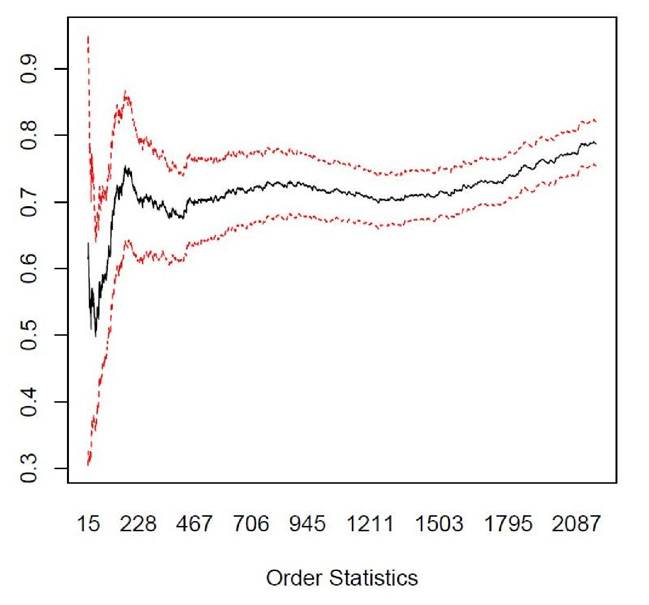
For comparison, we calculated the tail index by using other methods. To be more exact we fitted a generalized extreme value model for the maxima of losses and Pareto distribution over the threshold . The chosen values satisfies the ”not too high, not too low” rule, which is required for the extreme value modeling. Moreover, we estimated the tail index parameter with the Hill estimation by using double bootstrap and Kolmogorov-Smirnov methods. The results can be seen in Table 10. Beside that Figure 4 presents the Hill estimation using different as threshold of ordered statistics.
| Method | Tail index () |
|---|---|
| Fitted GEV | 0.507 |
| Fitted GPD | 0.659 |
| Kolmogorov-Smirnov | 0.61 |
| Double bootstrap | 0.707 |
As one can see, our estimators are between the Kolmogorov-Smirnov and the double bootstrap methods. Using higher subsample size results in lower values. In theory the subsample ratio has to tend to , therefore the estimations from smaller subsample sizes must be closer to the real parameter. One can see, that the estimation is near to the result of the double bootstrap. This observation corresponds to the fact that for the double bootstrap method is more accurate than the one based on the Kolmogorov-Smirnov distance.
With the result of regression fitting method using subsamples of size , we estimated the quantiles of the generalized Pareto distribution with shape parameter . By setting the above value for the shape and as the location parameter, the maximum likelihood estimation for scale is .
Table 11 contains the calculated quantiles of the GPD. Moreover we calculated the empirical distribution function for the quantile values. One can see, that the high quantile estimators are close to the observed quantiles of the fire loss data.
| Quantile | estimated Pareto (emp. dist.) | Empirical quantiles |
|---|---|---|
| 0.95 | 8.68 (0.943) | 9.97 |
| 0.99 | 27.156 (0.99) | 26.04 |
| 0.999 | 124.66 (0.9986) | 131.55 |
4 Conclusion
Our new regression method (3.1) provides an opportunity to estimate the tail index for heavy-tailed distributions. We have shown its merits by the parameter estimation of known distributions, and presented that our method is also useful for real life data. The computation time is less than using the double bootstrap method. However as our algorithm also applies bootstrap techniques, one can use less bootstrap samples to lower the computation time further if needed – at the expense of the estimations’ accuracy, or conversely.
Our simulations showed in consort of Danielsson et al. (2016) that the best estimation is based on the Kolmogorov-Smirnov distance (2.2), if the parameter is less than . For the regression estimation can result the best estimation. However, for higher tail index the methods have a slight dependence of the initial distribution. If the distribution is close to GPD or Student, then the double bootstrap method (2.1) could result more accurate estimation. In contrast, if the distribution is stable or Frechet we recommend to use the regression estimation. Therefore a fast Hill estimation using the Kolmogorov-Smirnov method and fitting distributions for the sample can help to choose the best method for estimating the tail index. This model selection algorithm could be extended by comparing more methods or by more fitted distributions.
Our regression estimation has two types, using the mean of the bootstrap samples or using the location parameter of the best fitted GEV distribution. Our experiments did not indicate which one is the more precise, therefore we suggest using both in a real life analysis. Further calculations could find the answer for this question.
5 Acknowledgment
The project was supported by the European Union, co-financed by the European Social Fund (EFOP-3.6.3-VEKOP-16-2017-00002).
References
- Balkema and de Haan (1974) Balkema, A. and de Haan, L., 1974. Residual life time at great age, Annals of Probability, 2, 792-804.
- Bickel et al. (1997) Bickel, P. J., Götze, F. and van Zwet, W. R., 1997. Resampling fewer than observations:gains, losses and remedies on losses, Statistica Sinica, 7, 1-31.
- Bickel and Sakov (2008) Bickel, P. J. and Sakov, A., 2008. On the choice of in the out of bootstrap and confidence bounds for extrema, Statistica Sinica, 18, 967-985.
- Danielsson et al. (2016) Danielsson, J., Ergun, L. M., De Haan, L. and de Vries, C. G., 2016. Tail Index Estimation: Quantile Driven Threshold Selection, Available at SSRN: https://ssrn.com/abstract=2717478.
- Danielsson et al. (2001) Danielsson, J., de Haan, L., Peng, L. and de Vries, C. G., 2001. Using a bootstrap method to choose the sample fraction in tail index estimation, Journal of Multivariate Analysis, 76, 226-248.
- Davison and Smith (1990) Davison, A. C. and Smith, R. L., 1990. Models for exceedances over high thresholds, Journal of the Royal Statistical Society. Series B (Methodological), 52, 393-442.
- Del Castillo and Padilla (2016) Del Castillo, J. and Padilla, M., 2016. Modeling extreme values by the residual coefficient of variation, SORT–Statistics and operations research transactions, 40, 303-320.
- Fisher and Tippet (1928) Fisher, R. A. and Tippett, L. H. C., 1928. Limiting forms of the frequency distribution of the largest or smallest member of a sample, Mathematical Proceedings of the Cambridge Philosophical Society, 24, 180-190.
- Hill (1975) Hill, B. M., 1975. A simple general approach to inference about the tail index, Annals of Statistics, 3, 1163-1174.
- Hall (1982) Hall P., 1982. On some simple estimates of an exponent of regular variation, Journal of the Royal Statistical Society. Series B (Methodological), 44, 37-42
- Leadbetter (1991) Leadbetter, M. R., 1991. On a basis for ’Peaks over Threshold’ modeling, Statistics & Probability Letters, 12, 357-362.
- Pickands (1975) Pickands, J., 1975. Statistical inference using extreme order statistics, Annals of Statistics, 3, 119-131.
- Resnick (1997) Resnick, S. I., 1997). Discussion Of The Danish Data On Large Fire Insurance Losses, Astin Bulletin 27, 139-151.
- Qi (2008) Qi, Y., 2008. Bootstrap and empirical likelihood methods in extremes, Springer, 11, 81-97.