Electron and proton heating in trans-relativistic magnetic reconnection Note: Accepted to ApJ: October 11, 2017

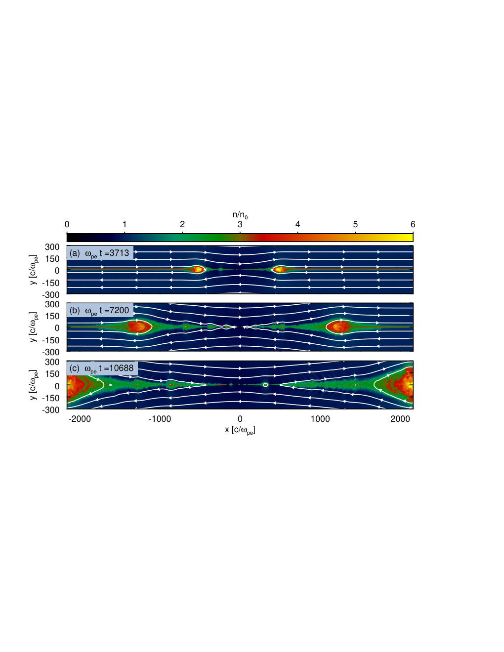
To illustrate the time evolution of the reconnection layer, we show in Fig. 2 a few snapshots of density from a representative simulation (A[0] in Tab. 1) with $\beta_{\rm i}=0.0078$ and $T_{\rm e}/T_{\rm i}=0.1$. We plot the 2D profile of the number density in units of the initial value, $n/n_{0}$. In each panel, we show only a small fraction of the domain in the $y$ direction (we present only the region closest to the current sheet), and the full extent of the domain in $x$. White lines with arrows show magnetic field lines.

Panels (a)–(c) show the time evolution of the system over $\sim 1$ Alfvénic crossing time. By removing by hand the plasma pressure at the center of the current sheet ($x\sim 0$), we trigger a local collapse of the layer, forming an X-point. After the formation of the central X-point, two reconnection “wavefronts” are pulled outwards in the $\pm\mathbf{\hat{x}}$ directions by the magnetic tension of the field lines, and the fronts recede from the center at close to the Alfvén speed. In panels (a), (b), and (c), the wavefronts are located at $x\approx\pm 400,1100,$ and $1800\,c/\omega_{\rm pe},$ respectively, corresponding to the innermost (i.e., closest to $x=0$) locations of the large semi-circular red/yellow density blobs.

The fronts carry away the hot particles initialized in the current sheet. With periodic boundary conditions, this leads to the formation of a primary island at the boundary of the simulation domain (in Fig. 2(c), located at $x\approx\pm 2200\,c/\omega_{\rm pe}).$ The primary island continues to accrete plasma as the system evolves, but eventually it grows so large that further accretion of magnetic flux into the layer is inhibited, and reconnection stops.

The primary island shows the hottest electron temperatures. Here, electron heating might be due in part to reconnection, but also in part to weak shocks at the interface between the reconnection outflow and the island. In addition, the plasma conditions in the island are sensitive to our arbitrary choice for the current sheet initialization. For these reasons, we choose not to focus on the heating physics in the primary island.

In this paper, we focus exclusively on the outflow (i.e., before the the plasma reaches the primary island; see also Shay et al. [35], in the context of non-relativistic reconnection), shown by the green region between the two wavefronts in Fig. 2. In Section III.2, we detail the steps we take to avoid contamination of our temperature measurements by the primary island.

As the two reconnection fronts recede from the center, plasma flows into the reconnection layer and particles are heated and accelerated as a bulk, flowing along $\pm\mathbf{\hat{x}}$ toward the domain boundaries. The dense (green) region in between the two wavefronts is the reconnection outflow. A key feature of low-$\beta_{\rm i}$ simulations is the formation in the reconnection exhausts of secondary islands due to the secondary tearing instability, e.g., Fig. 2(c) at $x\approx 300\,c/\omega_{\rm pe}$ and $x\approx-900\,c/\omega_{\rm pe}$ [7, 43]. Between each pair of secondary islands, there is a secondary X-point, e.g., at $x\approx-1000\,c/\omega_{\rm pe}$. We discuss the structure of the reconnection layer as a function of $\beta_{\rm i}$ in Section IV.1.

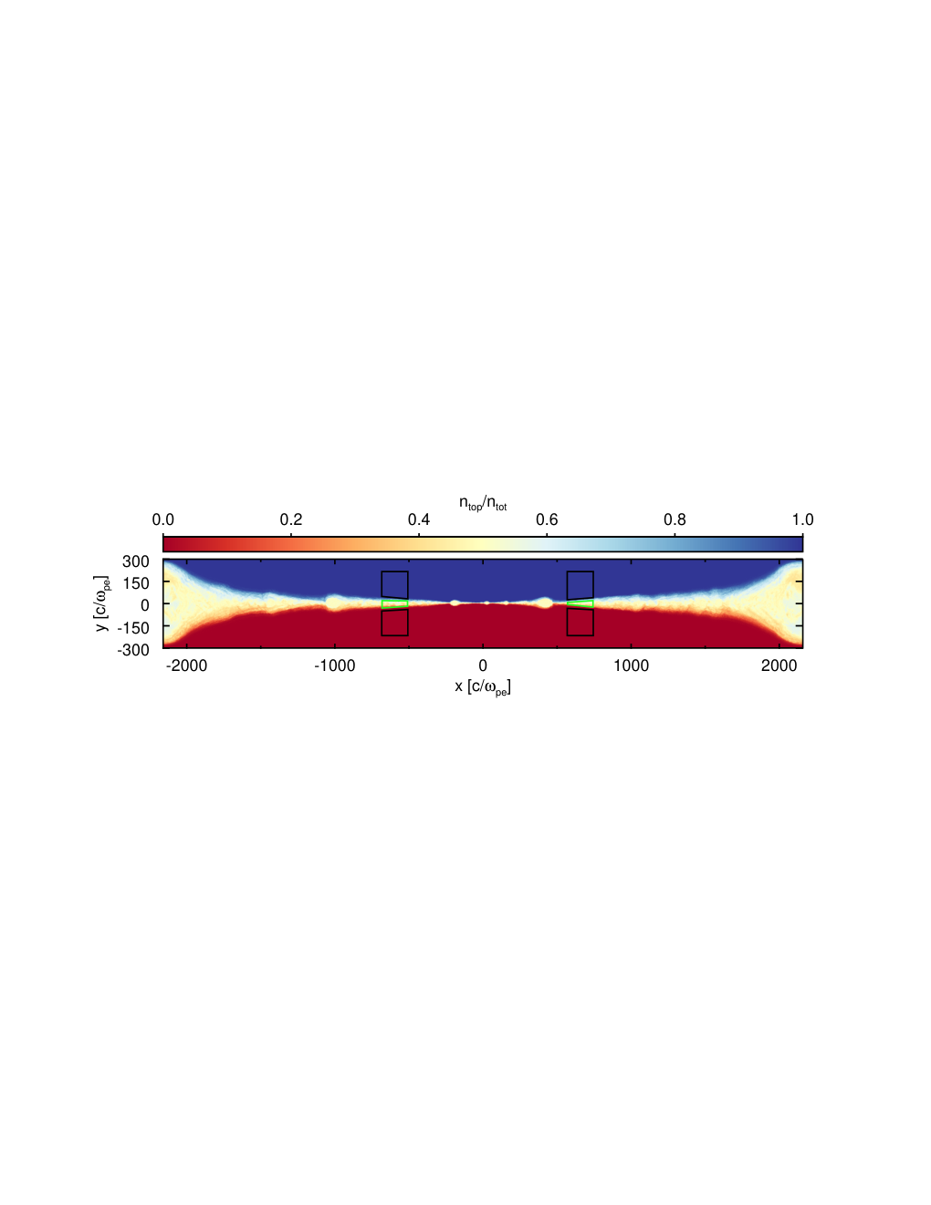
We now describe how we determine which computational cells in the simulation domain belong to the upstream (or, inflow) and downstream (or, outflow) regions. We identify downstream cells by using a particle mixing criterion between the two sides of the current sheet. Particles that originate above $y=0$ (top of the domain) are tagged, to distinguish them from particles originating below $y=0$ (bottom of the domain).

In Fig. 3, we show the ratio of top-to-total number density. Away from the current sheet, i.e., in the blue and red regions, there is no mixing between the two populations. Particles from the two sides of the current sheet get mixed as they enter the reconnection layer; the region with the greatest amount of mixing is shown in white/light-yellow. We compute the ratio of top-particle density $n_{\rm top}$ to total-particle density $n_{\rm tot}=n$ (including particles from both top and bottom) in each cell. If this ratio in a given cell exceeds a chosen threshold $r_{\rm down}$ and is below the complementary threshold, i.e.,

then the cell is counted as one where plasma has reconnected (i.e., the cell belongs to the reconnection downstream). This technique is similar to that used in Daughton et al. [8]. In our analysis, we choose $r_{\rm down}=0.3,$ but we have verified that the identification of the reconnection region, and therefore the heating efficiencies that we extract, do not significantly depend on this choice. For $r_{\rm down}$ in the range $0.1$ – $0.3$, the heating efficiencies typically differ only by $\sim 15\%.$ The choice $r_{\rm down}=0.3$ is restrictive enough to exclude contamination by the upstream region. This is especially important for high $\beta_{\rm i}$, where, even if the electron gyrocenter is located in a cell that is safely part of the downstream, if the cell is close to the interface between downstream and upstream, the particle gyro-motion may temporarily lead this “downstream” electron to the upstream side. If $r_{\rm down}$ were to be too small, the region where the electron motion extends into the upstream might be incorrectly counted as part of the downstream, biasing our temperature estimates toward lower values. Our choice of $r_{\rm down}$ is to some extent arbitrary, but we have found that a relatively large value like $r_{\rm down}=0.3$ is suitable for identifying the genuine reconnection downstream.

In Fig. 4, we show 1D plots of the density fraction of tagged particles and the temperature profiles along the $y$ direction, in a slice located at $x\approx 1000\,c/\omega_{\rm pe}.$ In panel (a), we show the profiles of the ratio of top- and bottom-density to total density, denoted by solid and dashed lines, respectively, at time $t\approx 8400\,\omega_{\rm pe}^{-1}\approx 0.60\,t_{\rm A}$. Between the two vertical dotted lines, the ratio of top-to-total density ranges between 0.3 and 0.7, as required to satisfy our mixing criterion. As shown in panel (b), both the electron (blue) and the proton (red) temperature in the region between the vertical lines are remarkably uniform, proving that our mixing criterion can confidently capture the reconnection downstream.

The upstream region is identified via

and we choose $r_{\rm up}=3\times 10^{-5}$. As before, this definition avoids contamination of the upstream region by any “downstream” particles that leak out of the current sheet. In practice, a buffer zone with a width on the order of a few tens of $c/\omega_{\rm pe}$ is established between the regions we identify as upstream and downstream.

While Eq. 7 (Eq. 8, respectively) identifies the whole reconnection outflow (inflow, respectively), we enforce an additional constraint on the downstream and upstream regions that we employ to extract our heating efficiencies. We select downstream regions far enough from the central X-point that the electron and proton outflow bulk velocities have saturated, and also that the electron and proton temperatures have reached their asymptotic values. At the same time, we select these regions to be far enough from the boundaries to avoid contamination from the material inside the primary island, and only capture the genuine reconnection outflow. The downstream region that satisfies these constraints (identified by the green contours in Fig. 3) varies for different simulations: for $\beta_{\rm i}<2$ it is located at a distance of $\sim 630\,c/\omega_{\rm pe}$ from the center, whereas for $\beta_{\rm i}=2$ it is at $\sim 350\,c/\omega_{\rm pe}$ from the center (as we show below, the primary island tends to be larger at higher $\beta_{\rm i}$). The extent of the downstream region across the layer (i.e., along $y$) is determined by the mixing criterion in Eq. 7, while the length along the layer is fixed at $\sim 170\,c/\omega_{\rm pe}$ (see the green contours in Fig. 3). The corresponding upstream values are measured at the same distance from the center of the layer, within the black contours in Fig. 3. Their exent along the $y$ direction does not significantly affect our results.

In this section, we describe our assessment of particle heating. First, in Section III.3.1, we describe our calculation of rest-frame internal energy and temperature. Next, in Section III.3.2, we define ratios that characterize the total amount of heating. Finally, in Section III.3.3, we provide a more detailed analysis of the heating physics by isolating the effect of a genuine entropy increase (which we call “irreversible heating”) from the contribution of adiabatic compression (giving “adiabatic heating”).

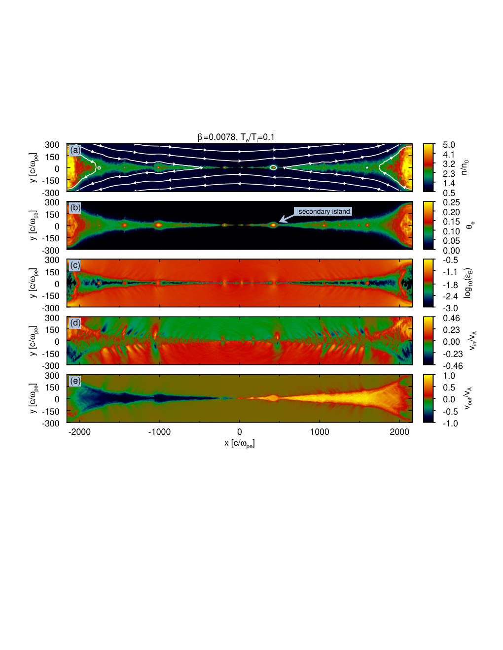
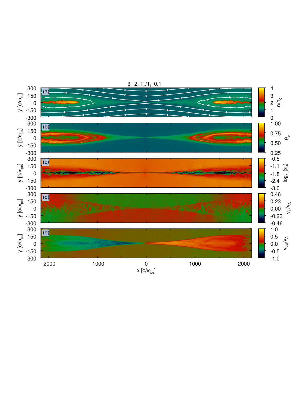
The physics of reconnection shows a marked difference between low- and high-$\beta_{\rm i}$ regimes. In Figs. 5 and 6, we present various fluid quantities for representative low- and high-$\beta_{\rm i}$ simulations, respectively ($\beta_{\rm i}=0.0078$ in Fig. 5 and $\beta_{\rm i}=2$ in Fig. 6). In both cases, $\sigma_{w}=0.1$, $T_{\rm e}/T_{\rm i}=0.1$ and $m_{\rm i}/m_{\rm e}=25$. At $t=11250\,\omega_{\rm pe}^{-1}\approx 0.75\,t_{\rm A}$, we show 2D plots of: (a) the total density in the simulation frame in units of the initial density, $n/n_{0}$; (b) the dimensionless electron temperature $\theta_{\rm e}$; (c) the magnetic energy fraction $\varepsilon_{B}=B^{2}/8\pi n_{0}m_{\rm i}c^{2}$; (d) the inflow velocity $v_{\rm in}/v_{\rm A}=\mathbf{v}\cdot\mathbf{\hat{y}}/v_{\rm A}$ ($v_{\rm A}$ is the Alfvén speed), and (e) the outflow velocity $v_{\rm out}/v_{\rm A}=\mathbf{v}\cdot\mathbf{\hat{x}}/v_{\rm A}$.

A striking difference between the simulations shown in Figs. 5 and 6 is that, while the reconnection outflow at high $\beta_{\rm i}$ is nearly homogeneous, a number of secondary magnetic islands appear at low $\beta_{\rm i}$ (see Fig. 5(a)). The secondary islands are over-dense, and at their center they can reach temperatures a few times larger than the bulk of the outflow (Fig. 5(b)). They also correspond to peaks in magnetic energy (Fig. 5(c)).

The difference in electron temperature between inflow and outflow regions is more pronounced in the low- than in the high-$\beta_{\rm i}$ case (compare Figs. 5(b) and 6(b)). However, as we demonstrate in Section IV.3, the fraction of available magnetic energy converted into total electron heating is roughly comparable between the two cases.

The inflow velocity $v_{\rm in}/v_{\rm A}=\mathbf{v}\cdot\mathbf{\hat{y}}/v_{\rm A}$ is shown in panel (d). For low-$\beta_{\rm i}$, the inflow velocity is $|v_{\rm in}|/v_{\rm A}\approx 0.08.$ It is nearly uniform in the upstream, with the exception of the regions ahead of the secondary islands, where the velocity reverses its sign relative to the ambient inflow (see, e.g., Fig. 5(d) at $x\approx-1100\,c/\omega_{\rm pe}).$ This reversal occurs as the secondary island moves along the outflow direction, pushing aside the inflowing plasma. For high-$\beta_{\rm i},$ the plasma inflow is remarkably uniform, with $|v_{\rm in}|/v_{\rm A}\approx 0.04,$ which is half the value of the low-$\beta_{\rm i}$ case. The inflow velocity at high $\beta_{\rm i}$ shows no reversals near the reconnection exhausts, as there are no secondary islands.

The outflow velocity $v_{\rm out}/v_{\rm A}=\mathbf{v}\cdot\mathbf{\hat{x}}/v_{\rm A}$ is shown in panel (e). For low-$\beta_{\rm i},$ the outflow speed nearly reaches the Alfvén limit, $|v_{\rm out}|/v_{\rm A}\approx 1$, whereas for high-$\beta_{\rm i}$ it approaches a smaller value, $|v_{\rm out}|/v_{\rm A}\approx 0.6.$ For both low and high $\beta_{\rm i},$ the outflow velocity is nearly uniform in the reconnection exhausts, but it drops close to the periodic boundaries at $x\approx\pm 2200,$ as the outflowing plasma accretes onto the primary island.

We show in Fig. 7 a direct comparison between one low-$\beta_{\rm i}$ and one high-$\beta_{\rm i}$ simulation. The left column in Fig. 7 refers to $\beta_{\rm i}=0.0078$ (the same as in Fig. 5), whereas $\beta_{\rm i}=0.5$ for the right column. In both cases, $\sigma_{w}=0.1$, $T_{\rm e}/T_{\rm i}=0.1$ and $m_{\rm i}/m_{\rm e}=25$. In the top row, we show the profile along $x$ of the outflow velocity, for protons (red) and electrons (blue). We find that electrons move slightly faster than protons in the vicinity of the central X-point, but at larger distances the speeds of the two species are the same, and they saturate at a fixed fraction of the Alfvén limit. We show in the middle row of panels the $x$-profile of the dimensionless electron temperature $\theta_{\rm e}$, in the upstream (magenta) and downstream (green). The secondary magnetic islands present in the low-$\beta_{\rm i}$ simulation (panel (c)) are correlated with spikes in the downstream electron temperature (see the peak at $x\approx-500\,c/\omega_{\rm pe}$ in Fig. 7(b)). Aside from the temperature spikes at low $\beta_{\rm i}$, the two panels in the middle row of Fig. 7 demonstrate that, far enough from the central X-point, the electron temperature is nearly uniform.

To estimate the reconnection heating efficiency, we measure the downstream temperature in the two slabs delimited by the vertical dotted lines in Fig. 7(b) and (e) (more precisely, within the green contours in Fig. 3). The time evolution of the total electron heating efficiency $M_{T\rm e,tot}$, of the adiabatic contribution $M_{T\rm e,ad}$ and of the irreversible component $M_{T\rm e,irr}$ are shown in Fig. 8 with black, dashed blue and dashed red lines, respectively. The top panel refers to a low-$\beta_{\rm i}$ simulation with $\beta_{\rm i}=0.0078$, whereas the bottom panel refers to the high-$\beta_{\rm i}$ case $\beta_{\rm i}=2$. In both cases, $\sigma_{w}=0.1$, $T_{\rm e}/T_{\rm i}=0.1$ and $m_{\rm i}/m_{\rm e}=25$. The horizontal axis in the figure starts from $t=5000\,\omega_{\rm pe}^{-1}$, which corresponds to the time when the two reconnection wavefronts pass beyond the region that we employ for calculating the downstream quantities (as discussed above, after this time the measurements are no longer affected by our choice of initialization of the current sheet).¹¹ 1 This time is typically in the range $t\approx 4000-5000\,\omega_{\rm pe}^{-1}$, with marginal dependence on $\beta_{\rm i}$ and on the initial sheet thickness $\Delta$. While the heating efficiencies are nearly constant in time for high $\beta_{\rm i}$ (bottom panel), the temporal profiles at low $\beta_{\rm i}$ (top panel) present quasi-periodic modulations. They mark the passage of secondary islands — whose temperature is typically hotter than the bulk outflow — through the region used for our computations. To minimize the temperature variations associated with secondary islands, we average the heating efficiencies over time, as described in Section III.3.2. In doing so, the results we obtain are a reliable assessment of the steady-state heating physics in reconnection.

Panels (a) and (b) in Fig. 8 also demonstrate that the fractional contributions of adiabatic and irreversible heating to the total electron heating significantly depend on $\beta_{\rm i}$, as we further discuss in Section IV.3. In the low-$\beta_{\rm i}$ regime, adiabatic heating is unimportant as compared to the irreversible part, whereas the two components are comparable at high $\beta_{\rm i}$.

In Fig. 9, we show the dependence on $\beta_{\rm i}$ and $T_{\rm e}/T_{\rm i}$ of various fluid quantities, from a suite of simulations with fixed $\sigma_{w}=0.1$ and $m_{\rm i}/m_{\rm e}=25$. We present the (a) inflow velocity normalized to the Alfvén speed $|v_{\rm in}|/v_{\rm A}$; (b) outflow velocity normalized to the Alfvén speed $|v_{\rm out}|/v_{\rm A}$; (c) ratio of inflow to outflow velocity $|v_{\rm in}|/|v_{\rm out}|$; (d) downstream rest-frame density in units of the initial density in the upstream $\bar{n}_{\rm down}/n_{0}$; (e) width of the reconnection region at a distance of $430\,c/\omega_{\rm pe}$ from the center of the layer. Blue, green, and red points denote simulations with upstream temperature ratios $T_{\rm e}/T_{\rm i}=0.1,0.3,$ and $1,$ respectively.

As described in Section III.3.2, the quantities we extract are time-averaged, typically over 0.3 Alfvénic crossing times, corresponding to $\sim 4500\,\omega_{\rm pe}^{-1}.$ The points in Fig. 9 represent the time averages, with vertical error bars indicating one standard deviation. At low $\beta_{\rm i},$ the inflow velocity is $|v_{\rm in}|/v_{\rm A}\approx 0.08,$ independent of the upstream temperature ratio (panel (a)). In the high-$\beta_{\rm i}$ case, the inflow speed is smaller, $|v_{\rm in}|/v_{\rm A}\approx 0.04$, and shows a weak dependence on the temperature ratio, with higher temperature ratios attaining lower values of $|v_{\rm in}|/v_{\rm A}$.

The outflow velocity (panel (b)) nearly saturates the Alfvén limit at low $\beta_{\rm i}$ (the Alfvén limit is indicated with the horizontal dashed black line), whereas for high $\beta_{\rm i}$ it is sub-Alfvénic, $|v_{\rm out}|/v_{\rm A}\approx 0.75$. For low values of $\beta_{\rm i}$, i.e., $\beta_{\rm i}\lesssim 0.1,$ the outflow velocity is nearly independent of the temperature ratio, whereas at high $\beta_{\rm i}$ it shows a weak dependence on $T_{\rm e}/T_{\rm i}$, with higher temperature ratios corresponding to greater outflow speeds.

The dependence of the reconnection rate $|v_{\rm in}|/|v_{\rm out}|$ on $\beta_{\rm i}$ and $T_{\rm e}/T_{\rm i}$ (panel (c)) follows from the variations in inflow speed and outflow velocity that we have just discussed. At low $\beta_{\rm i},$ the reconnection rate is $|v_{\rm in}|/|v_{\rm out}|\approx 0.08$ regardless of the temperature ratio, whereas at high $\beta_{\rm i}$, and specifically for $\beta_{\rm i}=2,$ the reconnection rate at $T_{\rm e}/T_{\rm i}=1$ is $|v_{\rm in}|/|v_{\rm out}|\approx 0.04,$ only half that of the $T_{\rm e}/T_{\rm i}=0.1$ case. So, in the high-$\beta_{\rm i}$ regime reconnection proceeds slower for hotter upstream electrons.

As $\beta_{\rm i}$ increases, the plasma is less prone to be compressed during the reconnection process. As shown in Fig. 9 (d), the downstream to upstream density ratio decreases as $\beta_{\rm i}$ increases. The value of $\hbox to0.0pt{\hskip 0.50116pt\hbox{$\overline{\hbox{}}$}\hss}{\hbox{$n$}}_{\rm down}/n_{0}$ is nearly independent of the upstream temperature ratio. Though the ratio $\hbox to0.0pt{\hskip 0.50116pt\hbox{$\overline{\hbox{}}$}\hss}{\hbox{$n$}}_{\rm down}/n_{0}$ approaches unity at high $\beta_{\rm i},$ this does not necessarily imply that the fractional contribution of adiabatic heating to total heating is negligible at high $\beta_{\rm i}$ (we demonstrate this in Section IV.3).

Lastly, in panel (e) we show the $\beta_{\rm i}$-dependence of the reconnection layer width $\delta_{\rm rec},$ in units of the electron skin depth $c/\omega_{\rm pe}$. We measure the width across the reconnection layer, as identified by Eq. 7, at a distance $\sim 430\,c/\omega_{\rm pe}$ downstream of the central X-point. The width shows strong variability in time at low $\beta_{\rm i}$, as secondary islands pass through the region employed for our measurements (note the large error bars). Despite the uncertainty in the measurement, panel (e) shows a consistent trend of increasing reconnection layer width $\delta_{\rm rec}$ with $\beta_{\rm i}$. The measured values of $\delta_{\rm rec}$ lie in the range $25$ – $50\,c/\omega_{\rm pe},$ which is apparently close to the chosen current sheet thickness at initialization, $\Delta=40\,c/\omega_{\rm pe}.$ However, we demonstrate in Appendix F that the measured reconnection layer width is independent of our choice of the initial sheet thickness. It follows that our measurement leads to a reliable assessment of the opening angle of the reconnection outflow, $\sim\delta_{\rm rec}/(430\,c/\omega_{\rm pe})\sim 0.1$.

In Fig. 10, we show the $\beta_{\rm i}$ and $T_{\rm e}/T_{\rm i}$ dependence of electron (panel (a)) and proton (panel (b)) dimensionless temperature, and the ratio of proton-to-electron skin depth (panel (c); see Eq. 5). In each panel, solid and dashed lines indicate downstream and upstream quantities, respectively. As in Fig. 9, blue, green, and red points refer to electron-to-proton temperature ratios $T_{\rm e}/T_{\rm i}=0.1,0.3$, and $1$, respectively. The upstream electron dimensionless temperatures lie in the range $10^{-3}$ to $10$, as in Table 1; for protons, the dimensionless temperature in the upstream ranges from $4\times 10^{-4}$ to $0.4$.

The range of temperatures in the downstream is smaller than in the upstream (compare the solid and dashed lines in Fig. 10(a) and (b)). At low $\beta_{\rm i}$, the available magnetic energy is large compared to the particle thermal content in the upstream, so dissipation of the magnetic field leads to electron and proton temperatures in the downstream that are nearly independent of $\beta_{\rm i}$. At high $\beta_{\rm i}$, the energy transferred from the fields to the particles is much smaller than the initial particle thermal content, giving a minor increase of temperature from upstream to downstream. Even if the fractional increase in temperature is extremely small at high $\beta_{\rm i}$, the fraction of available magnetic energy being converted into particle heating might still be as large as at low $\beta_{\rm i}$. The rest of the section addresses this question.

We show the plasma-$\beta_{\rm i}$ and temperature ratio $T_{\rm e}/T_{\rm i}$ dependence of electron and proton heating in Fig. 11. The simulations presented here are those referenced in Tab. 1, for which $m_{\rm i}/m_{\rm e}=25$ and $\sigma_{w}=0.1$. We indicate the total, adiabatic, and irreversible heating by $M_{T\rm e,tot}$ (Eq. 16), $M_{T\rm e,ad}$ and $M_{T\rm e,irr}$ (Eqs. 23) for electrons, and by $M_{T\rm i,tot}$ (Eq. 18), $M_{T\rm i,ad}$ and $M_{T\rm i,irr}$ (Eqs. 25) for protons. Blue, green, and red points indicate simulations with upstream electron-to-proton temperature ratios of $0.1,0.3,$ and $1$, respectively. As in Section IV.2, filled points are the time-averaged results of our simulations, and vertical error bars indicate one standard deviation from the mean. The top, middle, and bottom rows show heating fractions of electrons, protons, and of the overall fluid, respectively, which we now discuss in turn.

In Fig. 11(a), we show the dependence of the total electron heating efficiency $M_{T\rm e,tot}$ on $\beta_{\rm i}$ and $T_{\rm e}/T_{\rm i}$. Although the initial plasma $\beta_{\rm i}$ spans more than two orders of magnitude, and the initial temperature ratio an order of magnitude, even the most extreme values of $M_{T\rm e,tot}$ differ by no more than a factor of $\sim 4$. The value of $M_{T\rm e,tot}$ in our $\beta_{\rm i}\lesssim 0.5$ simulations, for which electrons stay non-relativistic both in the upstream and in the downstream, is $\sim 0.04,$ which is consistent with the results of non-relativistic reconnection by Shay et al. [35] for mass ratio $m_{\rm i}/m_{\rm e}=25$.²² 2 In Shay et al. [35], the magnetization was $\sigma_{w}\approx 0.004-0.1$. However, as long as $\sigma_{w}\ll 1$ and all the species stay at non-relativistic temperatures, we expect the reconnection physics to be independent of the flow magnetization. As shown by Shay et al. [35], the electron heating efficiency in non-relativistic reconnection is expected to decrease with increasing mass ratio; in Sections IV.4 and IV.6, we present the dependence of the electron and proton heating fractions in trans-relativistic reconnection on $m_{\rm i}/m_{\rm e}$, up to the physical value.

The total electron heating fraction $M_{T\rm e,tot}$ is decomposed into adiabatic and irreversible components in panels (b) and (c). By comparing the two panels, we see that most of the heating in the low-$\beta_{\rm i}$ regime comes from irreversible processes, i.e., it is accompanied by a genuine increase in entropy, while heating at high $\beta_{\rm i}$ mostly results from adiabatic compression.

The electron adiabatic heating efficiency increases with the inflow temperature ratio $T_{\rm e}/T_{\rm i}$ (Fig. 11(b)). The dependence is most apparent at high $\beta_{\rm i},$ where adiabatic heating represents a significant contribution to the total heating. The dependence of adiabatic heating on temperature ratio can be simply understood through the adiabatic law $T/\hbox to0.0pt{\hskip 0.50116pt\hbox{$\overline{\hbox{}}$}\hss}{\hbox{$n$}}^{\hat{\gamma}-1}=\text{const.}$ As electrons get compressed from upstream to downstream, the adiabatic heating fraction can be written as³³ 3 Eq. 27 assumes that the adiabatic index is constant as electrons pass from upstream to downstream, which is a good approximation when electrons are ultra-relativistic in both regions (so, for high $\beta_{\rm i}$ and large $T_{\rm e}/T_{\rm i}$); still, in all the simulations used in Fig. 11, we find that the electron adiabatic index changes by no more than $\hat{\gamma}_{\rm e,up}-\hat{\gamma}_{\rm e,down}\approx 0.1$. In any case, Eq. 27 is presented only for illustrative purposes, and we properly account for the effect of a variable adiabatic index in our calculation of the heating fractions.

As shown in Fig. 9(d), the ratio of downstream to initial upstream density $\hbox to0.0pt{\hskip 0.50116pt\hbox{$\overline{\hbox{}}$}\hss}{\hbox{$n$}}_{\rm down}/n_{0}$ is nearly independent of the upstream temperature ratio, so that $M_{T\rm e,ad}\propto T_{\rm e}/T_{\rm i}$ at fixed $\beta_{\rm i}$. Eq. 27 also provides insight into the $\beta_{\rm i}$-dependence of adiabatic heating. It shows that, for a given temperature ratio, the adiabatic heating efficiency would scale linearly with $\beta_{\rm i}$, if the compression ratio $\hbox to0.0pt{\hskip 0.50116pt\hbox{$\overline{\hbox{}}$}\hss}{\hbox{$n$}}_{\rm down}/n_{0}$ were to be fixed. As shown in Fig. 9(d), the downstream to upstream density ratio decreases with $\beta_{\rm i}$, approaching unity at high $\beta_{\rm i}$. However, the decrease of $\hbox to0.0pt{\hskip 0.50116pt\hbox{$\overline{\hbox{}}$}\hss}{\hbox{$n$}}_{\rm down}/n_{0}$ with $\beta_{\rm i}$ is quite shallow, and insufficient to counteract the linear dependence on $\beta_{\rm i}$ in Eq. 27. It follows that at low $\beta_{\rm i}$ the effect of adiabatic heating is negligible, while at high $\beta_{\rm i}$ the role of adiabatic heating can be more important than that of irreversible heating.

This statement can be further justified by considering electron energization in the diffusion region as the main source of irreversible electron heating, following Le et al. [14]. In the diffusion region, the electron energy will increase by $eE_{\rm rec}\ell_{\rm e}$, where $E_{\rm rec}\sim 0.1(v_{\rm A}/c)B_{0}$ is the reconnection electric field (assuming a reconnection inflow rate of $\sim 0.1\,v_{\rm A}/c$, see Fig. 9(a)) and $\ell_{\rm e}$ is the distance traveled by electrons along the electric field (along $z$, in our geometry). For the sake of simplicity, let us now assume that $\beta_{\rm i}$ is sufficiently small that $w\sim n_{0}m_{\rm i}c^{2}$ and so $\sigma_{w}\sim\sigma_{\rm i}$ (this is the case for $\beta_{\rm i}\lesssim 0.1$, at our reference magnetization $\sigma_{w}=0.1$). The corresponding irreversible heating efficiency can be written in the case $\sigma_{w}\sim\sigma_{\rm i}\lesssim 1$ as

which does not depend explicitly on $\beta_{\rm i}$. It follows that, as long as $\ell_{\rm e}$ is a weak function of $\beta_{\rm i}$, the adiabatic heating efficiency in Equation 27, which scales linearly with $\beta_{\rm i}$, will be unimportant at low $\beta_{\rm i}$, whereas it will dominate over irreversible heating at high $\beta_{\rm i}$.

We remark that Equation 28 does not capture a number of important effects. First, by tracking individual particle orbits, we have found that the in-plane components of the electric field, that we have neglected above, can provide a significant contribution to the total electron energization (a comprehensive discussion of the physics of electron heating will be presented elsewhere). Second, we have neglected the $\beta_{\rm i}$-dependence of the reconnection rate. Third, we have assumed $w\sim n_{0}m_{\rm i}c^{2}$, which is incorrect at high $\beta_{\rm i}$. Fourth, we do not have a direct measure of $\ell_{\rm e}$, which would assess its dependence on the flow conditions. For these reasons, it is likely that the electron irreversible heating will be dependent on $\beta_{\rm i}$.

In fact, the irreversible electron heating efficiency (shown in Fig. 11(c)) systematically decreases with $\beta_{\rm i}$, and the trend is largely independent of the initial temperature ratio, apart from the case with $\beta_{\rm i}=2$ (rightmost points in Fig. 11(c)). Here, the irreversible heating fraction reaches $M_{T\rm e,irr}\approx 0.03$ for $T_{\rm e}/T_{\rm i}=1$, a factor of $\sim 3$ larger than for the $\beta_{\rm i}=2$ cases with lower temperature ratios, $T_{\rm e}/T_{\rm i}=0.1$ and 0.3.⁴⁴ 4 We have extensively checked this result, finding that it holds regardless of the simulation boundary conditions (periodic or outflow in the $x$ direction, or double periodic; see Appendix B) and the number of computational particles per cell. We attribute the peculiar behavior of this case to the fact that, among the $m_{\rm i}/m_{\rm e}=25$ simulations presented in Fig. 11, the $\beta_{\rm i}=2,\,T_{\rm e}/T_{\rm i}=1$ case is the only one for which the scale separation $(c/\omega_{\rm pi})/(c/\omega_{\rm pe})$ between protons and electrons approaches unity (see Fig. 10(c)). For the case $\beta_{\rm i}=2,T_{\rm e}/T_{\rm i}=1$ in Fig. 11, this statement holds true for both the upstream and the downstream scale separation, since the reconnection process at high $\beta_{\rm i}$ does not appreciably change the plasma thermal content. However, as we further discuss in the next two subsections, where we investigate the dependence of our results on the mass ratio and the magnetization, we find that the necessary and sufficient condition for the electron and proton heating efficiencies to be comparable is that the downstream scale separation approaches unity. In retrospect, this is not surprising, since if $(c/\omega_{\rm pi})/(c/\omega_{\rm pe})\rightarrow 1$ in the downstream, the fluid effectively behaves like an electron-positron plasma.

In Fig. 11 (second row of panels), we also explore the $\beta_{\rm i}$-dependence of (d) total, (e) adiabatic, and (f) irreversible proton heating. As before, blue, green, and red points correspond to simulations with upstream $T_{\rm e}/T_{\rm i}$ of $0.1,0.3,$ and $1,$ respectively (we change the temperature ratio by varying the electron temperature, while the proton temperature at a given $\beta_{\rm i}$ is kept fixed). While the initial dimensionless electron temperature in our simulations ranges from non-relativistic to ultra-relativistic values, protons always stay at non-relativistic or trans-relativistic energies, $\theta_{\rm i}\approx 0.0004$ – $0.5$ (this is true in both upstream and downstream). At low $\beta_{\rm i}$, protons are heated more efficiently than electrons, typically by a factor of 2 – 3 at mass ratio $m_{\rm i}/m_{\rm e}=25$ (compare panels (a) and (d), $M_{T\rm e,tot}\approx 0.05$ while $M_{T\rm i,tot}\approx 0.13$). At larger values of $m_{\rm i}/m_{\rm e},$ the ratio of proton to electron heating is even larger, as we discuss in Sections IV.4 and IV.6. Once again, the notable exception is the high-$\beta_{\rm i}$ case with $\beta_{\rm i}=2$ and $T_{\rm e}/T_{\rm i}=1,$ where the electron and proton heating fractions are comparable, $M_{T\rm e,tot}\approx 0.06$ and $M_{T\rm i,tot}\approx 0.08$. Similar to electrons, the irreversible component of proton heating decreases with $\beta_{\rm i},$ and shows only weak dependence on the upstream temperature ratio $T_{\rm e}/T_{\rm i}$ (panel (f)). As shown in panel (e), the fractional contribution of adiabatic heating to the total proton heating increases with $\beta_{\rm i}$, as for electrons.

References

- [1] Abramowicz, M. a. M. M. a., Chen, X., Kato, S., Lasota, J.-P. J.-P., & Regev, O. 1995, Apjl, 438, 8
- [2] Ball, D., Özel, F., Psaltis, D., Chan, C.-k., & Sironi, L. 2017, arXiv:1705.06293v1
- [3] Ball, D., Özel, F., Psaltis, D., & kwan Chan, C. 2016, The Astrophysical Journal, 826, 77
- [4] Buneman, O. 1993, TRISTAN The 3-D electromagnetic particle code
- [5] Chael, A. A., Narayan, R., & Sädowski, A. 2017, Monthly Notices of the Royal Astronomical Society, 470, 2367
- [6] Dahlin, J. T., Drake, J. F., & Swisdak, M. 2014, Physics of Plasmas, 21, 092304
- [7] Daughton, W., & Karimabadi, H. 2007, Physics of Plasmas, 14
- [8] Daughton, W., Nakamura, T. K. M., Karimabadi, H., Roytershteyn, V., & Loring, B. 2014, Physics of Plasmas, 21
- [9] Doeleman, S. S., Weintroub, J., Rogers, A. E. E., et al. 2008, Nature, 455, 78
- [10] Guo, F., Li, X., Li, H., et al. 2016, The Astrophysical Journal, 818, L9
- [11] Haggerty, C. C., Shay, M.A., Drake, J.F., Phan, T. D., & McHugh, C. T. 2015, Geophys. Res. Lett., 42, 9657-9665.
- [12] Hoshino, M., Hiraide, K., & Mukai, T. 2001, Earth, Planets and Space, 53, 627
- [13] Jaroschek, C. H., Treumann, R. A., Lesch, H., & Scholer, M. 2004, Physics of Plasmas, 11, 1151
- [14] Le, A., Egedal, J., & Daughton, W. 2016, Physics of Plasmas, 23, 1
- [15] Li, X., Guo, F., Li, H., & Li, G. 2015, The Astrophysical Journal, 811, L24
- [16] —. 2017, The Astrophysical Journal, 843, 21
- [17] Loureiro, N. F., Schekochihin, A. A., & Zocco, A. 2013, Phys. Rev. Lett., 111, 025002
- [18] Melzani, M., Walder, R., Folini, D., Winisdoerffer, C., & Favre, J. M. 2014, Astronomy & Astrophysics, 570, A111
- [19] Melzani, M., Winisdoerffer, C., Walder, R., et al. 2013, Astronomy & Astrophysics, 558, A133
- [20] Narayan, R., & McClintock, J. E. 2008, New Astronomy Reviews, 51, 733
- [21] Narayan, R., & Yi, I. 1994, The Astrophysical Journal, 428, 1316
- [22] —. 1995a, The Astrophysical Journal, 444, 231
- [23] —. 1995b, The Astrophysical Journal, 452, 710
- [24] Numata, R., & Loureiro, N. F. 2015, Journal of Plasma Physics, 81, 305810201
- [25] Phan, T. D., Shay, M. A., Gosling, J. T., et al. 2013, Geophysical Research Letters, 40, 4475
- [26] Quataert, E., Dorland, W., & Hammett, G. W. 2002, The Astrophysical Journal, 577, 524
- [27] Ressler, S. M., Tchekhovskoy, A., Quataert, E., Chandra, M., & Gammie, C. F. 2015, Monthly Notices of the Royal Astronomical Society, 454, 1848
- [28] Ressler, S. M., Tchekhovskoy, A., Quataert, E., & Gammie, C. F. 2017, Monthly Notices of the Royal Astronomical Society, 467, 3604
- [29] Riquelme, M. A., Quataert, E., Sharma, P., & Spitkovsky, A. 2012, 50
- [30] Riquelme, M. A., Quataert, E., & Verscharen, D. 2015, The Astrophysical Journal, 800, 27
- [31] Sädowski, A., Sironi, L., Abarca, D., et al. 2013, Monthly Notices of the Royal Astronomical Society, 432, 478
- [32] Sädowski, A., Wielgus, M., Narayan, R., et al. 2017, Monthly Notices of the Royal Astronomical Society, 466, 705
- [33] Schoeffler, K. M., Drake, J. F., & Swisdak, M. 2011, The Astrophysical Journal, 743, 70
- [34] Schoeffler, K. M., Drake, J. F., Swisdak, M, & Knizhnik, K. 2013, The Astrophysical Journal, 764, 126
- [35] Shay, M. A., Haggerty, C. C., Phan, T. D., et al. 2014, Physics of Plasmas, 21
- [36] Sironi, L. 2015, The Astrophysical Journal, 800, 89
- [37] Sironi, L., Giannios, D., & Petropoulou, M. 2016, Monthly Notices of the Royal Astronomical Society, 462, 48
- [38] Sironi, L., & Narayan, R. 2015, The Astrophysical Journal, 800, 88
- [39] Sironi, L., Petropoulou, M., & Giannios, D. 2015, Monthly Notices of the Royal Astronomical Society, 450, 183
- [40] Sironi, L., & Spitkovsky, A. 2011, The Astrophysical Journal, 726, 75
- [41] —. 2014, The Astrophysical Journal, 783, L21
- [42] Spitkovsky, A. 2005, AIP Conference Proceedings, 801, 345
- [43] Uzdensky, D. A., Loureiro, N. F., & Schekochihin, A. A. 2010, Physical Review Letters, 105, 16
- [44] Werner, G. R., Uzdensky, D. A., Begelman, M. C., Cerutti, B., & Nalewajko, K. 2016, arXiv:1612.04493
- [45] Yuan, F., & Narayan, R. 2014, Annual Review of Astronomy and Astrophysics, 52, 529
- [46] Yuan, F., Quataert, E., & Narayan, R. 2003, The Astrophysical Journal, 598, 301