Skill of global raw and postprocessed ensemble predictions of rainfall over northern tropical Africa
Abstract
Accumulated precipitation forecasts are of high socioeconomic importance for agriculturally dominated societies in northern tropical Africa. In this study, we analyze the performance of nine operational global ensemble prediction systems (EPSs) relative to climatology-based forecasts for 1 to 5-day accumulated precipitation based on the monsoon seasons 2007–2014 for three regions within northern tropical Africa. To assess the full potential of raw ensemble forecasts across spatial scales, we apply state-of-the-art statistical postprocessing methods in form of Bayesian Model Averaging (BMA) and Ensemble Model Output Statistics (EMOS), and verify against station and spatially aggregated, satellite-based gridded observations. Raw ensemble forecasts are uncalibrated, unreliable, and underperform relative to climatology, independently of region, accumulation time, monsoon season, and ensemble. Differences between raw ensemble and climatological forecasts are large, and partly stem from poor prediction for low precipitation amounts. BMA and EMOS postprocessed forecasts are calibrated, reliable, and strongly improve on the raw ensembles, but – somewhat disappointingly – typically do not outperform climatology. Most EPSs exhibit slight improvements over the period 2007–2014, but overall have little added value compared to climatology. We suspect that the parametrization of convection is a potential cause for the sobering lack of ensemble forecast skill in a region dominated by mesoscale convective systems.
1 Introduction
The bulk of precipitation in the Tropics is related to moist convection, in contrast to the frontal-dominated extratropics. Due to the small-scale processes involved in the triggering and growth of convective systems, quantitative precipitation forecasts are known to have overall poorer skills in tropical latitudes (Haiden et al., 2012). This can be monitored in quasi-real time on the World Meteorological Organisation (WMO) Lead Centre on Verification of Ensemble Prediction System website (http://epsv.kishou.go.jp/EPSv) by comparing deterministic and probabilistic skill scores for 24-hour precipitation forecasts for the N–S tropical belt with those for the northern and southern hemisphere extratropics. There are hints that precipitation and cloudiness forecasts in the Tropics show enhanced skill during regimes of stronger synoptic-scale forcing (Söhne et al., 2008; Davis et al., 2013; van der Linden et al., 2017) or in regions of orographic forcing (Lafore et al., 2017), but large parts of the tropical land masses are dominated by convection that initiates from small-scale surface and boundary layer processes and sometimes organizes into mesoscale convective systems (MCSs). The latter depends mostly on the thermodynamic profile and vertical wind shear.
In this context, northern tropical Africa, particularly the semi-arid Sahel, can be considered a region where precipitation forecasting is particularly challenging. The area consists of vast flatlands, MCSs during boreal summer provide the bulk of the annual rainfall (Mathon et al., 2002; Fink et al., 2006; Houze et al., 2015), and convergence lines in the boundary layer or soil moisture gradients at the km-scale can act as triggers for MCSs (Lafore et al., 2017). Sahelian MCSs often take the form of meridionally elongated squall lines with sharp leading edges characterized by heavy rainfall. Synoptic-scale African easterly waves are known to be linked to squall line occurrence in the western Sahel (Fink and Reiner, 2003) and lead to an enhanced skill of cloudiness forecasts over West Africa (Söhne et al., 2008).
However, numerical weather prediction (NWP) models are known to have an overall poor ability to predict rainfall systems over northern Africa. For example, the gain in skill by improved initial conditions due to an enhanced upper-air observational network during the 2006 AMMA campaign (Parker et al., 2008) was lost in NWP models after 24 hours of forecast time, potentially due to the models’ inability to predict the genesis and evolution of convective systems (Fink et al., 2011).
Given the substantial challenges involved in forecasting rainfall in northern Africa, one might hope that ensemble prediction systems (EPSs) provide a useful assessment of uncertainties and a more useful forecast overall. An ensemble is a set of deterministic forecasts, created by changes in the initial conditions and/or the numerical representation of the atmosphere (Palmer, 2002). With clear advantages of ensembles over single deterministic forecasts, EPSs are now run at all major NWP centers, which led to the creation of the TIGGE multi-model ensemble database (Bougeault et al., 2010; Swinbank et al., 2016). TIGGE contains forecasts from up to ten global EPSs, with the ensemble of the European Centre for Medium-Range Weather Forecasts (ECMWF) being the most prominent and most important contributor (Hagedorn et al., 2012). To our knowledge, this present study is the first to rigorously and systematically assess the quality of ensemble forecasts for precipitation over northern tropical Africa. This is partly related to the fact that for this region ground verification data from rain gauge observations are infrequent on the Global Telecommunication System (GTS), the standard verification data source for NWP centers.
Despite many advances in the generation of EPSs, ensembles share structural deficiencies such as dispersion errors and biases. Statistical postprocessing addresses these deficiencies and thereby allows assessing the full potential of ensemble forecasts (Gneiting and Raftery, 2005). Additionally, it enables fair comparisons between different spatial scales, such as model gridboxes and point observations. The correction of systematic forecast errors is based on (distributional) regression techniques and, depending on the need of the user, several approaches are at hand (Schefzik et al., 2013; Gneiting, 2014). Hamill et al. (2004) and Wilks (2009) proposed and extended logistic regression techniques, which yield probabilistic forecasts for the exceedance of thresholds. Here we will for the first time explore whether established methods such as Bayesian Model Averaging (Raftery et al., 2005, BMA,) and Ensemble Model Output Statistics (Gneiting et al., 2005, EMOS,), which provide complete probabilistic quantitative precipitation forecasts, can improve precipitation forecasts for Africa.
The ultimate goal of this paper is to provide an exhaustive assessment of our current ability to predict rainfall over northern tropical Africa, considering the skill of raw and postprocessed forecasts from TIGGE. Any skill, if existing, would be expected to come from resolved large-scale forcing processes as mentioned above. We examine accumulation periods of 1- to 5-days for the monsoon seasons 2007–2014 and verify against about 21,000 daily rainfall observations from 132 rain gauge stations and satellite-based gridded precipitation observations. Section 2 introduces the TIGGE ensemble, and the station and satellite-based observations used for verification. Section 3 describes our benchmark climatological forecast and methods for the evaluation of probabilistic forecasts, and explains EMOS and BMA in detail. Results are presented in section 4, where we verify 1-day accumulated ECMWF precipitation forecasts against station observations. This analysis is performed in particular depth and serves as fundamental examplar. We also evaluate ECWMF ensemble forecasts at longer accumulation times and for spatial aggregations, before turning to the analysis of all TIGGE sub-ensembles. Implications of our findings and possible alternative methods for forecasting precipitation over northern tropical Africa are discussed in section 5.
2 Data
2.1 Forecasts
The TIGGE multi-model ensemble was set up as part of the THORPEX programme in order to “accelerate improvements in the accuracy of 1-day to 2-week high-impact weather forecasts for the benefit of humanity” (Bougeault et al., 2010, p. 1060). Since its start in October 2006, up to 10 global NWP centers have provided their operational ensemble forecasts, which are accessible on a common grid. Park et al. (2008) and Bougeault et al. (2010) discuss objectives and the set-up of TIGGE, including the participating EPSs, in great detail. They also note early results using the TIGGE ensemble, while Swinbank et al. (2016) report on achievements accomplished over the last decade. Hagedorn et al. (2012) find that a multi-model ensemble composed of the four best participating TIGGE EPSs, which include the ECMWF ensemble, outperforms reforecast-calibrated ECMWF forecasts. For the evaluation of NWP precipitation forecast quality, TIGGE is the most complete and best available data source for the period 2007–2014. Table 1 gives an overview of the nine participating TIGGE EPSs that provide accumulated precipitation forecasts.
In addition to the separate evaluation of each participating TIGGE sub-ensemble, we construct a reduced multi-model (RMM) ensemble. For each of the seven sub-ensembles available for the period 2008–2013, the RMM ensemble uses the mean of the perturbed members, and the control run, and in case of the ECMWF EPS furthermore the high-resolution run, as individual contributors. The RMM ensemble therefore consists of 15 members and, as postprocessing performs an implicit weighting of all contributions, a manual selection of sub-ensembles as performed by Hagedorn et al. (2012) is not necessary.
Arguably, the ECMWF EPS is the leading one among the TIGGE sub-ensembles (Buizza et al., 2005; Hagedorn et al., 2012; Haiden et al., 2012). It consists of a high-resolution (HRES) run, a control (CNT) run, and 50 perturbed ensemble (ENS) members. The HRES and CNT runs are started from unperturbed initial conditions and differ only in their resolution. The ENS members are started from perturbed initial conditions and have the same resolution as the CNT run. Molteni et al. (1996) and Leutbecher and Palmer (2008) describe generation and properties of the ECMWF system in detail.
| Source | Acronym | Availability | Members | Init time | Native grid(s) |
|---|---|---|---|---|---|
| China Meteorological Administration | CMA | 2008–13 | 14+1 | 00 | TL213/T639 |
| Centro de Previsão Tempo e Estudos Climáticos | CPTEC | 2008–14 | 14+1 | 00 | T126 |
| European Centre for Medium-Range Weather Forecasts | ECMWF | 2007–14 | 50+1+1 | 00 | T399/T639 |
| Japan Meteorological Agency | JMA | 2007–13/14 | 50/26+1 | 12 | TL159/TL319/TL479 |
| Korea Meteorological Administration | KMA | 2011–14 | 16+1 | 00 | N320 |
| Météo France | MF | 2010–14 | 34+1 | 06 | TL798 |
| Meteorological Service of Canada | MSC | 2008–14 | 20+1 | 00 | 0.45∘ uniform |
| National Centres for Environmental Prediction | NCEP | 2008–14 | 20+1 | 00 | T126 |
| UK Met Office | UKMO | 2007–13 | 23+1 | 00 | N144/N216/N400 |
2.2 Observations
Despite multiple advances in satellite rainfall estimation, station observations of accumulated precipitation remain a reliable and necessary source of information. However, the meteorological station network in tropical Africa is sparse and clustered, and observations of many stations are not distributed through the GTS. The Karlsruhe African Surface Station Database (KASS-D) contains precipitation observations from a variety of networks and sources. Manned stations operated by African national weather services provide the bulk of the 24-hour precipitation data. Due to long-standing collaborations with these services and African researchers, KASS-D contains many observations not available in standard, GTS-fed station databases. Within KASS-D, 960 stations have daily accumulated (usually 06–06 UTC) precipitation observations.
After excluding stations outside the study domain, and removing sites with less than 80% available observations in any of the monsoon seasons, the remaining 132 stations were subject to quality control, as described in the Appendix, and passed these tests. Based on their rainfall climate (Fink et al., 2017, e.g.) and geographic clustering, the stations were assigned to three regions, as indicated in Fig. 1: West Sahel, East Sahel, and Guinea Coast.

As NWP forecasts are issued for grid cells, the comparison of station observations against gridded forecasts is fraud with problems. To allow for an additional assessment of forecast quality without a gauge-to-gridbox comparison and for areas without station observations, we use satellite-based, gridded precipitation estimates. Based on recent studies, version 7 (and also version 6) of the Tropical Rainfall Measuring Mission (TRMM) 3B42 gridded data set is regarded the best available satellite precipitation product, despite a small dry bias (Roca et al., 2010; Maggioni et al., 2016; Engel et al., 2017).
TRMM merges active measurements from the precipitation radar with passive, radar-calibrated information from infrared as well as microwave measurements (Huffman et al., 2007). Based on monthly accumulation sums, TRMM estimates are calibrated against nearby gauge observations. TRMM 3B42-V7 data are available on a grid with three hourly temporal resolution.
2.3 Data preprocessing
Based on 1-day accumulated station observations, we derive 2- to 5-day accumulated precipitation observations by summing over consecutive 1-day observations. As these cover the period from 06 UTC of the previous day to 06 UTC of the considered day and as all TIGGE sub-ensembles, except Météo France (MF), have initialization times different from 06 UTC, we use the most recent run available at that time, and adapt accordingly. Specifically, for the sub-ensembles initialized at 00 UTC, we use the difference between the 30-hour accumulated and the 6-hour accumulated precipitation forecast. For initialization at 12 UTC, we use the difference between the 42-hour accumulated and the 18-hour accumulated precipitation forecast, and for longer accumulation times, we extend correspondingly.
To obtain forecasts for a specific station location from gridded NWP forecasts, bilinear interpolation as well as a nearest neighbor approach are possible. We use the latter, implying that the forecast for the station is the same as the forecast for the grid cell containing the station. Especially for large gridbox sizes, bilinear interpolation may not be physically persuasive, and the nearest neighbor approach is more compelling.
TRMM observations are temporally aggregated to the same periods as the station observations. As they do not cover the exactly same periods, the first and last 3-hour TRMM observations are weighted by 0.5. For evaluation on different spatial scales, NWP forecasts and TRMM observations are aggregated to longitude–latitude boxes of , , and . As propagation of precipitation systems is a potential error source and in an environment with predominantly westward movement of them, the largest box is tailored to assess NWP forecast quality without this potential source of error.
2.4 Consistency between TRMM and station observations
In light of the dry bias of TRMM observations, we evaluate the consistency of TRMM and station observations in our data sets. Figure 2 displays a two-dimensional histogram for TRMM against station observations based on all eight monsoon seasons for each of the three regions. In case TRMM and station observations agree, they are close to the diagonal. Below (above) the diagonal the station observation is lower (higher) than the TRMM observation. High spatial variability of precipitation, different spatial coverage (point vs. about 625 km2), and retrieval problems can lead to such discrepancies. Overall, the agreement between station and TRMM observations is fair, and on average, station observations are slightly higher than TRMM observations, consistent with the literature.
3 Methods
Probabilistic forecasts are meant to provide calibrated information about future events. To be of use, they should satisfy two properties. First, they should convey correct probabilistic statements, in that observations behave like random draws from the forecast distributions. This property is called calibration. Second, under all calibrated forecasts, sharper ones with lesser uncertainty are preferred.
3.1 Reference forecasts
For the assessment of raw and postprocessed ensemble forecast skill, the availability of a benchmark forecast is essential. Here we introduce the concept of a probabilistic climatology that consists of the observations during the 30 years prior to the considered year at the considered day of the year and location. This can be understood as a 30-member observation-based ensemble forecast. We extend the probabilistic climatology by including observations in a 2-day range around the considered day, and refer to this as Extended Probabilistic Climatology (EPC).
Hamill and Juras (2006) note that pooling can lead to a deterioration when performed across data with differing climatologies, leading to a perceived, but incorrect improvement of assessed model forecast skill. In our case, however, neighboring daily climatologies are very similar and the pooling is performed over a range of 2 days only. EPC has better forecast quality than standard probabilistic climatology (not shown) and is used as benchmark in the following. As TRMM observations are available for the period 1998–2014 only, the TRMM-based EPC relies on this period without the considered verification year.
3.2 Assessing calibration: Unified probability integral transform (uPIT) histograms
Verification rank histograms and probability integral transform (PIT) histograms are standard tools for the assessment of calibration, and we refer the reader to Hamill (2001), Gneiting et al. (2007) and Wilks (2011) for in-depth discussions of their use and interpretation. In a nutshell, for calibrated probabilistic forecasts, rank and PIT histograms are uniform, U-shaped histograms indicate underdispersion, and skewed histograms mark biases.
For an ensemble forecast, the verification rank is the rank of the observation when it is pooled with the ensemble members; clearly, this is an integer between 1 and . If members predict no precipitation, and no precipitation is observed, the rank is randomly drawn between 1 and . For a probabilistic forecast in the form of a cumulative distribution function (CDF), , and a verifying precipitation accumulation , the PIT is the value of the forecast CDF evaluated at the observation. In the case of no precipitation, a value is randomly drawn between 0 and the forecast probability of no precipitation (Sloughter et al., 2007).
In the present study, we compare raw ensemble forecasts to postprocessed forecasts in the form of CDFs, and the TIGGE sub-ensembles have varying numbers of members. We use the term probabilistic quantitative precipitation forecast (PQPF) to denote all these types of forecasts. To allow a compelling visual assessment of calibration in this setting, we introduce the notion of a unified PIT (uPIT). For a forecast in the form of a CDF, the uPIT is simply the PIT. For an ensemble forecast with members, if the observation has rank and this rank is unique, the uPIT is a random number from a uniform distribution between and . If members predict no precipitation, and no precipitation is observed, the uPIT is a random number between 0 and . It is readily seen that for a calibrated PQPF the uPIT is uniformly distributed. Hereinafter, we use 20 equally spaced bins to plot uPIT histograms, and we simply talk of PIT values.
Our uPIT histograms focus on calibration regarding the forecasted precipitation amount. However, any PQPF induces a probability of precipitation (PoP) forecast for the binary event of rainfall occurrence at any given threshold value. We use a threshold of 0.2 mm to define rainfall occurrence, but the results reported on hereinafter are insensitive to this choice. Reliability, the equivalent of calibration for probability forecasts of binary events, means that events declared to have probability occur a proportion of the time. This can be checked empirically in reliability diagrams, where the observed frequency of occurrence is plotted vs. the forecast probability (Wilks, 2011, e.g.,).
3.3 Proper scoring rules
For the comparative evaluation of predictive skill we use proper scoring rules that assess calibration and sharpness simultaneously (Gneiting and Raftery, 2007; Wilks, 2011). Specifically, the Continous Ranked Probability Score (CRPS) for a PQPF with CDF and a verifying observation is defined as
where is an indicator function, equal to 1 if the argument is true and equal to 0 otherwise. From every PQPF, we can extract a deterministic forecast and compute its absolute error (AE). If the deterministic forecast is chosen to be the median of the forecast distribution, the AE can be interpreted as a proper scoring rule (Gneiting, 2011; Pinson and Hagedorn, 2012). Both the AE and the CRPS are negatively oriented, and they are reported in the unit of the observation (here, millimeter), and so can be compared directly. In fact, if the forecast distribution is a deterministic forecast, the CRPS reduces to the AE (Gneiting and Raftery, 2007).
With the probability of precipitation (PoP) being an essential component of a PQPF, the evaluation of PoP forecast quality by proper scoring rules is desirable, and can be accomplished by means of the Brier score (Brier, 1950, BS,). For a probability forecast for a binary event to occur, the negatively oriented BS is if the event occurs and if it does not occur.
It is well known that not only the BS, but many proper scoring rules for probability forecasts of binary events exist, and that forecast rankings can depend on the choice of the proper scoring rule. However, every proper scoring rule admits a representation as a weighted average over so-called elementary scores, , which can be interpreted economically, with the parameter representing a decision maker’s cost–loss ratio. Ehm et al. (2016) advocate the use of so-called Murphy diagrams, which display, for each forecast considered, the mean elementary score as a function of the cost-loss ratio . If a forecast receives lower elementary scores than another for all , then it is preferable for any decision maker, and receives lower scores under just any proper scoring rule.
Interestingly, the area under a forecast’s graph in a Murphy diagram equals half its mean BS (Ehm et al., 2016).
3.4 Statistical postprocessing
Statistical postprocessing addresses structural deficiencies of NWP model output. Here we use the well established methods of Ensemble Model Output Statistics (Gneiting et al., 2005; Scheuerer, 2014, EMOS,) and Bayesian Model Averaging (Raftery et al., 2005; Sloughter et al., 2007, BMA,) to correct for systematic errors in ensemble forecasts of precipitation accumulation.
In this subsection, we review these methods with focus on the 52-member ECMWF EPS, and we denote the values of its HRES, CNT, and ENS members by , , and , respectively. We write for the mean of the ENS members, for the fraction (out) of (all 52) members that predict no precipitation, and denote the observed precipitation accumulation by . Adaptations of the postprocessing schemes to the other TIGGE sub-ensembles and the reduced multi-model (RMM) ensemble are straightforward.
3.4.1 Ensemble Model Output Statistics (EMOS)
The idea of the EMOS approach is to convert an ensemble forecast into a parametric distribution, based on the ensemble forecast at hand (Gneiting et al., 2005). Scheuerer (2014) introduced an EMOS approach for precipitation accumulations that relies on the three-parameter family of left-censored Generalized Extreme Value (GEV) distributions. The left-censoring allows for a point mass at zero, and the shape parameter for flexible skewness in positive precipitation accumulations.
Briefly, the EMOS predictive distribution based on the ECMWF ensemble is a left-censored GEV distribution with location parameter that is an affine function of , , and , a scale parameter that is an affine function of the ensemble mean difference, and a shape parameter that is estimated from training data, but does not link to the ensemble values (Scheuerer, 2014).
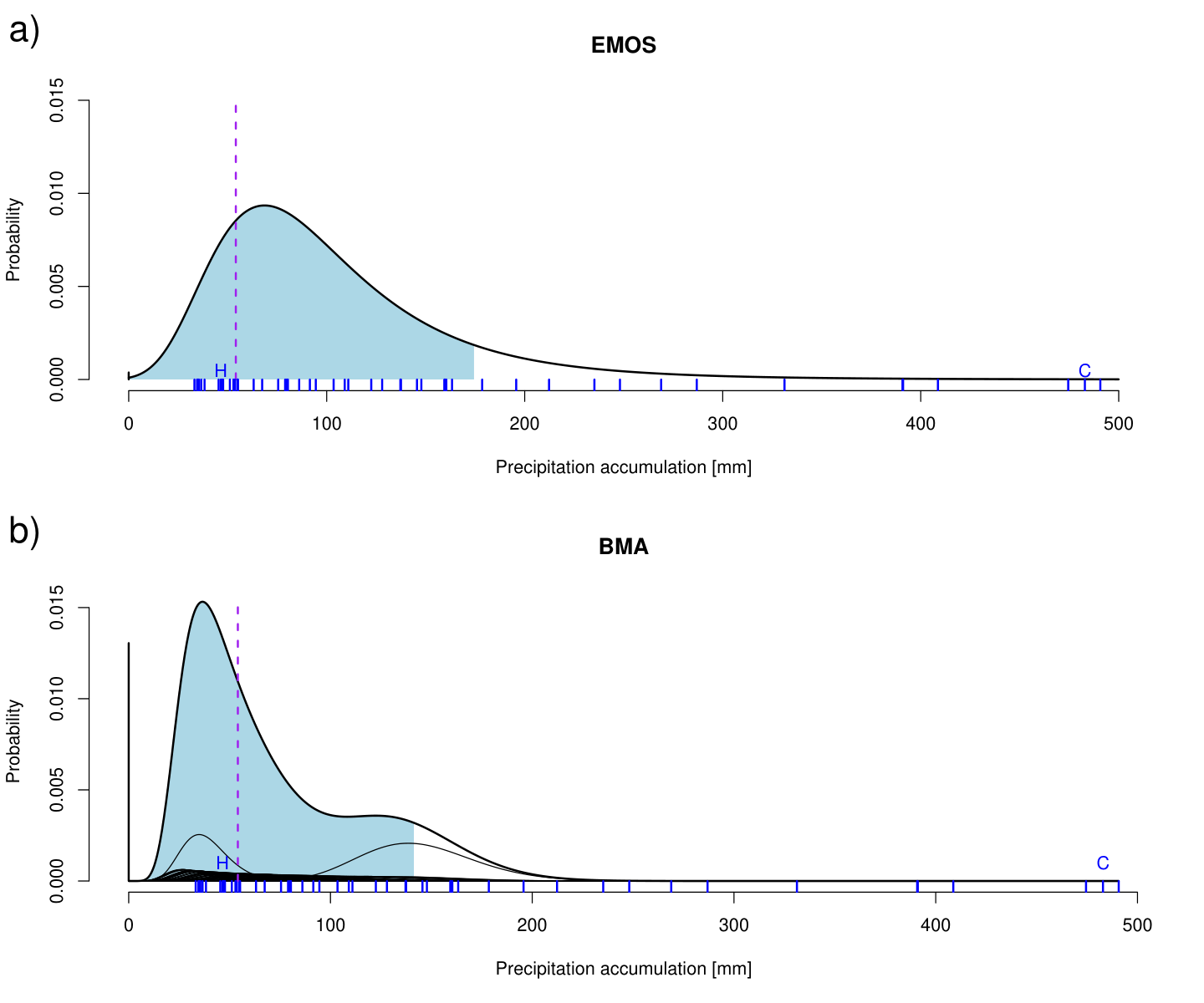
For illustration, Fig. 3a shows an EMOS postprocessed forecast distribution for 5-day accumulated precipitation at Ougadougou, Burkina Faso. The 52 raw ECMWF ensemble members are represented by blue marks; they include eleven values in excess of 200 mm, with the CNT member being close to 500 mm. The ensemble forecast at hand informs the statistical parameters of the EMOS postprocessed forecast distribution, which includes a tiny point mass at zero, and a censored GEV density for positive precipitation accumulations, with the 90th percentile being at 174 mm.
3.4.2 Bayesian Model Averaging (BMA)
A BMA predictive distribution is a weighted sum of component distributions, each of which depends on a single ensemble member. For the ECMWF ensemble, the BMA method for precipitation accumulation proposed and studied by Sloughter et al. (2007) and Fraley et al. (2010) implies a statistical model of the form
with nonnegative weights , , and that sum to 1, and reflect the members’ performance in the training period. The component distributions , , and include a point mass at zero and a density for positive accumulations. The point mass at zero specifies the probability of no precipitation in a logistic regression model, with the cube root of the member forecast and an indicator of it being zero, being linear predictors. The specification for positive amounts derives from a Gamma density for the cube root transformed precipitation accumulation, with a mean that is affine in the cube root transformed ensemble member, and a variance that is an affine function of the member value. While the statistical coefficients for the Gamma mean model are estimated for , , and separately, the coefficients for the Gamma variance model are shared.
Figure 3b shows a BMA postprocessed forecast distribution for the aforementioned forecast case at Ougadougou, Burkina Faso. The postprocessed distribution involves a point mass of about 0.01 at zero, and a mixture of power transformed Gamma densities for positive accumulations, with the 90th percentile being at 141 mm. In this example, the BMA and EMOS postprocessed distributions are sharper than the raw ECMWF ensemble, and nevertheless the verifying accumulation is well captured.
Adaptations to the other ensembles considered in this paper are straightforward as described by Fraley et al. (2010). For example, in the case of the RMM ensemble each of the 15 contributors receive its own component distribution, BMA weight, logistic regression coefficients for the probability of no precipitation, and statistical parameters for the Gamma mean model, whereas the coefficients for the Gamma variance model are shared.
3.4.3 Estimation of statistical parameters
Postprocessing techniques such as EMOS and BMA rely on statistical parameters that need to be estimated from training data, comprising forecast–observation-pairs either from the station or TRMM pixel at hand, or from all stations or applicable TRMM pixels within the considered region, and typically from a rolling training period consisting of the most recent days for which data are available at the initialization time. We employ the regional approach with a rolling training period of days which yields superior results, consistent with the literature (Thorarinsdottir and Gneiting, 2010, e.g., ). The local approach requires longer training periods, and (in experiments not shown here) yields very similar results then.
For EMOS, parameter estimation is based on CRPS minimization over the training data, which is computationally efficient, as closed expressions for the CRPS under GEV distributions are available (Scheuerer, 2014). For BMA, we employ maximum likelihood estimation, implemented via the expectation-maximization (EM) algorithm developed by Sloughter et al. (2007). All computations were performed in R (R Development Core Team, 2017) based on the ensembleBMA package (Fraley et al., 2011) and code supplied by Michael Scheuerer.
4 Results
Our annual evaluation period ranges from 1 May to 15 October, covering the wet period of the West African monsoon. The assessment of ECMWF ensemble forecasts is based on monsoon seasons 2007–2014, and for the other TIGGE sub-ensembles we restrict according to availability as indicated in Table 1.
For verification against station observations, this yields more than 3,000, 6,000, and 12,000 forecast–observations pairs per monsoon season in East Sahel, West Sahel, and Guinea Coast. For verification against TRMM observations, we use 30 randomly chosen, non-overlapping boxes per region at and aggregation, and eight sites per region for longitude–latitude boxes. This covers substantial parts of the study region and results in about 5,000 forecast–observation pairs per monsoon season at the smaller aggregation levels, and well over 1,000 pairs at our highest level.
In subsection 4.1, we study the skill of 1-day accumulated ECMWF raw and postprocessed ensemble precipitation forecasts in detail. Subsections 4.2 and 4.3 present results and highlight differences for longer accumulation times and spatially aggregated forecasts. Subsection 4.4 turns to results for all TIGGE sub-ensembles, and we investigate the gain in predictability through inter-model variability using the RMM ensemble. In our (u)PIT histograms and reliability diagrams, we show results for the last available monsoon season 2014 only, given that operational systems continue to be improving (Hemri et al., 2014).
4.1 1-day accumulated ECMWF forecasts
Figure 4 shows (u)PIT histograms for 1-day accumulated raw and postprocessed ECMWF ensemble and EPC forecasts over West Sahel, East Sahel, and Guinea Coast. The histograms for the raw ensemble indicate strong underdispersion as well as a wet bias (panels a–c). At Guinea Coast, about 56% of the observations are smaller than the smallest ensemble member, a result that is robust across monsoon seasons. EMOS and BMA postprocessed forecasts generally are calibrated (panels g–l), as is EPC (panels d–f). Statistical postprocessing also corrects for the systematically too high PoP values issued by the raw ECMWF ensemble. As shown in Fig. 5, EMOS and BMA postprocessed PoP forecasts are reliable, but are hardly ever higher than 0.70. Generally, the postprocessed PoP forecasts have reliability and resolution similar to EPC.
Table 2 shows the mean Brier score (BS), mean CRPS, and mean absolute error (MAE) for the various forecasts and regions, with the scores being averaged across monsoon seasons 2007–2014. We use a simple procedure to check whether differences in skill are stable across seasons. If a method has higher (worse) mean score than EPC in all eight seasons, we mark the score --; if it is judged worse in seven seasons, we put down a -. Similarly, if a method has smaller (better) mean score than EPC in all seasons, we mark the score ++; if it performs better in seven seasons, we label + in the table. Viewed as a (one-sided) statistical test of the hypothesis of predictive skill equal to EPC, the associated tail probabilities or -values are and respectively. Clearly, the raw ECMWF ensemble underperforms relative to EPC, with -- designations throughout, and the EMOS and BMA postprocessed forecasts perform at about the same level as EPC.
| BS | CRPS | MAE | |||||||
| West | East | Guinea | West | East | Guinea | West | East | Guinea | |
| Sahel | Sahel | Coast | Sahel | Sahel | Coast | Sahel | Sahel | Coast | |
| ENS | --0.32 | --0.32 | --0.48 | --4.50 | --2.63 | --6.99 | --5.36 | --3.13 | --8.39 |
| EPC | 0.19 | 0.15 | 0.23 | 3.75 | 2.08 | 5.28 | 4.60 | 2.38 | 6.57 |
| EMOS | 0.19 | 0.15 | 0.23 | 3.75 | 2.15 | +5.25 | 4.65 | --2.45 | 6.60 |
| BMA | +0.18 | 0.15 | ++0.22 | 3.71 | 2.07 | ++5.20 | 4.58 | 2.38 | 6.53 |
The Murphy diagrams in Fig. 6 corroborate these findings. For 1-day precipitation occurrence, decision makers will mostly prefer the climatological reference EPC over the raw ECMWF ensemble, and only some decision makers will have a slight preference for EMOS or BMA postprocessed forecasts, as compared to EPC. These are sobering results, as they suggest that over northern tropical Africa ECMWF 1-day accumulated precipitation forecasts are hardly of use.
4.2 Longer accumulation times
One might expect NWP precipitation forecasts to improve relative to EPC at longer accumulation times, as the main focus in forecasting shifts from determining time and location of initiation and subsequent propagation of convection towards determining regions with enhanced or reduced activity, based on large-scale conditions. Longer lead times might also lead to growth in differences between perturbed members, and thus reduce raw ensemble underdispersion.
The PIT histogram in of Fig. 7a indicates only slight, if any, improvement in calibration for raw ECMWF 5-day accumulated precipitation forecasts over West Sahel, and the results for the other regions are similar (not shown). Raw ensemble reliability improves at longer accumulation times, verified against either station observations in panel b), or TRMM observations in panels c) and d), though at a loss of resolution.
| BS | CRPS | MAE | |||||||
| West | East | Guinea | West | East | Guinea | West | East | Guinea | |
| Sahel | Sahel | Coast | Sahel | Sahel | Coast | Sahel | Sahel | Coast | |
| ENS | 0.14 | --0.25 | --0.10 | --12.80 | --8.42 | --19.69 | 16.23 | --10.76 | -24.41 |
| EPC | 0.12 | 0.16 | 0.08 | 11.63 | 7.07 | 16.54 | 16.15 | 9.56 | 22.98 |
| EMOS | 0.13 | 0.16 | -0.08 | 11.62 | 7.34 | 16.44 | +15.99 | 9.96 | 22.74 |
| BMA | +0.11 | ++0.15 | 0.08 | ++11.47 | +6.94 | 16.33 | +16.07 | +9.45 | 22.92 |
Table 3 uses the same setting as Table 2, but the scores are now for 5-day accumulated precipitation. The raw ECMWF ensemble still underperforms relative to EPC. The EMOS and BMA postprocessed forecasts outperform EPC only slightly, with the differences in scores being small and typically not being stable across monsoon seasons. Despite the change in the underlying forecast problem, even postprocessed ECMWF ensemble forecasts are generally not superior to EPC.
4.3 Spatially aggregated observations
For the assessment of forecast skill at larger spatial scales, we focus on ECMWF raw and BMA postprocessed ensemble forecasts over West Sahel, evaluated by the Brier score and CRPS. This is due to the similarities in CRPS and MAE results, better performance of
| TRMM 0.25 0.25∘ / 1 d | TRMM 1 1∘ / 1 d | TRMM 52∘ / 1 d | ||||||||||
| BS | CRPS | CRPS | CRPS | |||||||||
| West | East | Guinea | West | East | Guinea | West | East | Guinea | West | East | Guinea | |
| Sahel | Sahel | Coast | Sahel | Sahel | Coast | Sahel | Sahel | Coast | Sahel | Sahel | Coast | |
| ENS | --0.30 | --0.23 | --0.48 | --2.29 | --1.44 | --4.03 | --2.24 | --1.56 | --4.43 | --1.95 | --1.53 | --4.22 |
| EPC | 0.19 | 0.14 | 0.23 | 1.07 | 0.57 | 1.35 | 0.94 | 0.58 | 1.36 | 0.81 | 0.49 | 1.07 |
| BMA | ++0.17 | ++0.13 | ++0.21 | ++1.03 | ++0.55 | ++1.29 | ++0.89 | ++0.55 | ++1.28 | ++0.76 | ++0.45 | ++0.95 |
BMA compared to EMOS in many instances, and results for West Sahel that are as good for BMA postprocessed forecasts as for East Sahel, and better than for Guinea Coast.
The use of spatially aggregated TRMM observations avoids problems of point to pixel comparisons, and at higher aggregation we can assess forecast quality with minimal propagation error. The dry bias of TRMM disadvantages the raw ensemble compared to EPC and postprocessed forecasts, but does not hinder assessments regarding systematic forecast errors. As illustrated in Fig. 7c, 1-day PoP forecasts from the raw ECMWF ensemble remain unreliable even at the gridbox scale. It is only under large scales and longer accumulation times simultaneously, when precipitation occurs almost invariably, that raw ensemble PoP forecasts become reliable (panel d).
Table 4 shows mean Brier and CRPS scores at various spatial aggregations for 1-day precipitation accumulation, verified against TRMM observations. The raw ECMWF ensemble forecast is inferior to EPC at all resolutions, and in every single region and season. BMA postprocessed forecasts outperform EPC across aggregation scales, and in every single region and season, but the improvement relative to EPC remains small.
4.4 TIGGE sub-ensembles and RMM ensemble
In addition to the ECMWF EPS, which we have studied thus far, the TIGGE database contains several more operational sub-ensembles, as listed in Table 1. Figure 8 shows PIT histograms for the various sub-ensembles and the reduced multi-model (RMM) ensemble for 1-day accumulated precipitation forecasts over West Sahel. All TIGGE sub-ensembles exhibit underdispersion and wet biases, though in strongly varying degrees.
Figure 9 displays Brier and CRPS skill scores relative to EPC for raw and BMA postprocessed TIGGE sub-ensemble and RMM ensemble forecasts in 2007–2014, verified against station observations. All raw ensembles underperform relative to EPC, in part drastically so. For most sub-ensembles, a temporal improvement in skill is visible, with monsoon seasons 2011–2014 revealing higher skill than 2007–2010. Postprocessing by BMA increases forecast quality. The ECMWF, KMA, NCEP, and UKMO ensembles yield the best postprocessed forecasts, exhibiting small positive skill relative to EPC for most monsoon periods. The BMA postprocessed RMM ensemble outperforms all sub-ensembles as well as EPC, but the improvement is small. As shown in Fig. 10, the mean perturbed forecasts from the ECMWF, UKMO, and NCEP ensembles are the top three contributors to the BMA postprocessed RMM forecast.
In further experiments, we have studied raw and postprocessed TIGGE sub-ensemble and RMM ensemble forecasts at accumulation times up to 5 days and spatial aggregations up to gridboxes in TRMM. Our findings generally remain unchanged. The raw ensemble forecasts never reaches the quality of the climatological reference EPC. After postprocessing with BMA, the ECMWF ensemble typically becomes the best performing TIGGE sub-ensemble, showing slightly better scores than EPC when verified against TRMM observations, at all spatial aggregations. The BMA postprocessed RMM forecast depends heavily on the ECMWF mean perturbed forecast, and is superior to both EPC and the BMA postprocessed sub-ensemble.
5 Discussion
In a first-ever thorough verification study, the quality of operational ensemble precipitation forecasts from different NWP centers was assessed over northern tropical Africa for several years, accumulation periods, and for station and spatially aggregated satellite observations. All raw ensembles exhibit calibration problems in form of underdispersion and biases, and are unreliable at high PoP forecast values. They have lower skill than the climatological reference EPC for the prediction of occurrence and amount of precipitation, with the underperformance being stable across monsoon seasons.
After correcting for systematic errors in the raw ensemble through statistical postprocessing, the ensemble forecasts become reliable and calibrated, but only few are slightly superior to EPC. Not surprisingly, forecast skill tends to be highest for long accumulation times and large spatial aggregations. Overall, raw ensemble forecasts are of no use for the prediction of precipitation over northern tropical Africa, and even EMOS and BMA postprocessed forecasts have little added value compared to EPC.
What are the reasons for this rather disappointing performance of state-of-the-art global EPSs? For 1-day accumulated precipitation forecasts, the ability of an NWP model to resolve the details of convective organization is essential. As all global EPSs use parameterized convection, this clearly limits forecast skill. The fact that even postprocessed 1-day accumulated ensemble forecasts exhibit no skill relative to EPC, implies that ensembles cannot translate information on the current atmospheric state (e.g., tropical waves or influences from the extratropics) into meaningful impacts regarding the occurrence or amount of precipitation. This is robust for verification against station as well as satellite observations, and can therefore not be explained by propagation errors.
For longer accumulation times and larger spatial aggregations, the large-scale circulation has a much stronger impact on convective activity, which should weaken the limitation through convective parameterization. The skill of 5-day accumulated precipitation forecasts, however, increases only slightly, if at all, compared to 1-day accumulated forecasts. The most likely reason for this is that squall lines have feedbacks on the large-scale circulation, which are not realistically represented in global NWP models either. Marsham et al. (2013) find that the large-scale monsoon state in (more realistic) simulations with explicit convection differs quite pronouncedly from runs with parameterized convection, even when using the same resolution of 12 km. In the explicit-convection simulation, greater latent and radiative heating to the north weakens the monsoon flow, delays the diurnal cycle, and convective cold pools provide an essential component to the monsoon flux. We suspect that some or all of these effects are misrepresented in global EPS forecasts.
The fact that EPS precipitation forecasts are so poor over northern tropical Africa is a strong demonstration of the complexity of the underlying forecast problem. An interesting question in this context is whether poor predictability in the Tropics is unique to northern Africa with its strongly organized, weakly synoptically forced rainfall systems.
Furthermore, the lack of skill motivates alternative approaches to predicting precipitation over this region. Little et al. (2009) compare operational NCEP ensemble, climatological, and statistical forecasts for stations in the Thames Valley, United Kingdom. They note that NCEP forecasts outperform climatological forecasts, but demonstrate that statistical forecasts, solely based on past observations, can outperform NCEP forecasts by exploiting spatio-temporal dependencies. These also exist over northern tropical Africa and some additional predictability may stem from large-scale drivers such as convectively-coupled waves. Fink and Reiner (2003) note a coupling of the initiation of squall lines to African easterly waves and Wheeler and Kiladis (1999) the influence of large-scale tropical waves, such as Kelvin and equatorial Rossby waves or the Madden-Julian oscillation, on convective activity. Pohl et al. (2009) confirm the relation between the Madden-Julian oscillation and rainfall over West Africa and Vizy and Cook (2014) demonstrate an impact of potential extratropical wave trains on Sahelian rainfall. Statistical models based on spatio-temporal characteristics of rainfall and extended by such large-scale predictors seem a promising approach to improve precipitation forecasts over our study region, and we expect such forecasts to outperform climatology. This approach will be explored in future work.
Alternatively, ensembles of convection-permitting NWP model runs, ideally in combination with ensemble data assimilation, could be used, but the computational costs are high, and it will take time until a multi-year database will become available for validation studies. Given the growing socio-economic impact of rainfall in northern tropical Africa with its rain-fed agriculture, statistical and statistical-dynamical approaches should be fostered in parallel in order to improve the predictability of rainfall in this region.
Acknowledgments
The research leading to these results has been accomplished within project C2 “Prediction of wet and dry periods of the West African Monsoon” of the Transregional Collaborative Research Center SFB / TRR 165 “Waves to Weather” funded by the German Science Foundation (DFG). Tilmann Gneiting is grateful for support by the Klaus Tschira Foundation. The authors also thank various colleagues and weather services that have over the years contributed to the enrichment of the KASS-D database; special thanks go to Robert Redl for creating the underlying software. Alexander Jordan and Michael Scheuerer have kindly provided R code, and we are grateful to Sebastian Lerch for constructive suggestions.
Appendix
Rainfall exhibits extremely high spatial and temporal variability, which hinders automated quality checks applicable to other meteorological variables such as temperature or pressure. For precipitation, Fiebrich and Crawford (2001) note only a range and a step test. The global range of station observed 1-day accumulated precipitation is from 0 mm to 1,825 mm. All KASS-D observations passed this test. The step test checks if the difference of neighboring 5-minute accumulated precipitation is smaller than 25 mm. For 1-day accumulated precipitation tests of this type are not meaningful, nor are the persistence tests used by Pinson and Hagedorn (2012) for wind speed.
However, the site-specific climatological distributions of precipitation accumulation should be right-skewed, i.e., the median should be smaller than the mean, and in the Tropics they should have a point mass at zero (Rodwell et al., 2010). As noted, we only consider stations with more than 80% available observations in any of the monsoon seasons, and all 132 stations thus selected passed these tests.
References
- Bougeault et al. (2010) Bougeault, P., and Coauthors, 2010: The THORPEX interactive grand global ensemble. Bulletin of the American Meteorological Society, 91 (8), 1059–1072.
- Brier (1950) Brier, G. W., 1950: Verification of forecasts expressed in terms of probability. Monthly Weather Review, 78 (1), 1–3.
- Buizza et al. (2005) Buizza, R., P. L. Houtekamer, Z. Toth, G. Pellerin, M. Wei, and Y. Zhu, 2005: A comparison of the ECMWF, MSC, and NCEP global ensemble prediction systems. Monthly Weather Review, 133, 1076–1097.
- Davis et al. (2013) Davis, J., P. Knippertz, and A. H. Fink, 2013: The predictability of precipitation episodes during the West African dry season. Quarterly Journal of the Royal Meteorological Society, 139 (673), 1047–1058.
- Ehm et al. (2016) Ehm, W., T. Gneiting, A. Jordan, and F. Krüger, 2016: Of quantiles and expectiles: Consistent scoring functions, Choquet representations and forecast rankings. Journal of the Royal Statistical Society Series B, 78 (3), 505–562.
- Engel et al. (2017) Engel, T., A. H. Fink, and P. Knippertz, 2017: Extreme flooding in the West African cities of Dakar and Ouagadougou — Atmospheric dynamics and implications for flood risk assessments. Journal of Hydrometeorology, submitted.
- Fiebrich and Crawford (2001) Fiebrich, C. A., and K. C. Crawford, 2001: The impact of unique meteorological phenomena detected by the Oklahoma Mesonet and ARS Micronet on automated quality control. Bulletin of the American Meteorological Society, 82 (10), 2173–2187.
- Fink and Reiner (2003) Fink, A. H., and A. Reiner, 2003: Spatiotemporal variability of the relation between African easterly waves and West African squall lines in 1998 and 1999. Journal of Geophysical Research, 108 (D11), 1–17.
- Fink et al. (2006) Fink, A. H., D. G. Vincent, and V. Ermert, 2006: Rainfall types in the West African Sudanian zone during the summer monsoon 2002. Monthly Weather Review, 134 (8), 2143–2164.
- Fink et al. (2011) Fink, A. H., and Coauthors, 2011: Operational meteorology in West Africa: Observational networks, weather analysis and forecasting. Atmospheric Science Letters, 12 (1), 135–141.
- Fink et al. (2017) Fink, A. H., and Coauthors, 2017: Mean climate and seasonal cycle. Meteorology of Tropical West Africa: The Forecasters’ Handbook, D. J. Parker, and M. Diop-Kane, Eds., Wiley-Blackwell, Chichester, chap. 1, 1–39.
- Fraley et al. (2010) Fraley, C., A. E. Raftery, and T. Gneiting, 2010: Calibrating multimodel forecast ensembles with exchangeable and missing members using Bayesian model averaging. Monthly Weather Review, 138 (1), 190–202.
- Fraley et al. (2011) Fraley, C., A. E. Raftery, T. Gneiting, J. M. Sloughter, and V. Berrocal, 2011: Probabilistic weather forecasting in R. The R Journal, 3 (1), 55–63.
- Gneiting (2011) Gneiting, T., 2011: Making and evaluating point forecasts. Journal of the American Statistical Association, 106 (494), 746–762.
- Gneiting (2014) Gneiting, T., 2014: Calibration of Medium-Range Weather Forecasts. Technical Memorandum 719, European Centre for Medium-Range Weather Forecasts.
- Gneiting et al. (2007) Gneiting, T., F. Balabdaoui, and A. E. Raftery, 2007: Probabilistic forecasts, calibration and sharpness. Journal of the Royal Statistical Society Series B, 69 (2), 243–268.
- Gneiting and Raftery (2005) Gneiting, T., and A. E. Raftery, 2005: Weather forecasting with ensemble methods. Science, 310, 248–249.
- Gneiting and Raftery (2007) Gneiting, T., and A. E. Raftery, 2007: Strictly proper scoring rules, prediction, and estimation. Journal of the American Statistical Association, 102 (477), 359–378.
- Gneiting et al. (2005) Gneiting, T., A. E. Raftery, A. H. Westveld, and T. Goldman, 2005: Calibrated probabilistic forecasting using ensemble model output statistics and minimum CRPS estimation. Monthly Weather Review, 133, 1098–1118.
- Hagedorn et al. (2012) Hagedorn, R., R. Buizza, T. M. Hamill, M. Leutbecher, and T. N. Palmer, 2012: Comparing TIGGE multimodel forecasts with reforecast-calibrated ECMWF ensemble forecasts. Quarterly Journal of the Royal Meteorological Society, 138, 1814–1827.
- Haiden et al. (2012) Haiden, T., M. J. Rodwell, D. S. Richardson, A. Okagaki, T. Robinson, and T. Hewson, 2012: Intercomparison of global model precipitation forecast skill in 2010/11 using the SEEPS score. Monthly Weather Review, 140 (8), 2720–2733.
- Hamill (2001) Hamill, T. M., 2001: Interpretation of rank histograms for verifying ensemble forecasts. Monthly Weather Review, 129 (3), 550–560.
- Hamill and Juras (2006) Hamill, T. M., and J. Juras, 2006: Measuring forecast skill: Is it real skill or is it the varying climatology? Quarterly Journal of the Royal Meteorological Society, 132 (621), 2905–2923.
- Hamill et al. (2004) Hamill, T. M., J. S. Whitaker, and X. Wei, 2004: Ensemble reforecasting: Improving medium-range forecast skill using retrospective forecasts. Bulletin of the American Meteorological Society, 132, 1434–1447.
- Hemri et al. (2014) Hemri, S., M. Scheuerer, F. Pappenberger, K. Bogner, and T. Haiden, 2014: Trends in the predictive performance of raw ensemble weather forecasts. Geophysical Research Letters, 41, 9197–9205.
- Houze et al. (2015) Houze, R. A., K. L. Rasmussen, M. D. Zuluaga, and S. R. Brodzik, 2015: The variable nature of convection in the tropics and subtropics: A legacy of 16 years of the Tropical Rainfall Measuring Mission satellite. Reviews of Geophysics, 53 (3), 994–1021.
- Huffman et al. (2007) Huffman, G. J., and Coauthors, 2007: The TRMM multisatellite precipitation analysis (TMPA): Quasi-global, multiyear, combined-sensor precipitation estimates at fine scales. Journal of Hydrometeorology, 8, 38–55.
- Lafore et al. (2017) Lafore, J. P., and Coauthors, 2017: Deep convection. Meteorology of Tropical West Africa: The Forecasters’ Handbook, D. J. Parker, and M. Diop-Kane, Eds., Wiley-Blackwell, Chichester, chap. 3, 90–129.
- Leutbecher and Palmer (2008) Leutbecher, M., and T. N. Palmer, 2008: Ensemble forecasting. Journal of Computational Physics, 227 (7), 3515–3539.
- Little et al. (2009) Little, M. A., P. E. McSharry, and J. W. Taylor, 2009: Generalized linear models for site-specific density forecasting of UK daily rainfall. Monthly Weather Review, 137, 1029–1045.
- Maggioni et al. (2016) Maggioni, V., P. C. Meyers, and M. D. Robinson, 2016: A review of merged high-resolution satellite precipitation product accuracy during the Tropical Rainfall Measuring Mission (TRMM) era. Journal of Hydrometeorology, 17, 1101–1117.
- Marsham et al. (2013) Marsham, J. H., N. S. Dixon, L. Garcia-Carreras, G. M. S. Lister, D. J. Parker, P. Knippertz, and C. E. Birch, 2013: The role of moist convection in the West African monsoon system: Insights from continental-scale convection-permitting simulations. Geophysical Research Letters, 40 (9), 1843–1849.
- Mathon et al. (2002) Mathon, V., H. Laurent, and T. Lebel, 2002: Mesoscale convective system rainfall in the Sahel. Journal of Applied Meteorology, 41 (11), 1081–1092.
- Molteni et al. (1996) Molteni, F., R. Buizza, T. N. Palmer, and T. Petroliagis, 1996: The ECMWF ensemble prediction system: Methodology and validation. Quarterly Journal of the Royal Meteorological Society, 122, 73–119.
- Palmer (2002) Palmer, T. N., 2002: The economic value of ensemble forecasts as a tool for risk assessment: From days to decades. Quarterly Journal of the Royal Meteorological Society, 128, 747–774.
- Park et al. (2008) Park, Y. Y., R. Buizza, and M. Leutbecher, 2008: TIGGE: Preliminary results on comparing and combining ensembles. Quarterly Journal of the Royal Meteorological Society, 134, 2029–2050.
- Parker et al. (2008) Parker, D. J., and Coauthors, 2008: The AMMA radiosonde program and its implications for the future of atmospheric monitoring over Africa. Bulletin of the American Meteorological Society, 89 (7), 1015–1027.
- Pinson and Hagedorn (2012) Pinson, P., and R. Hagedorn, 2012: Verification of the ECMWF ensemble forecasts of wind speed against analyses and observations. Meteorological Applications, 19, 484–500.
- Pohl et al. (2009) Pohl, B., S. Janicot, B. Fontaine, and R. Marteau, 2009: Implication of the Madden–Julian oscillation in the 40-day variability of the West African monsoon. Journal of Climate, 22 (13), 3769–3785.
- R Development Core Team (2017) R Development Core Team, 2017: R: A Language and Environment for Statistical Computing. Vienna, Austria, R Foundation for Statistical Computing, URL http://www.R-project.org.
- Raftery et al. (2005) Raftery, A. E., T. Gneiting, F. Balabdaoui, and M. Polakowski, 2005: Using Bayesian model averaging to calibrate forecast ensembles. Monthly Weather Review, 133, 1155–1174.
- Roca et al. (2010) Roca, R., P. Chambon, I. Jobard, P. E. Kirstetter, M. Gosset, and J. C. Bergés, 2010: Comparing satellite and surface rainfall products over West Africa at meteorologically relevant scales during the AMMA campaign using error estimates. Journal of Applied Meteorology and Climatology, 49, 715–731.
- Rodwell et al. (2010) Rodwell, M. J., D. S. Richardson, T. D. Hewson, and T. Haiden, 2010: A new equitable score suitable for verifying precipitation in numerical weather prediction. Quarterly Journal of the Royal Meteorological Society, 136 (650), 1344–1363.
- Schefzik et al. (2013) Schefzik, R., T. L. Thorarinsdottir, and T. Gneiting, 2013: Uncertainty quantification in complex simulation models using ensemble copula coupling. Statistical Science, 28 (4), 616–640.
- Scheuerer (2014) Scheuerer, M., 2014: Probabilistic quantitative precipitation forecasting using ensemble model output statistics. Quarterly Journal of the Royal Meteorological Society, 140, 1086–1096.
- Sloughter et al. (2007) Sloughter, J. M., A. E. Raftery, T. Gneiting, and C. Fraley, 2007: Probabilistic quantitative precipitation forecasting using Bayesian model averaging. Monthly Weather Review, 135, 3209–3220.
- Söhne et al. (2008) Söhne, N., J.-P. Chaboureau, and F. Guichard, 2008: Verification of cloud cover forecast with satellite observation over West Africa. Monthly Weather Review, 136 (11), 4421–4434.
- Swinbank et al. (2016) Swinbank, R., and Coauthors, 2016: The TIGGE project and its achievements. Bulletin of the American Meteorological Society, 97 (1), 49–67.
- Thorarinsdottir and Gneiting (2010) Thorarinsdottir, T. L., and T. Gneiting, 2010: Probabilistic forecasts of wind speed: ensemble model output statistics by using heteroscedastic censored regression. Journal of the Royal Statistical Society: Series A (Statistics in Society), 173 (2), 371–388.
- van der Linden et al. (2017) van der Linden, R., A. H. Fink, J. G. Pinto, and T. Phan-Van, 2017: The dynamics of an extreme precipitation event in northeastern Vietnam in 2015 and its predictability in the ECMWF ensemble prediction system. Weather and Forecasting, 32 (3), 1041–1056.
- Vizy and Cook (2014) Vizy, E. K., and K. H. Cook, 2014: Impact of cold air surges on rainfall variability in the Sahel and wet African tropics: a multi-scale analysis. Climate Dynamics, 43 (3-4), 1057–1081.
- Wheeler and Kiladis (1999) Wheeler, M., and G. N. Kiladis, 1999: Convectively coupled equatorial waves: Analysis of clouds and temperature in the wavenumber–frequency domain. Journal of the Atmospheric Sciences, 56, 374–399.
- Wilks (2009) Wilks, D. S., 2009: Extending logistic regression to provide full-probability-distribution MOS forecasts. Meteorological Applications, 16, 361–368.
- Wilks (2011) Wilks, D. S., 2011: Statistical Methods in the Atmospheric Sciences. 3rd ed., Academic Press.