NCTS-PH/1719
The Importance of Quantum Pressure of Fuzzy Dark Matter on Lyman-Alpha Forest
Abstract
With recent Lyman-alpha forest data from BOSS and XQ-100, some studies suggested that the lower mass limit on the fuzzy dark matter (FDM) particles is lifted up to . However, such a limit was obtained by CDM simulations with the FDM initial condition and the quantum pressure (QP) was not taken into account which could have generated non-trivial effects in large scales structures. We investigate the QP effects in cosmological simulations systematically, and find that the QP leads to further suppression of the matter power spectrum at small scales, as well as the halo mass function in the low mass end. We estimate the suppressing effect of QP in the 1D flux power spectrum of Lyman-alpha forest and compare it with data from BOSS and XQ-100. The rough uncertainties of thermal gas properties in the flux power spectrum model calculation were discussed. We conclude that more systematic studies, especially with QP taken into account, are necessary to constrain FDM particle mass using Lyman-alpha forest.
pacs
95.35.+dI Introduction
Dark matter is one of the intriguing mysteries of modern cosmology. Currently, the leading paradigm of dark matter is the cold dark matter (CDM), supported by the majority of the observations like the mass-to-light ratio of clusters of galaxies [1], the rotation curves of galaxies [2], the Bullet Cluster [3], the cosmic microwave background (CMB) [4] and the large scale structure of the universe [5]. Despite its success on large scales, the CDM paradigm faces three problems on small scales, dubbed as the “small scales crisis” [6]: (i) the missing satellite problem, (ii) the cusp-core problem, and (iii) the too-big-to-fail problem. The essence of these problems is that CDM predicts an excess amount of dark matter on small scales, and hence the key to address them is to smooth out the small-scale structures by astrophysical processes [7], or invoke alternative dark matter models like warm dark matter (WDM) [8], self-interacting dark matter [9] and fuzzy dark matter (FDM) [10].
The FDM paradigm, in which the dark matter is made of ultra-light bosons in Bose-Einstein condensate state, is an ideal alternative of CDM, since it suppresses small-scale structures while inherits the success of CDM on large scales [11, 12, 13]. For the detailed history and implementation of FDM, one can see Ref. [14] and the reference therein. The suppression effect, arising from the effective “quantum pressure” (QP) of FDM, is directly connected to the mass of the ultra-light axion. The predictions of FDM with mass are consistent with observations of the CMB and large scales structure [15], high- galaxies and CMB optical depth [16], and the density profiles of dwarf spheroidal galaxies [17]. However, recent results claimed that FDM with mass below has already been ruled out at confidence level by comparing the results of hydrodynamic simulations to the Lyman-alpha forest data [18, 19, 20].
Lyman-alpha forest, a series of absorption lines in the Lyman emission spectrum from distant galaxies and quasars by neutral hydrogen (HI) gas at different redshift, provides the information about the the spatial distribution of HI gas at high redshift. In the leading theory of Lyman-alpha forest — the gravitational confinement model — HI clumps are confined by the gravity provided by dark matter halos [21, 22]. Thus, the flux power spectrum of Lyman-alpha forest is a biased representation of the underling DM density field power spectrum [23, 24, 25]. Recently, two collaborations, the Baryon Oscillation Spectroscopic Survey (BOSS) [26] and XQ-100 [27], have announced their analyses between redshift for the flux power spectrum, thus providing tools to constraint dark matter models on an unprecedented high level of precision.
To robustly exclude such a mass range, two tasks have to be carried out before the experimental data analysis. The first is numerical simulations of the FDM system on large scales, which have been performed in a number of approaches: directly solving the Schrödinger-Poission system [17], Smoothed Particle Hydrodynamic (SPH) simulation [28], and N-body simulation with Particle-Mesh (PM) method [29]. However, all these simulations were restricted in simulation scale and suffered from the singularity problem at zero-density points in the calculation of QP. In this paper, we adopt an independent simulation scheme developed in Ref. [30], which provides DM-only simulations with SPH and particle-particle (PP) interactions to account for QP, is feasible for implementation in cosmological scale simulations, and avoids the singularity problem.
The second is the uncertainties in hydrodynamic simulations. In the N-body simulation, the uncertainty in the matter power spectrum is originating from the use of different initial conditions, the adoption of different orders of Lagrangian perturbation theory [31], finite-box effect [32] and the usage of different N-body simulation codes [33, 34, 35]. These uncertainties can be precisely estimated and controlled because their properties are well studied. In contrast, the uncertainties from hydrodynamic simulations can be of orders of magnitude [36, 37, 34, 35]. Different treatments introduced in hydrodynamic simulations in handling the gaseous part induce huge discrepancy in gas density, gas temperature and galaxy structure. Moreover, different hydrodynamic simulation codes contribute uncertainties to the 1D flux power spectrum at the level of . As stated in Ref. [38], several additional astrophysical processes may also alter the 1D flux power spectrum, such as patchy reionization and smoothing.
We estimate the constraint on the mass range of FDM from Lyman-alpha forest data with DM-only cosmological simulations in four different settings: (1) standard CDM simulation, (2) simulation using FDM-modified initial condition and CDM dynamics, (3) simulation using FDM-modified initial condition and dynamics with FDM mass equals to , (4) . By utilizing the 1D flux power spectrum of the CDM hydrodynamic simulation in Ref. [18], one can obtain the 1D flux power spectrum for the corresponding condition using the 3D power spectrum ratio from our simulations.
Our results are shown in the aspects of density field, halo mass function, 3D power spectrum and 1D flux power spectrum with Lyman-alpha forest data. We show that the effect of QP in structure formation is non-trivial and introduce important suppression in the growth of structures. Inspired by the linear theory summarized in Ref. [39], we have calculated the uncertainty range of the 1D flux power spectrum based on the unknown hydrogen gas temperature properties. The suppression of the 1D flux power spectrum from higher gas temperature behaves like the suppression caused by FDM.
This paper is arranged as follows. In Sec. II, we discuss the methodology of the simulation, simulation set-up and initial conditions. We also review the linear theory of 1D flux power spectrum calculation. In Sec. III, we present our results in the aspects of density field, halo mass function, 3D power spectrum and 1D flux power spectrum. We compare our 1D flux power spectrum to the Lyman-alpha forest data. In Sec. IV, we discuss the gas temperature uncertainty. Finally, we summarize our outcomes in Sec. V.
II Methodology
II.1 Quantum Pressure as particle-particle interaction
Standard N-body simulations have problems in calculating the QP because of the discretization of the density field by the delta function. From the expression of QP, obviously, what we need in the calculation is a smooth density field. There are already some reliable smoothing particle methods used in the N-body simulation of the FDM system with limited box sizes (), e.g., Ref. [28, 29]. For the sake of Lyman forest, it is important to have a cosmological scale simulation so that the study of structure formation and matter power spectrum on large scales is possible.
We proposed a novel N-body simulation scheme for FDM in a previous work [30], in which the delta function is replaced by a smooth Gaussian kernel function to solve the singularity problem and avoid the simulation crash. This scheme can be used to perform simulations at scales no smaller than as we shall prove later and give a coarse-grained description on small scales. However, the original scheme requires some modifications for cosmological simulations. In this section, we will demonstrate how to embed QP in the cosmological simulations.
For cosmological simulations, one has to consider the transformation from physical to comoving coordinates. Under the transformation described in Appendix A, there is an additional pre-factor for the original QP defined in Ref. [30], where is the cosmological scale factor. The QP for a cosmological simulation becomes
| (1) |
, where , , and are the reduced Planck constant, FDM particle mass and the mass density of FDM, respectively. The corresponding acceleration can be written as
| (2) |
where , , , and are the mass of the simulation particle, a normalization factor accounting for the volume occupied by simulation particles, the de Broglie wavelength of FDM particles, and the correction factor for high-density regions, respectively. For more detailed explanations of , please refer to Appendix A of Ref. [30].
To demonstrate the effect of QP, we consider a two-particle system separated by a distance of order , and the acceleration caused by QP will be . In Fig. 1, the QP effect is presented in the plane of (, ). The acceleration from QP, gravity, and their sum are shown by the black dashed line, blue solid line, and red solid line, respectively. Apparently, the effect of QP is attractive if the separation between the two particles is shorter than , otherwise repulsive. To understand this phenomenon, we refer back to the definition of QP in Eq. (1): is proportional to the curvature of the density, which can be negative, positive, or zero, physically corresponding to negative, positive, and zero forces, respectively. The reason of the difference between Fig. 1 here and the Fig. 1 of [30] is that the mass of the simulation particle is changed from to . The effect of gravity is directly related to the mass of the simulation particles while the QP is not affected due to the fact that the normalization factor in Eq. (2) is chosen to be the same as the mass of the simulation particles. In other words, the strength of QP is a quantity independent of the simulation particle mass . Therefore, the acceleration of gravity is considerably larger in a cosmological simulation due to the larger mass of the simulation particles. Thus, the structure formation in large scales is still dominated by gravity. However, the QP plays a non-trivial role in the structure formation, particularly in highly non-linear regions such as dark matter halos.
II.2 Simulation settings
We use the code Gadget2 [40], which is a TreePM hybrid N-body code, to perform our simulations. To describe QP, we discretize the interaction term and modify Gadget211 1 The code is called Axion-Gadget, publicly available at https://github.com/liambx/Axion-Gadget to calculate QP in the same way as in Ref. [30]. (The PM method is helpful for cosmological simulations with periodic boundary conditions.) Because QP behaves like a short-range force, we adopt the original PM code to compute the long-range force and modify the Tree code which takes care of the short-range force to include the calculation of QP. In addition, it is not necessary to set softening length for QP since QP is finite in the region.
We start our simulation from the redshift . The related cosmological parameters are DM energy density , cosmological constant , baryon energy density , dimensionless Hubble parameter , scalar spectral index , and the power spectrum normalization factor .
We generated the initial CDM power spectrum following Ref. [42]. The suppression of the FDM power spectrum relative to the CDM one on small scales can be characterized by a transfer function [41]
| (3) |
where is the wavenumber and and are the three-dimensional power spectra of FDM and CDM, respectively. One has to bear in mind that the physical difference between and 22 2 The transfer functions and are defined in Eq. (1) of Ref. [42], which transfer the power spectrum at large scales () to the power spectrum at other scales () for the corresponding model. Restricted to linear theory, the current matter power spectrum would be proportional to the product of the primordial power spectrum given by inflation theory and embodying the growth of structure, . At the super-horizon scale, cosmological perturbation theory shows that the structure does not grow, and hence the transfer function is set with boundary condition . is characterized by the transfer function , which transforms the power spectrum from CDM to FDM and so is deduced as the ratio of FDM transfer function to CDM transfer function .
Following the arguments in Ref. [43], we can well approximate by the redshift-independent expression [10]
| (4) |
The parameter is the critical scale of Jeans wavenumber at matter-radiation equality. In Fig. 2, we present the square of the transfer function with three different FDM masses to demonstrate the suppression of FDM power spectrum in small scales relative to CDM power spectrum. The blue, black, and red solid lines correspond to the masses of the FDM being , , , respectively. The vertical green dashed line represents the Nyquist limit which is the resolution limit of our simulations and the corresponding wavenumber is computed to be
where is the volume of the simulation box, and is the total number of simulation particles, which are and respectively in our simulations. The origin of this limit is due to the fact that each simulation particle has an approximate average volume and we cannot know what happens inside the simulation particle. In other words, the result is not reliable for . One can see that there is a sharp break of FDM power spectrum at and severe oscillations occur with suppression for for all three different FDM masses. For a smaller mass, the suppression is tremendous compared to a larger mass which behaves almost the same as the CDM case at high .
We modify the code 2LPTic [44] for generating the initial conditions of the CDM power spectrum for cosmological simulations to incorporate the transfer function so as to generate initial conditions with the FDM power spectrum.
II.3 1D Flux Power Spectrum
The calculation of the 1D flux power spectrum in the linear regime is well summarized in Ref. [39],
| (5) | |||||
| (6) |
First, the linear dark matter power spectrum was calculated by CAMB [45], with the same parameters used in the simulations. Then we calculate the baryon power spectrum from Eq. (5), in which is the Jeans wavenumber related to the Jeans length by
| (7) |
Finally, we integrate Eq. (6) to get the one-dimensional flux power spectrum, in which we need the bias function
| (8) |
Here
is a parameter related to the velocity dispersion of the HI gas at redshift , and is the average temperature of HI gas at redshift . is the polytropic index in the equation of state of HI gas 33 3 For an ideal polytropic gas, the temperature at redshift and position is . is a normalizing factor, whose effect is the same as the parameter in .
For further calculation, we use a power-law parametrization of and
| (9) |
where the 1 uncertainty ranges are
| (10) |
These are copied from the Table. II in Ref. [46]. As for and , we treat them as redshift independent constants with the 1 uncertainty ranges as in Ref. [4, 47]
| (11) |
The formulae discussed above are only applicable to linear perturbation, and the insertion of non-linear matter power spectrum in Eq. (6) is problematic. However, for the sake of simplicity, the 1D flux power spectrum is assumed to be related to the DM density power spectrum with the following equation,
| (12) |
which is inspired by the linear theory. Here represents the bias introduced by the thermal properties of intergalatic medium (IGM), but the distortions in the direction of line-of-sight is neglected. Given the form of Eq. (12), the 1D flux power spectrum is the 3D matter power spectrum convolved with the bias along the line of sight. On one hand, we assume that the dynamics of dark matter does not affect the gaseous component, and the bias is the same in all four different simulations. On the other hand, we reweigh the matter power spectrum with the 3D matter power spectrum ratio of the simulations FDM/FIC/F23 to the simulation CDM. That is to say, we first take the derivative of the 1D flux power spectrum , from the mock 1D flux power spectrum in hydrodynamic simulation shown in Ref. [48], with respect to
| (13) |
and multiply the right hand side (RHS) of this equation by the ratio , where FDM, FIC and F23. Then we integrate this expression to get the modified 1D flux power spectrum
| (14) |
By comparing the modified and the original , we can tell the effect of FDM model on Lyman alpha forest.
III Numerical result
| Abbreviations | Initial Conditions | Dynamics | FDM mass |
|---|---|---|---|
| CDM | CDM-Standard | CDM-Standard | — |
| FIC | FDM-modified | CDM-Standard | |
| FDM | FDM-modified | FDM-modified | |
| F23 | FDM-modified | FDM-modified |
We have performed four different kinds of simulations for comparison as listed in Table. 1. To avoid words cluttering in the following presentation, we use abbreviations for these four simulations. In this section, we first present the density field of the simulation FDM as well as the density field difference between the simulations FDM and FIC. We then compare the 3D power spectra and 1D flux power spectra of all four simulations in order to investigate the non-linear effect of the QP. After showing the 1D flux power spectrum, a numerical chi-square test of Lyman-alpha forest data from BOSS and XQ-100 is performed. Finally, we discuss the constraint on the FDM mass.
III.1 Density Field and Halo Mass Function

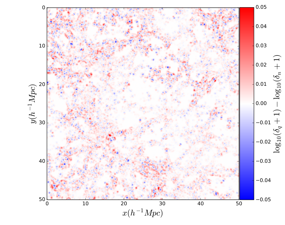
In the left panel of Fig. 3, we depict the density field taken from a slice of the simulation cube. The slice is thick, and the density field is calculated from the particle distribution by the triangular shaped cloud (TSC) scheme but further smoothed by a Gaussian filter (variance ) for better illustration. With the color scale, one can clearly see that the large scales structures include voids, filaments and knots. The density contrast is defined as
where the subscript denotes that it is from the simulation FDM. The color scale of Fig. 3 represents the logarithm of , which is the ratio of local density to the average density . In the right panel of Fig. 3, we compare the density field of the simulation FDM and the simulation FIC. The color scale shows the difference between the logarithm of and the logarithm of .
We found that the difference between the density fields of the two simulations FDM and FIC is small, but the effect of QP can produce granular structures close to the high density regions. Note that these granular structures are indeed due to QP, but not the difference in the initial conditions by comparing the density fields of the simulations FIC and CDM.


To illustrate more details in small scale, we select a Mpc sub-box projected in y direction and zoom in for better resolution. In Fig. 4, the left panel is from the simulation FDM and the right panel is from the simulation FIC. The density field is calculated from the particle distribution by the nearest grid point scheme and further smoothed by bilinear algorithm. We note that the cluster in the simulation FDM looks much fuzzier than the one in the simulation FIC. Qualitatively, the formation of low mass halos is further suppressed when taking QP into consideration.
We identified the halos using the package AHF [49], which can build up the hierarchical structure for the halos and sub-halos in the snapshots of our simulations. The halos are identified if the average density of the halo is over 200 times the critical density of the universe. In Fig. 5, the halo mass function is presented with the FDM mass . The colors represent different redshifts, and the solid, dot-dashed and dashed lines represent the halo mass function of the simulations CDM, FIC and FDM, respectively. The break of the halo mass functions at (the green dashed line) is due to our limited resolution. By definition, we cannot identify halos whose mass is below . From halo masses to , there is no recognizable difference among the simulations FDM, FIC and CDM. However, for halo mass below , the difference becomes noticeable.
To quantitatively see the difference, one can refer to the right panel of Fig. 5 which manifestly demonstrates the suppression caused by the QP and the modified initial condition. We can see that QP (FDM simulation) introduces more suppression on the number density of halos than that of FIC simulation, with modified initial condition only. There is no identifiable effect in the simulations FDM and FIC for the halo mass function with .
It is clear that the difference in modified initial conditions and QP start to have significant influence on the formation of halos. Furthermore, it is worth mentioning that by using the code established in Ref. [30] we are able to explore halo mass smaller than in cosmological simulations.
III.2 Impacts on Lyman-Alpha Forest
Here we investigate the difference in the 1D flux power spectrum among our four simulations with the method mentioned in Sec.II.3, which enables us to quantitatively study the effect of the modified initial condition and dynamics introduced by FDM. Furthermore, our result of 1D flux power spectrum will be used to compare with the BOSS/XQ-100 data.
In Fig. 6, we compare the 3D power spectra at different redshifts among different simulations CDM, FIC, FDM and F23. In the left panel of Fig. 6, the effect of FDM initial condition is almost negligible at low redshifts but plays an important role at high redshifts. However, the effect of QP is non-negligible even at low redshifts. During the non-linear gravitational evolution even without the QP, the power spectrum of the simulation FIC grows differently from the simulation CDM. However, at the power spectra of the simulations FIC and CDM almost overlap, and one can barely see the difference between them. The effect of the FDM initial condition turns out to be a tiny suppression on power spectrum at low redshifts.
On the other hand, the power spectrum of the simulation FDM is clearly different from the simulations FIC and CDM at low redshifts because of the non-trivial QP effect. For the power spectrum of the simulation F23, the suppression on small scales is even more significant than all other simulations due to its larger QP.
In the right panel of Fig. 6, we show the ratio of the 3D power spectra from the simulations FDM, FIC and F23 to that of simulation CDM. One can see that the QP suppresses the power spectrum by relative to the simulation FIC at for three different redshifts . However, for , the 3D power spectra from the simulations FDM, FIC and F23 are identical. Therefore, we can conclude that, QP has no effect on large scale, which is well-expected. For , since it is approaching our resolution limit, the results should be taken carefully and critically. The effect of QP in the simulation F23 is clearly more significant than the simulation FDM.
The 1D flux power spectra are shown in the left panel of Fig. 7 for comparison with the data of BOSS and XQ-100 at three different redshifts . The solid, dot-dashed, dashed and dotted lines represent 1D flux power spectra from the simulations CDM, FIC, FDM and F23, respectively. The dots and error bars are the data from BOSS in darker colors and XQ-100 in lighter colors. At the small-scale region , which corresponds to in the discussion of the matter power spectrum, the 1D flux power spectra for the simulations FDM and F23 are relatively more suppressed than those of CDM and FIC. Although the simulation FIC differs from CDM in the initial condition, the difference in their spectra is still small.
The right panel of Fig. 7 shows the ratio of the 1D flux power spectra of the simulations FIC, FDM and F23 to that of the simulation CDM. The degree of suppression is up to at for the simulation FDM. Additionally, the 1D flux power spectrum of the simulation F23 is suppressed even more than the simulation FDM. On the contrary, the degree of suppression is smaller than at for the simulation FIC. For , the difference in the 1D flux power spectra for the simulations FDM, FIC and CDM is less than . In fact, the QP contribution cannot be neglected even if the QP is sub-dominant as shown in Fig. 1.
Finally, it is clear that a full investigation of hydrodynamic simulations with the QP is necessary to robustly constrain the mass region of FDM.
IV Discussion
It has been reported in Ref. [19, 18, 20] that the FDM mass can be excluded up to at significance. However, the systematic uncertainties arising from both simulation (N-body and hydrodynamics) and gas properties (like the temperature of gas) were not discussed adequately in these works.
Note that the well-known discrepancies in simulation will introduce uncertainties on the observables, e.g. the code-to-code inconsistency in hydrodynamic simulations introduces at least uncertainty in 1D flux power spectrum as shown in Ref. [50, 51]. A brief discussion of the uncertainties in simulation is given in Appendix B for interested readers.
In the previous section, we consider the effects of FDM. However, the thermal properties of IGM also impact the 1D flux power spectrum, as shown in Eq. (6) and Eq. (12). Since these two effects are degenerate in the linear power spectrum, one should consider them simultaneously before reaching any conclusion. In this subsection, we will discuss the possible uncertainty caused by the gas temperature and compare it with that cause by FDM mass to see their degeneracy in the power spectrum.
First, as an illustration of the potential effects of gas, we consider the prediction of the linear theory and its uncertainty. There are several parameters in Eq. (6), but for simplicity we only consider the uncertainty of FDM particle mass and average gas temperature . The error of the 1D flux power spectrum can be expressed as
| (15) |
We apply this formula to the linear 1D power spectrum at redshift and set , in the calculation of partial derivatives. For the most optimistic estimation, we set , so that we can express in terms of . In a most conservative precision , one can obtain a maximum temperature uncertainty and compare it to the current uncertainty of . From Eq. (10), the best-fit and 1 uncertainty of at redshift is about
For FDM mass , is larger than . Therefore we can actually exclude this kind of FDM model robustly with Lyman-alpha observation. However, for FDM mass in the range from to , we need much higher precision of the temperature to draw the conclusion (see Table. 2).
Second, we use a similar method as in Sec. III.2, with one difference in the RHS of Eq. (13); we multiply the ratio of bias function with different gas temperature rather than the ratio of matter power spectra,
| (16) |
Here we used the Bias function in the linear theory Eq. (8). Even though at the redshift range to , the structure in the universe is non-linear, we still use the ratio predicted by linear theory because our purpose here is to demonstrate the uncertainty of gas temperature instead of studying the thermal properties of gas which requires full hydrodynamics simulation.
As in Sec. III.2, we will calculate the ratio again and compare it with the suppression induced by FDM. The best-fit value is calculated from Eq. (9) with and . The upper limit in the red shaded region in Fig. 8 is given by and while the lower limit corresponds to and , which are chosen according to the 1 uncertainty Eq. (10). From Fig. 8, it is obvious that the current constraint on the temperature of gas is not good enough to exclude FDM mass , let alone the fact that we have not even included the uncertainties of other thermal parameters of the gas. A detailed study of the thermal properties of the gas is needed to settle the issue.
Finally, as Hui et al. pointed out in Ref. [38], several additional astrophysical processes may also alter the 1D flux power spectrum, such as the effects of fluctuations in the ionizing background [38], patchy reionization [52], modification of the thermal history [53], and galactic outflows [54]. These additional factors are yet absent in many of the present cosmological simulations. To sum up, the uncertainties from both numerical and physical factors prevent us from constraining the mass of FDM precisely, unless models and analyses with percent level precisions are available. A hydrodynamic simulation handling all of the uncertainties is needed in the future to set the correct constraint on the FDM mass.
V Conclusion
In this paper, we have extended our FDM smoothed-particle hydrodynamics methodology to cosmological N-body simulation. Unlike previous works in literature, we have implemented not only the FDM initial condition but also the QP effect to our cosmological N-body simulations. The correct transformation of QP from physical to comoving coordinates has been derived in this work. With this new technique, we have performed four different simulations, CDM, FIC, FDM, and F23. We have shown the difference of over-density between FIC and FDM simulations. We have found that some granular structures located at higher density regions can be produced by QP. Remarkably, we are able to probe halos with mass smaller than in cosmological simulations based on our methodology.
The matter power spectra from our four simulations tell us that the impact from QP is non-trivial, as shown by the difference between FIC and FDM. Comparing with CDM in the region with wavenumber Mpc, the power spectrum suppression due to the effect of initial condition is less than at redshift , but the QP effect can cause suppression in the same region. Hence, the impact from QP on the power spectrum is more significant than that from initial conditions at low redshifts. Moreover, the QP effect also depends on the redshift. At high redshifts the effect of modified initial condition is more important than QP, but vice versa at low redshifts . Considering the DM mass around , the matter power spectrum of the simulation F23 shows a large deviation from that of CDM in the wavenumber region.
Using the results of these four different simulations, we then further studied the flux power spectrum of Lyman-alpha forest. We obtain the 1D flux power spectrum by integrating the 3D matter power spectrum taken from our simulation result. There is still suppression on the flux power spectra of FDM and F23 on small scales compared to that of CDM. However, the difference between FIC and CDM is small, which indicates that the suppression due to the transfer function of FDM is consumed by the non-linear evolution. To summarize, by comparing the flux power spectra of different simulations, we demonstrate that the QP causes non-trivial effect on small scales, which could be important in the study of Lyman-alpha forest.
Finally, we discussed the uncertainties in simulations and models. As an example, we did a rough estimation and found that the average gas temperature and FDM mass are degenerate since a smaller or a higher both suppress the 1D flux power spectrum. We found that the current constraint on the average temperature of the gas is not accurate enough to exclude FDM mass , which is summarized in Table. 2 and Fig. 8.
We conclude that the QP plays an important role in structure formation and affects the prediction for Lyman-alpha forest significantly. A further comprehensive hydrodynamic simulation including the QP and a precise constraint on the gas temperature of Lyman-alpha forest are needed to solidly set a lower bound on the FDM particle mass.
Acknowledgment
We would like to acknowledge Eric Armengaud and Vid Iršič for discussion and Lachlan Lancaster for useful suggestions. We also would like to acknowledge Lam Hui and Tom Broadhust for useful comments. This work is partially supported by a CUHK Discretionary Fund and by the MoST of Taiwan under the grant no.: 105-2112-M-007-028-MY3.
Appendix A detail of the comoving transformation
We show the full transformation of the QP from physical to comoving coordinates. The Lagrangian can be expressed as
| (17) |
where , , , , and are mass and velocity of simulation particles, mass of FDM, density in physical coordinate, average density in physical coordinate and gravitational potential, respectively. The first, second and the third terms in Eq. (17) are the kinetic energy, the potential energy arising from the QP and the gravitational potential energy, respectively. We follow the basic transformations
| (18) |
which incorporate the scale factor to account for the expansion of the universe. Here denotes the physical coordinates and denotes the comoving coordinates.
After including the transformations, the Lagrangian Eq. (17) becomes
| (19) |
where we define
| (20) |
The transformation of the Poisson equation can be written as
| (21) |
where is the density of the cosmological constant. In order to simplify the equation, we perform a canonical transformation on the Lagrangian
| (22) |
which does not change the equation of motion. Now the Lagrangian can be written as
| (23) |
where we define for simplicity. Consequently, the Poisson equation is converted to
| (24) |
From the second equation of the Friedmann equations,
| (25) |
one can obtain
| (26) |
Additionally, we define and acquire . Now the Lagrangian can be written as
| (27) |
Hence we can define the canonical momentum as
| (28) |
and write down the Hamiltonian
| (29) |
As a consequence, we obtain the equations of motion
| (30) |
In the equations of motion, the terms for gravity and QP have prefactors and respectively, and hence we need to treat them separately in the comoving coordinates. In the physical coordinates, we can deal with these two terms simultaneously since .
Appendix B simulation uncertainty
The systematic uncertainties in N-body simulation are well studied. The matter power spectrum is affected by the methodology of generating initial condition for simulations, such as the choice between the first order Lagrangian perturbation theory (1LPT) and the second order Lagrangian perturbation theory (2LPT) can introduces difference in the matter power spectrum, as reported in Ref. [31]. The halo mass function in the large mass end is sensitive at level to the choice of the finite simulation box size, which can be corrected owing to their clear nature [32].
The uncertainty resulting from different N-body simulation codes is numerically hard to estimate, and the origin of the discrepancies among different codes is also barely known. Such kind of issues are comprehensively discussed in Ref. [33]. Roughly speaking, the discrepancy between different codes is within in the matter power spectrum and halo mass function. However, Ref. [34, 35] reported a discrepancy in the center and in the outskirts of the halo by comparing the halo density profile from several different codes.
Unlike the errors in the N-body simulations, the uncertainties involved in hydrodynamic simulations are much larger. Usually, a considerable uncertainty can be introduced due to the treatments of the gaseous component. As demonstrated in Ref. [36, 37, 34, 35], a large inconsistency of the galaxy structure can be caused by using different hydrodynamic codes. Quantitatively, the errors of the gas density and temperature in the centers of the galaxies are about one to two orders of magnitude, estimated by comparing different hydrodynamic codes.
The one-dimension (1D) flux power spectrum of Lyman alpha forest can also contain some level of uncertainties, e.g., see the code comparison in Ref. [50, 51]. For hydrodynamic simulations using ENZO [55] and using Gadget2, there is also a difference in the 1D flux power spectrum and difference in the probability distribution of density and temperature. Moreover, for simulations using AREPO [56] and Gadget2, there are also difference in their 1D flux power spectra.
References
- [1] N. A. Bahcall, L. M. Lubin, and V. Dorman, The Astrophysical Journal Letters 447, L81 (1995), astro-ph/9506041.
- [2] J. Einasto, A. Kaasik, and E. Saar, Nature 250, 309 (1974).
- [3] D. Clowe et al., The Astrophysical Journal Letters 648, L109 (2006), astro-ph/0608407.
- [4] P. Ade et al., Astronomy & Astrophysics 594, A13 (2016), 1502.01589.
- [5] M. Tegmark et al., The Astrophysical Journal 606, 702 (2004), astro-ph/0310725.
- [6] D. H. Weinberg, J. S. Bullock, F. Governato, R. K. de Naray, and A. H. Peter, Proceedings of the National Academy of Sciences 112, 12249 (2015), 1306.0913.
- [7] A. Pontzen and F. Governato, Nature 506, 171 (2014), 1402.1764.
- [8] P. Colin, V. Avila-Reese, and O. Valenzuela, The Astrophysical Journal 542, 622 (2000).
- [9] D. N. Spergel and P. J. Steinhardt, Physical Review Letters 84, 3760 (2000), astro-ph/9909386.
- [10] W. Hu, R. Barkana, and A. Gruzinov, Physical Review Letters 85, 1158 (2000), astro-ph/0003365.
- [11] D. J. Marsh, Physics Reports 643, 1 (2016), 1510.07633.
- [12] X. Du, C. Behrens, and J. C. Niemeyer, Monthly Notices of the Royal Astronomical Society 465, 941 (2017), 1608.02575.
- [13] P. Mocz et al., (2017), 1705.05845.
- [14] J.-W. Lee, (2017), 1704.05057.
- [15] R. Hlozek, D. Grin, D. J. Marsh, and P. G. Ferreira, Physical Review D 91, 103512 (2015), 1410.2896.
- [16] B. Bozek, D. J. Marsh, J. Silk, and R. F. Wyse, Monthly Notices of the Royal Astronomical Society 450, 209 (2015), 1409.3544.
- [17] H.-Y. Schive, T. Chiueh, and T. Broadhurst, Nature Physics 10, 496 (2014), 1406.6586.
- [18] V. Iršič, M. Viel, M. G. Haehnelt, J. S. Bolton, and G. D. Becker, arXiv preprint arXiv:1703.04683 (2017).
- [19] E. Armengaud, N. Palanque-Delabrouille, C. Yèche, D. J. Marsh, and J. Baur, arXiv preprint arXiv:1703.09126 (2017).
- [20] T. Kobayashi, R. Murgia, A. De Simone, V. Iršič, and M. Viel, ArXiv e-prints (2017), 1708.00015.
- [21] M. Rees et al., Monthly Notices of the Royal Astronomical Society 218, 25P (1986).
- [22] S. Ikeuchi, Astrophysics and space science 118, 509 (1986).
- [23] D. H. Weinberg, R. Dav’e, N. Katz, and J. A. Kollmeier, arXiv preprint astro-ph/0301186 (2003).
- [24] A. Arinyo-i Prats, J. Miralda-Escudé, M. Viel, and R. Cen, Journal of Cosmology and Astroparticle Physics 2015, 017 (2015).
- [25] M. Viel, M. G. Haehnelt, and V. Springel, Mon. Not. Roy. Astron. Soc. 354, 684 (2004), astro-ph/0404600.
- [26] N. Palanque-Delabrouille et al., Astron. Astrophys. 559, A85 (2013), 1306.5896.
- [27] S. López et al., Astron. Astrophys. 594, A91 (2016), 1607.08776.
- [28] P. Mocz and S. Succi, Physical Review E 91, 053304 (2015), 1503.03869.
- [29] J. Veltmaat and J. C. Niemeyer, arXiv preprint arXiv:1608.00802 (2016).
- [30] J. Zhang, Y.-L. S. Tsai, K. Cheung, and M.-C. Chu, arXiv preprint arXiv:1611.00892 (2016).
- [31] B. LHuillier, C. Park, and J. Kim, New Astronomy 30, 79 (2014).
- [32] J. Bagla and J. Prasad, Monthly Notices of the Royal Astronomical Society 370, 993 (2006).
- [33] K. Heitmann, M. White, C. Wagner, S. Habib, and D. Higdon, The Astrophysical Journal 715, 104 (2010).
- [34] J.-h. Kim et al., The Astrophysical Journal Supplement Series 210, 14 (2013).
- [35] F. Sembolini et al., Monthly Notices of the Royal Astronomical Society 457, 4063 (2016).
- [36] B. W. Oshea, K. Nagamine, V. Springel, L. Hernquist, and M. L. Norman, The Astrophysical Journal Supplement Series 160, 1 (2005).
- [37] F. Vazza et al., Monthly Notices of the Royal Astronomical Society 418, 960 (2011).
- [38] L. Hui, J. P. Ostriker, S. Tremaine, and E. Witten, Phys. Rev. D95, 043541 (2017), 1610.08297.
- [39] H. Mo, F. Van den Bosch, and S. White, Galaxy formation and evolution (Cambridge University Press, 2010).
- [40] V. Springel, Monthly Notices of the Royal Astronomical Society 364, 1105 (2005).
- [41] W. Hu, R. Barkana, and A. Gruzinov, Phys. Rev. Lett. 85, 1158 (2000), astro-ph/0003365.
- [42] D. J. Eisenstein and W. Hu, The Astrophysical Journal 496, 605 (1998), astro-ph/9709112.
- [43] H.-Y. Schive, T. Chiueh, T. Broadhurst, and K.-W. Huang, Astrophys. J. 818, 89 (2016), 1508.04621.
- [44] M. Crocce, S. Pueblas, and R. Scoccimarro, Astrophysics Source Code Library 1, 01005 (2012).
- [45] A. Lewis and A. Challinor, Astrophysics Source Code Library (2011).
- [46] M. Viel, G. D. Becker, J. S. Bolton, and M. G. Haehnelt, Physical Review D 88, 043502 (2013).
- [47] A. Rorai et al., Science 356, 418 (2017).
- [48] V. Iršič et al., Mon. Not. Roy. Astron. Soc. 466, 4332 (2017), 1702.01761.
- [49] S. R. Knollmann and A. Knebe, Astrophys. J. Suppl. 182, 608 (2009), 0904.3662.
- [50] J. A. Regan, M. G. Haehnelt, and M. Viel, Monthly Notices of the Royal Astronomical Society 374, 196 (2007).
- [51] S. Bird et al., Monthly Notices of the Royal Astronomical Society , sts590 (2013).
- [52] R. Cen, P. McDonald, H. Trac, and A. Loeb, Astrophys. J. 706, L164 (2009), 0907.0735.
- [53] A. Garzilli, A. Boyarsky, and O. Ruchayskiy, (2015), 1510.07006.
- [54] M. Viel, J. Schaye, and C. M. Booth, Mon. Not. Roy. Astron. Soc. 429, 1734 (2013), 1207.6567.
- [55] G. L. Bryan et al., The Astrophysical Journal Supplement Series 211, 19 (2014).
- [56] V. Springel, Proceedings of the International Astronomical Union 6, 203 (2010).