Optimization of Heterogeneous Coded Caching

Alexander Michael Daniel Wei Yu ^†^†thanks: Manuscript prepared on August 24, 2026. This work is supported by Natural Science and Engineering Research Council (NSERC). The authors are with the Edward S. Rogers Sr. Department of Electrical and Computer Engineering, University of Toronto, Toronto, ON M5S 3G4, Canada (e-mails: alex.daniel@mail.utoronto.ca, weiyu@ece.utoronto.ca).

Abstract

This paper aims to provide an optimization framework for coded caching that accounts for various heterogeneous aspects of practical systems. An optimization theoretic perspective on the seminal work on the fundamental limits of caching by Maddah Ali and Niesen is first developed, whereas it is proved that the coded caching scheme presented in that work is the optimal scheme among a large, non-trivial family of possible caching schemes. The optimization framework is then used to develop a coded caching scheme capable of handling simultaneous non-uniform file length, non-uniform file popularity, and non-uniform user cache size. Although the resulting full optimization problem scales exponentially with the problem size, this paper shows that tractable simplifications of the problem that scale as a polynomial function of the problem size can still perform well compared to the original problem. By considering these heterogeneities both individually and in conjunction with one another, insights into their interactions and influence on optimal cache content are obtained.

Index Terms:

Coded caching, linear programming, non-uniform popularity, non-uniform cache size, non-uniform file length

I Introduction

I-A Background

Caching technologies stand poised to make an important contribution to future 5G cellular networks [1]. One such technique is coded caching, which, roughly speaking, is the idea of using carefully designed user cache content to enable content delivery via coded multicast transmissions. (The cached contents themselves are uncoded.) First introduced by Maddah-Ali and Niesen in [2, 3], coded caching has since been the subject of a great number of studies seeking to extend the original scheme into more practical scenarios. The coded caching scheme of [2, 3] is developed for a system in which a central server has complete knowledge of user numbers and identities, users have identical cache sizes and make a single download request, transmission occurs over an error free link, and files are of equal length and popularity. Subsequent work has since extended the coded caching idea to the decentralized system [4], and to systems with non-uniform file popularity [5, 6, 7, 8, 9, 10, 11, 12, 13, 14, 15, 16, 17], non-uniform file length [18, 19], multiple user requests [20, 21, 22, 23], non-uniform cache size [24, 25, 26, 27], and non-uniform channel quality [28, 29, 30, 31, 32, 33, 34, 35, 36, 37, 38, 39, 40].

The aforementioned works typically either discuss how the scheme of [2, 3] should be modified to accommodate the considered heterogeneity, or develop an entirely new scheme that enables coded multicast transmissions while accommodating the aforementioned heterogeneity. Most of these papers, however, consider only one type of non-uniformity. While this is sensible from the viewpoint of understanding how each heterogeneity affects coded caching systems by itself, practical systems would have to account multiple types of non-uniform parameters. Moreover, we cannot in general expect the effects of these non-uniformities to be additive. It is thus important to consider combinations of heterogeneities, which, to the best of our knowledge, only a few recent works have started to explore: the recent work [19] examines the achievable rate region for a system serving two users with two files, where the user cache sizes and file lengths are not necessarily uniform, while some of the aforementioned work on caching with non-uniform channel quality exploits heterogeneous cache size to rectify disparities in channel quality (see e.g. [33] and references therein).

I-B Main Contributions

This paper proposes an optimization theoretic framework to design caching schemes capable of accommodating non-uniform file length, non-uniform file popularity, and non-uniform user cache size at the same time. More specifically, we design a caching scheme that uses a generalized version of the transmission scheme of [4], paired with an optimization problem designed to yield the optimally coded content. This optimization problem, although convex, has the number of variables, constraints, and objective function terms that scale exponentially with the problem size, so subsequently this paper develops high-quality simplifications that scale polynomially with the problem size, yet perform well compared to the original problem. The proposed optimization approach only yields numerical answers corresponding to the optimized caching schemes, but also generate practical insight into the problems considered.

Optimization approaches have been used in the past for content placement for femtocaching systems [41, 42], but its use in the coded caching context has only appeared recently: for instance, [43] uses an information-theory based optimization problem to help characterize the achievable rate region for certain numbers of users and files in the case where all other systems parameters are uniform. More related is the recent work [27] in which an optimization framework similar to the one used here is employed to develop a caching scheme in the case of non-uniform cache size. Crucially, both approaches design cache content in terms of the subsets of users who have cached the content (see Section III). While we directly express our transmission scheme in terms of that cache content, the approach in [27] is to further design two sets of variables through which the transmission scheme is expressed. Moreover, the framework used in [27] does not distinguish between different files beyond designing a scheme for the worst-case scenario where users request different files. This prevents their framework from addressing file heterogeneity, whereas ours allows for it. Finally, while the optimization problem in [27] suffers from the same exponential scaling problem that the general problem here has, they do not present any tractable methods of solution like we do here.

During the preparation of this paper, we became aware of independent work [17], which uses an optimization framework essentially the same as the one proposed here to study the case of non-uniform file popularity. While independently and simultaneously developed, a number of results in [17] are echoed in this paper. Specifically, both works develop the same exponential-order general optimization problem; then a simplified polynomial-order optimization problem is developed for the non-uniform popularity case (Section IV-C of this paper), although the exact formulations are different. Moreover, both works show that in the special case of uniform popularity, the caching and delivery scheme of [2, 3] is the optimal solution (Section III of this paper); however, the proof in [17] is quite involved, while a much simpler proof is presented here. Ultimately, the focus of [17] is to study the case of non-uniform popularity in great depth, while here, it is only considered as an intermediate step towards the study of the interactions of several heterogeneities at the same time. Thus, despite the similarities, both papers develop many unique insights of practical significance. Indeed, the results of [27] and [17] taken jointly with the results of this paper suggest that the optimization framework common to all three works is likely to be a useful one for coded caching.

I-C Notation

The notation $[a:b]$ is used as shorthand for the set of consecutive integers $\{a,a+1,\dots,b-1,b\}$ , and $[b]$ is used as an abbreviation of $[1:b]$ . The symbol $\oplus$ is used to denote the bitwise “XOR” operation between two or more files (i.e. strings of bits). Both $l$ and $W^{(l)}$ are used to refer to the $l$ -th file under consideration. For an arbitrary file $W^{(n)}$ , $|W^{(n)}|$ refers to the length of the file, and $W^{(l)}_{\mathcal{S}}$ , called a “subfile” of file $W^{(l)}$ , refers to the portion of file $l$ stored exclusively on the caches of the users in the set $\mathcal{S}$ . For notational convenience, notation of the form $W^{(l)}_{123}$ is used instead of $W^{(i)}_{\{1,2,3\}}$ (for the $\mathcal{S}=\{1,2,3\}$ case in this example), returning only to the latter notation if necessary to resolve ambiguity. For a set $\mathcal{S}$ , $\mathcal{P}(\mathcal{S})$ refers to the power set of $\mathcal{S}$ . For a real number $t$ , $\lfloor\cdot\rfloor$ and $\lceil\cdot\rceil$ denote the floor and ceiling functions, respectively.

We define the binomial coefficient $\binom{n}{k}$ in the usual way for $0\leq k\leq n$ , i.e. $\binom{n}{k}=n!/(k!(n-k!))$ , but for $n<0$ or $k>n$ , we take $\binom{n}{k}=0$ . Moreover, the notation of the so-called “multinomial coefficient” is used, defined as:

\binom{n}{k_{1},k_{2},\dots,k_{m}}=\frac{n!}{k_{1}!k_{2}!\dots k_{m}!},

where $k_{1}+k_{2}+\dots+k_{m}=n$ . We use the notation $\sum_{i=a}^{b}n_{i}$ in the usual way when $a\leq b$ , and take $\sum_{i=a}^{b}n_{i}=0$ identically if $a>b$ . More generally, a sum over an empty set of indices is taken to equal zero. Finally, if a sum over an empty set is raised to the power of zero, we take the resulting value to be 1; this is simply used for notational convenience.

I-D Organization

The organization of the rest of the paper is as follows. Section II introduces the optimization framework used in this paper and Section III uses this framework to provide a new interpretation and understanding of [2, 3, 4] by showing how they represent feasible points in the optimization problem. Sections IV-VI use the framework to develop tractable simplifications of the original problem for different types and combinations of non-uniformities. Section VII concludes the paper with a summary and discussion of main results.

II Optimization Perspective on Coded Caching

We begin by providing an optimization perspective on the coded caching schemes of Maddah-Ali and Niesen for both the centralized [2, 3] and the decentralized [4] cases. The transmission scenario consists of a server with a set of $N$ files, $\mathcal{F}=\{1,2,\dots,N\}=[N]$ , serving a set of $K$ users, $\mathcal{U}=\{1,2,\dots,K\}=[K]$ , over a shared, error-free link. For full generality, we allow each file $l$ to have a distinct length of $F_{l}$ bits and a distinct probability $p_{l}$ of being requested, and allow each user $k$ to have arbitrary cache size of $M_{k}$ bits.

Central to the coded caching scheme of [2, 3, 4] is the partitioning of each file $l\in\mathcal{F}$ into subfiles $W^{(l)}_{\mathcal{S}}$ , indexed by all subsets of $\mathcal{S}\subseteq\mathcal{U}$ . (No two subfiles have a non-empty intersection; together the subfiles jointly reconstruct the original file.) In the caching phase, each user $k$ caches

\bigcup_{l,\mathcal{S}\in\mathcal{P}(\mathcal{U}\setminus\{k\})}W^{(l)}_{\mathcal{S}\cup k}

(1)

without coding. In the content delivery phase, given the set of user requests $\mathbf{d}=[d_{1},\dots,d_{K}]$ , where $d_{k}$ denotes the index of the file requested by user $k$ , the server transmits

\bigoplus_{k\in\mathcal{S}}W^{(d_{k})}_{\mathcal{S}\setminus\{k\}}

(2)

over the shared link with zero-padding if necessary, for each $\mathcal{S}\in\mathcal{P}(\mathcal{U})\setminus\emptyset$ , so that together with uncoded content stored a priori in each user’s local cache, all users are guaranteed to be able to reconstruct the entirety of their requested files.

Any coded caching scheme (with coded transmission and uncoded cache) can be described using this “subset partitioning” representation [4]. Different caching strategies differ in their partitioning of the subfiles. But instead of thinking of the above as a way of labelling the cache contents, we can also use this to design the cache content, and regard the size of each subfile $W^{(l)}_{\mathcal{S}}$ as design variables. Consequently, instead of designing cache contents by assigning discrete bits to sets, the problem can be simplified by designing only the sizes of the subfiles: if we have $|W^{(l)}_{\emptyset}|=b^{(l)}_{\emptyset},|W^{(l)}_{1}|=b^{(l)}_{1},\dots,|W^{(l)}_{\mathcal{U}}|=b^{(l)}_{\mathcal{U}}$ , then the first $b^{(l)}_{\emptyset}F_{l}$ bits of $W^{(l)}$ are assigned to $W^{(l)}_{\emptyset}$ , the next $b^{(l)}_{1}F_{l}$ bits to $W^{(l)}_{1}$ , and so on, assigning the final $b^{(l)}_{\mathcal{U}}F_{l}$ bits to $W^{(l)}_{\mathcal{U}}$ . (Formally, this requires that $b^{(l)}_{\mathcal{S}}\in\{0,1/F_{l},\dots(F_{l}-1)/F_{l},1\}$ , but for large $F_{l}$ , this can be relaxed to $b^{(l)}_{\mathcal{S}}\in[0,1]$ without any significant loss.)

For example, consider the centralized scenario wherein the numbers and identities of users are known in advance, so the server has the ability to design the cache content of each user. The coded caching scheme of [2, 3] (assuming uniform file length, cache size and uniform popularity) sets $|W_{\mathcal{S}}|$ to be non-zero for only the $\mathcal{S}$ ’s with $|\mathcal{S}|=t=KM/N$ . In the decentralized setting of [4], all subfiles have non-zero sizes due to the use of random cache content. More generally, $|W^{(l)}_{\mathcal{S}}|$ can be explicitly designed.

The design of coded caching in this way imposes some natural constraints on the subfile sizes. First, the subfiles together must contain the entire file, i.e.

\sum_{\mathcal{S}\in\mathcal{P}(\mathcal{U})}|W^{(l)}_{\mathcal{S}}|=F_{l},\;\;\forall l\in\mathcal{F}.

(3)

Second, denoting the amount of cache dedicated to file $l$ by user $k$ as $\mu_{k,l}$ , the amount of a file cached by a user is expressed as

\sum_{\mathcal{S}\in\mathcal{P}(\mathcal{U}\setminus\{k\})}|W^{(l)}_{\mathcal{S}\cup k}|\leq\mu_{k,l},\;\;\forall k\in\mathcal{U},\forall l\in\mathcal{F},

(4)

where

\sum_{l=1}^{N}\mu_{k,l}=M_{k},\forall k\in[K].

(5)

Finally, the subfiles cannot have a negative size:

|W^{(l)}_{\mathcal{S}}|\geq 0,\quad\forall\mathcal{S}\in\mathcal{P}(\mathcal{U}),\quad\forall l\in\mathcal{F}.

(6)

In the transmission defined in (2), zero-padding is neeeded whenever the subfiles do not have the same length, so the length of a single transmission is determined by the largest subfile in the transmission. For a vector of user requests $\mathbf{d}$ , the number of bits sent to satisfy user requests given in $\mathbf{d}$ is thus

R_{\mathbf{d}}=\sum_{\mathcal{S}\in\mathcal{P}(\mathcal{U})\setminus\emptyset}\max_{k\in\mathcal{S}}\left\{|W^{(d_{k})}_{\mathcal{S}\setminus\{k\}}|\right\}

(7)

The set of choices of $|W^{(l)}_{\mathcal{S}}|$ define a broad family of caching schemes. To find the most efficient caching strategy among this family of schemes that minimize the expected delivery rate over all demand requests, we can formulate the following optimization problem:

	minimize	$\displaystyle\mathbb{E}[R_{\mathbf{d}}]=\sum_{\mathbf{d}\in\mathcal{F}^{K}}p(\mathbf{d})\sum_{\mathcal{S}\in\mathcal{P}(\mathcal{U})\setminus\emptyset}\max_{k\in\mathcal{S}}\left\{\|W^{(d_{k})}_{\mathcal{S}\setminus\{k\}}\|\right\}$		(8)
	subject to	(3)-(6).		(9)

We note before continuing that the transmission scheme described above is the same for all possible user requests, which may be suboptimal if there is repetition in the users’ requests, i.e. the same file is requested by more than one user. However, it can readily be shown that the probability of each user requesting a distinct file goes to one as $N\rightarrow\infty$ of a fixed $K$ . Since it is likely that $N\gg K$ in practice, the optimization formulation (8) can be therefore be used without fear of significant loss.

The optimization problem (8)-(9) is convex in the $|W_{\mathcal{S}}|$ variables. However, there are $N2^{K}$ variables, $N^{K}(2^{K}-1)$ summands in the objective function, and $N2^{K}+KN+N+K$ constraints, making it impractical to solve for large-scale problems. The rest of this paper is dedicated to developing simplifications of (8)-(9) that allow for high quality (and even optimal) solution while maintaining a tractable problem size.

III Homogeneous Coded Caching

Consider the special case of problem (8)-(9) with uniform file lengths, $F_{l}=F,\forall l\in[N]$ , uniform file popularities, $p_{l}=1/N,\forall l\in[N]$ , and uniform cache sizes $M_{k}=M,\forall k\in[K]$ ; this is the same system originally considered in [2, 3]. The symmetry of the resulting problem can be exploited to reduce the computational complexity of optimization. Specifically, define $v_{j}$ such that $v_{j}=|W_{\mathcal{S}}|$ for all $\mathcal{S}$ such that $|\mathcal{S}|=j$ and for all files $W$ ; this reduces the number of optimization variables from an exponential number in $K$ to a linear number in $K$ . Since the file length, file popularity and cache size are all homogeneous, there is symmetry across both the users and the files, and so we would expect the solution to (8)-(9) for this uniform case to have this form, i.e., any two subfiles have the same size if their respective user sets are the same size. The summands of the objective function now simplify as

\max_{k\in\mathcal{S}}\left\{|W^{(k)}_{\mathcal{S}\setminus\{k\}}|\right\}=|W^{(k^{\prime})}_{\mathcal{S}\setminus\{k^{\prime}\}}|=v_{|\mathcal{S}|-1}

where $k^{\prime}$ is any user in the set $\mathcal{S}\setminus\{k\}$ , because each subfile in a given transmission is the same size. Since the files are equally popular, every request vector is equally likely, and since every transmission scheme requires the same number of bits to satisfy the requests, the average does not need to be taken across all the $N^{K}$ possible demands as in (8). Finally, since $v_{j}F$ bits are sent to any subset of $j+1$ users, and there are $\binom{K}{j+1}$ subsets of $j+1$ users, the objective function becomes

\mathbb{E}[R_{\mathbf{d}}]=\sum^{K-1}_{j=0}\binom{K}{j+1}v_{j}F,

(10)

Note that the number of terms in the objective function now scales linearly in $K$ instead of exponentially in $K$ , because each term in (10) accounts for a combinatorial number of transmissions.

The constraints simplify as well. Since all files are of equal length, only one file reconstruction constraint is required. Then, because there are $\binom{K}{j}$ subsets of size $j$ , the file reconstruction constraint becomes

\sum_{j=0}^{K}\binom{K}{j}v_{j}=F.

(11)

Moreover, since the cache sizes are uniform, only one cache constraint is needed, and since all file are homogeneous, an equal amount of memory is allocated to each. The cache constraint thus simplifies to

\sum_{j=1}^{K}\binom{K-1}{j-1}v_{j}\leq MF/N,

(12)

because there are $\binom{K-1}{j-1}$ subsets of size $j$ that contain the index $k$ . As a final step, we follow [2, 3] and normalize the file length $F=1$ in (10)-(12). This yields the following linear programming problem with $K+1$ variables, $K+3$ constraints, and $K$ terms in the objective function:

minimize	$\displaystyle\sum^{K-1}_{j=0}\binom{K}{j+1}v_{j}$	(13)
subject to	$\displaystyle\sum_{j=0}^{K}\binom{K}{j}v_{j}=1,$	(14)
	$\displaystyle\sum_{j=1}^{K}\binom{K-1}{j-1}v_{j}\leq M/N,$	(15)
	$\displaystyle v_{j}\geq 0,\;\;\forall j\in\mathcal{U}.$	(16)

Note that the reduction to an optimization problem that scales as a linear function of $K$ and as a constant function of $N$ is possible because of the symmetry created by the uniform file length, file popularity, and cache size. Later in this paper, cases when one or more of these parameters are non-uniform are treated; but the reduction from the exponential order will no longer be without loss of generality.

Note also that the schemes of [2, 3] and [4] are all feasible points of this problem. In particular, assuming that $t=KM/N$ is an integer, the caching scheme of [2, 3] sets $v_{t}=1/\binom{K}{t}$ and $v_{j}=0$ if $j\neq t$ , while the decentralized scheme of [4] sets the variables to be of the form $v_{j}=(M/N)^{j}(1-M/N)^{K-j}$ for all $j$ . For the non-integer $t$ case, a similar scheme is also stated in [2, 3]. The following theorem shows that the caching scheme of [2, 3] is, in fact, the optimal scheme among the broad family of schemes discussed above. The theorem works for the cases of integer or non-integer $t$ . We note that while a similar result for the integer $t$ case exists in [17], the proof used here uses a novel reformulation over the probability simplex. It is considerably simpler and lends additional insight into the problem.

Theorem 1.

Assume $M\leq N$ . The unique, optimal solution to (13)-(16) is:

•

For $t=KM/N\in\mathbb{Z}$ :

$\displaystyle v_{j}^{*}=$ $\displaystyle\begin{cases}1/\binom{K}{t}&\text{if }j=t,\\ 0&\text{if }j\neq t\end{cases}$ (17)

•

For $t=KM/N\notin\mathbb{Z}$ :

\displaystyle v_{j}^{*}=

\displaystyle\begin{cases}s/\binom{K}{\lfloor t\rfloor}&\text{if }j=\lfloor t\rfloor\\ (1-s)/\binom{K}{\lceil t\rceil}&\text{if }j=\lceil t\rceil\\ 0&\text{else}\end{cases}

(18)

where $s=\lceil t\rceil-t$ .

Proof:

First, we make a change of variables: $a_{j}=v_{j}/\binom{K}{j}$ ; after some mild algebra, the original problem (13)-(16) can be reformulated as:

minimize	$\displaystyle\sum^{K}_{j=0}\frac{K-j}{j+1}a_{j}$	(19)
subject to	$\displaystyle\sum_{j=0}^{K}ja_{j}\leq t$	(20)
	$\displaystyle\sum_{j=0}^{K}a_{j}=1$	(21)
	$\displaystyle a_{j}\geq 0,\quad\forall j\in[0:K].$	(22)

In this form, the optimization problem is more easily understood. Constraints (21) and (22) restrict the feasible space to the probability simplex. The key features of the formulation is that the coefficients of the objective function $\frac{K-j}{j+1}$ are decreasing in $j$ with decreasing second differences, while the cache constraint (20) now has coefficients that increase linearly in $j$ . Intuitively, the optimal solution would involve placing as much “probability mass” in high- $j$ $a_{j}$ variables in order to lower the objective function, but not so high as to violate the cache constraint. This results in the optimal $a_{j}$ to concentrate around at most two consecutive $j$ ’s close to $t$ .

To complete the argument, we first observe that at the optimal solution $\mathbf{a}^{*}$ of (19)-(22), the cache constraint (20) must be tight, when $M\leq N$ . This is because if it were not, one can always shift some of the weight of $a_{j}$ to a higher indexed $a_{j+1}$ without violating the constraints while lowering the objective function. In the practical context, this means that the optimal caching strategy does not waste any cache space.

Second, for a similar reason, we can show that if a feasible solution $\mathbf{a}=[a_{0},\dots,a_{K}]^{T}$ to (19)-(22) has two non-zero variables $a_{i_{1}}\neq 0$ and $a_{i_{2}}\neq 0$ such that $i_{2}-i_{1}\geq 2$ , then $\mathbf{a}$ cannot be an optimal solution of (19)-(22). This is because for any such $\bf{a}$ , we can always construct a better feasible solution $\bar{\mathbf{a}}=[\bar{a}_{0},\dots,\bar{a}_{K}]^{T}$ in the following way. For some small $\Delta$ , set $\bar{a}_{i_{1}}=a_{i_{1}}-\Delta$ , $\bar{a}_{i_{1}+1}=a_{i_{1}+1}+\Delta$ , $\bar{a}_{i_{2}}=a_{i_{2}}-\Delta$ , $\bar{a}_{i_{2}-1}=a_{i_{2}-1}+\Delta$ , and $\bar{a}_{j}=a_{j}$ for all other $j$ values. (If $i_{1}+1=i_{2}-1$ , then set $\bar{a}_{i_{2}-1}=a_{i_{2}-1}+2\Delta$ .) Note that such $\bar{\mathbf{a}}$ remains on the probability simplex; the cache constraint remains satisfied as $\sum_{j=0}^{K}j\bar{a}_{j}=\sum_{j=0}^{K}ja_{j}$ , while the objective function decreases strictly, because the coefficients of $a_{j}$ in the objective, $\frac{K-j}{j+1}$ is a decreasing function of $j$ with decreasing second differences.

The above two observations imply that the optimal solution has either only one non-zero variable, or two non-zero variables that have adjacent indices, i.e. some $j$ and $j+1$ . In this case, the constraints for the optimal solution to (19)-(22) reduce to

ja_{j}+(j+1)a_{j+1}=t,

(23)

and

a_{j}+a_{j+1}=1.

(24)

This system of equations has a unique solution. Indeed, due to (24) and the positivity constraints, (23) implies that $t$ must be a convex combination of $j$ and $j+1$ . If $t\notin\mathbb{Z}$ , the only integer possibility for $j$ is $j=\lfloor t\rfloor$ and $j+1=\lceil t\rceil$ ; representing $t=s\lfloor t\rfloor+(1-s)\lceil t\rceil$ for some $s\in(0,1)$ , it becomes clear that the unique solution to (23)-(24) is $a_{j}=s,a_{j+1}=1-s$ for $j=\lfloor t\rfloor$ and $s=\lceil t\rceil-t$ . If $t\in\mathbb{Z}$ , then we can set $j=t$ , then the unique solution to (23)-(24) is $a_{j}=1,a_{j+1}=0$ . Using the change of variables $v_{i}=a_{i}/\binom{K}{i}$ , this gives the optimal solution to (13)-(16) as stated by (17)-(18). ∎

As a final remark for this section, we acknowledge that there exist stronger results about optimal coded caching schemes than Theorem 1 in the literature, for instance, [44] shows that a slightly modified version of the scheme in [2, 3] is the optimal coded caching scheme among all schemes with uncoded cache content using information theoretical upper bounds. The optimization theoretic perspective of this paper is nevertheless worthwhile in that it easily begets extensions to more practical non-uniform scenarios, which is the focus of the rest of this paper.

IV Coded Caching with Heterogeneous Files

We now move onto the coded caching problem with heterogeneous parameters. Although the optimization problem (8)-(9) is already capable of accounting for non-uniform file popularity, file length, and cache size, the problem size scales exponentially in system parameters, hence the optimization problem is intractable for practical system sizes. The main contributions of this and the next section are to develop simplifications to (8)-(9) that reduce the computational complexity of the problem while maintaining high-quality performance. Each non-uniformity is considered both individually and in conjunction with the others in order to gain insight into the interactions of their respective effects. We begin by examining the effect of non-uniform file popularity and non-uniform file length, but for now keep the cache sizes uniform across the users.

The procedure for each case is roughly as follows: first a new set of variables are defined that are intended to capture some structural feature of the problem, e.g. the $v_{j}$ variables of the simplified homogeneous problem (13)-(16). Next, certain conditions, referred to as memory inequality constraints, are imposed on the new variables (see e.g. (35)), which forces feasible solutions to dedicate more cache memory to certain kinds of files, e.g. more popular files. While no a priori justification for the use of these variable and constraints is given, subsequent numerical results justify their use a posteriori.

These memory inequality constraints then allow the simplification of the objective function (8). First, the max function can be eliminated from (8), since the memory inequality constraints are sufficient to determine a priori which subfiles will be the maximum given some request vector $\mathbf{d}$ . This in turn allows the expected rate to computed precisely in terms of the largest file requested, the second largest file requested, and so on, instead of in terms of the $N^{K}$ possible request vectors. Since there are $K$ files requested, and $N$ possibilities for each file, this ultimately reduces the scaling of the objective function from exponential to polynomial, although the objective function does not necessarily scale with $NK$ precisely.

IV-A Prior Work

The effect of non-uniform file popularity, also referred to as non-uniform demands, on coded caching has been explored in a number of papers [5, 6, 7, 8, 9, 10, 11, 12, 13, 14, 15, 16]. In [5, 6], Niesen and Maddah-Ali modify their decentralized scheme from [4] by first grouping users according to the popularity of their respective file requests, and then transmitting to the groups sequentially using the scheme from [4]. The authors of [7, 8, 10, 11, 9] develop an order-optimal scheme using random caching with a graph-based algorithm to design coded multicast transmissions, with [9] focusing specifically on the application of video delivery. In [10, 11], both the popularity of the files and their request correlation are considered when designing the caching and transmission scheme, while in [12, 13, 14, 15], a heterogeneous network structure is considered, with file popularity organized in discrete levels. Using a novel random caching-based scheme, [16] is able to show order-optimality with a constant that is independent of the popularity distribution. Finally, we repeat earlier comments that [17] uses the same optimization framework that is used to study non-uniform popularity in great depth; we nevertheless show our (similar) work for the sake of exposition.

The literature on the effects of non-uniform file length is, however, comparatively scarce. To the best of our knowledge, Zhang et al [18] provide the only scheme designed to accommodate non-uniform file length for a general number of users. A scheme is provided that uses random caching with a transmission scheme similar to the one used in this paper, and upper and lower bounds on system performance are derived. In particular, [18] explores a random caching scheme where files are cached with a probability proportional to size of the file. Non-uniform file size is also explored in the recent letter [19], in which the achievable rate region for both non-uniform file size and non-uniform cache size is characterized, but only for the case of $K=2$ users and $N=2$ files.

Note that it can be argued that if files are indeed different sizes, they can be broken up into smaller packets of a constant size $F^{\prime}$ bits, and then treated as separate files. While this is a reasonable assumption while investigating other aspects of a coded caching scheme, there are two issues that need be addressed in practice. First, if a file is broken up into multiple pieces, then a user who seeks to to download the entire file must make multiple (correlated) requests to the server - a fact that should be accounted for in subsequent system design. The second practical issue comes from the fact that it is unclear how to set the common file size $F^{\prime}$ : efficiency demands that $F^{\prime}$ be as large as possible so that any required headers represent a small proportion of the entire download, while at the same time, $F^{\prime}$ should also be small enough to divide files without significant remainder.

We therefore contend that heterogeneous file length is an important parameter that a practical system must capable of accommodating in one way or another. The approach to handling non-uniform files sizes discussed above may indeed have some merit; some work has been done to analyze the case of multiple requests from users, see e.g. [20, 21, 22, 23], and so an approach based on this technique may be viable. This paper, however, uses a different approach: files are not broken up into smaller files of equal lengths, and so the cache content is designed to accommodate their different lengths. The possibility of comparing the performance of the different approaches is left to future work.

To the best of our knowledge, there has been no work exploring the relationship between file length and popularity and the resulting effect on cache content. In the literature discussed above, it is noted (roughly) that more popular files should be allocated more cache memory, but also that larger files should be allocated more cache memory. Given that, in general, file lengths and popularity may not have any correlation, it is not clear how these non-uniformities jointly affect optimal cache content. These interactions are explored in the following.

IV-B Preliminaries

First, we introduce two lemmas. The first one is a classic result about binomial coefficients, while the second lemma is used to determine the probability that the file $n$ is the $k$ -th largest file requested; the proof of the latter is contained in Appendix -A.

Lemma 1 (Chu-Vandermonde Convolution).

For $N,N_{1},N_{2},$ and $n$ positive integers, with $N_{1}+N_{2}=N$ and $n\leq N$ ,

\binom{N}{n}=\sum_{k=0}^{n}\binom{N_{1}}{k}\binom{N_{2}}{n-k}

(25)

Lemma 2.

Consider $K$ independent multinomial random trials with $N$ possible outcomes per trial, with probabilities $\{p_{1},p_{2},\dots,p_{N}\}$ , denoted by $\mathbf{Z}\in[N]^{K}$ , i.e., $Z_{i}$ , the $i$ -th element of $\mathbf{Z}$ , is the outcome of the $i$ -th trial. Let the random vector ${\bf Y}$ be a sorted version of ${\bf Z}$ , but with index shifted by 1, so that $Y_{0}$ is the smallest element of $\mathbf{Z}$ , $Y_{1}$ is the second smallest element, and so on. The probability mass function of $Y_{m}$ is given by

$\displaystyle\text{Pr}[Y_{0}=i]=$	$\displaystyle\,\,\left(\sum_{l=i}^{N}p_{l}\right)^{K}-\left(\sum_{i+1}^{N}p_{l}\right)^{K},$	(26)
$\displaystyle\text{Pr}[Y_{1}=i]=$	$\displaystyle\,\,\text{Pr}[Y_{0}=i]+K\left(\left(\sum_{l=1}^{i-1}p_{l}\right)\left(\sum_{l=i}^{N}p_{l}\right)^{K-1}\right.$
	$\displaystyle-\,\left.\left(\sum_{l=1}^{i}p_{l}\right)\left(\sum_{l=i+1}^{N}p_{l}\right)^{K-1}\right),$	(27)

and for $m\in[2:K-1]$ ,

	$\displaystyle\text{Pr}[Y_{m}=1]=$	$\displaystyle\sum_{k=0}^{K-m-1}\binom{K}{m+1+k}$
		$\displaystyle\qquad\qquad p_{1}^{m+1+k}(1-p_{1})^{K-m-1-k}$		(28)

\text{Pr}[Y_{m}=i]=\\ \binom{K}{K-m}\left(\left(\sum_{l=i}^{N}p_{l}\right)^{K-m}-\left(\sum_{l=i+1}^{N}p_{l}\right)^{K-m}\right)\\ \left(\sum_{l=1}^{i-1}p_{l}\right)^{m}+\sum_{k=0}^{K-2}\sum_{b=\max{\{0,m-1-k\}}}^{\min{\{m-1,K-2-k\}}}\\ \left(\vphantom{\left(\sum_{l=1}^{i-1}p_{l}\right)^{b}}\binom{K}{2+k,b,K-2-k-b}p_{i}^{2+k}\right.\\ \left.\left(\sum_{l=1}^{i-1}p_{l}\right)^{b}\left(\sum_{l=i+1}^{N}p_{l}\right)^{K-2-k-b}\right)

(29)

where the final expression is for $i\in[2:N]$ .

IV-C Optimization Formulation

The first step in reducing the exponential number of variables in (8)-(9) is the definition of a new set of $(K+1)N$ variables as

v_{l,j}=|W^{(l)}_{\mathcal{S}}|,\forall\mathcal{S}\text{ s.t. }|\mathcal{S}|=j,\forall l\in[N].

(30)

similar to the $v_{j}$ variables used in Section III, except now there is a set of $v_{j}$ variables for each file to capture the difference in length and popularity between files. Such a reduction enforces $|W^{(l)}_{\mathcal{S}}|$ to depend only on the cardinality of $\mathcal{S}$ , which is a reasonable thing to do and in fact can be proved to be without loss of generality for the special case of non-uniform file popularity alone but with uniform file length [17]. The effect of this reduction in the general case is numerically evaluated later in the section.

The simplification of the general constraints in (9) follows similar reasoning used to obtain the constraints (11)-(12) in Section III, except now there are arbitrary file lengths $F_{l}$ and popularities $p_{l}$ ; this gives

\sum_{j=0}^{K}\binom{K}{j}v_{l,j}=F_{l},\forall l\in[N]

(31)

as the file reconstruction constraints, and

\sum_{j=1}^{K}\binom{K-1}{j-1}v_{l,j}\leq\mu_{l},\forall{l}\in[N]

(32)

for the cache constraint. The other two constraints,

v_{l,j}\geq 0,\forall l\in[N],\forall j\in[0:K],

(33)

and

\sum_{l=1}^{N}\mu_{l}\leq M

(34)

have more obvious modifications.

To express the objective function in polynomial number of terms, we now need to impose certain memory inequality conditions in order to simplify the max operator in the objective. We propose two different approaches called the popularity-first approach and the length-first approach respectively for handling the non-uniform file popularity and file length.

IV-C1 Popularity-First Approach

In the popularity-first approach, files are labelled in decreasing over of popularity, i.e. such that $p_{1}\geq\dots\geq p_{N}$ . Then, motivated by the idea that more popular files ought to have more cache space dedicated to them, a memory inequality condition is imposed on the cache content as

v_{l_{1},j}\geq v_{l_{2},j},\forall l_{1},l_{2}\in[N]\text{ s.t. }l_{1}<l_{2},j\in[K].

(35)

This memory inequality constraint is adopted to help reduce the complexity of the problem; as previously discussed, this constraint (and others like it later in the paper) allow the max function in (8) to be eliminated in favour of a linear function of the variables, which in turn allows for the expected rate to be computed in a polynomial number of operations, instead of the exponential number required by (8).

The popularity-first approach is most appropriate for the special case of non-uniform file popularity alone, but with uniform file length. The following proposition shows explicitly the effect that (35) has on the objective function in this case. Note that in this special case of uniform file length, (35), which holds for $j=1,\dots,K$ , becomes reversed for $j=0$ . To see this, consider two files $l_{1}$ and $l_{2}$ with $l_{1}<l_{2}$ , that satisfy (35); if both have length $F$ , i.e. satisfy (31) with $F_{l_{!}}=F_{l_{2}}=F$ , then $v_{l_{1},0}\leq v_{l_{2},0}$ because every other subfile of $l_{1}$ is larger than every other subfile of $l_{2}$ .

As mentioned earlier, this special case of non-uniform file popularity alone with uniform file length has already been considered in independent work [17]. But the problem formulation of [17] does not account for the difference in the lengths of subfiles within the max operator, thus may result in loss of optimality. The expression below is an exact accounting of the expected delivery rate.

Proposition 1.

Consider the case of non-uniform file popularity and uniform file length. Let the variables defined in (30) be subject to condition (35) with files labelled in decreasing order of popularity. Then the objective function (8) simplifies exactly as

\mathbb{E}\left[\sum_{\mathcal{S}\in\mathcal{P}(\mathcal{U})\setminus\emptyset}\max_{k\in\mathcal{S}}\{|W_{S\setminus\{k\}}^{(d_{k})}|\}\right]=\\ \sum_{j=1}^{K-1}\sum_{i=0}^{K-1}\sum_{l=1}^{N}\binom{K-1-i}{j}\text{Pr}[Y_{i}=l]v_{l,j}\\ +\sum_{i=0}^{K-1}\sum_{l=1}^{N}\text{Pr}[Y_{K-i-1}=l]v_{l,0},

(36)

where $Y_{i}$ is the random variable representing the ( $i+1$ )-th smallest index in a random request vector $\mathbf{d}$ .

The proof of Proposition 1 is contained in Appendix -B. Note that the probabilities $\text{Pr}[Y_{i}=l]$ can be obtained directly from Lemma 2: since the files are labelled in decreasing order of popularity, the probability that $l$ is the $(i+1)$ -th smallest file requested in $\mathbf{d}$ is equivalent to the probability that $l$ is the $(i+1)$ -th smallest index in $\mathbf{Z}$ . The optimization problem for the case of non-uniform file popularity, uniform file length, and uniform cache size can now be written as

minimize	$\displaystyle\sum_{j=1}^{K-1}\sum_{i=0}^{K-1}\sum_{l=1}^{N}\binom{K-1-i}{j}\text{Pr}[Y_{i}=l]v_{l,j}$
	$\displaystyle\quad+\sum_{i=0}^{K-1}\sum_{l=1}^{N}\text{Pr}[Y_{K-i-1}=l]v_{l,0}$	(37)
subject to	(31)-(35),	(38)

Note that this is a linear program, with a number of summands in the objective function that scales $K^{2}N$ , and exactly $KN$ variables and $N(K+3)+K(N(N-1))/2+1$ constraints.

If the files are also of non-uniform length, further work is required, but a similar optimization problem can nonetheless be developed. The details are omitted here both for the sake of brevity and because numerical results suggest that the popularity-first approach does not perform as well as the length-first approach in the general case when both popularity and file lengths are non-uniform.

IV-C2 Length-First Approach

In the length-first approach, files are labelled in decreasing order of length, i.e. such that $F_{1}\geq F_{2}\geq\dots\geq F_{N}$ . Then, motivated by the idea that longer files ought to have more cache space dedicated to them, the following memory inequality condition is imposed:

v_{l_{1},j}\geq v_{l_{2},j},\forall l_{1},l_{2}\in[N]\text{ s.t. }l_{1}<l_{2},j\in[0:K-1].

(39)

Using similar reasoning as Proposition 1, it is straightforward to show that

Proposition 2.

Consider the case of non-uniform file length with either uniform or non-uniform popularity. Let the variables defined in (30) be subject to condition (39) with files labelled in decreasing order of length. Then the objective function (8) simplifies exactly as

\mathbb{E}\left[\sum_{\mathcal{S}\in\mathcal{P}(\mathcal{U})\setminus\emptyset}\max_{k\in\mathcal{S}}\{|W_{S\setminus\{k\}}^{(d_{k})}|\}\right]\\ =\sum_{j=0}^{K-1}\sum_{i=0}^{K-1}\sum_{l=1}^{N}\binom{K-1-i}{j}\text{Pr}[Y_{i}=l]v_{l,j}

(40)

where $Y_{i}$ is the random variable representing the ( $i+1$ )-th smallest index in a random request vector $\mathbf{d}$ .

The length-first optimization problem for non-uniform file popularity, non-uniform file length, and uniform cache size is obtained as

	minimize	$\displaystyle\sum_{j=0}^{K-1}\sum_{i=0}^{K-1}\sum_{l=1}^{N}\binom{K-1-i}{j}\text{Pr}[Y_{i}=l]v_{l,j}$		(41)
	subject to	(31)-(34), (39)		(42)

which is a linear program with $K^{2}N$ summands in the objective function, $KN$ variables, and $N(K+3)+K(N(N-1))/2+1$ constraints.

IV-D Numerical Results

To evaluation the effect of the simplified problem formulation, we consider a case with $K=4$ users with equal cache sizes of $M$ , and $N=6$ files. When the files are of uniform length, the value $F=1$ is used, and when they are of non-uniform length, the values $\{F_{1},\dots,F_{6}\}=\{9/6,8/6,7/6,5/6,4/6,3/6\}$ are used. Similarly, when the files are of uniform popularity, the value $p_{l}=1/N$ is used for all $l\in[N]$ , but when the files have non-uniform popularity, the distribution is given by a Zipf distribution with parameter $s$ , which has been observed empirically to be reasonable model for user demands; a parameter of $s=0.56$ is used in this paper (see e.g. [42]). When both the file lengths and popularities are non-uniform, the relationship between length and popularity is specified explicitly.

Fig. 1 compares the rate-memory tradeoff curve for the original problem (8)-(9) and the simplified problem (37)-(38) for the non-uniform popularity and uniform length case. A baseline random caching scheme is also included for reference. This random caching scheme is essentially the decentralized scheme of [4] but with file $n$ allocated $\mu_{n}F$ bits of cache memory instead of $MF/N$ bits; initially, the value is obtained as $\mu_{n}=\min\{Mp_{n},1\}$ for all $n\in[N]$ , and if $\sum_{n=1}^{N}\mu_{n}<M$ after that, the remaining cache memory is allocated to each file sequentially until the remaining memory runs out.

Conversely, Fig. 2 compares the rate-memory tradeoff curves of (8)-(9) and the simplified problem (41)-(42) for the non-uniform length and uniform popularity case. The random caching baseline scheme used here is essentially equivalent to the one proposed in [18].

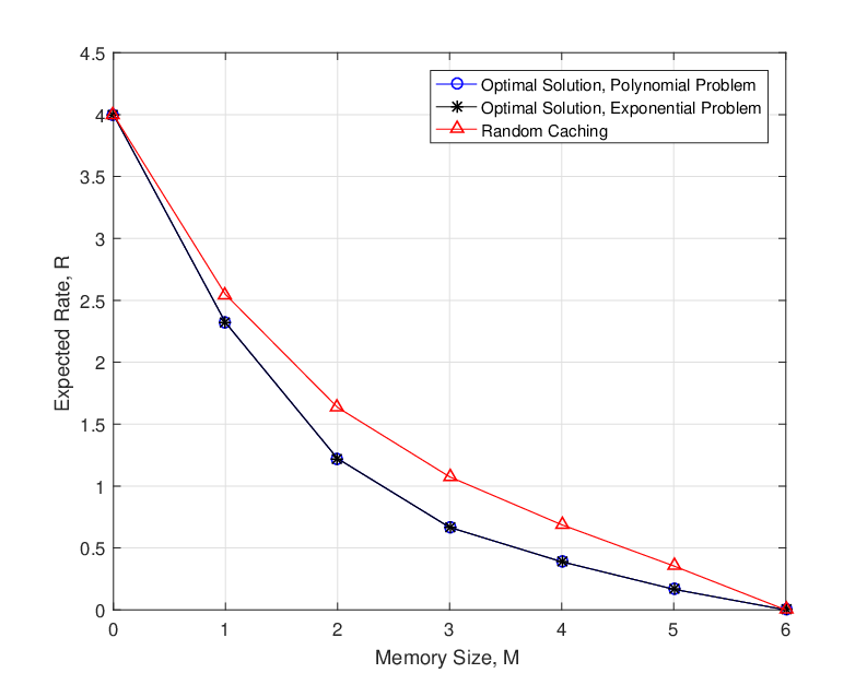
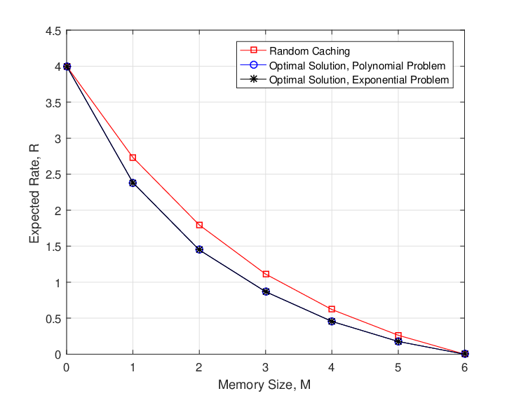
Refer to caption — Fig. 1: A comparison of the performance of the solution obtained from (8)-(9) to the solution obtained by (37)-(38), with reference to a baseline random caching scheme, for the case of non-uniform file popularity only

Both figures show that the performance of the general problem and the two simplified problems is identical for the respective cases considered here. Indeed, when the numerical solutions of (8)-(9) for these two cases are examined explicitly, it is clear that the memory constraint conditions are indeed satisfied, and so the optimal solutions in these cases are attainable by the respective simplified problems.

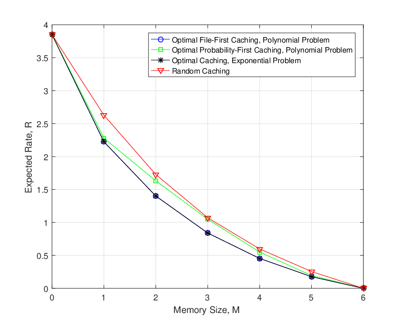
Next, Fig. 3 compares the performance of the original problem (8)-(9) to both the length-first and popularity-first simplified problems for the case of non-uniform file length and popularity. The specific pairings of length and popularities used and their associated labels are listed in Table I.

Although somewhat arbitrary, these file length and popularity combinations are intended to simulate a practical scenario where file popularity and length are relatively uncorrelated. While examining this individual case is not sufficient for determining general patterns, it is enough to gain some important insight about the tension between file length and popularity.

TABLE I: The file labelling and length-popularity pairings used in the non-uniform file popularity and length case.

Length-First (LF) and Popularity-First (PF) Labelling
LF File Index	PF File Index	Length	Popularity
1	5	9/6	0.1176
2	3	8/6	0.1566
3	2	7/6	0.1965
4	6	5/6	0.1062
5	1	4/6	0.2897
6	4	3/6	0.1333

Fig. 3 shows that in this case, the length-first scheme yields much better results than the popularity-first scheme. Indeed, the length-first scheme obtains the same performance as the original problem for all $M$ considered except $M=1$ . The reason for this divergence can be seen from Table II which shows the optimal solution to the original problem (8)-(9) in the $M=1$ case. The value of $|W^{(l)}_{\mathcal{S}}|$ is shown in the $l$ -th column of the row labelled with $\mathcal{S}$ , and the files are ordered using the length-first labelling of Table I. It is clear that file 1, the largest file but fifth-most popular, has been allocated less cache memory than files 2 and 3, which are the third and second most popular files respectively. Thus the memory-inequality constraint (39) is violated and so the length-first simplified problem cannot attain the optimal solution of (8)-(9). Despite this, the optimal value to the simplified problem is only about $10^{-4}$ larger than the optimal value of (8)-(9), and so the difference is not significant. It would thus appear that, while probability cannot be completely ignored in theory, a length-first approach to caching can yield very good results in practice. This insight is later used in Section VI-A, but first the problem of non-uniform cache size must be studied on its own first; this is done next.

TABLE II: Optimal subfile sizes and memory allocation for the general problem (8)-(9) with

K=4,N=6

M=1

, and file lengths and popularities given in Table I (using length-first indexing), with values rounded to three decimal places.

	File Index
Subset	1	2	3	4	5	6
$\emptyset$	0.833	0.583	0.417	0.167	0	0
$\{1\}$	0.167	0.188	0.188	0.167	0.167	0.125
$\{2\}$	0.167	0.188	0.188	0.167	0.167	0.125
$\{3\}$	0.167	0.188	0.188	0.167	0.167	0.125
$\{4\}$	0.167	0.188	0.188	0.167	0.167	0.125
$\{1,2\}$	0	0	0	0	0	0
$\dots$	$\dots$
$\{1,2,3,4\}$	0	0	0	0	0	0
Total memory:	0.167	0.188	0.188	0.167	0.167	0.125

V Coded Caching with Heterogeneous Cache Sizes

We next consider simplifying the optimization formulation for the case with non-uniform cache sizes. For now, file popularity and file length are kept uniform; the case with all parameters being non-uniform is treated in the subsequent section. For the case of non-uniform cache size, a decentralized coded caching scheme is developed in [24] and subsequently improved upon in the $K>N$ case by [25, 26]. As previously discussed, [27] uses an optimization framework similar to the one used in this paper to generate a scheme for the centralized case. For the sake of completion, we note again the work [19] in which the rate region for both non-uniform cache and file size is characterized for $K=2$ users and $N=2$ files, but the optimal scheme is not yet known for the general case.

V-A Optimization Formulation

We first consider a simple case where there are only two cache sizes, “large” and “small”, represented by $M_{L}$ and $M_{S}$ respectively. The variable $K_{L}$ is used to represent the number of users with large caches, and $K_{S}$ is used to represent the number of users with small caches, such that $K_{L}+K_{S}=K$ . Note that file lengths and popularities are fixed as uniform, i.e. $p_{1}=\dots=p_{N}=1/N$ and $F_{1}=\dots=F_{N}=F=1$ respectively.

Since files here are equally popular and of the same size, we have symmetry across files, but now the symmetry across users is broken by the non-uniform cache size. However, certain user symmetry still exists, i.e., symmetry among members of the same cache size group. We therefore define three sets of variables for $j\in[0:K]$ , denoted $v_{j,S},v_{j,L}$ , and $v_{j,M}$ , as follows. For a subset of users $\mathcal{S}$ with a size $|\mathcal{S}|=j$ ,

|W^{(l)}_{S}|=\begin{cases}v_{j,S}&\text{if $\mathcal{S}$ contains only small-cache users,}\\ v_{j,L}&\text{if $\mathcal{S}$ contains only large-cache users,}\\ v_{j,M}&\text{otherwise},\\ \end{cases}

(43)

for all files $l\in[N]$ .

This definition suggests some natural constraints. First, since there are only $K_{S}$ small-cache users, there cannot be a group of $j$ small-cache users if $j>K_{S}$ , so we set

v_{j,S}=0,\forall j>K_{S}.

(44)

Similarly, for large-cache users,

v_{j,L}=0,\forall j>K_{L}.

(45)

A similar constraint is required for the $v_{1,M}$ . Since there cannot be a subset of size one with both large- and small-cache users, we require

v_{1,M}=0;

(46)

Moreover, since the $j=0$ variables correspond to subsets of size 0, it it not particularly meaningful to discuss whether or note this corresponds to a small, large, or mixed subset. To avoid any further complications, we simply set

v_{0,S}=v_{0,L}=v_{0,M}=v_{0}\,,

(47)

To understand the file reconstruction condition, note that, for $j\geq 2$ , there are $\binom{K_{S}}{j}$ groups of small-cache users, $\binom{K_{L}}{j}$ groups of large-cache users, and

\sum_{i=1}^{j-1}\binom{K_{S}}{i}\binom{K_{L}}{j-i}

mixed groups, because each mixed group must have at least one small-cache users and at least one-large cache user. By adding and subtracting the $i=0$ and $i=j$ terms and using Lemma 1, we can rewrite this as

\sum_{i=0}^{j}\binom{K_{S}}{i}\binom{K_{L}}{j-i}-\binom{K_{L}}{j}-\binom{K_{S}}{j}\\ =\binom{K}{j}-\binom{K_{L}}{j}-\binom{K_{S}}{j},

(48)

and so the total portion of the file cached by subsets of size $j\geq 2$ is

\binom{K_{L}}{j}(v_{j,L}-v_{j,M})+\binom{K_{S}}{j}(v_{j,S}-v_{j,M})+\binom{K}{j}v_{j,M}.

(49)

For $j=1$ , there are $K_{L}=\binom{K_{L}}{1}$ large users and $K_{S}=\binom{K_{S}}{1}$ small users. Moreover, since $v_{1,M}=0$ , it is easy to see that (49) also holds for $j=1$ . Finally, consider the $j=0$ case. Here we only need to add $v_{0}$ to capture the portion of the file not cached by any user. However, note that if we set $j=0$ in (49) and apply constraint (47), the first two terms become 0, while the last term reduces to $v_{0,M}=v_{0}$ . Thus (49) applies for all $j$ , and so we can conveniently express the file reconstruction constraint as

\sum_{j=0}^{K}\binom{K_{L}}{j}(v_{j,L}-v_{j,M})+\binom{K_{S}}{j}(v_{j,S}-v_{j,M})\\ +\binom{K}{j}v_{j,M}=1.

(50)

Similar reasoning is used to obtain the cache memory constraints. A small cache user caches every subfile labelled with a subset in which he is contained as a member, and so necessarily caches only subfiles of size $v_{j,S}$ and $v_{j,M}$ . Specifically, a small-cache user is a member of $\binom{K_{S}-1}{j-1}$ small groups of size $j$ , and

\sum_{i=0}^{K-2}\binom{K_{S}-1}{i}\binom{K_{L}}{j-1-i}

(51)

mixed groups. Using Lemma 1 once again, the cache memory constraint for the small user is obtained as

\displaystyle\sum_{j=1}^{K}\binom{K_{S}-1}{j-1}(v_{j,S}-v_{j,M})+\binom{K-1}{j-1}v_{j,M}=M_{S}/N.

(52)

Note that the $j=1$ expression reduces to $\binom{K_{L}-1}{0}(v_{1,S}-0)+0=v_{1,S}$ , as desired. Note also that each file is allocated an equal $M_{S}/N$ of the cache because the files are equally sized and equally popular. Using similar reasoning for large-cache users, we obtain

\displaystyle\sum_{j=1}^{K}\binom{K_{L}-1}{j-1}(v_{j,L}-v_{j,M})+\binom{K-1}{j-1}v_{j,M}=M_{L}/N.

(53)

As always, it is required that all subfiles be of nonnegative size:

\displaystyle v_{j,S}\geq 0,v_{j,L}\geq 0,v_{j,M}\geq 0,\forall j\in\{0,\dots,K\}.

(54)

Finally, the memory inequality constraints for this problem are introduced. In general, we would expect the subfiles that large users have cached to be longer than the ones cached by small users. This is codified in the problem explicitly with

$\displaystyle v_{j,L}\geq$	$\displaystyle\,\,v_{j,M},\,\,j\in[2:K_{L}]$	(55)
$\displaystyle v_{j,M}\geq$	$\displaystyle\,\,v_{j,S},\,\,j\in[2:K_{S}]$	(56)
$\displaystyle v_{j,L}\geq$	$\displaystyle\,\,v_{j,S},\,\,j\in[1:K_{L}].$	(57)

Again note that there is some redundancy in these constraints, but they are nonetheless included for clarity of exposition. Note also that the first two inequalities hold from $j=2$ to $j=K_{L}$ and $j=K_{S}$ respectively; the $j=1$ is already constrained by (46), while the $j=0$ is constrained by (47), and the $j>K_{L}$ and $j>K_{S}$ cases are governed by (45) and (44) respectively.

As Proposition 3 shows, the memory inequality constraints allow us to greatly simplify the original objective function (8).

Proposition 3.

Assuming uniform file length and popularity but two different user cache sizes, and with variables as defined in (43) and satisfying (44)-(47) and (54)-(57), the objective function (8) simplifies exactly as

\mathbb{E}\left[\sum_{\mathcal{S}\in\mathcal{P}(\mathcal{U})\setminus\emptyset}\max_{k\in\mathcal{S}}\{|W_{S\setminus\{k\}}^{(d_{k})}|\}\right]\\ =\sum_{j=0}^{K-1}\binom{K_{s}}{j+1}(v_{j,S}-v_{j,M})+\binom{K}{j+1}v_{j,M}+\\ \quad\left(\binom{K_{L}}{j+1}+\binom{K_{S}}{1}\binom{K_{L}}{j}\right)(v_{j,L}-v_{j,M})

(58)

The proof of Proposition 3 is in Appendix -C. The simplified optimization problem can then be written as

minimize	$\displaystyle\sum_{j=0}^{K-1}\binom{K_{s}}{j+1}(v_{j,S}-v_{j,M})+\binom{K}{j+1}v_{j,M}+$
	$\displaystyle\quad\left(\binom{K_{L}}{j+1}+\binom{K_{S}}{1}\binom{K_{L}}{j}\right)(v_{j,L}-v_{j,M})$	(59)
subject to	$\displaystyle\text{ \eqref{firstofmany}-\eqref{allequal}, \eqref{6thfirstconstraint}, \eqref{6thsecondconstraintp1}-\eqref{6thfifthconstraintp3}}.$	(60)

This is a linear program that has a number of variables, constraints, and objective function summands that scale linearly in $K$ .

Finally, we remark that only two cache sizes were considered in this paper. While a practical system would likely have more than two cache sizes, it is reasonable to expect that only a small number of cache sizes will be used, e.g. cell phones with 8,16, 32 or 64 GB of cache memory. The reasoning used here for two cache sizes could then be extended to accommodate these additional cache sizes as needed.

V-B Numerical Results

Consider a case where there are $N=6$ files, uniform in popularity and length, and $K=4$ users. Define a ”memory factor” $M\in[0:N]$ ; there are $K_{S}$ small users with a cache size of $M_{S}=0.8M$ , and $K_{L}$ large users with a cache size of $M_{L}=1.2M$ . Fig. 4 compares the corresponding solution of the general problem (8)-(9) to the solution of the simplified problem (59)-(60) when there are $K_{S}=2$ small users. The random caching scheme of [24] is included, but the centralized scheme of [27] (which has exponential complexity) is not. The purpose here is not to determine the best caching scheme for the heterogeneous cache case, but to, first, demonstrate the implicit performance-tractability tradeoff of using the simplified problem (59)-(60) over the general problem, and second, to demonstrate that it is worth the effort of developing and using these problems to design cache content (rather than caching randomly) when the engineering context allows for it. Nevertheless, we expect the performance of the problem in [27] to be very similar, if not identical, to the exponential problem developed here, even though the two optimization frameworks are not identical themselves. Table III also shows the optimal cache content obtained from the general problem in the $K_{S}=2$ , $M=4$ case.

TABLE III: Optimal subfile sizes and memory allocation for the general problem (8)-(9) with

K=4,N=6

K_{S}=2

M_{S}=3.2

and

M_{L}=4.8

, with values rounded to three decimal places.

	File Index
Subset	1	2	3	4	5	6
$\emptyset$	0	0	0	0	0	0
$\dots$	$\dots$
$\{4\}$	0	0	0	0	0	0
$\{1,2\}$	0.056	0.056	0.056	0.056	0.056	0.056
$\{1,3\}$	0.056	0.056	0.056	0.056	0.056	0.056
$\{1,4\}$	0.056	0.056	0.056	0.056	0.056	0.056
$\{2,3\}$	0.056	0.056	0.056	0.056	0.056	0.056
$\{2,4\}$	0.056	0.056	0.056	0.056	0.056	0.056
$\{3,4\}$	0.056	0.056	0.056	0.056	0.056	0.056
$\{1,2,3\}$	0.033	0.033	0.033	0.033	0.033	0.033
$\{1,2,4\}$	0.033	0.033	0.033	0.033	0.033	0.033
$\{1,3,4\}$	0.300	0.300	0.300	0.300	0.300	0.300
$\{2,3,4\}$	0.300	0.300	0.300	0.300	0.300	0.300
$\{1,2,3,4\}$	0	0	0	0	0	0
Mem. (L):	0.800	0.800	0.800	0.800	0.800	0.800
Mem. (S):	0.533	0.533	0.533	0.533	0.533	0.533

Fig. 4 shows that in the $K_{S}=2$ case, while the simplified problem tracks the optimal scheme for small cache size ( $M\leq 3$ ), it performs worse than even the random caching scheme for large $M$ values. Table III reveals why this is the case. Here, users 1 and 2 are the small users, and users 3 and 4 are the large users. The variable definitions in (43) specify one variable for all mixed subsets of the same size, but consider the subfile sizes for the size-three subsets: the subsets with 2 small users have smaller subfiles than the subsets with 2 large users. Thus using only one $v_{l,j}^{M}$ variable for these four subsets results in a loss in performance. In principle, one could introduce more variables to accommodate this, albeit at a cost of a more complicated objective function.

VI Coded Caching with Heterogeneous Files and Cache Sizes

The natural final step in this program is to develop a tractable optimization problem that accommodates non-uniformity in cache size, file size, and popularity at the same time. To the best of our knowledge, there has yet to be a caching scheme proposed that handles heterogeneity in all three of these domains.

VI-A Optimization Formulation

We begin by defining a new set of variables that, in a sense, combines the functionality of the variables defined in (30) and (43). Let

|W^{(l)}_{S}|=\begin{cases}v^{S}_{l,j}&\text{if $\mathcal{S}$ contains only small-cache users,}\\ v^{L}_{l,j}&\text{if $\mathcal{S}$ contains only large-cache users,}\\ v^{M}_{l,j}&\text{otherwise},\\ \end{cases}

(61)

for a subset of users $\mathcal{S}$ such that $|\mathcal{S}|=j$ and all files $l\in[N]$ . The symmetry across users is broken by the heterogeneity of the user cache size, and the symmetry across files is broken by a the heterogeneity of files in both length and popularity. Nevertheless, we can still exploit the symmetry across subsets of users of the same size ( $j$ ) and type (i.e. small, large, mixed) for a particular file ( $l$ ) to reduce the complexity of the original problem (8)-(9) while still accounting for the aforementioned heterogeneity.

Many of the constraints used in the non-uniform cache size case can be converted to their equivalents for this new case. If $j>K_{S}$ , there cannot be a subset of $j$ small cache users, so

v_{l,j}^{S}=0,\forall j>K_{S},\forall l\in[N],

(62)

and similarly

v_{l,j}^{L}=0,\forall j>K_{L},\forall l\in[N].

(63)

Since there cannot be a subset of size 1 containing both large and small users, the $l=1$ variable is constrained as

v_{l,1}^{M}=0,\forall l\in[N],

(64)

and for convenience, we set

v_{l,0}^{S}=v_{l,0}^{L}=v_{l,0}^{M}=v_{l,0},\forall l\in[N].

(65)

The cache size-based memory inequalities should still hold, giving, for a fixed file $l$ ,

$\displaystyle v_{l,j}^{L}\geq$	$\displaystyle\,\,v_{l,j}^{M},\,\,j\in[2:K_{L}],\forall l\in[N],$	(66)
$\displaystyle v_{l,j}^{M}\geq$	$\displaystyle\,\,v_{l,j}^{S},\,\,j\in[2:K_{S}],\forall l\in[N],$	(67)
$\displaystyle v_{l,j}^{L}\geq$	$\displaystyle\,\,v_{l,j}^{S},\,\,j\in[1:K_{L}],\forall l\in[N].$	(68)

We also import conditions from the non-uniform file size and popularity problem. As seen earlier, it is better to prioritize file length rather than popularity, and so we label the files in decreasing order of file length. This gives

$\displaystyle v_{l_{1},j}^{L}\geq$	$\displaystyle\,\,v_{l_{2},j}^{L},\,j\in[0:K-1],\forall l_{1},l_{2}\text{ s.t. }l_{1}<l_{2}$	(69)
$\displaystyle v_{l_{1},j}^{M}\geq$	$\displaystyle\,\,v_{l_{2},j}^{M},\,j\in[0:K-1],\forall l_{1},l_{2}\text{ s.t. }l_{1}<l_{2}$	(70)
$\displaystyle v_{l_{1},j}^{S}\geq$	$\displaystyle\,\,v_{l_{2},j}^{S},\,j\in[0:K-1],\forall l_{1},l_{2}\text{ s.t. }l_{1}<l_{2}.$	(71)

The remaining conditions are formed using identical reasoning to the non-uniform cache case, but occur on a file-by-file basis as needed. The file reconstruction constraint remains the same, with the minor change that the file must add up not to the common file length 1, but to $F_{l},$ the actual length of the file as expressed below:

F_{l}=\sum_{j=0}^{K}\binom{K_{L}}{j}(v_{l,j}^{L}-v_{l,j}^{M})+\binom{K_{S}}{j}(v_{l,j}^{S}-v_{l,j}^{M})\\ +\binom{K}{j}v_{l,j}^{M},\qquad\forall l\in[N]

(72)

The cache memory constraints are modified similarly, except instead of giving an equal amount $M_{S}/N$ to each file, an amount $\mu_{l}^{S}$ is allocated to file $l$ , yielding

\mu_{l}^{S}=\sum_{j=1}^{K}\binom{K_{S}-1}{j-1}(v_{l,j}^{S}-v_{l,j}^{M})\\ +\binom{K-1}{j-1}v_{l,j}^{M},\qquad\forall l\in[N],

(73)

where it must be the case that

\sum_{l=1}^{N}\mu_{l}^{S}=M_{S}.

(74)

A similar pair of equations holds for large users:

\mu_{l}^{L}=\sum_{j=1}^{K}\binom{K_{L}-1}{j-1}(v_{l,j}^{L}-v_{l,j}^{M})\\ +\binom{K-1}{j-1}v_{l,j}^{M},\qquad\forall l\in[N],

(75)

and

\sum_{l=1}^{N}\mu_{l}^{L}=M_{L}.

(76)

The subfiles are also required to be positive in size, as always:

\displaystyle v_{l,j}^{L}\geq 0,\,v_{l,j}^{S}\geq 0,\,v_{l,j}^{M}\geq 0,\,\forall j\in[0:K],\,l\in[N]

(77)

Finally, another set of memory inequality constraints are required to break ties between small-index, small-cache subfiles and large-index, large-cache subfiles. Leaving the justification and discussion of this choice to later sections, we develop a caching scheme under the constraints

$\displaystyle v_{l_{1},j}^{L}\geq$	$\displaystyle\,\,v_{l_{2},j}^{M},\,\,j\in[2:K_{L}],\,\,\forall l_{1},l_{2}\in[N]$	(78)
$\displaystyle v_{l_{1},j}^{M}\geq$	$\displaystyle\,\,v_{l_{2},j}^{S},\,\,j\in[2:K_{S}],\,\,\forall l_{1},l_{2},\in[N]$	(79)
$\displaystyle v_{l_{1},j}^{L}\geq$	$\displaystyle\,\,v_{l_{2},j}^{S},\,\,j\in[1:K_{L}],\,\,\forall l_{1},l_{2}\in[N].$	(80)

In words, this means that subfiles for any file stored on a larger cache type should be larger than the subfiles of any file stored on a smaller cache type, independent of which files are involved. The following proposition gives the objective function of the simplified optimization problem.

Proposition 4.

Define the following functions of the integer parameters $n,m,j$ and $i$ :

$\displaystyle\nu_{1}(n,m,j,i)$	$\displaystyle=$	$\displaystyle\left(\frac{K_{S}-m}{K-n+1}\right)$
		$\displaystyle\binom{K_{S}-m-1}{i}\binom{K_{L}-n+1+m}{j-i},$
$\displaystyle\nu_{2}(n,m,j,i)$	$\displaystyle=$	$\displaystyle\left(\frac{K_{L}-n+1+m}{K-n+1}\right)$
		$\displaystyle\binom{K_{S}-m}{i}\binom{K_{L}-n+m}{j-i},$

and

	$\displaystyle\nu(n,j)$	$\displaystyle=$	$\displaystyle\sum_{m=0}^{n-1}\frac{\binom{K_{S}}{m}\binom{K_{L}}{n-1-m}}{\binom{K}{n-1}}$
			$\displaystyle\left(\sum_{i=1}^{j-2}\nu_{1}(n,m,j,i)+\sum_{i=2}^{j-1}\nu_{2}(n,m,j,i)\right)$

Then for the variables defined in (61) satisfying (62)-(80), the objective function (8) simplifies exactly as

		$\displaystyle\mathbb{E}\left[\sum_{\mathcal{S}\in\mathcal{P}(\mathcal{U})\setminus\emptyset}\max_{k\in\mathcal{S}}\{\|W_{S\setminus\{k\}}^{(d_{k})}\|\}\right]$
		$\displaystyle\,\,=\sum_{i=0}^{K-1}\sum_{l=1}^{N}\text{Pr}[Y_{i}=l]v_{l,0}^{M}$
		$\displaystyle\quad+\sum_{j=1}^{K_{L}-1}\sum_{i=0}^{K_{L}-1}\sum_{l=1}^{N}\binom{K_{L}-1-i}{j}\text{Pr}[Y_{i}^{L}=l]v_{l,j}^{L}$
		$\displaystyle\quad+\sum_{j=1}^{K_{S}-1}\sum_{i=0}^{K_{S}-1}\sum_{l=1}^{N}\binom{K_{S}-1-i}{j}\text{Pr}[Y_{i}^{S}=l]v_{l,j}^{S}$
		$\displaystyle\quad+\sum_{j=1}^{K_{L}}\sum_{i=0}^{K_{S}-1}\sum_{l=1}^{N}\binom{K_{L}}{j}\text{Pr}[Y_{i}^{S}=l]v_{l,j}^{L}$
		$\displaystyle\quad+\sum_{j=2}^{K_{S}-1}\sum_{i=0}^{K_{S}-1}\sum_{l=1}^{N}\binom{K_{S}-1-i}{j}\binom{K_{L}}{1}\text{Pr}[Y_{i}^{S}=l]v_{l,j}^{M}$
		$\displaystyle\quad+\sum_{j=\max\{K_{S},K_{L}\}+1}^{K-1}\sum_{i=0}^{K-1}\sum_{l=1}^{N}\binom{K-1-i}{j}\text{Pr}[Y_{i}=l]v_{l,j}^{M}$
		$\displaystyle\quad+\sum_{j=3}^{\max\{K_{S},K_{L}\}}\sum_{n=1}^{K}\sum_{l=1}^{N}\text{Pr}[Y_{n-1}=l]\nu(n,j)v_{l,j}^{M}$		(81)

Proposition 4 is proved in Appendix -D. Although visually complicated, (81) simplifies the original objective function (8) by using only $3(K+1)N$ variables and having a number of terms that scales with $K^{2}N$ rather than $(2N)^{K}$ . The number of constraints described by (62)-(80) scales with $KN^{2}$ , and so the following optimization problem is a tractable method of obtaining a caching scheme that accommodates heterogeneity in cache size, file size, and file popularity:

	minimize	(81)		(82)
	subject to	$\displaystyle\eqref{2ndfirstofmany}-\eqref{7thfinconstraintp3}$		(83)

VI-B Numerical Results

To demonstrate that this simplified optimization problem performs well when compared to the general problem (8)-(9), we again consider $K=4$ users ( $K_{S}=2$ of which are small-cache users) and $N=6$ files, with all of the non-uniformities used thus far: file labels and popularity/size pairs as given in Table I, and cache sizes of $M_{S}=0.8M$ and $M_{L}=1.2M$ for $M\in[0:N]$ . Fig. 5 compares the simplified and general problems with a naive random caching baseline.

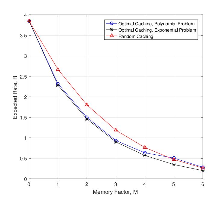
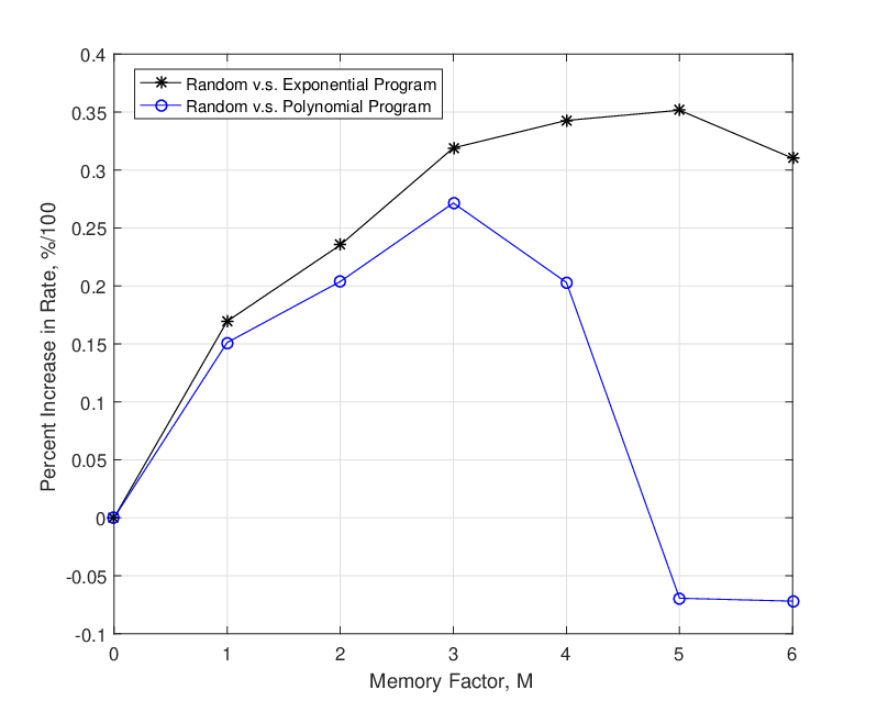
We see that the simplified problem yields a scheme that closes mirrors, although does not match exactly, the performance of the scheme obtained from the general problem for small and intermediate $M$ values. Table IV shows the optimal solution to the general problem for the $M=2$ case; we see several violations of the memory inequality constraints that explain why the simplified problem could not achieve as good a performance as the general problem: the “true” optimal solution lies outside of its feasible space. Nevertheless, the simplified problem still achieves good performance compared to the general problem in this regime. For large $M$ , we see that the expected rate of the simplified scheme does not drop as quickly as the general problem solution, and is even eclipsed by the random caching scheme. This occurs for the same reason we saw in Section V in the $K_{S}=2$ case (Fig. 4). To compare the relative performance of the three schemes in general, Fig. 6 shows the percent increase in expected rate if the random caching scheme is used over the general and simplified schemes respectively. The significant increase in rate when using random caching make it clear that designing the cache content can be worthwhile when the engineering context allows for it.

TABLE IV: Optimal subfile sizes and memory allocation for the general problem (8)-(9) with

K=4,N=6

K_{S}=2

M_{S}=1.6

M_{L}=2.4

and file popularity/ size pairs given by Table I, with values rounded to three decimal places.

	File Index
Subset	1	2	3	4	5	6
$\emptyset$	0	0	0	0	0	0
$\{1\}$	0.178	0.178	0.178	0.178	0.165	0.085
$\{2\}$	0.178	0.178	0.178	0.178	0.165	0.085
$\{3\}$	0.178	0.178	0.178	0.178	0.165	0.085
$\{4\}$	0.178	0.178	0.178	0.178	0.165	0.085
$\{1,2\}$	0	0.077	0.008	0	0	0
$\{1,3\}$	0.090	0.090	0.090	0.008	0	0
$\{1,4\}$	0.090	0.090	0.090	0.008	0	0
$\{2,3\}$	0.090	0.090	0.090	0.008	0	0
$\{2,4\}$	0.090	0.090	0.090	0.008	0	0
$\{3,4\}$	0.431	0.188	0.090	0.090	0.008	0
$\{1,2,3\}$	0	0	0	0	0	0
$\dots$	$\dots$
$\{1,2,3,4\}$	0	0	0	0	0	0
Mem. (L):	0.788	0.554	0.446	0.284	0.173	0.165
Mem. (S):	0.357	0.434	0.365	0.194	0.165	0.085

VI-C Further Extensions

We first echo the earlier comments about heterogeneous cache sizes: we consider only two different cache sizes here, but it is possible to use the same reasoning to develop a tractable optimization problem for a practical system having more (but not many more) cache sizes.

The primary focus in this section, however, is on the memory inequality constraints (78)-(80) used in developing the simplified problem (82)-(83) of this section. Recall that these constraints require, among other things, that (roughly speaking) for a fixed index $j$ , the $v^{L}_{l,j}$ variables for all files $l$ be larger than the $v^{S}_{l,j}$ variables for all files. Thus the large-user subfile for the smallest file is larger than the small-user subfile for the largest file. This restriction was required to allow us to write the simplified problem, and numerical results show that the simplified problem still performed well compared to the general problem for the considered parameters. While a full investigation of the performance of the simplified problem across all parameter values would be labourious, it is still possible to estimate the behaviour for certain parameter regimes. We should expect (78)-(80) to result in a good simplification when the disparity between the large and small cache sizes is big, and when there are small numbers of files, because the large cache users will likely store much larger subfiles than the small cache users, irrespective of the length of the file. Conversely, we should expect the performance of (82)-(83) to be relatively poor when the cache sizes are comparable and there are large numbers of files. In this case, it may make more sense to use something like the “opposite” memory inequality constraint: a small-user subfile variable $v^{S}_{l_{1},j}$ should be larger than any larger-user subfile variable $v^{L}_{l_{2},j}$ if file $l_{1}$ is larger than file $l_{2}$ . While the simplified optimization problem that would result from this constraint is not explored in this paper, it should be possible to construct such a problem using the same kind of reasoning used here.

Indeed, there may also be other memory inequality constraints that prove to yield useful simplified optimization problems for other parameter sets. The appeal of the tractability of these models is that a server, knowing the relevant parameters for its system, could easily compute the performance of these schemes and choose the best among them; any discussion of the specifics of such schemes, however, is left to future work.

VII Summary and Conclusions

The two primary goals of this paper are to advance a certain optimization theoretic approach to coded caching problems, and to use that framework to derive both specific caching schemes and general insight for system models containing multiple heterogeneities that have yet to be considered in the literature. An exponentially-scaling optimization problem corresponding to a caching scheme capable of handling non-uniform file size, popularity, and cache size is developed. It is shown that the original scheme of Maddah-Ali and Niesen in [2, 3] is the optimal solution of that problem for the special case of uniform file length, popularity, and cache size.

Tractable problems are then developed to handle various combinations of heterogeneous system parameters. The consideration of these special cases also permitted the observation of the effects that these non-uniformities have on the optimal cache content. When considering non-uniform file popularity and size jointly, it is shown that while popularity may in general have some influence on the optimal cache allocation, file size can be a much stronger influence; indeed, very good performance is obtained in the case considered by ignoring file popularity altogether. Finally, with the insights obtained from the previously-explored special cases, we developed a tractable optimization problem corresponding to a caching scheme capable of accommodating all three of the aforementioned heterogeneities, and showed numerically that it performs well compared to the original exponentially-scaling problem.

-A Proof of Lemma 2

We begin with the proof of the expression of $\text{Pr}[Y_{0}=i]$ , for which we use induction on $i$ for $i=1,\dots,N$ . We begin first with the $i=1$ case. Let $\mathbf{Z}\in[N]^{K}$ denote the sequence of outcomes from the $N$ trials, e.g. if for $K$ = 3 and $N$ = 4, trial 1 obtains outcome 2, trial 2 obtains outcome 4, and trial 3 obtains outcome 1, we have $\mathbf{Z}=[2,4,1]^{T}$ . Let $X_{n}$ denote the random variable representing the number of times the outcome $n$ occurs in the $K$ trials (i.e. the number of times it appears in $\mathbf{Z}$ ), and stack the $X_{n}$ variables in a vector $\mathbf{X}\in[K]^{N}$ ; the example above would yield $\mathbf{X}=[1,1,0,1]^{T}$ . Then the smallest element of $\mathbf{Z}$ is 1 (i.e. $Y_{0}=1$ ) if and only if $X_{1}>=1$ ; in other words, since 1 is the smallest possible outcome, if it occurs anywhere in $\mathbf{Z}$ then it is the smallest element. Thus we have

	$\displaystyle\text{Pr}[Y_{0}=1]$	$\displaystyle=$	$\displaystyle\text{Pr}[X_{1}\geq 1]=1-\text{Pr}[X_{1}=0]$
		$\displaystyle=$	$\displaystyle 1-(1-p_{1})^{K}=\left(\sum_{l=1}^{N}p_{l}\right)^{K}-\left(\sum_{l=2}^{N}p_{l}\right)^{K},$

which is indeed the formula (26) with $i=1$ , as desired.

For an arbitrary $i$ such that $2\leq i\leq N-1$ , we note that if the smallest element of $\mathbf{Z}$ is $i$ , (i.e. $Y_{0}=i$ ), then there cannot be any values smaller than $i$ , and there must be at least one $i$ in $\mathbf{Z}$ ; in other words:

$\displaystyle\text{Pr}[Y_{0}=i]$	$\displaystyle=\text{Pr}[X_{i}\geq 1,X_{i-1}=0,\dots X_{1}=0]$
	$\displaystyle=\text{Pr}[X_{1}=0]\text{Pr}[X_{2}=0\|X_{1}=0]\cdots$
	$\displaystyle\quad\text{Pr}[X_{i-1}=0\|X_{i-2}=\dots=X_{1}=0]$
	$\displaystyle\quad\text{Pr}[X_{i}\geq 1\|X_{i-1}=\dots=X_{1}=0]$
	$\displaystyle=\text{Pr}[X_{1}=0]\text{Pr}[X_{2}=0\|X_{1}=0]\cdots$
	$\displaystyle\quad\text{Pr}[X_{i-1}=0\|X_{i-2}=\dots=X_{1}=0]$
	$\displaystyle\quad\left(1-\text{Pr}[X_{i}=0\|X_{i-1}=\dots=X_{1}=0]\right).$	(84)

Now, comparing the expression (84) for $Y_{0}=i$ to the same expression with $Y_{0}=i-1$ , it is easy to show that

$\displaystyle\text{Pr}[Y_{0}=i]$	$\displaystyle=\text{Pr}[Y_{0}=i-1]$
	$\displaystyle\quad\left(\frac{\text{Pr}[X_{i-1}=0\|X_{i-2}=\dots=X_{1}=0]}{1-\text{Pr}[X_{i-1}=0\|X_{i-2}=\dots=X_{1}=0]}\right)$
	$\displaystyle\quad\left(1-\text{Pr}[X_{i}=0\|X_{i-1}=\dots=X_{1}=0]\right).$	(85)

It is possible to compute these conditional probabilities directly:

\displaystyle\text{Pr}[X_{j}=0|X_{j-1}=\dots=X_{1}=0]=\left(1-p_{j}^{(j)}\right)^{K},

(86)

where

p_{j}^{(j)}=\frac{p_{j}}{\sum_{l=j}^{N}p_{l}}

is the probability of outcome $j$ occurring in a trial conditioned on the knowledge that outcomes 1 through $j-1$ have not occurred in that trial. From the definition of $p_{j}^{(j)}$ , we can rewrite (86) as

\text{Pr}[X_{j}=0|X_{j-1}=\dots=X_{1}=0]=\left(\frac{\sum_{l=j+1}^{N}p_{l}}{\sum_{l=j}^{N}p_{l}}\right)^{K}.

Evaluating this expression for $j=i$ and $j=i-1$ , we can obtain from (85), after some mild algebraic manipulation,

	$\displaystyle\text{Pr}[Y_{0}=i]=$	$\displaystyle\,\,\text{Pr}[Y_{0}=i-1]\left(\frac{\sum_{l=i}^{N}p_{l}}{\sum_{l=i-1}^{N}p_{l}}\right)^{K}$
		$\displaystyle\frac{\left(\sum_{l=i-1}^{N}p_{l}\right)^{K}}{\left(\sum_{l=i-1}^{N}p_{l}\right)^{K}-\left(\sum_{l=i}^{N}p_{l}\right)^{K}}$
		$\displaystyle\frac{\left(\sum_{l=i}^{N}p_{l}\right)^{K}-\left(\sum_{l=i+1}^{N}p_{l}\right)^{K}}{\left(\sum_{l=i}^{N}p_{l}\right)^{K}}$
	$\displaystyle=$	$\displaystyle\,\,\text{Pr}[Y_{0}=i-1]\frac{\left(\sum_{l=i}^{N}p_{l}\right)^{K}-\left(\sum_{l=i+1}^{N}p_{l}\right)^{K}}{\left(\sum_{l=i-1}^{N}p_{l}\right)^{K}-\left(\sum_{l=i}^{N}p_{l}\right)^{K}}.$

Now by the inductive hypothesis, $\text{Pr}[Y_{0}=i-1]$ is precisely equal to the denominator of (), and so we obtain

\text{Pr}[Y_{0}=i]=\left(\sum_{l=i}^{N}p_{l}\right)^{K}-\left(\sum_{l=i+1}^{N}p_{l}\right)^{K},

(88)

as desired.

Although the $\text{Pr}[Y_{0}=N]$ formula was covered in the preceding paragraph, we discuss it in further detail here because (26) above may not appear sensible in the $i=N$ case. Note that if $N$ is the smallest value in the multinomial vector $\mathbf{Z}$ , then it must be the case that every element of $\mathbf{Z}$ is equal to $N$ , otherwise some element not equal to $N$ would be the smallest value. Thus we have

$\displaystyle\text{Pr}[Y_{0}=N]$	$\displaystyle=$	$\displaystyle\text{Pr}[X_{N}=K,X_{N-1}=0,\dots,X_{1}=0]$
	$\displaystyle=$	$\displaystyle p_{N}^{K}$
	$\displaystyle=$	$\displaystyle\left(\sum_{l=N}^{N}p_{l}\right)^{K}-\left(\sum_{l=N+1}^{N}p_{l}\right)^{K},$

which is the formula (26) with $i=N$ , noting that we use the definition that $\sum_{l=a}^{b}n_{l}=0$ when $a>b$ .

Next, we proceed to the $m=1$ case. Here we will directly compute $\text{Pr}[Y_{1}=i]$ by first deriving $\text{Pr}[Y_{1}=i,Y_{0}=j]$ , and then obtaining the desired quantity from the sum

\text{Pr}[Y_{1}=i]=\sum_{j=1}^{N}\text{Pr}[Y_{1}=i,Y_{0}=j]

(89)

Clearly the second smallest element of $\mathbf{Z}$ is no smaller than the smallest element of $\mathbf{Z}$ , so there are two cases to consider: $i>j$ , and $i=j$ . If $i>j$ , we write

		$\displaystyle\text{Pr}[Y_{1}=i,Y_{0}=j]$
		$\displaystyle\,\,=\text{Pr}[X_{i}\geq 1,X_{i-1}=0,\dots,X_{j}=1,$
		$\displaystyle\quad\qquad X_{j-1}=\dots=X_{1}=0]$
		$\displaystyle\,\,=\text{Pr}[X_{i-1}=0,\dots,X_{j}=1,X_{j-1}=\dots=X_{1}=0]$
		$\displaystyle\quad-\text{Pr}[X_{i}=0,X_{i-1}=0,\dots,X_{j}=1,$
		$\displaystyle\quad\qquad X_{j-1}=\dots=X_{1}=0]$		(90)

To compute the difference (90), note that we can form a ( $K$ , 4) sequential vector of outcomes $\tilde{\mathbf{Z}}(m,n)$ , indexed by two integers $m$ and $n$ , from the original ( $K$ , $N$ ) sequential vector of outcomes $\mathbf{Z}$ in the following way: for a single trial, the first outcome of $\tilde{\mathbf{Z}}(m,n)$ occurs if any of the first $n-1$ outcomes of $\mathbf{Z}$ occur, and so it has the probability $\tilde{p}_{1}=\sum_{l=1}^{n-1}p_{j}$ ; the second outcome of $\tilde{\mathbf{Z}}(m,n)$ occurs if the $n$ -th outcome of $\mathbf{Z}$ occurs, and so it has a probability of $\tilde{p}_{2}=p_{n}$ ; the third outcome of $\tilde{\mathbf{Z}}(m,n)$ occurs if any outcomes of $\mathbf{Z}$ from $n+1$ to $m$ occurs, and so it has a probability of $\tilde{p}_{3}=\sum_{l=n+1}^{m}p_{l}$ ; and the fourth outcome of $\tilde{\mathbf{Z}}(m,n)$ occurs if any of the last $N-m$ outcomes of $\mathbf{Z}$ occur, and so it has a probability $\tilde{p}_{4}=\sum_{l=m+1}^{N}p_{l}$ . If we define $\tilde{X}_{j}$ as the number of times outcome $j$ occurred in $\tilde{\mathbf{Z}}(m,n)$ , then we consequently have $\tilde{X}_{1}=\sum_{l=1}^{n-1}X_{l}$ , $\tilde{X}_{2}=X_{n}$ , $\tilde{X}_{3}=\sum_{l=n+1}^{m}X_{l}$ , and $\tilde{X}_{4}=\sum_{l=m+1}^{N}X_{l}$ . We can then rewrite¹¹ 1 Note that the $\tilde{X}$ variables lose the $(m,n)$ indices of the original variable $\tilde{\mathbf{X}}(m,n)$ . This is done for notational convenience, but will result in an abuse of the notation when multiple $\tilde{\mathbf{X}}(m,n)$ are involved. We will therefore be careful to indicate which $\tilde{X}$ variables belong to which $\tilde{\mathbf{X}}(m,n)$ vectors. (90) using vectors $\tilde{\mathbf{X}}(i,j)$ and $\tilde{\mathbf{X}}(i-1,j)$ as

\text{Pr}[Y_{1}=i,Y_{0}=j]\\ =\text{Pr}[\tilde{X}_{4}=K-1,\tilde{X}_{3}=0,\tilde{X}_{2}=1,\tilde{X}_{1}=0]\\ -\text{Pr}[\tilde{X}_{4}=K-1,\tilde{X}_{3}=0,\tilde{X}_{2}=1,\tilde{X}_{1}=0]

(91)

where the first term is computed with respect to $\tilde{\mathbf{X}}(i-1,j)$ , and the second with respect to $\tilde{\mathbf{X}}(i,j)$ . Using the probabilities defined earlier, this gives

		$\displaystyle\text{Pr}[Y_{1}=i,Y_{0}=j]$
		$\displaystyle\,\,=K\tilde{p}_{2}(\tilde{p}_{4})^{K-1}-K\tilde{p}_{2}(\tilde{p}_{4})^{K-1}$		(92)
		$\displaystyle\,\,=Kp_{j}\left(\left(\sum_{l=i}^{N}p_{l}\right)^{K-1}-\left(\sum_{l=i+1}^{N}p_{l}\right)^{K-1}\right)$		(93)

where, again, the terms in (92) are computed with respect to $\tilde{\mathbf{X}}(i-1,j)$ , and $\tilde{\mathbf{X}}(i,j)$ respectively.

Similar reasoning yields the value of the joint probability when $i=j$ :

		$\displaystyle\text{Pr}[Y_{1}=i,Y_{2}=i]$
		$\displaystyle\,\,=\text{Pr}[X_{i}\geq 2,X_{i-1}=\dots=X_{1}=0]$
		$\displaystyle\,\,=\text{Pr}[X_{i-1}=\dots=X_{1}=0]-\text{Pr}[X_{i}=0=\dots=X_{1}=0]$
		$\displaystyle\quad-\text{Pr}[X_{i}=1,X_{i-1}=\dots=X_{1}=0]$
		$\displaystyle\,\,=\text{Pr}[\tilde{X}_{4}=K,\tilde{X}_{3}=\tilde{X}_{2}=\tilde{X}_{1}=0]$
		$\displaystyle\quad-\text{Pr}[\tilde{X}_{4}=K,\tilde{X}_{3}=\tilde{X}_{2}=\tilde{X}_{1}=0]$
		$\displaystyle\quad-\text{Pr}[\tilde{X}_{4}=K-1,\tilde{X}_{3}=1,\tilde{X}_{2}=\tilde{X}_{1}=0].$		(94)

Here, the first term in (94) is computed with respect to $\tilde{\mathbf{X}}(i-1,i-2)$ , the second with respect to $\tilde{\mathbf{X}}(i,i-1)$ , and the third with respect to $\tilde{\mathbf{X}}(i,i-1)$ , although this choice of $\tilde{\mathbf{X}}$ variables is not unique. This gives

		$\displaystyle\text{Pr}[Y_{1}=i,Y_{2}=i]$
		$\displaystyle\,\,=(\tilde{p}_{4})^{K}-(\tilde{p}_{4})^{K}-K\tilde{p}_{2}(\tilde{p}_{4})^{K-1}$
		$\displaystyle\,\,=\left(\sum_{l=i}^{N}p_{l}\right)^{K}-\left(\sum_{l=i+1}^{N}p_{l}\right)^{K}-Kp_{i}\left(\sum_{l=i+1}^{N}p_{l}\right)^{K-1}.$		(95)

We can now evaluate (89) as

		$\displaystyle\text{Pr}[Y_{1}=i]$
		$\displaystyle\,\,=\sum_{j=1}^{N}\text{Pr}[Y_{1}=i,Y_{0}=j]$
		$\displaystyle\,\,=\sum_{j=1}^{i-1}\text{Pr}[Y_{1}=i,Y_{0}=j]+\text{Pr}[Y_{1}=i,Y_{0}=i]+0$
		$\displaystyle\,\,=\sum_{j=1}^{i-1}\left(Kp_{j}\left(\left(\sum_{l=i}^{N}p_{l}\right)^{K-1}-\left(\sum_{l=i+1}^{N}p_{l}\right)^{K-1}\right)\right)$
		$\displaystyle\quad+\left(\sum_{l=i}^{N}p_{l}\right)^{K}-\left(\sum_{l=i+1}^{N}p_{l}\right)^{K}-Kp_{i}\left(\sum_{l=i+1}^{N}p_{l}\right)^{K-1}$
		$\displaystyle\,\,=\left(\sum_{l=i}^{N}p_{l}\right)^{K}-\left(\sum_{l=i+1}^{N}p_{l}\right)^{K}-Kp_{i}\left(\sum_{l=i+1}^{N}p_{l}\right)^{K-1}$
		$\displaystyle\quad+K\left(\sum_{l=i}^{N}p_{l}\right)^{K-1}\left(\sum_{j=1}^{i-1}p_{j}\right)$
		$\displaystyle\quad-K\left(\sum_{l=i+1}^{N}p_{l}\right)^{K-1}\left(\sum_{j=1}^{i-1}p_{j}\right)$
		$\displaystyle\,\,=\text{Pr}[Y_{0}=i]+K\left(\sum_{l=i}^{N}p_{l}\right)^{K-1}\left(\sum_{j=1}^{i-1}p_{j}\right)$
		$\displaystyle\quad-K\left(\sum_{l=i+1}^{N}p_{l}\right)^{K-1}\left(\sum_{j=1}^{i}p_{j}\right),$		(96)

which is the desired formula. Note that, although we refer to $\text{Pr}[Y_{0}=i]$ in the formula for $\text{Pr}[Y_{1}=i]$ , this is only for notational simplicity; we do not wish to suggest some sort of interpretation relating the two quantities in this way.

Finally, we must compute $\text{Pr}[Y_{m}=i]$ for $m=2,\dots,K-1$ . We take an approach similar to the $\text{Pr}[Y_{1}=i]$ case, and derive $\text{Pr}[Y_{m}=i]$ using the joint probabilities $\text{Pr}[Y_{m}=i,Y_{m-1}=j]$ . As before, there are two cases, $i>j$ , and $i=j$ , as the $m$ -th smallest element of $\mathbf{Z}$ cannot be smaller than the $(m-1)$ -th element of $\mathbf{Z}$ , and so $\text{Pr}[Y_{m}=i,Y_{m-1}=j]=0$ if $i<j$ .

In the case where $i>j$ , we have

		$\displaystyle\text{Pr}[Y_{m}=i,Y_{m-1}=j]$
		$\displaystyle\,\,=\sum_{k=1}^{m}\text{Pr}[X_{i}\geq 1,X_{i-1}=\dots=X_{j+1}=0,$
		$\displaystyle\quad X_{j}=k,X_{j-1}+\dots+X_{1}=m-k]$
		$\displaystyle\,\,=\sum_{k=1}^{m}\text{Pr}[X_{i-1}=\dots=X_{j+1}=0,X_{j}=k,$
		$\displaystyle\quad X_{j-1}+\dots+X_{1}=0]-\text{Pr}[X_{i}=\dots=X_{j+1}=0,$
		$\displaystyle\quad X_{j}=k,X_{j-1}+\dots+X_{1}=m-k]$
		$\displaystyle\,\,=\left(\text{Pr}[X_{i-1}=\dots=X_{j+1}=0,X_{j}+\dots+X_{1}=m]\right.$
		$\displaystyle\quad-\left.\text{Pr}[X_{i-1}=\dots=X_{j}=0,X_{j-1}+\dots+X_{1}=m]\vphantom{\text{Pr[]}}\right)$
		$\displaystyle\quad-\left(\text{Pr}[X_{i}=\dots=X_{j+1}=0,X_{j}+\dots+X_{1}=m]\right.$
		$\displaystyle\quad-\left.\text{Pr}[X_{i}=\dots=X_{j}=0,X_{j-1}+\dots+X_{1}=m]\right).$		(97)

Now we recast the four terms of (97) in terms of $\tilde{\mathbf{X}}(i-1,j+1)$ , $\tilde{\mathbf{X}}(i-1,j)$ , $\tilde{\mathbf{X}}(i,j+1)$ , and $\tilde{\mathbf{X}}(i,j)$ respectively:

		$\displaystyle\text{Pr}[Y_{m}=i,Y_{m-1}=j]$
		$\displaystyle\,\,=\Big(\text{Pr}[\tilde{X}_{4}=K-m,\tilde{X}_{3}=0,\tilde{X}_{2}=0,\tilde{X}_{1}=m]$
		$\displaystyle\quad-\text{Pr}[\tilde{X}_{4}=K-m,\tilde{X}_{3}=0,\tilde{X}_{2}=0,\tilde{X}_{1}=m]\Big)$
		$\displaystyle\quad-\Big(\text{Pr}[\tilde{X}_{4}=K-m,\tilde{X}_{3}=0,\tilde{X}_{2}=0,\tilde{X}_{1}=m]$
		$\displaystyle\quad-\text{Pr}[\tilde{X}_{4}=K-m,\tilde{X}_{3}=0,\tilde{X}_{2}=0,\tilde{X}_{1}=m]\Big).$
		$\displaystyle\,\,=\binom{K}{K-m}(\tilde{p}_{4})^{K-j}(\tilde{p}_{1})^{j}+\binom{K}{K-m}(\tilde{p}_{4})^{K-j}(\tilde{p}_{1})^{j}$
		$\displaystyle\quad+\binom{K}{K-m}(\tilde{p}_{4})^{K-j}(\tilde{p}_{1})^{j}+\binom{K}{K-m}(\tilde{p}_{4})^{K-j}(\tilde{p}_{1})^{j}$
		$\displaystyle\,\,=\binom{K}{K-m}\left(\left(\sum_{l=i}^{N}p_{l}\right)^{K-m}\left(\sum_{l=1}^{j}p_{l}\right)^{m}\right.$
		$\displaystyle\quad-\left(\sum_{l=i}^{N}p_{l}\right)^{K-m}\left(\sum_{l=1}^{j-1}p_{l}\right)^{m}$
		$\displaystyle\quad-\left(\sum_{l=i+1}^{N}p_{l}\right)^{K-m}\left(\sum_{l=1}^{j}p_{l}\right)^{m}$
		$\displaystyle\quad+\left.\left(\sum_{l=i+1}^{N}p_{l}\right)^{K-m}\left(\sum_{l=1}^{j-1}p_{l}\right)^{m}\right)$
		$\displaystyle\,\,=\binom{K}{K-m}\left(\left(\sum_{l=i}^{N}p_{l}\right)^{K-m}-\left(\sum_{l=i+1}^{N}p_{l}\right)^{K-j}\right)$
		$\displaystyle\quad\left(\left(\sum_{l=1}^{j}p_{l}\right)^{m}-\left(\sum_{l=1}^{j-1}p_{l}\right)^{m}\right).$		(98)

In the case where $i=j$ , there are two sub-cases to consider: $i=j\neq 1$ and $i=j=1$ . In the former sub-case, we must have $X_{i}\geq 2$ , and $X_{i-1}+\dots+X_{1}=b\leq m-1$ . Suppose that $X_{i}=2+k$ for some integer $k\in\{0,\dots,K-2\}$ . We know that $Y_{m}=i$ and $Y_{m-1}=i$ , but that leaves $k$ $Y$ variables “adjacent” to $Y_{m}$ and $Y_{m-1}$ that must also have a value of $i$ . Let $n_{l}$ denote the number of variables $Y_{m^{\prime}}$ that are equal to $i$ and have $m^{\prime}>m$ , and $n_{s}$ denote the number of variables $Y_{m^{\prime}}$ that are equal to $i$ and have $m^{\prime}<m-1$ . Then $n_{l}+n_{s}=k$ and the following must be true: there are at most $K-1-m$ variables $Y_{m^{\prime}}$ with $m^{\prime}>m$ , because there are only $K-1$ total $Y_{m^{\prime}}$ variables, and so $n_{l}\leq K-1-m$ ; moreover there are only $m-2$ variables $Y_{m^{\prime}}$ with $m^{\prime}<m-1$ , and so $n_{s}\leq m-2$ . We will use these inequalities to place bounds on $b$ as a function of $k$ .

We first consider an upper bound on $b$ . We have already seen that $b\leq m-1$ in general, but the inequality on $n_{l}$ induces a second upper bound on $b$ that is sometimes stricter than the first. Note that $b=m-1$ only if $Y_{m-1}$ is the first $Y_{m^{\prime}}$ variable with the value $i$ ; if $X_{i}=2+k$ , then we must have $n_{l}=k$ , and therefore $k\leq K-1-m$ . Thus if $k>K-1-m$ , then $b<m-1$ , where the maximum possible $b$ decreases by one every time $k$ increases by one. Indeed, the upper limit on $b$ is imposed by $(m-1)-(k-(K-1-m))=K-k-2$ ; the general upper limit on be is then $b\leq\min\{m-1,K-k-2\}$ .

The lower limit on $b$ is obtained through similar reasoning, but we first note that the trivial lower limit on $b$ is 0, which occurs when the number $i$ constitutes (at least) the first $m$ smallest values of $\mathbf{Z}$ ; in this case $k\geq m-1$ . If $k<m-1$ , then not all $Y_{m^{\prime}}$ with $m^{\prime}<m$ can have values of $i$ . In general, $k+2+b\geq m+1$ , which implies that $b\geq m-1-k$ . Then general lower bound on $b$ is therefore $b\geq\max\{0,m-1-k\}$ .

We are therefore now in a position to write

		$\displaystyle\text{Pr}[Y_{m}=i,Y_{m-1}=i\neq 1]$
		$\displaystyle\,\,=\sum_{k=0}^{K-2}\sum_{b=\max\{0,m-1-k\}}^{\min\{m-1,K-2-k\}}$
		$\displaystyle\quad\text{Pr}[X_{i}=2+k,X_{i-1}+\dots+X_{1}=b]$
		$\displaystyle\,\,=\sum_{k=0}^{K-2}\sum_{b=\max\{0,m-1-k\}}^{\min\{m-1,K-2-k\}}$
		$\displaystyle\quad\text{Pr}[\tilde{X}_{4}=K-k-2-b,\tilde{X}_{3}=0,\tilde{X}_{2}=2+k,\tilde{X}_{1}=b]$		(99)

where the $\tilde{X}$ variables in (99) are with reference to $\tilde{\mathbf{X}}(i,i)$ . This can be computed as

		$\displaystyle\text{Pr}[\tilde{X}_{4}=K-k-2-b,\tilde{X}_{3}=0,\tilde{X}_{2}=2+k,\tilde{X}_{1}=b]$
		$\displaystyle\,\,=\binom{K}{K-k-2-b,b,2+k}(\tilde{p}_{4})^{K-k-2}(\tilde{p}_{2})^{2+k}(\tilde{p}_{1})^{b}$
		$\displaystyle\,\,=\binom{K}{K-k-2-b,b,2+k}$
		$\displaystyle\quad\left(\sum_{l=i+1}^{N}p_{l}\right)^{K-k-2-b}(p_{i})^{2+k}\left(\sum_{l=1}^{i-1}p_{l}\right)^{b}$		(100)

When $i=j=1$ , we simply have

		$\displaystyle\text{Pr}[Y_{m}=1,Y_{m-1}=1]$
		$\displaystyle\,\,=\,\,\text{Pr}[X_{1}\geq m+1]$
		$\displaystyle\,\,=\sum_{k=0}^{K-1-m}\text{Pr}[X_{1}=j+1+k]$
		$\displaystyle\,\,=\sum_{k=0}^{K-1-m}\binom{K}{m+1+k}(p_{1})^{m+1+k}(1-p_{1})^{K-m-1-k}$		(101)

Finally, we compute $\text{Pr}[Y_{m}=i]$ as

		$\displaystyle\text{Pr}[Y_{m}=i]$
		$\displaystyle\,\,=\sum_{j=1}^{N}\text{Pr}[Y_{m}=i,Y_{m-1}=j]$
		$\displaystyle\,\,=\sum_{j=1}^{i-1}\text{Pr}[Y-m=i,Y-{m-1}=j]$
		$\displaystyle\quad+\,\,\text{Pr}[Y_{m}=i,Y_{m-1}=i]$
		$\displaystyle\,\,=\,\binom{K}{K-m}\left(\left(\sum_{l=i}^{N}p_{l}\right)^{K-m}-\left(\sum_{l=i}^{N}p_{l}\right)^{K-m}\right)$
		$\displaystyle\quad\left(\sum_{j=1}^{i-1}\left(\sum_{l=1}^{j}p_{l}\right)^{m}-\left(\sum_{l=1}^{j-1}p_{l}\right)^{m}\right)$
		$\displaystyle\quad+\,\,\text{Pr}[Y_{m}=i,Y_{m-1}=i]$
		$\displaystyle\,\,=\,\binom{K}{K-m}\left(\left(\sum_{l=i}^{N}p_{l}\right)^{K-m}-\left(\sum_{l=i+1}^{N}p_{l}\right)^{K-m}\right)$
		$\displaystyle\quad\left(\left(\sum_{l=1}^{i-1}p_{l}\right)^{m}\right)+\,\text{Pr}[Y_{m}=i,Y_{m-1}=i]$		(102)

Combing (102) with (100) and (102) yields the desired result. This completes the proof.

-B Proof of Proposition 1

We wish to show that

\mathbb{E}\left[\sum_{\mathcal{S}\in\mathcal{P}(\mathcal{U})\setminus\emptyset}\max_{k\in\mathcal{S}}\{|W_{S\setminus\{k\}}^{(d_{k})}|\}\right]\\ =\sum_{j=1}^{K-1}\sum_{i=0}^{K-1}\sum_{l=1}^{N}\binom{K-1-i}{j}\text{Pr}[Y_{i}=l]v_{l,j}\\ +\sum_{i=0}^{K-1}\sum_{l=1}^{N}\text{Pr}[Y_{K-i-1}=l]v_{l,0}

(103)

if the memory inequality condition holds for the $v_{l,j}$ variables. We begin with an examination of the left hand side of the equation. Inside the expectation, we sum over all subsets $\mathcal{S}$ of the set of users $\mathcal{U}$ . This can be rewritten as a double summation: in the inner summation, we sum over all subsets of size $j+1$ , and in the outer summation, we sum over all $j$ from 0 to $K-1$ , giving

\sum_{\mathcal{S}\in\mathcal{P}(\mathcal{U})\setminus\emptyset}\max_{k\in\mathcal{S}}\{|W_{S\setminus\{k\}}^{(d_{k})}|\}\\ =\sum_{j=0}^{K-1}\sum_{\mathcal{S}\in\mathcal{P}(\mathcal{U})\setminus\emptyset:|\mathcal{S}|=j+1}\max_{k\in\mathcal{S}}\{|W_{S\setminus\{k\}}^{(d_{k})}|\}

(104)

Replacing the $|W_{\mathcal{S}}|$ variables with the appropriate $v_{l,j}$ variables, (104) becomes

\sum_{j=0}^{K-1}\sum_{\mathcal{S}\in\mathcal{P}(\mathcal{U})\setminus\emptyset:|\mathcal{S}|=j+1}\max_{k\in\mathcal{S}}\{v_{d_{k},j}\}.

(105)

For a fixed $j\geq 1$ , we note that we send one transmission to each of the $\binom{K}{j+1}$ subsets of size $j+1$ . For a fixed $\mathbf{d}$ , let $k_{i}$ denote the user requesting the $i$ -th most popular file, i.e. the file $i$ -th smallest index. Then $k_{1}$ has requested the most popular file, and so by the memory inequality (35), $v_{d_{k_{1}},j}$ is the largest variable for any transmission to a subset of which $k_{1}$ is a member. Since $k_{1}$ is a member of $\binom{K-1}{j}$ subsets of size $j+1$ that contain $k_{1}$ as a member, the inner summation of (105) will have $\binom{K-1}{j}$ terms with the value $v_{d_{k_{1}},j}$ . Similarly, user $k_{2}$ has requested the second most popular file, and so $v_{d_{k_{2}},j}$ will be the largest subfile for all subsets that contain $k_{2}$ but don’t contain $k_{1}$ . This constitutes $\binom{K-2}{j}$ subsets of size $j+1$ .

This reasoning can be extended until all subsets are characterized in terms of their maximum $v_{l,j}$ variable. User $k_{i}$ requests the $i$ -th most popular file, and so $v_{d_{k_{i}},j}$ will be the largest element sent in any subset containing $k_{i}$ but not containing $k_{1},k_{2},\dots,k_{i-1}$ . Since there are $K-i$ users who are not users $k_{1},\dots,k_{i}$ , and user $k_{i}$ is already in the subset, there are $\binom{K-i}{j}$ subsets that contain $k_{i}$ but not $k_{1},k_{2},\dots,k_{i-1}$ . We can therefore eliminate the $\max\{\}$ term from the inner sum of (105) to obtain, for $j=1,\dots,K-1$ ,

\sum_{i=1}^{K}\binom{K-i}{j}v_{d_{k_{i}},j}.

(106)

As noted earlier, the memory inequality reverses for $j=0$ , so the least popular files take up the most memory in that case; the reasoning is the same as in the above, but we instead obtain

\sum_{i=1}^{K}\binom{K-i}{0}v_{d_{k_{K+1-i}},0}=\sum_{i=1}^{K}v_{d_{k_{K+1-i}},0},

(107)

All that remains is to compute the expectation of these terms with respect to the demand vectors. Using the linearity of expectation and the results of (104)-(107), the left hand side of (103) reduces to

\displaystyle\sum_{j=1}^{K-1}\sum_{i=1}^{K}\binom{K-i}{j}\mathbb{E}[v_{d_{k_{i}},j}]+\sum_{i=1}^{K}\mathbb{E}[v_{d_{k_{K+1-i}},0}]

(108)

To compute the expected value of the $v_{d_{k_{i}},j}$ variables ( $j=1,\dots,K-1$ ), we note that it has $N$ possible values, $v_{1,j},v_{2,j},\dots,v_{N,j}$ , and the probability of each outcome can be obtained from Lemma 2 in the following way. We have $v_{d_{k_{i}},j}=v_{l,j}$ if $l$ is the $i$ -th most popular file in the request vector $\mathbf{d}$ ; since the files are labelled in terms of decreasing order of popularity, the $i$ -th most popular file requested is represented by the $i$ -th smallest index in $\mathbf{d}$ . Thus the probability that $d_{k_{i}}=l$ is equivalent to the probability that $l$ is the $i$ -th smallest index in $\mathbf{d}$ , and so by Lemma 2, we have

	$\displaystyle\mathbb{E}[v_{d_{k_{i}},j}]$	$\displaystyle=$	$\displaystyle\sum_{l=1}^{N}\text{Pr}[d_{k_{i}}=l]v_{l,j}$		(109)
		$\displaystyle=$	$\displaystyle\sum_{l=1}^{N}\text{Pr}[Y_{i-1}=l]v_{l,j}.$		(109)

For $j=0$ , the size ordering is reversed, so we are concerned with the largest indices of $\mathbf{d}$ . However, as has been noted already, the $i$ -th largest index of $\mathbf{d}$ must necessarily be the $K+1-i$ -th smallest index of $\mathbf{d}$ , which gives

	$\displaystyle\mathbb{E}[v_{d_{k_{K+1-i}},0}]$	$\displaystyle=$	$\displaystyle\sum_{l=1}^{N}\text{Pr}[d_{k_{K+1-i}}=l]v_{l,0}$		(110)
		$\displaystyle=$	$\displaystyle\sum_{l=1}^{N}\text{Pr}[Y_{K-i}=l]v_{l,0}.$		(110)

Combing (109)-(110), we see that (108) is equal to

\sum_{j=1}^{K-1}\sum_{i=1}^{K}\binom{K-i}{j}\sum_{l=1}^{N}\text{Pr}[Y_{i-1}=l]v_{l,j}\\ +\sum_{i=1}^{K}\sum_{l=1}^{N}\text{Pr}[Y_{K-i}=l]v_{l,0}.

(111)

We complete the proof through a cosmetic change of variables $i^{\prime}=i-1$ to obtain the desired expression on the right-hand side of (103).

-C Proof of Proposition 3

We follow reasoning similar to what we have already seen in the previous proof, where users are divided into subsets that require the same amount of data to be sent to them, and then count how many such subsets there are. For this proof, however, we instead divide the various subsets into subsets containing only small-cache users, subsets containing only large-cache users, and subsets containing both large- and small-cache users.

But first, we note that since the files are all the same size and length, the transmission length will be independent of the request vector $\mathbf{d}$ , and so we have

\mathbb{E}\left[\sum_{\mathcal{S}\in\mathcal{P}(\mathcal{U})\setminus\emptyset}\max_{k\in\mathcal{S}}\{|W_{S\setminus\{k\}}^{(d_{k})}|\}\right]\\ =\sum_{\mathcal{S}\in\mathcal{P}(\mathcal{U})\setminus\emptyset}\max_{k\in\mathcal{S}}\{|W_{S\setminus\{k\}}^{(d_{k})}|\}.

(112)

As discussed above, the sum in the above expression is over all $\mathcal{S}\in\mathcal{P}(\mathcal{U})\setminus\emptyset$ , which we can separate into small, large, and mixed sets. For a fixed subset size of $j+1$ , there are $\binom{K_{S}}{j+1}$ sets of small users, $\binom{K_{L}}{j+1}$ sets of large users, and

\sum_{i=1}^{j}\binom{K_{S}}{i}\binom{K_{L}}{j+1-i}

(113)

groups of at least one small user and at least one large user. For a set of $j+1$ small users, every subfile in a single coded transmission is cached by $j$ small users, and so has the size $v_{j,S}$ . Similarly, for any set of $j+1$ large users, the transmission has the size $v_{j,L}$ .

For the mixed subset case, we must consider three cases. First, when there are at least 2 small users and 2 large users in the subset of $j+1$ users, then since every subfile sent is cached on $j$ of the $j+1$ users, there must be at least 1 small user and 1 large users among those $j$ users, and so every subfile must be of size $v_{j,M}$ . However, if there is only one small user in the subset of $j+1$ users, then the subfile requested by the small user will have been stored on the caches of $j$ large users, and so will have size $v_{j,L}$ . The length of the entire transmission will therefore also be of size $v_{j,L}$ . The third case occurs when there is only one large users in the subset of $j+1$ users. Then the subfile requested by the large user will be store on the caches of $j$ small user and so will be of size $v_{j,S}$ , while every other subfile is cached on a mixed set of $j$ users and so will be of size $v_{j,M}$ ; the entire transmission will therefore be of length $v_{j,M}$ . ²² 2 In the case where a subset of size 2 contains one large user and one small user, obviously the entire transmission is of length $v_{1,L}$ .

So, in addition to the $\binom{K_{L}}{j+1}$ transmissions of size $v_{j,L}$ sent for groups entirely consisting of entirely large users, there are $\binom{K_{S}}{1}\binom{K_{L}}{j}$ transmissions of the same size for those mixed subsets with only one small user. The total number of transmissions of size $v_{j,M}$ can then be simplified using Lemma 1 as

		$\displaystyle\sum_{i=2}^{j}\binom{K_{S}}{i}\binom{K_{L}}{j+1-i}$
		$\displaystyle\,\,=\sum_{i=0}^{j+1}\binom{K_{S}}{i}\binom{K_{L}}{j+1-i}-\binom{K_{S}}{j+1}$
		$\displaystyle\quad-\binom{K_{S}}{1}\binom{K_{L}}{j}-\binom{K_{L}}{j+1}$
		$\displaystyle\,\,=\binom{K}{j+1}-\binom{K_{S}}{j+1}$
		$\displaystyle\quad-\binom{K_{S}}{1}\binom{K_{L}}{j}-\binom{K_{L}}{j+1}$		(114)

Altogether, (112) reduces to

\sum_{j=0}^{K-1}\binom{K_{s}}{j+1}(v_{j,S}-v_{j,M})+\binom{K}{j+1}v_{j,M}\\ +\left(\binom{K_{L}}{j+1}+\binom{K_{S}}{1}\binom{K_{L}}{j}\right)(v_{j,L}-v_{j,M}),

(115)

which is what we aimed to show. We make a special note that the formula is indeed sensible for $j=0$ : the $j=0$ term reduces to $\binom{K}{1}v_{0,M}=Kv_{0}$ , as needed for the individual transmissions to the K users.

-D Proof of Proposition 4

We derive the terms of (81) in the order that they appear. In general, we do this using the following steps. First, we identify a certain group of subsets that have similar user composition; then for that group, we determine the number of transmissions that the largest subfile will be in, the number of transmissions that the second largest subfile will be in, and so on. Finally, we compute the expected size of the maximum subfile, the second largest subfile, and so on. This approach will be familiar from previous proofs, but we nevertheless repeat it here due to the complexity of (81).

The groups of subsets that the seven terms of (81) correspond to are, in order: subsets of size one, subsets of size greater than one containing only large users, subsets of size greater than one containing only small users, mixed subsets containing more than one user but only one small user, mixed subsets containing only one large user but more than one small user, subsets containing greater than or equal to $\max\{K_{S},K_{L}\}+2$ users, and subsets containing at least two small and two large users that are less than $\max\{K_{S},K_{L}\}+2$ users. We label these sets of subsets $\mathcal{S}_{1},\dots,\mathcal{S}_{7}$ respectively. The following lemma shows these sets form a partition (in the loose sense of the word discussed earlier) of $\mathcal{P}(\mathcal{U})\setminus\emptyset$ , and so the sum over all $\mathcal{S}\in\mathcal{P}(\mathcal{U})\setminus\emptyset$ at the beginning of (81) can equivalently be done over all subsets in $\mathcal{S}_{1}$ , then all subsets in $\mathcal{S}_{2}$ , and so on, so that all subsets of users in $\mathcal{P}(\mathcal{U})\setminus\emptyset$ will have been accounted for precisely once.

Lemma 3.

For the sets $\mathcal{S}_{1},\dots,\mathcal{S}_{7}$ described above,

\mathcal{P}(\mathcal{U})\setminus\emptyset=\bigcup_{i=1}^{7}\mathcal{S}_{i},

(116)

and the $\mathcal{S}_{i}$ are mutually disjoint.

Proof: That $\bigcup_{i=1}^{7}\mathcal{S}_{i}\subseteq\mathcal{P}(\mathcal{U})\setminus\emptyset$ is trivial: for any i, any set in $\mathcal{S}_{i}$ is a non-empty subset of users, and so must be contained in $\mathcal{P}(\mathcal{U})\setminus\emptyset$ . To show that $\mathcal{P}(\mathcal{U})\setminus\emptyset\subseteq\bigcup_{i=1}^{7}\mathcal{S}_{i}$ , consider the number of users in an arbitrary subset of users $\mathcal{S}\in\mathcal{P}(\mathcal{U})\setminus\emptyset$ : if it is one, then $\mathcal{S}\subseteq\mathcal{S}_{1}$ and if it is greater than or equal to $\max\{K_{S},K_{L}\}+2$ , then it must be mixed because there are not enough of any one type of user to comprise the entire group, and so is must be that $\mathcal{S}\subseteq\mathcal{S}_{6}$ . Otherwise, suppose $1<|\mathcal{S}|<\max\{K_{S},K_{L}\}+1$ , consider the number of small users, $k_{S}$ , in $\mathcal{S}$ . If $k_{S}$ = 0, then $\mathcal{S}$ is contains only large users, and so $\mathcal{S}\subseteq\mathcal{S}_{2}$ . If $k_{S}=1$ , then we have $\mathcal{S}\subseteq\mathcal{S}_{4}$ . If $1<k_{S}<|\mathcal{S}|$ , then either the number of large users is either one, or more than one; if it is one, then $\mathcal{S}\subseteq\mathcal{S}_{5}$ , while if it is more than one, then $\mathcal{S}\subseteq\mathcal{S}_{7}$ . Finally, if $k_{S}=|\mathcal{S}|$ , there are only small users, and so $\mathcal{S}\subseteq\mathcal{S}_{3}$ , proving that indeed $\mathcal{P}(\mathcal{U})\setminus\emptyset\subseteq\bigcup_{i=1}^{7}\mathcal{S}_{i}$ . The mutual disjointedness is obvious once it is noted that a subset containing only one large/small user or no large/small users cannot exceed a size of $\max\{K_{S},K_{L}\}$ or $\max\{K_{S},K_{L}\}+1$ respectively. Each $\mathcal{S}\subseteq\mathcal{P}(\mathcal{U})\setminus\emptyset$ thus falls into one and only one set $\mathcal{S}_{i}$ , proving the lemma.

We remark before continuing that, given the specific values of $K_{S},K_{L}$ , some of the above subsets may be empty. As per the notation adopted in this paper, a sum over an empty set is identically zero, and so this will not affect our subsequent calculations. In terms of the expressions below, this will correspond to binomial coefficients $\binom{n}{k}$ with $n<0$ or $k>n$ , both of which, by our notation, gives $\binom{n}{k}=0$ .

So per the above discussion, we can change the summation over all subsets of $\mathcal{P}(\mathcal{U})\setminus\emptyset$ into seven summations over one of the $\mathcal{S}_{i}$ each:

\mathbb{E}\left[\sum_{\mathcal{S}\in\mathcal{P}(\mathcal{U})\setminus\emptyset}\max_{k\in\mathcal{S}}\{|W_{\mathcal{S}\setminus\{k\}}^{(d_{k})}|\}\right]\\ =\sum_{i=1}^{7}\sum_{\mathcal{S}\in\mathcal{S}_{i}}\mathbb{E}\left[\max_{k\in\mathcal{S}}\{|W^{(d_{k})}_{\mathcal{S}\setminus\{k\}}|\}\right]

(117)

This allows us to analyze each subset of subsets separately.

We begin with the analysis of $\mathcal{S}_{1}$ , i.e. to broadcasts of individual users. Since each transmission is to only one person, we get

\displaystyle\sum_{\mathcal{S}\in\mathcal{S}_{1}}\mathbb{E}\left[\max_{k\in\mathcal{S}}\{|W^{(d_{k})}_{\emptyset}|\}\right]=\sum_{k=1}^{K}\mathbb{E}\left[|W^{(d_{k})}_{\emptyset}|\right]=\sum_{k=1}^{K}\mathbb{E}\left[v_{d_{k},0}\right]

The above sum is over all users from $k=1$ to $k=K$ , i.e. in lexicographic order. But we can instead sum over all users by adding the user requesting the largest subfile, then the user requesting the second largest subfile, and so on. Using the index $i$ to indicate the user requesting the $(i+1)$ -th largest subfile, we can write the expectation $\mathbb{E}[v_{d_{k},0}]$ in terms of the random variable $Y_{i}$ as defined in Lemma 2 to obtain

\displaystyle\sum_{k=1}^{K}\mathbb{E}\left[v_{d_{k},0}\right]=\sum_{i=0}^{K-1}\mathbb{E}\left[v_{f_{d}(i+1),0}\right]=\sum_{i=0}^{K-1}\sum_{l=1}^{N}\text{Pr}[Y_{i}=l]v_{l,0},

(118)

which is the first term of (81), with $v_{l,0}=v_{l,0}^{M}$ as per constraint (65). Here, $f_{d}(i)$ denotes the index of the $i$ -th largest file in the request vector $\mathbf{d}$ (recall that $f(i)$ was used earlier to denote the $i$ -th largest file in the set of all files).

We next consider $\mathcal{S}_{2}$ , the set of user subsets with more than one user containing only large-cache users. There are $\binom{K_{L}}{j}$ user subsets of size $j+1$ in $\mathcal{S}_{2}$ , for $j$ values ranging from 1 to $K_{L}-1$ ; we cannot have a subset of only large users that contains more members than there are large users. Since there are only large users in these subsets, the subfiles sent will stored on $j$ large users caches, and so only subfiles of size $v_{j,l}^{L}$ are sent. As we saw in earlier proofs, the largest subfile requested (i.e. corresponding to the file with the smallest index), will be sent to $\binom{K_{L}-1}{j}$ subsets, the second largest subfile is the largest subfile for $\binom{K_{L}-2}{j}$ subsets, and in general, the $i$ -th largest subfile sent will be sent in $\binom{K_{L}-i}{j}$ subsets, giving

		$\displaystyle\sum_{\mathcal{S}\in\mathcal{S}_{2}}\mathbb{E}\left[\max_{k\in\mathcal{S}}\{\|W^{(d_{k})}_{\mathcal{S}\setminus\{k\}}\|\}\right]$
		$\displaystyle\,\,=\sum_{j=1}^{K_{L}-1}\sum_{i=1}^{K_{L}}\binom{K_{L}-i}{j}\mathbb{E}\left[v_{f^{L}_{d}(i),j}^{L}\right]$
		$\displaystyle\,\,=\sum_{j=1}^{K_{L}-1}\sum_{i=1}^{K_{L}}\binom{K_{L}-i}{j}\sum_{l=1}^{N}\text{Pr}[Y^{L}_{i-1}=l]v_{l,j}^{L}$
		$\displaystyle\,\,=\sum_{j=1}^{K_{L}-1}\sum_{i=0}^{K_{L}-1}\sum_{l=1}^{N}\binom{K_{L}-i+1}{j}\text{Pr}[Y^{L}_{i}=l]v_{l,j}^{L},$		(119)

where the last line is obtained by rearranging the terms and using a minor change of variable for the index of summation $i$ . This is the second term of (81). Here we use $f^{L}_{d}(i)$ to refer to the $i$ -th largest file requested within the set of large users, and by $\text{Pr}[Y^{L}_{i}=l]$ , we mean the probability that file $l$ is the $i+1$ th largest file requested within the set of large users. We can compute $\text{Pr}[Y^{L}_{i}=l]$ using Lemma 2 with $N$ files (outcomes) and $K_{L}$ users (trials). The change from the second to third lines above then follows immediately from the definition of expectation (see Appendix -B).

Using identical reasoning for $\mathcal{S}_{3}$ , the set of user subsets of size greater than 1 with only small users, we can obtain

		$\displaystyle\sum_{\mathcal{S}\in\mathcal{S}_{3}}\mathbb{E}\left[\max_{k\in\mathcal{S}}\{\|W^{(d_{k})}_{\mathcal{S}\setminus\{k\}}\|\}\right]$
		$\displaystyle\,\,=\sum_{j=1}^{K_{S}-1}\sum_{i=0}^{K_{S}-1}\sum_{l=1}^{N}\binom{K_{S}-i+1}{j}\text{Pr}[Y_{i}^{S}=l]v_{l,j}^{S}$		(120)

which is the third term of (81). Here, $\text{Pr}[Y^{S}_{i}=l]$ is the probability that file $l$ is the $i+1$ -th largest file requested among all small users. This can also be computed using Lemma 2, but with $N$ outcomes and $K_{S}$ trials.

Next, we consider $\mathcal{S}_{4}$ , the set of mixed subsets containing more than one user but only one small user. We saw in the non-uniform cache memory case that the coded transmissions to these kinds of groups will consist almost entirely of subfiles whose size is described by mixed variables $v_{l,j}^{M}$ , because the subfiles are stored on a mixed subset of users’ caches, save for one subfile whose size is described by a large variable $v_{l,j}^{L}$ , because that subfile is stored only on large user caches. Due the memory inequality constraints (78)-(80) that prioritize cache size over file size, the one large variable (corresponding to the file requested by the one small user) will necessarily be the maximum value.

The size of the transmissions sent to these kinds of subsets will therefore depend on what files are requested by the small-cache users. Each small cache user will be in $\binom{K_{L}}{j}$ many of these subsets for a subset size of $j+1$ , where $j$ takes values from 1 to $K_{L}$ ; if $j$ was any larger, there would have to be more than one small user. We therefore have

\displaystyle\sum_{\mathcal{S}\in\mathcal{S}_{4}}\mathbb{E}\left[\max_{k\in\mathcal{S}}\{|W^{(d_{k})}_{\mathcal{S}\setminus\{k\}}|\}\right]=\sum_{j=1}^{K_{L}}\sum_{i=1}^{K_{S}}\binom{K_{L}}{j}\mathbb{E}\left[v_{f^{S}_{d}(i),j}^{L}\right]

(121)

We use $f^{S}_{d}(i)$ to denote the index of the $i$ -th largest file requested by a small-user. Consequently, the second sum in (121) is over all small cache users, in decreasing order of the file size they requested. This allows us to compute the expectation in (121) using the $Y_{i}^{S}$ variables in the following way:

		$\displaystyle\sum_{\mathcal{S}\in\mathcal{S}_{4}}\mathbb{E}\left[\max_{k\in\mathcal{S}}\{\|W^{(d_{k})}_{\mathcal{S}\setminus\{k\}}\|\}\right]$
		$\displaystyle\,\,=\sum_{j=1}^{K_{L}}\sum_{i=1}^{K_{S}}\binom{K_{L}}{j}\sum_{l=1}^{N}\text{Pr}[Y^{S}_{i-1}=l]v_{l,j}^{L}$
		$\displaystyle\,\,=\sum_{j=1}^{K_{L}}\sum_{i=0}^{K_{S}-1}\sum_{l=1}^{N}\binom{K_{L}}{j}\text{Pr}[Y^{S}_{i}=l]v_{l,j}^{L}.$		(122)

The final step is once again attained with a rearranging of terms and a change of variable for the $i$ index of summation. This gives the fourth term in (81).

The fifth term is obtained using similar reasoning. This term corresponds to $\mathcal{S}_{5}$ , the set of mixed user subsets containing exactly one large user and more than one small user. Here, the transmitted subfiles will all be stored on the caches of a mixed subset of users, except for the subfile requested by the large user, which will be stored on the caches of every other user in the subset, i.e. all small users. The large user’s requested subfile will have a size described by a small variable $v_{l,j}^{S}$ , and so due to the memory inequality constraints (78)-(80), will never be the largest subfile transmitted; once again, it is the small-cache user requests that determine the largest subfile. The largest subfile requested by a small user will be transmitted to $\binom{K_{S}-1}{j-1}\binom{K_{L}}{1}$ subsets of size $j+1$ ; the second largest subfile requested among small users will be the largest subfile transmitted when the largest subfile requested is not also being transmitted to that subset, and so will be transmitted $\binom{K_{S}-2}{j-1}\binom{K_{L}}{1}$ times. In general, the $i$ -th largest subfile requested among small users will be transmitted only when the previous $i-1$ largest subfiles are not also being transmitted, and so will be sent $\binom{K_{S}-i}{j-1}\binom{K_{L}}{1}$ times.

There are subsets of size 3 through $K_{S}+1$ in $\mathcal{S}_{5}$ , so indexing subset size with $j+1$ yields

		$\displaystyle\sum_{\mathcal{S}\in\mathcal{S}_{5}}\mathbb{E}\left[\max_{k\in\mathcal{S}}\{\|W^{(d_{k})}_{\mathcal{S}\setminus\{k\}}\|\}\right]$
		$\displaystyle\,\,=\sum_{j=2}^{K_{S}}\sum_{i=1}^{K_{S}-1}\binom{K_{S}-i}{j-1}\binom{K_{L}}{1}\mathbb{E}[v^{M}_{f^{S}_{d}(i),j}]$
		$\displaystyle\,\,=\sum_{j=2}^{K_{S}}\sum_{i=1}^{K_{S}-1}\binom{K_{S}-i}{j-1}\binom{K_{L}}{1}\left(\sum_{l=1}^{N}\text{Pr}[Y^{S}_{i-1}=l]v_{l,j}^{M}\right)$
		$\displaystyle\,\,=\sum_{j=2}^{K_{S}}\sum_{i=0}^{K_{S}-2}\sum_{l=1}^{N}\binom{K_{S}-1-i}{j-1}\binom{K_{L}}{1}\text{Pr}[Y^{S}_{i}=l]v_{l,j}^{M}.$		(123)

The last line is once again obtained through rearranging terms and doing a change of variables for the index of summation $i$ . This is the fifth term of (81).

The sixth term of (81) contains the terms for $S_{6}$ , the set of user subsets with more than $\max\{K_{S},K_{L}\}+1$ users. These subsets are precisely large enough that they are all mixed and have at least two of each user type in them. Thus only subfiles stored on the caches of mixed subsets of users will be sent, and so they will have a size given by a mixed variable $v_{l,j}^{M}$ . The only factor that determines the largest subfile for a given subset will therefore be the file index. There are no restrictions on subset composition, and so we find ourselves in a familiar situation: the largest subfile requested will be the largest file sent for $\binom{K-1}{j}$ subsets, the second largest subfile requested will be the largest subfile sent for $\binom{K-2}{j}$ subsets, and so on, such that the $i$ -th largest subfile is the largest subfile sent for $\binom{K-i}{j}$ subsets. This gives

		$\displaystyle\sum_{\mathcal{S}\in\mathcal{S}_{6}}\mathbb{E}\left[\max_{k\in\mathcal{S}}\{\|W^{(d_{k})}_{\mathcal{S}\setminus\{k\}}\|\}\right]$
		$\displaystyle\,\,=\sum_{j=\max\{K_{S},K_{L}\}+1}^{K-1}\sum_{i=1}^{K}\binom{K-1-i}{j}\mathbb{E}\left[v^{M}_{f_{d}(i),j}\right]$
		$\displaystyle\,\,=\sum_{j=\max\{K_{S},K_{L}\}+1}^{K-1}\sum_{i=0}^{K-1}\binom{K-1-i}{j}\text{Pr}[Y_{i}=l]v^{M}_{l,j},$		(124)

the sixth term of (81).

The seventh and final term of (81) is by far the most complicated term. It corresponds to $\mathcal{S}_{7}$ , the set of subsets with at least two large-cache and two small-cache users, but less than $\max\{K_{S},K_{L}\}+2$ users. Here, every subfile sent will be stored on the caches of a mixed subset of users and so will have a size given by a mixed variable $v_{l,j}^{M}$ . The difficulty arises when we try to characterize the number of transmissions for each of the largest subfile requested, second largest subfile requested, and so on - these numbers are dependent on whether the file was requested by a large user or by a small user. An example will illustrate this fact: consider the third largest file requested among all users and transmissions to subsets of 5 users. If a large-cache user has requested the largest subfile, and another large-cache user requests the second largest subfile, then the number of transmissions where the third largest subfile requested is the largest subfile transmitted is $\sum_{n=1}^{2}\binom{K_{L}-3}{n}\binom{K_{S}}{4-n}$ if the subfile is requested by a large-cache user, and $\sum_{n=2}^{3}\binom{K_{L}-2}{n}\binom{K_{S}-1}{4-n}$ if it is requested by a small-cache user. These two number are clearly not equal in general, and so the cache size of the user making the request matters.

Nevertheless, it is possible to compute the expected rate with a number of terms that scales as a polynomial function of $N$ and $K$ . To this end, let $R_{\mathbf{d},j}^{\mathcal{S}_{i}}(n)$ denote the number of bits sent to subsets in $\mathcal{S}_{i}$ of size $j+1$ as part of the transmissions required to satisfy the request $\mathbf{d}$ , when the $n$ -th largest file in $\mathbf{d}$ is the largest subfile transmitted in that subset. By this definition, we have $R_{\mathbf{d}}=\sum_{i=1}^{7}\sum_{j=0}^{K-1}\sum_{n=1}^{K}R_{\mathbf{d},j}^{\mathcal{S}_{i}}(n)$ . These values have been implicitly computed for $\mathcal{S}_{1}$ through $\mathcal{S}_{6}$ earlier in this appendix; we only introduce this opaque notation now because the complexity of the accounting done for $\mathcal{S}_{7}$ demands it.

The $R_{\mathbf{d},j}^{\mathcal{S}_{7}}(n)$ quantity can be further decomposed: the number of bits sent in this case is equal to the product of the number of transmission sent in this case, denoted by $T(n)$ , and the number of bits transmitted per transmission, which is given buy the appropriate $v_{l,j}^{M}$ variable. We can then compute the $\mathcal{S}_{7}$ term of (81) using conditional expectation in the following way:

	$\displaystyle\sum_{\mathcal{S}\in\mathcal{S}_{7}}\mathbb{E}\left[\max_{k\in\mathcal{S}}\{\|W^{(d_{k})}_{\mathcal{S}\setminus\{k\}}\|\}\right]=$	$\displaystyle\,\,\mathbb{E}\left[\sum_{j=3}^{\max\{K_{S},K_{L}\}}\sum_{n=1}^{K}R_{\mathbf{d},j}^{\mathcal{S}_{7}}(n)\right]$
	$\displaystyle=$	$\displaystyle\sum_{j=3}^{\max\{K_{S},K_{L}\}}\sum_{n=1}^{K}\mathbb{E}\left[R_{\mathbf{d},j}^{\mathcal{S}_{7}}(n)\right]$		(125)

For a fixed $j$ value, we compute the expectation conditional on the fact that the $n$ -th largest file is file $l$ , i.e. $Y_{n-1}=l$ :

		$\displaystyle\sum_{n=1}^{K}\mathbb{E}\left[R_{\mathbf{d},j}^{\mathcal{S}_{7}}(n)\right]$
		$\displaystyle\,\,=\sum_{n=1}^{K}\sum_{l=1}^{N}\mathbb{E}\left[R_{\mathbf{d},j}^{\mathcal{S}_{7}}(n)\|Y_{n-1}=l\right]\text{Pr}[Y_{n-1}=l]$
		$\displaystyle\,\,=\sum_{n=1}^{K}\sum_{l=1}^{N}\mathbb{E}\left[v_{f_{d}(n),j}^{M}T(n)\|Y_{n-1}=l\right]\text{Pr}[Y_{n-1}=l]$
		$\displaystyle\,\,=\sum_{n=1}^{K}\sum_{l=1}^{N}v_{l,j}^{M}\mathbb{E}\left[T(n)\|Y_{n-1}=l\right]\text{Pr}[Y_{n-1}=l].$		(126)

The last line (126) is obtained because, given that $Y_{n-1}=l$ , it follows immediately that $f_{d}(n)=l$ , and so we have $v_{f_{d}(n),j}^{M}=v_{l,j}^{M}$ , which is no longer a random quantity.

Comparing (126) to the form of (81) in the statement of the proposition, we see that all that remains is to show that $\mathbb{E}\left[T(n)|Y_{n-1}=l\right]=\nu(n,j)$ . First, we note that $\mathbb{E}\left[T(n)|Y_{n-1}=l\right]=\mathbb{E}\left[T(n)\right]$ , since the number of transmissions in which the $n$ -th largest subfile requested is the largest subfile sent to the subset depends only on the index $n$ but not the identity of the n-th largest subfile. Next, letting $S(n)$ denote the number of small users in the set of users who requested the $n-1$ largest files we further decompose the expectation using conditional expectation:

\displaystyle\mathbb{E}\left[T(n)\right]=\sum_{m=0}^{n-1}\mathbb{E}\left[T(n)|S(n)=m\right]\text{Pr}[S(n)=m].

(127)

And further, if $D_{S}(n)=1$ represents the event that a small user requested the $n$ -th largest file and $D_{S}(n)=0$ representing the event that a large user did it, we have

$\displaystyle\mathbb{E}\left[T(n)\right]$	$\displaystyle=\sum_{m=0}^{n-1}\mathbb{E}\left[T(n)\|S(n)=m\right]\text{Pr}[S(n)=m]$
	$\displaystyle=\sum_{m=0}^{n-1}\sum_{r=0}^{1}\mathbb{E}\left[T(n)\|S(n)=m,D_{S}(n)=r\right]$
	$\displaystyle\quad\text{Pr}[D_{S}(n)=r\|S(n)=m]\text{Pr}[S(n)=m]$	(128)

Now with (126)-(128), we have finally expressed the original expectation in (125) in terms of quantities that can be computed directly.

We begin with $\text{Pr}[S(n)=m]$ , the probability that there are $m$ small-cache users in the set of users who have the $n-1$ largest files among all files requested. Since all users have the same preferences, these probabilities are simply determined by the relative numbers of large and small users. Indeed $S(n)$ has a hypergeometric distribution: the probability that $m$ of the $n-1$ largest files requested are requested by small users (and thus $n-1-m$ of these files are requested by large users) is given by

\text{Pr}[S(n)=m]=\frac{\binom{K_{S}}{m}\binom{K_{L}}{n-1-m}}{\binom{K}{n-1}}.

(129)

Next we consider $\text{Pr}[D_{S}(n)=r|S(n)=m]$ , which is obtained with similar reasoning. Once again, since the large and small users have the same preferences, only their relative numbers will determine the probabilities. Since $n-1$ users have already been accounted for, there are $K-(n-1)$ users left to choose from, and if $m$ of them are small users, there are $K_{S}-m$ small users left and $K_{L}-(n-1-m)$ large users left. This gives

\text{Pr}[D_{S}(n)=1|S(n)=m]=\frac{K_{S}-m}{K-n+1}

(130)

and

\text{Pr}[D_{S}(n)=0|S(n)=m]=\frac{K_{L}-n+1+m}{K-n+1}

(131)

Finally, we compute $\mathbb{E}\left[T(n)|S(n)=m,D_{S}(n)=r\right]$ ; the number of transmissions $T(n)$ is deterministic given the values of $S(n)$ and $D_{S}(n)$ , so no probabilities will be involved in the calculation. First, if $r=1$ , i.e. a small user has the $n$ -th largest file request. In this case, the corresponding subfile is the largest subfile transmitted for any transmission to a subset with at least one other small user and two large users, but not the users responsible for the $n-1$ larger requested files. This number is obtained as

\mathbb{E}\left[T(n)|S(n)=m,D_{S}(n)=1\right]\\ =\sum_{i=1}^{j-2}\binom{K_{S}-m-1}{i}\binom{K_{L}-n+1+m}{j-i}

(132)

for a subset size of $j+1$ . The equivalent number for $r=0$ , i.e. a large user has the $n$ -th largest file request, is

\mathbb{E}\left[T(n)|S(n)=m,D_{S}(n)=0\right]\\ =\sum_{i=2}^{j-1}\binom{K_{S}-m}{i}\binom{K_{L}-n+m}{j-i}.

(133)

Substituting the expressions in (129)-(133) into the appropriate places in (126) - (128) yields the desired term, i.e. the seventh and final term of (81), which concludes the proof.

References

[1] F. Boccardi, R. W. Heath, A. Lozano, T. L. Marzetta, and P. Popovski, “Five disruptive technology directions for 5G,” IEEE Commun. Mag., vol. 52, no. 2, pp. 74–80, February 2014.
[2] M. A. Maddah-Ali and U. Niesen, “Fundamental limits of caching,” in IEEE Int. Symp. Inf. Theory, July 2013, pp. 1077–1081.
[3] ——, “Fundamental limits of caching,” IEEE Trans. Inf. Theory, vol. 60, no. 5, pp. 2856–2867, May 2014.
[4] ——, “Decentralized coded caching attains order-optimal memory-rate tradeoff,” IEEE/ACM Trans. Netw., vol. 23, no. 4, pp. 1029–1040, Aug 2015.
[5] U. Niesen and M. A. Maddah-Ali, “Coded caching with nonuniform demands,” in IEEE Conf. Computer Commun. Workshops, April 2014, pp. 221–226.
[6] ——, “Coded caching with nonuniform demands,” IEEE Trans. Inf. Theory, vol. 63, no. 2, pp. 1146–1158, Feb 2017.
[7] M. Ji, A. M. Tulino, J. Llorca, and G. Caire, “Order-optimal rate of caching and coded multicasting with random demands,” IEEE Trans. Inf. Theory, vol. 63, no. 6, pp. 3923–3949, 2017.
[8] ——, “On the average performance of caching and coded multicasting with random demands,” in 11th Int. Symp. Wireless Commun. Systems, Aug 2014, pp. 922–926.
[9] A. S. Cacciapuoti, M. Caleffi, M. Ji, J. Llorca, and A. M. Tulino. (2016, May) Speeding up Future Video Distribution via Channel-Aware Caching-Aided Coded Multicast. [Online]. Available: https://arxiv.org/abs/1605.05026.
[10] P. Hassanzadeh, A. Tulino, J. Llorca, and E. Erkip. (2016, Sep.) Correlation-Aware Distributed Caching and Coded Delivery. [Online]. Available: https://arxiv.org/abs/1609.05836.
[11] ——. (2016, Sep.) Cache-Aided Coded Multicast for Correlated Sources. [Online]. Available: https://arxiv.org/abs/1609.05831.
[12] J. Hachem, N. Karamchandani, and S. Diggavi, “Content caching and delivery over heterogeneous wireless networks,” in IEEE Conf. Computer Commun., April 2015, pp. 756–764.
[13] J. Hachem, N. Karamchandani, and S. N. Diggavi, “Coded caching for multi-level popularity and access,” IEEE Trans. Inf. Theory, vol. 63, no. 5, pp. 3108–3141, May 2017.
[14] J. Hachem, N. Karamchandani, and S. Diggavi, “Multi-level coded caching,” in IEEE Int. Symp. Inf. Theory, June 2014, pp. 56–60.
[15] ——, “Effect of number of users in multi-level coded caching,” in IEEE Int. Symp. Inf. Theory, June 2015, pp. 1701–1705.
[16] J. Zhang, X. Lin, and X. Wang, “Coded caching under arbitrary popularity distributions,” in Inf. Theory and Applications Workshop, Feb 2015, pp. 98–107.
[17] S. Jin, Y. Cui, H. Liu, and G. Caire. (2017, Jul.) Structural properties of uncoded placement optimization for coded delivery. [Online]. Available: https://arxiv.org/abs/1707.07146.
[18] J. Zhang, X. Lin, C. C. Wang, and X. Wang, “Coded caching for files with distinct file sizes,” in IEEE Int. Symp. Inf. Theory, June 2015, pp. 1686–1690.
[19] C. Li, “On rate region of caching problems with non-uniform file and cache sizes,” IEEE Commun. Letters, vol. 21, no. 2, pp. 238–241, Feb 2017.
[20] A. Sengupta, R. Tandon, and T. C. Clancy, “Improved approximation of storage-rate tradeoff for caching via new outer bounds,” in IEEE Int. Symp. Inf. Theory, June 2015, pp. 1691–1695.
[21] A. Sengupta and R. Tandon, “Improved approximation of storage-rate tradeoff for caching with multiple demands,” IEEE Trans. Commun., vol. 65, no. 5, pp. 1940–1955, May 2017.
[22] M. Ji, A. Tulino, J. Llorca, and G. Caire. (2015, Nov.) Caching-Aided Coded Multicasting with Multiple Random Requests. [Online]. Available: https://arxiv.org/abs/1511.07542.
[23] M. Ji, A. M. Tulino, J. Llorca, and G. Caire. (2014, Feb.) Caching and Coded Multicasting: Multiple Groupcast Index Coding. [Online]. Available: https://arxiv.org/abs/1402.4572.
[24] S. Wang, W. Li, X. Tian, and H. Liu. (2015, Apr.) Coded Caching with Heterogenous Cache Sizes. [Online]. Available: https://arxiv.org/abs/1504.01123.
[25] M. M. Amiri, Q. Yang, and D. Gunduz. (2016, Nov.) Decentralized Coded Caching with Distinct Cache Capacities. [Online]. Available: https://arxiv.org/abs/1611.01579.
[26] M. M. Amiri, Q. Yang, and D. Gndz, “Decentralized coded caching with distinct cache capacities,” in 50th Asilomar Conf. Signals, Systems and Computers, Nov 2016, pp. 734–738.
[27] A. M. Ibrahim, A. A. Zewail, and A. Yener, “Centralized coded caching with heterogeneous cache sizes,” in IEEE Wireless Commun. and Netw. Conf., March 2017, pp. 1–6.
[28] S. Saeedi Bidokhti, M. Wigger, and R. Timo. (2016, May) Noisy Broadcast Networks with Receiver Caching. [Online]. Available: https://arxiv.org/abs/1605.02317.
[29] R. Timo and M. Wigger. (2015, May) Joint Cache-Channel Coding over Erasure Broadcast Channels. [Online]. Available: https://arxiv.org/abs/1505.01016.
[30] S. S. Bidokhti, M. Wigger, and R. Timo, “Erasure broadcast networks with receiver caching,” in IEEE Int. Symp. Inf. Theory, July 2016, pp. 1819–1823.
[31] ——, “An upper bound on the capacity-memory tradeoff of degraded broadcast channels,” in 9th Int. Symp. Turbo Codes and Iterative Inf. Processing, Sept 2016, pp. 350–354.
[32] J. Zhang and P. Elia. (2016, Jun.) Wireless Coded Caching: A Topological Perspective. [Online]. Available: https://arxiv.org/abs/1606.08253.
[33] S. Saeedi Bidokhti, M. Wigger, and A. Yener. (2017, Feb.) Benefits of Cache Assignment on Degraded Broadcast Channels. [Online]. Available: https://arxiv.org/abs/1702.08044.
[34] A. Ghorbel, M. Kobayashi, and S. Yang, “Content delivery in erasure broadcast channels with cache and feedback,” IEEE Trans. Inf. Theory, vol. 62, no. 11, pp. 6407–6422, Nov 2016.
[35] M. M. Amiri and D. Gunduz. (2017, Feb.) Cache-Aided Data Delivery over Erasure Broadcast Channels. [Online]. Available: https://arxiv.org/abs/1702.05454.
[36] A. Destounis, M. Kobayashi, G. Paschos, and A. Ghorbel. (2017, Jan.) Alpha Fair Coded Caching. [Online]. Available: https://arxiv.org/abs/1701.07730.
[37] A. Ghorbel, K.-H. Ngo, R. Combes, M. Kobayashi, and S. Yang. (2017, Feb.) Opportunistic Content Delivery in Fading Broadcast Channels. [Online]. Available: https://arxiv.org/abs/1702.02179.
[38] L. Zheng, Q. Yan, Q. Chen, and X. Tang. (2016, Nov.) On the Coded Caching Delivery Design over Wireless Networks. [Online]. Available: https://arxiv.org/abs/1611.04853.
[39] W. Huang, S. Wang, L. Ding, F. Yang, and W. Zhang. (2015, Apr.) The Performance Analysis of Coded Cache in Wireless Fading Channel. [Online]. Available: https://arxiv.org/abs/1504.01452.
[40] A. S. Cacciapuoti, M. Caleffi, M. Ji, J. Llorca, and A. M. Tulino, “Speeding up future video distribution via channel-aware caching-aided coded multicast,” IEEE J. Sel. Areas Commun., vol. 34, no. 8, pp. 2207–2218, Aug 2016.
[41] N. Golrezaei, K. Shanmugam, A. G. Dimakis, A. F. Molisch, and G. Caire, “Femtocaching: Wireless video content delivery through distributed caching helpers,” in IEEE Conf. Computer Commun., March 2012, pp. 1107–1115.
[42] K. Shanmugam, N. Golrezaei, A. G. Dimakis, A. F. Molisch, and G. Caire, “Femtocaching: Wireless content delivery through distributed caching helpers,” IEEE Trans. Inf. Theory, vol. 59, no. 12, pp. 8402–8413, Dec 2013.
[43] C. Tian. (2016, Oct.) Symmetry, Outer Bounds, and Code Constructions: A Computer-Aided Investigation on the Fundamental Limits of Caching. [Online]. Available: https://arxiv.org/abs/1611.00024.
[44] Q. Yu, M. A. Maddah-Ali, and A. Salman Avestimehr. (2016, Sep.) The Exact Rate-Memory Tradeoff for Caching with Uncoded Prefetching. [Online]. Available: https://arxiv.org/abs/1609.07817.

$\displaystyle\text{Pr}[Y_{0}=i]$	$\displaystyle=\text{Pr}[X_{i}\geq 1,X_{i-1}=0,\dots X_{1}=0]$
	$\displaystyle=\text{Pr}[X_{1}=0]\text{Pr}[X_{2}=0\|X_{1}=0]\cdots$
	$\displaystyle\quad\text{Pr}[X_{i-1}=0\|X_{i-2}=\dots=X_{1}=0]$
	$\displaystyle\quad\text{Pr}[X_{i}\geq 1\|X_{i-1}=\dots=X_{1}=0]$
	$\displaystyle=\text{Pr}[X_{1}=0]\text{Pr}[X_{2}=0\|X_{1}=0]\cdots$
	$\displaystyle\quad\text{Pr}[X_{i-1}=0\|X_{i-2}=\dots=X_{1}=0]$
	$\displaystyle\quad\left(1-\text{Pr}[X_{i}=0\|X_{i-1}=\dots=X_{1}=0]\right).$	(84)

		$\displaystyle\sum_{n=1}^{K}\mathbb{E}\left[R_{\mathbf{d},j}^{\mathcal{S}_{7}}(n)\right]$
		$\displaystyle\,\,=\sum_{n=1}^{K}\sum_{l=1}^{N}\mathbb{E}\left[R_{\mathbf{d},j}^{\mathcal{S}_{7}}(n)\|Y_{n-1}=l\right]\text{Pr}[Y_{n-1}=l]$
		$\displaystyle\,\,=\sum_{n=1}^{K}\sum_{l=1}^{N}\mathbb{E}\left[v_{f_{d}(n),j}^{M}T(n)\|Y_{n-1}=l\right]\text{Pr}[Y_{n-1}=l]$
		$\displaystyle\,\,=\sum_{n=1}^{K}\sum_{l=1}^{N}v_{l,j}^{M}\mathbb{E}\left[T(n)\|Y_{n-1}=l\right]\text{Pr}[Y_{n-1}=l].$		(126)

$\displaystyle\mathbb{E}\left[T(n)\right]$	$\displaystyle=\sum_{m=0}^{n-1}\mathbb{E}\left[T(n)\|S(n)=m\right]\text{Pr}[S(n)=m]$
	$\displaystyle=\sum_{m=0}^{n-1}\sum_{r=0}^{1}\mathbb{E}\left[T(n)\|S(n)=m,D_{S}(n)=r\right]$
	$\displaystyle\quad\text{Pr}[D_{S}(n)=r\|S(n)=m]\text{Pr}[S(n)=m]$	(128)