Visibility-based Power Spectrum Estimation for Low-Frequency Radio Interferometric Observations
![[Uncaptioned image]](1708.04277v1/iit_24bit_356x387.png)
DEPARTMENT OF PHYSICS
INDIAN INSTITUTE OF TECHNOLOGY KHARAGPUR
July 2017
2017 Samir Choudhuri. All rights reserved.
| To | My parents |
“The journey, Not the destination matters…” by T.S. Eliot
APPROVAL OF THE VIVA-VOCE BOARD
Date:
Certified that the thesis entitled Visibility-based Power Spectrum Estimation for Low-Frequency Radio Interferometric Observations submitted by SAMIR CHOUDHURI to the Indian Institute of Technology Kharagpur, for the award of the degree of Doctor of Philosophy has been accepted by the external examiners and that the student has successfully defended the thesis in the viva-voce examination held today.
Signature Signature Signature
(Member of the DSC) (Member of the DSC) (Member of the DSC)
Signature Signature
(Supervisor) (Co Supervisor)
Signature Signature
(External Examiner) (Chairman)
CERTIFICATE
This is to certify that the thesis entitled Visibility-based Power Spectrum Estimation for Low-Frequency Radio Interferometric Observations, submitted by Samir Choudhuri to the Indian Institute of Technology Kharagpur, is a record of bona fide research work under our supervision and we consider it worthy of consideration for the award of the degree of Doctor of Philosophy of the Institute.
Supervisor Co Supervisor
Prof. Somnath Bharadwaj Dr. Sk. Saiyad Ali
Date: Date:
DECLARATION
I certify that
-
a. The work contained in the thesis is original and has been done by myself under the general supervision of my supervisor(s).
-
b. The work has not been submitted to any other Institute for any degree or diploma.
-
c. I have followed the guidelines provided by the Institute in writing the thesis.
-
d. I have conformed to the norms and guidelines given in the Ethical Code of Conduct of the Institute.
-
e. Whenever I have used materials (data, theoretical analysis, and text) from other sources, I have given due credit to them by citing them in the text of the thesis and giving their details in the references.
-
f. Whenever I have quoted written materials from other sources, I have put them under quotation marks and given due credit to the sources by citing them and giving required details in the references.
Signature of the Student
Acknowledgments
This is the end of my long Ph.D journey that I have started five years ago. In this journey I met many people and I have been benefited form their contribution and support which make me complete to the thesis. Now, this is the time to acknowledge all of them.
It is really my pleasure to express my sincere gratitude to my supervisors Prof. Somnath Bharadwaj and Dr. Sk. Saiyad Ali. Without their continuous help it would not be possible to complete my thesis. Numerous ideas, intuition, insight and perfection towards research of Prof. Bharadwaj have always inspired me to do well in the field of research. I am thankful to Dr. Sk. Saiyad Ali who helped me in many ways during my research period.
Next, I would like to thank my collaborators who had contributed directly to my Ph.D work. I would like to thank my seniors Suman Da and Abhik Da for all the discussions that we had during my research career. I would like to thank Nirupam Da from whom I learned many things that are directly related to my research. I thank Prasun Da for his help to develop the simulation that I have used in this thesis. Also, I would like to thank Huib Intema for providing me the calibrated TGSS data sets that I have used in the chapter of this thesis.
I would like to thank Prof Jayaram Chengalur for helping me to learn the radio astronomy software packages (e.g. AIPS, CASA). I thank all the instructors of the Radio Astronomy School (RAS-2013) at NCRA, Pune from whom I learned the basics of Radio Astronomy techniques.
I am also grateful to my doctoral scrutiny committee Prof. Sayan Kar, Prof. Sugata Pratik Khastgir, Prof. Anirban Dasgupta, Dr. Arghya Taraphder for their encouragement.
Now, I would like to thank my friends and juniors at the Centre for Theoretical studies (CTS) with whom I spent a major portion of time in the last five years. I would like to thank Rajesh, Anjan, Debanjan, Suman, Siddartha, Preetha, Abinash, Srijita, Soumaya (Kaka), Rajibul, Soumya, Varatrajan with whom I spent many exciting memorable moments. I wish to thank Sasmita Di for her help during my stay at Kharagpur. We (Nirupam Da, Sasmita Di and me) spent many memorable moments at kharagpur.
During my stay at B.C.Roy Hall I had found a nice friend Subha with whom I spent many enjoyable moments. He helped me in many ways mainly, preparing my slides at night before my presentation. Also, I would like to thank Bikash with whom I spent a large fraction of time during my stay at hostel.
I would to thank the CTS staff members, Ujal da, Subhabrata da and Gopal da for their constant help and support. I am thankful to all the staff members of the Physics department for helping in the various official processes.
I would like to thank the NCRA, Pune staff for providing the hospitality during my visit at NCRA. Also, I would like to thank all the people associated with GMRT for helping me out during my GMRT observations. I would like to thank ORT staffs for their warm hospitality during my academic visits there.
I would like to acknowledge the University Grants Commission (UGC), India for financial support.
I express my gratitude to my parents for their continuous support and unconditional love and encouragement. I dedicate my thesis to them. Also, I want to thank my two elder sisters Bula and Mala for their endless love since my childhood. Finally, I would like to thank again all the people who helped me to finish my thesis.
Samir Choudhuri
List of Symbols
Acronyms
| Acronym | Full form | |||
|---|---|---|---|---|
| CMBR | Cosmic Microwave Background Radiation | |||
| EoR | Epoch of Reionization | |||
| FoV | Field of View | |||
| FWHM | Full Width at Half Maxima | |||
| GMRT | Giant Metrewave Radio Telescope | |||
| ISM | Inter-Steller Medium | |||
| HI | Neutral hydrogen | |||
| CASA | Common Astronomy Software Applications | |||
| WSRT | Westerbork Synthesis Radio Telescope | |||
| LOFAR | Low Frequency Array | |||
| MWA | Murchison Widefield Array | |||
| PAPER | Precision Array to Probe the Epoch of Reionization | |||
| SKA | Square Kilometer Array | |||
| HERA | Hydrogen Epoch of Reionization Array | |||
| OWFA | Ooty Wide Field Array |
| CHIME | Canadian Hydrogen Intensity Mapping Experiment | |||
| BAOBAB | Baryon Acoustic Oscillation Broadband and Broad-beam Array | |||
| WMAP | Wilkinson Microwave Anisotropy Probe | |||
| MAPS | Multi-frequency Angular power spectrum | |||
| FFTW | Fastest Fourier Transform in the West | |||
| RFI | Radio Frequency Interference | |||
| TGE | Tapered Gridded estimator | |||
| PB | Primary Beam | |||
| MFS | Multi Frequency Synthesis | |||
| MS-MFS | Multi Scale Multi Frequency Synthesis |
Symbols
| Symbols | Full form | |||
|---|---|---|---|---|
| Three components of Baseline vector | ||||
| Angular multipole | ||||
| Angular power spectrum | ||||
| Model angular power spectrum | ||||
| Observing frequency | ||||
| Two dimensional vector in the sky plane | ||||
| Specific Intensity | ||||
| Mean Specific Intensity | ||||
| Brightness Temperature | ||||
| Baseline vector | ||||
| Antenna pair separation | ||||
| Visibility measured at baseline | ||||
| and frequency (Jy) | ||||
| Observing wavelength | ||||
| Sky signal component of measured Visibility at baseline | ||||
| and frequency (Jy) | ||||
| Noise at baseline | ||||
| and frequency (Jy) | ||||
| Foregrounds Contribution of measured Visibility at baseline | ||||
| and frequency (Jy) |
| Symbols | Full form | |||
|---|---|---|---|---|
| Antenna primary beam | ||||
| Fluctuations in Specific Intensity | ||||
| Fourier transform of | ||||
| Fourier transform of | ||||
| Fluctuations in Temperature | ||||
| Fourier transform of | ||||
| First order Bessel function | ||||
| Power spectrum at baseline and frequency | ||||
| Conversion factor from temperature | ||||
| to specific intensity | ||||
| Boltzmann constant (Joule/K) | ||||
| Two visibility correlation | ||||
| Signal correlation | ||||
| Noise covariance | ||||
| Solid Angle | ||||
| Window function | ||||
| Fourier transform of | ||||
| Baseline sampling function | ||||
| Number of realizations |
| Symbols | Full form | |||
|---|---|---|---|---|
| Gain error of antenna “a” | ||||
| Standard deviation | ||||
| Direction cosines in the sky plane | ||||
| Differential source count | ||||
| System Temperature | ||||
| Effective collecting area | ||||
| Channel width | ||||
| Integration time | ||||
| Total number of antennas | ||||
| Number of channels | ||||
| Total observing time | ||||
| Redshift | ||||
| Two perpendicular components of | ||||
| Noise rms in visibility | ||||
| FWHM of the antenna beam pattern | ||||
| Modified Antenna primary beam | ||||
| Fourier transform of | ||||
| Power spectrum | ||||
| Two components of |
| Symbols | Full form | |||
|---|---|---|---|---|
| Power spectrum at | ||||
| Comoving distance from the present day observer | ||||
| to the redshift | ||||
| Delay channel | ||||
| Number of channels | ||||
| Observing Bandwidth |
Abstract
Precise measurement of the power spectrum of the diffuse background sky signal using low frequency radio interferometers is an important topic of current research. The problem is particularly challenging due to the presence of foregrounds and system noise. In this thesis we present a visibility based estimator namely, the Tapered Gridded Estimator (TGE) to estimate the power spectrum of the diffuse sky signal. The TGE has three novel features. First, the estimator uses gridded visibilities to estimate the power spectrum which is computationally much faster than individually correlating the visibilities. Second, a positive noise bias is removed by subtracting the auto-correlation of the visibilities which is responsible for the noise bias. Third, the estimator allows us to taper the field of view so as to suppress the contribution from the sources in the outer regions and the sidelobes of the telescope’s primary beam.
We first consider the two dimensional (2D) TGE to estimate the angular power spectrum . We validate the estimator and its statistical error using realistic simulations of Giant Meterwave Radio Telescope (GMRT) observations, which includes diffuse synchrotron emission and system noise. We further developed the simulation by including the discrete point sources. We use different “CLEANing” strategies to investigate the accuracy of point source subtraction from the central region of the primary beam, and to identify the best “CLEANing” strategy. It is difficult to correctly model and subtract the point sources from the periphery and the sidelobes of the primary beam. We see that the TGE successfully suppresses contributions from these unsubtracted sources and correctly recovers the of the Galactic synchrotron emission.
Finally we have extended the TGE to estimate the three dimensional (3D) power spectrum of the cosmological 21-cm signal. Analytic formulas are presented for predicting the variance of the binned power spectrum. The estimator and its variance predictions are validated using simulations of GMRT observations.
We have used the 2D TGE to estimate using visibility data for two of the fields observed by TIFR GMRT Sky Survey (TGSS). We find that the sky signal, after subtracting the point sources, is dominated by the diffuse Galactic synchrotron radiation across the angular multipole range . We present a power law fit, , to the measured over this range. We find that the values of are in the range of to . In future, we plan to extend our analysis for the whole sky using TGSS survey and to find out the variation of both and as a function of Galactic coordinate.
Keywords: methods: statistical, data analysis, techniques: interferometric, cosmology: diffuse radiation
Chapter 1 Introduction
Low frequency radio astronomy has become a topic of intense research during the last two decades. It promises to improve our current understanding of a wide range of astrophysical phenomena spanning from our own Galaxy to the high redshift universe. There currently are several low frequency interferometers in different parts of the world which are operating in different frequency bands. For example, the Giant Meter Wave Radio Telescope (GMRT ** * http://www.gmrt.ncra.tifr.res.in; Swarup et al. 1991) currently operates in the frequency range to . The GMRT has 30 steerable antennas each of diameter . A total 14 out of the 30 antennas are randomly distributed in a central square in extent, while the rest of the antennas are distributed approximately in a ’Y’ shaped configuration. This configuration provides a good sensitivity for both compact and extended sources. Other radio telescopes such as the Donald C. Backer Precision Array to Probe the Epoch of Reionization (PAPER†† † http://astro.berkeley.edu/dbacker/eor, Parsons et al. 2010), the Low Frequency Array (LOFAR‡‡ ‡ http://www.lofar.org/, var Haarlem et al. 2013; Yatawatta et al. 2013) and the Murchison Wide-field Array (MWA§§ § http://www.mwatelescope.org Bowman et al. 2013; Tingay et al. 2013) are also targeted to observe the low frequency radio sky. Upcoming instruments like the upgraded GMRT, the Square Kilometer Array (SKA1 LOW¶¶ ¶ http://www.skatelescope.org/, Koopmans et al. 2015) and the Hydrogen Epoch of Reionization Array (HERA∥∥ ∥ http://reionization.org/, Neben et al. 2016) are planned to achieve even higher sensitivity by increasing the instantaneous bandwidth and also the collecting area. Several other upcoming interferometers like the Ooty Wide Field Array (OWFA; Prasad & Subrahmanya 2011; Subrahmanya,Manoharan & Chengalur 2016; Subrahmanya et al. 2016) and the Canadian Hydrogen Intensity Mapping Experiment (CHIME**** ** http://chime.phas.ubc.ca/; Bandura et al. 2014) are planned for 21-cm intensity mapping experiments. These currently functioning and future telescopes motivate the study presented in this thesis.
Hydrogen is the most abundant element of the baryonic content of the Universe. The hyperfine transition in the ground state of neutral hydrogen (HI) emits a photon of wavelength 21-cm or 1420 which lies in the radio band. Observations of this radiation are one of the most promising future probes of the high redshift Universe. The redshifted 21-cm radiation from the cosmological HI distribution appears as a diffuse background radiation in all low frequency observations below 1420 (Madau et al., 1997). The power spectrum of the angular and frequency fluctuations of the brightness temperature of this radiation provides us a useful tool to quantify the large scale structures in the universe in the post-reionization era () (Bharadwaj, Nath & Sethi, 2001; Bharadwaj & Sethi, 2001; Bharadwaj & Pandey, 2003; Bharadwaj & Srikant, 2004). This radiation has been perceived as a important probe for studying the epoch of reionization (EoR) in redshift range (Furlanetto et al., 2004a; Furlanetto et al., 2004b). The properties of the first stars and galaxies can be inferred by measuring the 21-cm radiation during this era (Fan et al., 2006; Choudhury & Ferrara, 2006). The evolution of the Universe during the dark ages, before the formation of any luminous source, () can also be studied using the 21-cm radiation (Loeb & Zaldarriaga, 2004; Bharadwaj & Ali, 2004). In summary, the redshifted 21-cm line can be used as a tool to probe the evolution of the Universe from the Dark Ages through the EoR to the present epoch (Bharadwaj & Ali, 2005; Furlanetto et al., 2006; Morales & Wyithe, 2010; Pritchard & Loeb, 2012; Mellema et al., 2013).
There are several observations towards detecting the redshifted 21-cm radiation. Ali et al. (2008) have used GMRT observation to characterize the background radiation at 150 MHz. Ghosh et al. (2011a); Ghosh et al. (2011b) set an upper limit on the power spectrum of the 21-cm fluctuations using GMRT 610 MHz observations. Switzer et al. (2013) have used observation using the Green Bank Telescope (GBT) to constrain HI fluctuations at . Masui et al. (2013) measure the 21 cm brightness fluctuations at using cross-correlation with large-scale structure traced by galaxies. Paciga et al. (2013) used GMRT 150 MHz observation to give an upper limit of 21-cm power spectrum which is about for at . Recently, Beardsley et al. (2016) have set the upper limit of mK2 at hMpc-1 at . The best upper limit of the 21-cm power spectrum achieved till date is (22.4 in the range at z = 8.4 (Ali et al., 2015).
1 Observational Challenges
The brightness temperature fluctuations of the 21-cm signal is expected to be 4-5 orders of magnitude lower than the astrophysical foregrounds (Shaver et al., 1999; Ali et al., 2008; Paciga et al., 2011; Ghosh et al., 2011a; Ghosh et al., 2011b). Accurately modelling the foregrounds and subtracting them from the data are the biggest challenges for the detection of the cosmological 21-cm signal. Other strong component like radio frequency interference (RFI), system noise and the ionospheric distortion also corrupt the 21-cm signal in low frequency observations. The dominant factor in the system noise comes from the sky temperature . All the EoR fields are targeted at the position of sky where is relatively low. As for foregrounds, the main contributions come from the (a) point sources (b) diffuse Galactic synchrotron emission (DGSE) (c) Extragalactic and (d) Galactic free-free emission. The last two components are much lower as compared with the others (Shaver et al., 1999).
Extragalactic point sources dominate the low frequency sky (Ali et al., 2008) at the angular scales which are relevant for telescopes like the GMRT, LOFAR and SKA. There are currently several surveys which cover a large portion of the sky at low frequency (e.g. 3C survey (Edge et al., 1959), 6C survey (Hales et al., 1988), 3CR survey (Bennett, 1962)). Recently, Intema et al. (2016) present the source catalogue for almost of the sky at using GMRT. The DGSE is the most dominant foreground component if the point source are subtracted to a sufficiently low flux level (Bernardi et al., 2009; Ghosh et al., 2012; Iacobelli et al., 2013). The measurement of the diffuse Galactic synchrotron emission at (Haslam et al., 1982), (Reich, 1982; Reich & Reich, 1988) and (Jonas et al., 1998) showed that it is the most dominant foreground at angular scale larger than . La Porta et al. (2008) have measured the angular power spectrum of the Galactic synchrotron emission using single dish all-sky total intensity maps at and . They have reported that the angular power spectrum can be modeled as in the range , with . Bernardi et al. (2009) have analysed Westerbork Synthesis Radio Telescope (WSRT) data observed at and found that the angular power shows a power law with slope () at . Another measurement using GMRT observations showed the same power law behaviour with a slope for (Ghosh et al., 2012). Recently, LOFAR observation at showed a slightly lower slope of for (Iacobelli et al., 2013). A precise characterization and a detailed understanding of the DGSE are needed to reliably remove foregrounds in cosmological experiments. The study of the angular power spectrum () of the DGSE is interesting in its own right. This will shed light on the cosmic ray electron distribution, the strength and structure of the Galactic magnetic field in the turbulent interstellar medium (ISM) of our Galaxy (Waelkens et al., 2009; Lazarian & Pogosyan, 2012).
Foreground removal is an important issue for quantifying both the DGSE and the cosmological 21-cm signal. Accurate subtraction of the point sources is needed to study the DGSE in low frequency observations. For 21-cm signal, subtraction of both the point sources and the DGSE is required. A large variety of techniques have been proposed to remove the foregrounds from the low frequency data in the context of the 21-cm signal. The different approaches may be broadly divided into two classes (1) Foreground Removal, and (2) Foreground Avoidance. All the foreground removal techniques rely on the fact that foregrounds behave smoothly along the frequency direction. Various methodologies have been explored for foreground subtraction and for detecting the underlying 21-cm signal (Ali et al., 2008; Jelić et al., 2008; Bowman et al., 2009; Paciga et al., 2011; Ghosh et al., 2011a; Ghosh et al., 2011b; Chapman et al., 2012; Parsons et al., 2012; Liu & Tegmark, 2012; Trott et al., 2012; Pober et al., 2013; Paciga et al., 2013; Parsons et al., 2014; Trott et al., 2016). Foreground avoidance is based on the idea that the Cylindrical Power Spectrum due to the foregrounds is expected to be restricted within a wedge in the space (Datta et al. 2010). The 21-cm power spectrum can be estimated using the uncontaminated Fourier modes outside this wedge (Vedantham et al., 2012; Thyagarajan et al., 2013; Pober et al., 2014; Liu et al., 2014a; Liu et al., 2014b; Dillon et al., 2014; Dillon et al., 2015; Ali et al., 2015). With their merits and demerits, these two approaches are considered complementary (Chapman et al., 2016).
2 Power Spectrum Estimation
Several different estimators have been proposed and used in literature to estimate the power spectrum of the diffuse sky signal. Seljak (1997) has proposed an image based estimator for the angular power spectrum . Bernardi et al. (2009) and Iacobelli et al. (2013) have used this estimator to measure of the diffuse synchrotron emission using observations with WSRT and LOFAR respectively. Dillon et al. (2015) have proposed an image based estimator to measure the three dimensional (3D) power spectrum of the cosmological 21-cm signal. Radio interferometers directly measure the visibilities which are the Fourier transform of the sky signal. It is convenient to directly estimate the power spectrum from the measured visibilities. Begum et al. (2006) and Dutta et al. (2008) have used a visibility based estimator to estimate the power spectrum of the 21-cm signal from the ISM of external galaxies. Liu & Tegmark (2012) and Trott et al. (2016) have proposed visibility based estimators for the three dimensional 21-cm . In a recent paper Jacobs et al. (2016) have used multiple power spectrum analysis pipelines to estimate and compare their outputs using MWA data. Shaw et al. (2014) and Liu & Parsons (2016) present power spectrum estimators that incorporate the spherical sky.
3 Objective and Motivation
In this thesis we present a visibility based estimator, the Tapered Gridded Estimator (TGE) to estimate the fluctuations of the diffuse sky signal. The 2D TGE estimates the angular power spectrum from the measured visibilities. This quantifies the two dimensional (2D) brightness temperature fluctuations of the sky signal at a fixed frequency. We have further extended the 2D TGE to the 3D TGE to estimate the three dimensional (3D) power spectrum of the brightness temperature fluctuations of the redshifted 21-cm signal. The spatial fluctuations of the cosmological HI distribution appear as brightness temperature fluctuations in frequency and angular position in the sky.
It is also possible to estimate the power spectrum from the images but the noise properties of the visibilities are better understood than the image pixel. The noise in the different visibilities is uncorrelated, whereas the noise in the image pixels may be correlated depending on the baseline coverage. The noise bias in the estimated power spectrum can be avoided by subtracting the self correlation term which is responsible for the noise bias. The visibility based power spectrum estimator also avoids the imaging artifact due to the error in the deconvolution process. Another important factor for any estimator is the total computation time required to estimate the power spectrum from the visibilities. Current generation radio telescopes are expected to generate huge volumes of visibility data in observations spanning large bandwidth and collecting area. In such a situation any estimator should have enough efficiency to handle such a huge data volume.
The wide field foreground is an important issue for estimating the power spectrum of the faint diffuse signal which mainly comes from the central region of the primary beam. The bright point sources from the outer region, if not removed properly, may have significant contribution in the estimated power spectrum of the diffuse signal. One possible solution is to make a large image and subtract all the point sources from the whole region. But it is computationally very challenging to make such a large image and also cumbersome to identify all the sources for subtraction. The primary beam at the outer region is highly time and frequency dependent. The deviation from the circular symmetry and rotation of the earth make it more difficult to accurately model the point sources in the outer region.
The TGE can solve the above mentioned problems to a large extent. The TGE incorporates three novel features. First, the estimator uses the gridded visibilities to estimate the angular power spectrum , this is computationally much faster than individually correlating the visibilities. Second, a positive noise bias is removed by subtracting the auto-correlation of the visibilities. Third, the estimator allows us to taper the field of view (FoV) so as to restrict the contribution from the sources in the outer regions and the sidelobes of the telescope’s primary beam. The mathematical formalism of the TGE and its variances are presented in this thesis. The estimator and its variance predictions are validated using realistic simulations. Finally, we apply the 2D TGE to the real GMRT data and quantify the of the diffuse Galactic synchrotron emission over some range of angular scale.
4 Outline of the thesis
We present the brief summary of the work presented in this thesis
In Chapter 2 we present two estimators namely, the Bare Estimator and the TGE to quantify the angular power spectrum of the sky signal directly from the visibilities measured in radio interferometric observations. This is relevant for both the foregrounds and the cosmological -cm signal buried therein. Also, the analytic prediction for the statistical error for these two estimators are presented in this chapter. Both the estimators and their statistical errors are validated using simulated visibilities for the GMRT. The simulations include the diffuse Galactic synchrotron emission along with the system noise. We have also studied the effect of some of the real life problem like the gain error and the “w-term” effect in the estimated .
In Chapter 3 we further developed the earlier simulations by including point sources. We use different “CLEANing” strategies to investigate the accuracy of point source subtraction from the simulated visibilities, and to identify the best “CLEANing” strategy. We apply the TGE to the residual data to measure the angular power spectrum of the diffuse emission. We also assess the impact of individual “CLEANing” procedures for point source subtraction in recovering the input power spectrum of the diffuse Galactic synchrotron emission.
In Chapter 4 we show that by tapering the sky response it is possible to suppress the contribution from the outer region of the primary beam where it is highly frequency dependent. Using simulated observations, we demonstrate that the TGE suppresses the contribution due to point sources from the outer parts to measure the angular power spectrum of the underlying diffuse signal. We also show from the simulation that this method can self-consistently compute the noise bias and accurately subtract it to provide an unbiased estimation of .
In Chapter 5 we present an improved 2D TGE which resolves the overestimate (discussed in Chapter 2) due to the patchy distribution. Next, the 2D TGE is extended to the 3D TGE for the power spectrum of the 21-cm brightness temperature fluctuations. Analytic formulas are also presented for predicting the variance of the binned power spectrum. The estimator and its variance predictions are validated using simulations of GMRT observations. We show that the estimator accurately recovers the input model for the 1D Spherical Power Spectrum and the 2D Cylindrical Power Spectrum , and the predicted variance is also in reasonably good agreement with the simulations.
In Chapter 6 we apply the 2D TGE to estimate using visibility data for two of the fields observed by the TIFR GMRT Sky Survey (TGSS†††† †† http://tgss.ncra.tifr.res.in,Sirothia et al. 2014). We have used the data which was calibrated and processed by Intema et al. (2016). We find that the sky signal, after subtracting the point sources, is dominated by the diffuse Galactic synchrotron radiation across the angular multipole range . We present power law fits to the measured over this range.
In Chapter 7 we summarize our findings and highlight some of the future scopes of the thesis.
Chapter 2 Visibility based angular power spectrum estimation in low frequency radio interferometric observations‡‡‡‡ ‡‡ This chapter is adapted from the paper “Visibility based angular power spectrum estimation in low frequency radio interferometric observations” by Choudhuri et al. (2014)
1 Introduction
Observations of the redshifted 21-cm radiation from the large scale distribution of neutral hydrogen (HI) is one of the most promising probes to study the high redshift Universe (recent reviews: Morales & Wyithe 2010; Mellema et al. 2013). This radiation appears as a very faint, diffuse background radiation in all low frequency radio observations below . At these frequencies the sky signal is largely dominated by different foregrounds which are four to five orders of magnitude stronger than the redshifted 21 cm signal (Ali et al. 2008; Bernardi et al. 2009; Ghosh et al. 2012; Pober et al. 2013). Foreground removal is possibly the most serious challenge for detecting the cosmological 21-cm signal. Various methodologies have been explored for foreground subtraction and for detecting the underlying signal (Jelic et al., 2010; Ghosh et al., 2011b; Mao, 2012; Liu & Tegmark, 2012; Cho et al., 2012; Jacobs et al., 2013; Parsons et al., 2014; Dillon et al., 2014).
The Galactic synchrotron emission is expected to be the most dominant foreground at angular scale after point source subtraction at level (Bernardi et al., 2009; Ghosh et al., 2012). A precise characterization and a detailed understanding of the Galactic synchrotron emission is needed to reliably remove foregrounds in experiments. The study of the Galactic synchrotron emission is interesting in its own right. This will shed light on the cosmic ray electron distribution, the strength and structure of the Galactic magnetic field, and the magnetic turbulence (Waelkens et al., 2009; Lazarian & Pogosyan, 2012; Iacobelli et al., 2013).
Bernardi et al. (2009) and Ghosh et al. (2012) have respectively analyzed WSRT and GMRT observations where they find that the measured angular power spectrum can be well fitted with a power law (, for WSRT and for GMRT) upto . At relatively higher frequencies, Giardino et al. (2001) and Giardino et al. (2002) have analyzed the fluctuations in the Galactic synchrotron radiation using the Rhodes Survey and the Parkes radio continuum and polarization survey, where they find a slope () and () respectively. At tens of GHz, Bennett et al. (2003) have determined the angular power spectrum of the Galactic synchrotron radiation using the Wilkinson Microwave Anisotropy Probe (WMAP) data where they find a scaling within . The structure of the Galactic synchrotron emission is not well quantified at the frequencies and angular scales relevant for detecting the cosmological -cm signal, and there is considerable scope for further work in this direction.
Radio interferometric observations measure the complex visibility. The measurement is done directly in Fourier space which makes interferometers ideal instruments for measuring the angular power spectrum of the sky signal. The visibility based power spectrum estimator formalism has been extensively used for analyzing CMB data from interferometers (Hobson et al. 1995; White et al. 1999; Hobson et al. 2002; Myers et al. 2003). A visibility based estimator has also been successfully employed to study the power spectrum of the HI in the interstellar medium (ISM) of several nearby galaxies ( eg. Begum et al. 2006; Dutta et al. 2009). A direct visibility based approach has been proposed for quantifying the power spectrum of the cosmological -cm signal expected at the GMRT (Bharadwaj & Sethi 2001; Bharadwaj & Pandey 2003; Bharadwaj & Ali 2005) and recently for the ORT (Ali & Bharadwaj, 2014). Visibility based power spectrum estimators have been used to analyze GMRT data in the context of HI observations (Ali et al. 2008; Paciga et al. 2011; Ghosh et al. 2011a; Ghosh et al. 2011b; Ghosh et al. 2012). A recent paper (Paul et al., 2014) has proposed visibility correlations to detect the EoR signal using drift scan observations with the MWA.
It is possible to estimate the angular power spectrum of the sky signal from the synthesized radio image (eg. Bernardi et al. 2009; Bernardi et al. 2010; Iacobelli et al. 2013). The noise properties of the visibilities are better understood than those of the image pixels. The noise in the different visibilities is uncorrelated, whereas the noise in the image pixels may be correlated depending on the baseline coverage. The visibility based power spectrum estimators have the added advantage that they avoid possible imaging artifacts due to the dirty beam, etc (Trott et al. 2011).
In this paper we consider two estimators which use the measured visibilities to quantify the angular power spectrum of the sky signal. The Bare Estimator, which has been utilized in Ali et al. (2008) and Ghosh et al. (2011a), directly uses pairwise correlations of the measured visibilities. The Tapered Gridded Estimator, which has been utilized in Ghosh et al. (2011b) and Ghosh et al. (2012), uses the visibilities after gridding on a rectangular grid in the plane. The latter incorporates the feature that it allows a tapering of the sky response and thereby suppresses the sidelobes of the telescope’s primary beam. Earlier work (Ghosh et al., 2011b) has shown this to be a useful ingredient in foreground removal for detecting the cosmological -cm signal. In this paper we have carried out a somewhat detailed investigation in order to place these two estimators on sound theoretical footing. The theoretical predictions are substantiated using simulations. As a testbed for the estimators, we consider a situation where the point sources have been identified and subtracted out so that the residual visibilities are dominated by the Galactic synchrotron radiation. We investigate how well the estimators are able to recover the angular power spectrum of the input model used to simulate the Galactic synchrotron emission at . We have also analyzed the effects of gain errors and the -term. Most of our simulations are for the GMRT, but we also briefly consider simulations for LOFAR. The estimators considered here can be generalized to the multi-frequency angular power spectrum (MAPS, Datta, Roy Choudhury &Bharadwaj 2007) which can be used to quantify the cosmological -cm signal. We plan to investigate this in a future study.
A brief outline of the paper follows. In Section 2 we establish the relation between the visibility correlation and the angular power spectrum. In Section 3 we describe the simulations which we have used to validate the theoretical results of this paper. In Sections 4 and 5 we consider the Bare and the Tapered Gridded Estimators respectively. The theoretical analysis and the results from the simulations are all presented in these two sections. Section 6 presents a brief comparison between the two estimators, and in Sections 7 and 8 we consider the effect of gain errors and the -term respectively. Much of the analysis of the previous sections is in the context of the GMRT. In Section 9 we apply the estimators to simulated LOFAR data and present the results. We present discussion and conclusions in Section 10.
2 Visibility Correlations and the angular power spectrum
In this section we discuss the relation between the two visibility correlation and the angular power spectrum of the specific intensity or equivalently the brightness temperature distribution on the sky under the flat-sky approximation. Here is a two dimensional vector on the plane of the sky with origin at the center of the field of view (FoV). It is useful to decompose the specific intensity as where the first term is an uniform background brightness and the second term is the angular fluctuation in the specific intensity. We assume that is a particular realization of a statistically homogeneous and isotropic Gaussian random process on the sky. In radio interferometric observations, the fundamental observable quantity is a set of complex visibilities which are sensitive to only the angular fluctuations in the sky signal. The baseline quantifies the antenna pair separation projected on the plane perpendicular to the line of sight in units of the observing wavelength . The measured visibilities are a sum of two contributions , the sky signal and system noise respectively. We assume that the signal and the noise are both uncorrelated Gaussian random variables with zero mean. The visibility contribution from the sky signal records the Fourier transform of the product of the primary beam pattern and . The primary beam pattern quantifies how the individual antenna responds to signals from different directions in the sky. Using the convolution theorem, we then have
| (1) |
where and are the Fourier transforms of and respectively. Typically, the term arising from the uniform specific intensity distribution makes no contribution to the measured visibilities, and we have dropped this. We refer to as the aperture power pattern. The individual antenna response for any telescope is usually quite complicated depending on the telescope aperture, the reflector and the feed (Chengalur, Gupta & Dwarakanath, 2003). It is beyond the scope of the present paper to consider the actual single antenna response of any particular telescope. We make the simplifying assumption that the telescope has an uniformly illuminated circular aperture of diameter whereby we have the primary beam pattern (Figure 1)
| (2) |
where is the Bessel function of the first kind of order one, the primary beam pattern is normalized to unity at the pointing center , and the aperture power pattern is
| (3) |
We note that in eq. (33) peaks at , declines monotonically with increasing , and is zero for . The primary beam pattern (Figure 1) is well approximated by a circular Gaussian function
| (4) |
of the same full width at half maxima (FWHM) as eq. (30). The parameter here is related to the full width half maxima of the primary beam pattern (eq. 30) as , and
| (5) |
where . While the Gaussian (eq. 31) provides a good approximation to (eq. 33) particularly in the vicinity of , there is however a significant difference in that has a compact support and is exactly zero for all whereas , though it has an extremely small value for , does not become zero anywhere. In practice it is extremely difficult to experimentally determine the full primary beam pattern for a telescope. However, the value of is typically well determined. This has motivated the Gaussian approximation to be used extensively for both theoretical predictions (Bharadwaj & Sethi, 2001; Bharadwaj & Ali, 2005) and analyzing observational data (Ali et al., 2008; Ghosh et al., 2012). The close match between (eq. 30) and (eq. 4) indicates that we may also expect the Gaussian approximation to provide a good fit to the telescope’s actual primary beam pattern, particularly within the main lobe. This, to some extent, justifies the use of the Gaussian approximation in the earlier works. The Gaussian approximation simplifies the calculations rendering them amenable to analytic treatment, and we use it on several occasions as indicated later in this paper. For much of the investigations presented in this paper we have considered and which corresponds to GMRT observations. We have also considered and which corresponds to LOFAR observations. For both these telescopes, Table 2 summarizes the values of some of the relevant parameters. Note that these values correspond to the idealized telescope model discussed above, and they are somewhat different from the values actually measured for the respective telescopes. For example, the GMRT primary beam pattern has whereas we have used based on our idealized model. We discuss the observational consequence of this difference later in Section 6 of this paper. For the rest of this paper we focus on the GMRT , except in Section 9 where we shift our attention to LOFAR. Our entire analysis is based on the idealized telescope model described above and the relevant parameters are listed in Table 2 for both these telescopes.
| GMRT | 11.54 | 16.6 | |||
|---|---|---|---|---|---|
| LOFAR | 7.88 | 11.33 |

In the flat sky approximation the statistical properties of the background intensity fluctuations can be quantified through the two dimensional (2D) power spectrum defined as,
| (6) |
where is a two dimensional Dirac delta function. The angular brackets here denote an ensemble average over different realizations of the stochastic intensity fluctuations on the sky. We also assume that the depends only on the magnitude i.e. the fluctuations are statistically isotropic. We note that is related to the angular power spectrum of the brightness temperature fluctuations through (Ali et al., 2008)
| (7) |
where the angular multipole corresponds to , is the Planck function and in the Raleigh-Jeans limit which is valid at the frequencies of our interest. We will drop the dependence henceforth as the rest of the calculations are done at a fixed frequency .
We now consider the two visibility correlation which is defined as
| (8) |
and which has the contribution
| (9) |
from the sky signal.

The visibilities at the baselines and are correlated only if there is a significant overlap between and . The correlation is strongest when , declines rapidly with increasing , and is zero for . The correlation depends on both, the magnitude of as well as the angle between and , and an earlier work (Bharadwaj & Pandey, 2003) has studied this in detail for the predicted post-reionization cosmological 21-cm signal. In this work we have considered a power law power spectrum for different values of in the range to , and we have used eq. (9) to study the dependence of . We find that the dependence is isotropic to a great extent, and it can be well modelled using a Gaussian (Figure 2) as
| (10) |
where (Table 2) and . While the approximation in eq. (10) matches the result of eq. (9) quite well for small , the approximation breaks down when where contrary to the prediction of eq (10). This discrepancy, however, does not significantly affect the estimators (defined later) because the value of predicted by eq (10) is extremely small for .
A further simplification is possible for where it is possible to approximate which is calculated using eq. (9) by assuming that the value of does not change much within the width of the function . We then obtain
| (11) |
The integral in the square brackets has a constant value in the Gaussian approximation which yields the value , whereas we have if we use eq. (33) and numerically evaluate the integral in the square brackets. We see that the Gaussian approximation is adequate for the integral in eq. (11), and we adopt the value for the entire subsequent analysis. We have calculated (Figure.3) using the convolution in eq. (9), and compared this with the approximation in eq. (11). We find that the approximation in eq. (11) matches quite well with the convolution (eq. 9) for baselines . Throughout the subsequent analysis we have restricted the baselines to this range, and we have used eq. (11) to evaluate , the sky signal contribution to the visibility correlation.

We finally have the approximate relation between the sky signal contribution to the two visibility correlation and the angular power spectrum
| (12) |
where . We thus see that the visibilities at two different baselines and are correlated only if the separation is small , and there is negligible correlation if the separation is beyond a disk of radius . Further, the visibility correlation gives a direct estimate of the angular power spectrum at the angular multipole . In addition to the sky signal , each visibility also contains a system noise contribution . For each visibility measurement, the real and imaginary parts of are both random variables of zero mean and rms. . Further, the noise in any two different visibilities is uncorrelated. We can then write the total visibility correlation as
| (13) |
where , , and the Kronecker delta is nonzero only if we correlate a visibility with itself. Equation (13) relates the two visibility correlation to the angular power spectrum of the sky signal at the angular multipole and the mean square system noise, and we use this extensively in connection with the estimators that we consider in the subsequent sections.
3 Simulating the sky signal
We have used simulations of radio-interferometric observations to validate the angular power spectrum estimators that we introduce in subsequent sections of this paper. In this section we first describe the simulations of the sky signal, and then describe how these were used to simulate the expected visibilities. For the sky model, we assume that all point sources with flux above a sufficiently low threshold have been identified and removed from the data so that the radio sky is dominated by the diffuse Galactic Synchrotron radiation.
The slope of the angular power spectrum of diffuse Galactic synchrotron emission is within the range to as found by all the previous measurements at frequencies (eg. La Porta et al. 2008; Bernardi et al. 2009). For the purpose of this paper we assume that the fluctuations in the diffuse Galactic Synchrotron radiation are a statistically homogeneous and isotropic Gaussian random field whose statistical properties are completely specified by the angular power spectrum. Further, we assume that the angular power spectrum of brightness temperature fluctuations is well described by a single power law over the entire range of angular scales of our interest. In this work we have adapted the angular power spectrum
| (14) |
where and . from Ghosh et al. (2012). This is the input model for all our simulations.


We have considered a FoV for the GMRT simulations. This has been represented using a grid with an angular resolution of arc-second . We have first generated the Fourier components of the brightness temperature fluctuations on the grid using ,
| (15) |
where is the total solid angle of the simulation, and and are independent Gaussian random variables with zero mean and unit variance. We then use a Fourier transform to generate the brightness temperature fluctuations or equivalently the specific intensity fluctuations on the grid. Figure 4 shows one realization of the brightness temperature fluctuations generated using the procedure outlined above. We have generated different independent realizations of the sky by considering different sets of random numbers in eq. (5).
To simulate GMRT observations we consider observations targeted on a field located at DEC for which the tracks for baselines within are shown in Figure 5. We assume integration time for each sampled visibility data which gives us visibility points. To calculate the visibilities, we have multiplied the simulated with the primary beam pattern (eq. 30) and evaluated the Fourier transform of the product for each sampled baseline on the track. In addition to the sky signal, each measured visibility will also have a system noise contribution. We have included this by adding independent Gaussian random noise contributions to both the real and imaginary parts of each visibility. This noise is predicted to have an rms. of for a single polarization at the GMRT.
It is clearly visible in Figure 5 that the GMRT has a rather sparse coverage. The fact that we have data for only a limited number of the Fourier modes is expected to play an important role. This is particularly important for the cosmic variance which crucially depends on the number of independent Fourier modes. In order to assess the impact of the sparse coverage we have also considered a situation where exactly the same number of visibility measurements () are randomly distributed within the region on the plane.
In the subsequent sections of this paper we have analyzed independent realizations of the sky signal, with visibilities points that correspond to the tracks shown in Figure 5. We refer to this ensemble of 20 simulated data sets as “GMRT”. We have also considered a random baseline distribution and calculated the visibilities for the same realizations of the sky signal, and we refer to this as “Random”. Finally, we have also carried out simulations for LOFAR which has a more uniform coverage as compared to the GMRT. These simulations are separately discussed in Section 9.
Finally, we note that the simulated baselines lying in the lower half of the plane (e.g. Figure 5.) are all folded to the upper half using the property . The simulated baseline distribution that we finally use for analysis is entirely restricted to the upper half of the plane.
4 The Bare Estimator
The Bare Estimator directly uses the individual visibilities to estimate the angular power spectrum. Each measured visibility corresponds to a Fourier mode of the sky signal, and the visibility squared straight away gives the angular power spectrum. This simple estimator, however, has a severe drawback because the noise contribution is usually much larger than the sky signal in eq. (13). Any estimator that includes the correlation of a visibility with itself suffers from a very large positive noise bias. It is, in principle, possible to model the constant noise bias and subtract it out. This however is extremely difficult in practice because small calibration errors (discussed later in Section 7) would introduce fluctuations in the noise bias resulting in residuals that could exceed the sky signal. It is therefore desirable to avoid the noise bias by considering estimators which do not include the contribution from the correlation of a visibility with itself.
The Bare Estimator is defined as
| (16) |
where we have assumed that the baselines have been divided into bins such that all the baselines in the range are in bin , those in the range are in bin etc., and refers to a particular bin . The sum is over all pairs of visibilities with baselines in bin . We have restricted the sum to pairs within as the pairs with larger separations do not contribute much to the estimator. The weight is chosen such that it is zero when we correlate a visibility with itself, thereby avoiding the positive noise bias.
We now show that gives an unbiased estimate of the angular power spectrum for bin . The expectation value of the estimator can be expressed using eq. (13) as
| (17) |
which can be written as
| (18) |
where is the average angular power spectrum at
| (19) |
which is the effective angular multipole for bin .
We note that it is possible to express eq. (17) using matrix notation as
| (20) |
where we have the matrices , , and denotes the trace of a matrix .
We next evaluate the variance of . This gives which is an estimate of the error in the angular power spectrum measured from the data. We have
| (21) |
which can be simplified to
| (22) |
under the assumptions that is symmetric and the measured visibilities are Gaussian random variables.

The system noise only appears in the diagonal elements of the visibility correlation matrix , whereas the sky signal contributes to both the diagonal and the off-diagonal elements. Further, the diagonal elements of the weight matrix are all zero. Consequently the trace in eq. (18) does not pick up any contribution from the diagonal elements of , and the expectation value of the estimator is not affected by the system noise. The variance however has contributions from both diagonal and off-diagonal elements of . The diagonal elements are dominated by the system noise, whereas the off-diagonal elements contribute to the cosmic variance.
The weights should, in principle, be chosen so as to maximize the signal to noise ratio . The optimal weights depend on the baseline distribution and , the relative amplitude of the signal to the noise in the individual visibilities. Here we have made the simplifying assumption that all the visibility pairs contribute equally to . Each visibility pair is assigned the weight which is proportional to its contribution to .
To test the Bare Estimator we have used it to estimate from the simulated GMRT and Random data. For this analysis the visibilities with baselines in the range were divided in equally spaced logarithmic bins. Figure 6 shows the mean and the rms. variation of measured from the independent realizations of the data. We find that the angular power spectrum estimated from the simulated GMRT data is in good agreement with the model (eq. 23) that was used to simulate the data. We next test the predicted error estimate given by eq. (22). To do this we have evaluated by explicitly carrying out the sum where the indices each runs over all the baselines in bin . For (eq. 13) we have used the mean estimated from the realizations and the value of that was used for the system noise in the simulation. We find that predicted by the analytic error estimate (eq. 22) is in reasonably good agreement with the rms. obtained from the independent realizations of the data. The results for the Random data are very similar to those for GMRT, and we have not shown these separately here.
In conclusion of this section we find that the Bare Estimator (eq. 16) is able to successfully extract the angular power spectrum directly from the measured visibilities. We further show that (eq. 22) provides a reasonably good estimate of the statistical errors for the measured angular power spectrum. The errors depend on the choice of the weights , the baseline distribution, the magnitude of the signal and the system noise. In Figure 6 we see that the error decreases with increasing until beyond which the error increases again. We find that this feature does not change significantly between the GMRT and the Random simulations. Based on this we conclude that this behaviour of the error is largely determined by the relative contributions from the signal whose magnitude falls with and the system noise which has been assumed to be constant across all baselines. The errors at are cosmic variance dominated, whereas the errors are dominated by the system noise at larger .
5 The Tapered Gridded Estimator
The telescope primary beam is usually not very well quantified at large angles where we have the frequency dependent pattern of nulls and sidelobes (Figure 1). Point sources located near the nulls and the sidelobes are a problem for estimating the angular power spectrum of the diffuse background radiation. Further, point sources located far away from the pointing center, particularly those located near the nulls, introduce ripples along the frequency direction in the multi-frequency angular power spectrum. This poses a severe problem for separating the foregrounds from the cosmological 21-cm signal. As pointed out in Ghosh et al. (2011b), it is possible to avoid these problems by tapering the sky response through a frequency independent window function . In this work we choose a Gaussian such that with so that the window function cuts off the sky response well before the first null. This tapering is achieved by convolving the measured visibilities
| (23) |
where is the Fourier transform of . The convolved visibilities are the Fourier transform of the product whose sky response can be well controlled through the window function .
Current radio interferometers are expected to produce considerably large volumes of visibility data in observations spanning many frequency channels and large observing times. Given the potentially large computational requirement, it is useful to compress the visibility data by gridding it. We choose a rectangular grid in the plane and consider the convolved visibilities
| (24) |
where refers to the different grid points and refers to the measured visibilities. We now focus our attention on which is the sky signal contribution to . This can be written as
| (25) |
where is the baseline sampling function of the measured visibilities and is the 2D Dirac delta function. The integral in eq. (25) is dominated by the contribution from within a disk of radius centered around . Assuming that the sampling function is nearly uniform within this disk we can replace in eq. (25) by its average value
| (26) |
evaluated at the grid point . We then have the approximate equation
| (27) |
Considering eq. (26) for , the denominator has value whereby and we have
| (28) |
We note that eq. (28) holds only if we have an uniform and sufficiently dense baseline distribution in the vicinity of the grid point . This breaks down if we have a patchy and sparse baseline distribution, and it is then necessary to use
| (29) |
In such a situation it is necessary to take the exact patchy distribution into account, and it is difficult to make generic analytic predictions. Here we have assumed an uniform baseline distribution, and we have used eq. (28) extensively in the subsequent calculations,
The integral in eq. (28) is the Fourier transform of the product . We may think of as a modified primary beam pattern which has a new which is a factor smaller than given in Table 2 and whose sidelobes are strongly suppressed. We can approximate the modified primary beam pattern as a Gaussian with . Using this, we can generalize eq. (13) to calculate the correlation of the gridded visibilities . The crucial point is that we have to replace and in eq. (13) with and in order to account for the modified primary beam pattern . We then have
| (30) |
where , , and .
We now define the estimator for the angular power spectrum at a single grid point as
| (31) |
Using eq. (30) and eq. (13) respectively to evaluate the expectation values
| (32) |
and
| (33) |
we see that the system noise contributions to these two terms are exactly equal and it exactly cancels out in . Further, assuming that we have
| (34) |
We see that defined in eq. (31) gives an unbiased estimate of the angular power spectrum avoiding the positive noise bias caused by the system noise.
The terms and in eq. (31) are both proportional to the number of visibilities that contribute to the grid point . For large it is reasonable to assume that and we thereby simplify eq. (31) to obtain
| (35) |
for the estimator.
We use this to define the binned Tapered Gridded Estimator
| (36) |
where refers to the weight assigned to the contribution from any particular grid point. This has an expectation value
| (37) |
which can be written as
| (38) |
where is the average angular power spectrum at
| (39) |
which is the effective angular multipole for bin .
We next calculate the variance of defined as
| (40) |
Explicitly using eq. (35) yields a rather unwieldy expression which is not very useful for making analytic predictions for the variance. The first term in the numerator of eq. (35) which is of order makes a much larger contribution to the variance than the second term which is of order . In our analysis we make the simplifying assumption that we can drop the second term which yields
| (41) |
We further approximate which allows us to write the variance as
| (42) |
using eq. (30).


We have applied the Tapered Gridded Estimator to the simulated GMRT and Random data. The realizations were used to calculate the mean and the variance of the estimated . We have considered the values and for the tapering window, and have also tried two different weight schemes and respectively. The former assigns equal weight to every grid point that has same data, this is expected to minimize the cosmic variance. The latter scheme assigns a larger weight to grid points which have a denser visibility sampling relative to the grid points with sparser sampling. This is expected to minimize the system noise contribution. The grid spacing in the plane is chosen based on two considerations. A very small value of results in a very large number of grid points which do not contain independent signal contributions. This also unnecessarily increases the computation time. In contrast, a large value of implies that the signal in many visibilities is very poorly represented in the gridded data, resulting in a loss of signal. We have chosen a grid spacing which corresponds to one fourth of the FWHM of as an optimum value. For any fixed grid position , we have restricted the contribution to baselines within . The weight function falls considerably and we do not expect a significant contribution from the visibilities beyond this baseline separation. The tapering also modifies the smallest baseline where the approximation of eq. (11) is valid, and the grid points in the range to were binned into equally spaced logarithmic bins for this analysis.
Figure 7 shows the results for and . We see that for both GMRT and Random the estimated are roughly within the region of the input model angular power spectrum . For GMRT, however, the estimated values all appear to be somewhat in excess of indicating that we have an overestimate of the angular power spectrum relative to . In comparison, the values are in better agreement with for the Random simulation. For both GMRT and Random the error estimates predicted by eq. (42) are in good agreement with the rms. fluctuation estimated from the 20 realizations. We note that the rms. fluctuation of is more for GMRT in comparison to Random.
The Tapered Gridded Estimator is expected to give an unbiased estimate of provided we have a uniform and sufficiently dense baseline distribution. We test this using the Random simulations which have a uniform baseline distribution. In such a situation we expect the deviation to arise purely from statistical fluctuations. The deviation is expected to have values around and converge to as , the number of realizations, is increased. For this purpose we have studied (Figure 8) how the fractional deviation varies if we increase the number of realizations from to . We find that it is more convenient to use equally spaced logarithmic bins in to highlight the convergence of the fractional deviation with increasing . Note that we have used bins (as mentioned earlier) everywhere except in (Figure 8). For the Random simulation (right panel), we find that as the number of realizations is increased the convergence of the fractional deviation to is clearly visible for . Further, the fractional deviation is also found to be consistent with and expected for and respectively. At smaller baselines, however, the behaviour is not so clear. The approximation eq. (11) for the convolution and the approximation for the primary beam pattern each introduce around errors in the estimated at small baselines. Further, for a uniform baseline distribution the bins at the smallest values contain fewer baselines and also fewer grid points, and are susceptible to larger fluctuations. The discrete sampling due to the finite number of baselines is also expected to introduce some errors at all values of . To test this effect, we have considered a situation where and the total number of baselines is increase to which is a factor of larger compared to the other simulations. We find that for the fractional deviation falls from to when the baseline density is increased, this difference is not seen at smaller baselines. In summary, the tests clearly show that for a uniform baseline distribution the estimator is unbiased for . In contrast, for the GMRT (left panel) the fractional deviation does not converge to as is increased. We see that is overestimated at all values of . As mentioned earlier, the GMRT has a patchy coverage for which eq.(27), which assumes a uniform baseline distribution, breaks down. The overestimate is a consequence of GMRT’s patchy coverage, and is not inherent to the Tapered Gridded Estimator. The rms. fluctuations also are larger for GMRT in comparison to the Random simulations (Figure 7). This too is a consequence of GMRT’s patchy coverage.


We now study how the estimator behaves for different values of . Figure 9 and Figure 10 respectively show the relative deviation and the relative error for different values of with . Here, and refer to the mean and rms. estimated from the 20 realizations. We find that the deviations are roughly within the errors for all the cases that we have considered. For GMRT, the deviation increases with decreasing . This effect is only visible at low for Random. The error , increases with for both GMRT and Random. In all cases, the error is found to decrease until and then increase subsequently. As mentioned earlier for the Bare Estimator, we interpret this as a transition from cosmic variance to system noise dominated errors as is increased. The sky coverage of the modified primary beam falls with a decrease in . This explains the behaviour of the cosmic variance contribution which increases as is reduced. We further see that the system noise contribution also increases as is reduced. This can be attributed to the term which appears in eq. (42). This effectively increases the system noise contribution relative to as is reduced.


We have studied the relative performance of the two weight scheme mentioned earlier. Figure 11 shows the relative deviation and the relative error for both and for . As expected, the first scheme performs better in the cosmic variance dominated regime. The difference between the two weight scheme, however, is not very large in this regime. The second weight scheme performs significantly better in the system noise dominated region. In this region the errors are nearly doubled if we use instead of
In summary, we have introduced a Gridded Estimator for the angular power spectrum where it is possible to avoid the positive noise bias which arises due to the contribution from the correlation of a visibility with itself. Further, the estimator allows the possibility to taper the sky response and thereby implement sidelobe suppression. We have used simulated visibility data to validate the estimator. We find that the estimator provides an unbiased estimate of for if we have a sufficiently dense, uniform baseline distribution. We also find that eq. (42) provides a good analytic estimate of the errors in the measured . The estimator is found to be sensitive to the telescope’s coverage, and we have somewhat of an overestimate for the GMRT which has a patchy coverage. This deviation, however, is roughly within the error bars and is not expected to be a serious issue. It is possible to carry out simulations with the actual observational coverage and use these to compensate for the overestimate. The new telescopes like LOFAR (discussed later) have a denser and more uniform coverage, and we do not expect this issue to be of concern there. The errors, we find, increase as the tapering is increased. The choice of , however, is decided by issues related to point source removal not considered here. We find that the weight scheme performs better than , and we use the former for the subsequent analysis.
6 A comparison of the two estimators
Comparing the Bare Estimator with the Tapered Gridded Estimator we see (left panel of Figure 11) that the former is more successful in recovering the input sky model. The statistical errors also (right panel of Figure 11) , we find, are somewhat smaller for the Bare Estimator. The Bare Estimator deals directly with the measured visibilities, and in a sense we expect it to outperform any other estimator which deals with gridded visibilities. What then is the motivation to consider a Gridded Estimator which is not able to recover the input model with as much accuracy as the Bare Estimator The Bare Estimator deals directly with the visibilities and the computational time for the pairwise correlation in eq. (16) scales proportional to , where is the total number of visibilities in the data. Further, the error calculation in eq. (22) is expected to scale as . In contrast, the computation time is expected to scale as N for Tapered Gridded Estimator. This N dependence arises in the process of gridding the visibilities, the correlation eq. (35) and the error estimate eq. (42) are both independent of .
Figure 12 show the computation time for the two estimators as the number of visibilities varied. We see that the computation time shows the expected dependence for large values of . The Bare Estimator takes less computation time when is small (). However, the computation time for the Bare Estimator and its error estimate are larger than that for the Tapered Gridded Estimator for . The Bare Estimator is extremely computation extensive for a large and it is preferable to use the Gridded Estimator when . Based on this we focus on the Tapered Gridded Estimator for most of the subsequent discussion.


7 Gain Errors
The measured visibilities have undetermined time varying gains which arise due to the atmosphere, receiver system, etc. The calibration procedure attempts to determine these gains and correct for them, but this generally leaves unknown residual gain errors in the data. Datta et al. (2009); Datta et al. (2010) have studied the impact of the residual gain errors on bright source subtraction and place a tolerance limit for detecting the reionization signal. Here we study the effect of gain errors on the estimators that we have defined earlier. For this work we assume antenna dependent gain errors whereby the calibrated visibilities can be written as
| (43) |
where refer to the two antennas corresponding to the baseline , and and are the respective antenna gains. Here the s and the s are respectively the amplitude and the phase errors of the individual antenna gains. We have assumed that both and are Gaussian random variables of zero mean and variance and respectively. The errors are assumed to be independent in different antennas and at different time instants .
The two visibility correlation can be written as,
| (44) |
where the product of the gains is to be averaged over different realizations of the gain errors and . We now have three different possibilities which we discussed below.
Case I: The two visibilities and are at two different time instants or they have no antenna in common. In this situation we have
| (45) |
Case II: The two visibilities and are at the same time instant and have only one antenna in common. In this situation we have
| (46) |
Case III: Both and referred the same measured visibility. In this situation we have
| (47) |
The signal contribution to both the estimators defined earlier is dominated by Case I, whereas the noise is dominated by Case III. Based on this it is possible to generalize eq. (13) to obtain the approximate relation
| (48) |
which takes into account the effect of gain errors. It is also possible to generalize eq. (30) for the gridded visibilities in a similar fashion. Using these to calculate the effect of gain errors on the estimators defined earlier, we have
| (49) |
for both the Bare and the Tapered Gridded Estimators. We see that both the estimators are unaffected by the error in the gain amplitude, however the phase errors cause the expectation value of the estimator to decrease by a factor . It is quite straightforward to generalize eq. (22) and eq. (41) to incorporate the effect of the gain errors in the variance of the Bare and the Tapered Gridded Estimators respectively. The main effect is that the signal contribution is suppressed by a factor whereas the system noise contribution is jacked up by a factor (eq. 48). We consequently expect the to remain unchanged in the cosmic variance dominated regime at low , whereas we expect the to fall in the system noise dominated regime (large ). Further, we also expect the transition from the cosmic variance to the system noise dominated regime to shift to smaller values if the gain errors increase.


We have carried out simulations to test the effect of gain errors on the angular power spectrum estimators. For this we have generated different realizations of the random gain errors and used these to corrupt the simulated visibilities described in Section 3. The simulations were carried out for different values of and . We have applied both the Bare and the Tapered Gridded Estimators on the corrupted visibilities. Both the estimators show very similar behaviour under gain errors, and we show the results for only the Tapered Gridded Estimator.
We have considered two values and which respectively correspond to and errors in the gain amplitude. The left panel of Figure 13 shows the results for . We see that the expectation value of the estimator is unaffected by the errors in the gain amplitude. For the phase errors, we have considered the values and for which have values and respectively. The left panel of Figure 13 shows that eq. (49) provides a good description for the effect of the gain errors on the angular power spectrum estimator. We see the net result of the phase errors is that the estimated angular power spectrum is reduced by a factor relative to the input model.
The right panel of Figure 13 shows the for different values of and . The rms. fluctuation of the estimator is expected to depend exponentially as on the phase errors and have a dependence on the amplitude errors (eq. 48). We find that the simulated are more sensitive to the phase errors in comparison to the amplitude errors. The is nearly invariant to gain errors in the cosmic variance dominated regime (low ) where is reduced by the same factor as the expectation value of the estimator. However, the transition from the cosmic variance dominated to the system noise dominated regime (approximately the peak of the curves) shifts to smaller if the gain errors are increased. The amplitude errors, we see, reduces the at large where the error is dominated by the system noise.
8 The -term
The entire analysis, until now, has been based on the assumption that the visibility contribution from the sky signal is the Fourier transform of the product of and . This is only an approximate relation which is valid only if the filed of view is sufficiently small. The actual relation is
| (50) |
where the -term, which we have ignored until now, is the baseline component along the line of sight to the phase center and are the direction cosines corresponding to any point on the sky. In a situation where the primary beam pattern falls of within a small angle from the phase center, it is adequate to treat the region of sky under observation as a 2D plane and use . For example, the GMRT has a FWHM of for which . The term which appears in the denominator of eq. (50) incorporates the curvature of the sky. We see that this makes an insignificant contribution at the small angles of our interest, and hence may be ignored. The term which appears in the phase in eq. (50) has a value for the angle mentioned earlier, and this is not necessarily small. The value of depends on the telescope configuration and the observing direction, and may be quite large . It is therefore necessary to assess the impact of the -term on the angular power spectrum estimators defined earlier.
We have simulated GMRT visibilities using eq. (50) keeping the -term. The realizations of the sky signal and the baseline tracks are the same as described in section 3, and we have used the flat sky approximation (ie. we have dropped from the denominator). We have applied both the Bare and the Tapered Gridded Estimator to this simulated visibility data. We show results for only the Tapered Gridded Estimator, the results are very similar for the Bare Estimator and we have not shown these separately. Figure 14 shows the relative change in the estimated angular power spectrum if we include the -term. We find that the change due to the -term is less than for all values of barring the largest value where there is a change. The -term has a larger effect at the large baselines which also correspond to a larger value of . We find that the change caused by the -term is less than of the statistical fluctuations for most values of . In summary, for angular power spectrum estimation it is adequate to ignore the -term at the angular scales of our interest for the GMRT.

9 LOFAR
LOFAR, the Low Frequency Array, is an innovative new radio telescope which operates at the lowest radio frequencies () (var Haarlem et al., 2013). It consists of an interferometric array of dipole antenna stations distributed throughout the Netherlands and Europe. The individual stations perform the same basic functions as the dishes of a traditional interferometric radio telescope. Hence, the station beam which is analogous to the primary beam ultimately determines the FoV for a given observation. In the High Band Antennas (HBAs, ), groups of dipole pairs are combined into HBA tiles and the station beam is formed from the combined signal from the tiles. The HBA tiles are sensitive to two orthogonal linear polarizations. Close to the phase centre, the LOFAR station beam can be well modeled with a circular Gaussian and the FWHM of the Gaussian varies approximately from to in the frequency range with at .
In this section we consider the possibility of using LOFAR to estimate the angular power spectrum of the sky signal after point source subtraction. The LOFAR has a wider field of view compared to the GMRT and we have simulated a region of the sky with an angular resolution of . Here again we have generated independent realizations of the sky signal. The simulations were carried out in exactly the same way as described in Section 3 using the LOFAR parameters given in Table 2. We have generated the LOFAR baseline distribution for the 62 antennas in the central core region for hrs of observing time. Visibilities were generated with a time interval of s and we obtain a total of visibilities in the baseline range . We have included the -term for calculating the LOFAR visibilities. The LOFAR has a denser coverage compared to the GMRT, and the simulated baseline range is nearly uniformly covered. We have used Jy (var Haarlem et al., 2013) for the system noise in the simulations. Given the large volume of data, we have only used the Tapered Gridded Estimator with and .

Figure 15 shows the angular power spectrum estimated from our simulations. We see that the estimated values are all within the region of the input model angular power spectrum . The estimated values, however, are somewhat in excess of at small . The fractional deviation is around at the smallest bin, and it is at . The excess is not seen at larger where the estimated values are in excellent agreement with . We also see that the error estimates predicted by eq. (42) are in good agreement with the rms. fluctuation estimated from the 20 realizations. The transition from cosmic variance dominated errors to system noise dominated errors occurs at similar to the GMRT. The LOFAR has considerably more baselines compared to the GMRT, and the errors in the estimated angular power spectrum are smaller for LOFAR in comparison to GMRT.
As mentioned earlier in the context of the GMRT, the excess in the estimated may be a consequence of patchy coverage at small baselines (). The average baseline density in the region is several times larger than the average within , however this does not guaranty that the former is less patchier than the latter. Further, it is not possible to say anything definite from a visual inspection of the baseline distribution. The convolution with the primary beam pattern and the window function introduces a deviation between and at . The exact cause of the excess at small is at present not fully understood.
10 Discussion and conclusions
In this paper we have introduced two estimators for quantifying the angular power spectrum of the sky brightness temperature. Both of these estimators use the visibilities measured in radio interferometric observations. The Bare Estimator works directly with the measured visibilities, and uses pairwise visibility correlations to estimate the angular power spectrum. The Tapered Gridded Estimator uses the visibility data after gridding on a rectangular grid in the plane. Here it is possible to taper the sky response so as to suppress the sidelobes and reduce the filed of view. Earlier work (Ghosh et al., 2011b) shows tapering to be an important ingredient in foreground removal for detecting the cosmological -cm signal. We have investigated the properties of the estimators, and present analytic formulae for the expectation value (eqs. 18 and 38) and the variance (eqs. 22 and 42). The expectation value of both the estimators is free from the positive system noise bias which arises due to the correlation of a visibility with itself. The system noise affects only the variance.
We have carried out simulations to validate the estimators. The simulated sky signal assumes that the point sources have been removed and the residuals are dominated by the diffuse Galactic synchrotron radiation which is modelled as a homogeneous and isotropic Gaussian random field with a power law angular power spectrum. We consider GMRT observations for most of the analysis. We find that the Bare Estimator is able to recover the input model to a good level of precision. The computation time is found to scale as with the number of visibility data. Further, the scaling is for the variance.
We find that the Tapered Gridded Estimator is able to recover the input model to a high level of precision provided the baselines have a uniform coverage. For the GMRT which has a patchy coverage, the estimated from the Tapered Gridded Estimator is largely within the errors from the input model . There is, however, indication that the angular power spectrum is overestimated to some extent. Comparing the results to a situation with a uniform random baseline distribution, we conclude that the overestimate is a consequence of GMRT’s patchy coverage and is not inherent to the Tapered Gridded Estimator which is unbiased by construction. It is possible to use simulations to quantify this overestimate and correct for this in a real observation. We do not anticipate this overestimate to be a very major obstacle for the Tapered Gridded Estimator. The computation time for this estimator and its variance both scale as . Long observations spanning many frequency channels will produce large volumes of visibility data. The Bare Estimator is computationally very expensive for large , and a Gridded Estimator is the only feasible alternative. Consequently, we have focused on the Tapered Gridded Estimator for much of the analysis in the later part of this paper.
Residual gain errors corrupt the measured visibilities, and this is a potential difficulty for estimating the angular power spectrum. We have analyzed the effect of gain errors on the two estimators introduced in this paper. Our analysis, validated by simulations, shows that the expectation value of the estimators is unaffected by amplitude errors. The phase errors cause a decrement by the factor in the expectation value. The statistical errors in the estimated are affected by both the amplitude and the phase errors, however this is more sensitive to the phase errors relative to the amplitude errors. We have also investigated the effect of the -term. We find that the -term does not cause a very big change in the estimated at the scales of our interest here. Our analysis here shows that the residual phase errors can lead to the angular power spectrum being underestimated by a factor which has a value for . It is therefore imperative to independently quantify the magnitude of the residual phase errors for a correct estimate of the angular power spectrum.
In addition to GMRT, we have also applied the estimators to simulated LOFAR data. We find that the estimated using the Tapered Gridded Estimator is within the errors of the input model. There is, however, indication that there is some overestimation at low . The exact cause of this excess at small is at present not fully understood.
The two estimators considered here both avoid the positive noise bias which arises due to the system noise contribution in the visibilities. This is achieved by not including the contribution from the correlation of a visibility with itself. As an alternative one could consider an estimator which straight away squared the measured or the gridded visibilities. In this situation it is necessary to separately identify the noise bias contribution and subtract it out. The noise bias contribution is expected to be independent of frequency and . It is, in principle, possible to identify a frequency and independent component and subtract it out. However, our analysis in this paper shows that the errors in the amplitude of the calibrated gains affect the noise bias. Frequency and baseline dependent gain errors would manifest themselves as the frequency and dependence of the noise bias. This is a major obstacle which is bypassed by our estimators.
The multi-frequency angular power spectrum (MAPS, Datta, Roy Choudhury &Bharadwaj 2007) jointly quantifies the angular and frequency dependence of the fluctuations in the sky signal. This can be estimated directly from the measured visibilities (eg. Ali et al. 2008), and it can be used to detect the cosmological -cm signal (Ghosh et al., 2011b). In future work we plan to generalize the analysis of this paper to the multi-frequency angular power spectrum and address various issues, including point source removal, which are relevant for detecting the cosmological -cm signal.
Chapter 3 Point source subtraction for angular power spectrum estimation from low-frequency radio-interferometric data**** ** This chapter is adapted from the paper “Point source subtraction for angular power spectrum estimation from low-frequency radio-interferometric data” by Choudhuri et al. (2016c)
1 Introduction
Observations of redshifted radiation from neutral hydrogen (HI) hold the potential of tracing the large scale structure of the Universe over a redshift range of . Accurate cosmological HI tomography and power spectrum measurement, particularly from the Epoch of Reionization (EoR), by ongoing or future low-frequency experiments will provide us a significant amount of information about various astrophysical and cosmological phenomena to enhance our present understanding of the Universe. However, a major challenge in statistical detection of the redshifted signal arises from the contamination by Galactic and extragalactic “foregrounds” (Shaver et al., 1999; Di Matteo et al., 2002; Santos et al., 2005).
The two major foreground components for cosmological HI studies are (1) the bright compact (“point”) sources and (2) the diffuse Galactic synchrotron emission (Ali et al., 2008; Paciga et al., 2011; Bernardi et al., 2009; Ghosh et al., 2012; Iacobelli et al., 2013). An accurate and precise subtraction of the bright point sources is a primary step for measurement of the redshifted signal. Bowman et al. (2009) and Liu et al. (2009b), for example, have reported that point sources should be subtracted down to a threshold in order to detect the signal from the EoR. It has been recently demonstrated also using both simulated and observed data from MWA that foreground (particularly the point sources) must be considered as a wide-field contaminant to measure the power spectrum (Pober et al., 2016). Detection of the weak cosmological signal will also require a proper removal of the diffuse component of the foreground. However, detecting and characterizing the diffuse emission itself also require removal of the point sources properly. Thus, understanding the impact of point source subtraction on the diffuse emission (either foreground Galactic synchrotron or cosmological HI signal) is an important step for all such experiments. A detailed investigation and analysis of the Galactic synchrotron emission power spectrum can be used to study the distribution of cosmic ray electrons and the magnetic fields in the ISM of our own Galaxy and also interesting in its own right (Waelkens et al., 2009; Lazarian & Pogosyan, 2012; Iacobelli et al., 2013).
Keeping aside calibration errors, the problem of subtracting point sources ultimately reduces to a problem of deconvolution of point sources, in presence of diffuse (foreground and/or cosmological HI signal) emission, to fit their positions and flux densities as accurately as the instrumental noise permits. The optimum strategy of modeling and subtracting point sources in presence of diffuse emission is an open question in the general context of interferometric radio frequency data analysis. A comparatively large field of view as well as a large number of strong point sources and bright Galactic synchrotron emission make it more relevant at low radio frequency. Hence, for EoR and post-EoR cosmological HI studies at low frequencies, particularly due to the weakness of the desired signal compared to the foregrounds and the improved sensitivity of the current and future telescopes (e.g. the Giant Metrewave Radio Telescope, the Low Frequency Array, the Murchison Wide-field Array, the Precision Array to Probe the Epoch of Reionization, the Primeval Structure Telescope *†*† *† PaST; http://web.phys.cmu.edu/ past, the Hydrogen Epoch of Reionization Array, the Square Kilometer Array etc.), this is one of the major and important issue to be taken care of.
Naturally, a significant amount of effort has gone into addressing the problem of foreground removal for detecting the power spectrum from EoR (Wang et al., 2006; McQuinn et al., 2006; Morales et al., 2006; Jelić et al., 2008; Geil et al., 2008; Gleser et al., 2008; Liu et al., 2009a; Liu et al., 2009b; Harker et al., 2010; Petrovic & Oh, 2011; Bernardi et al., 2011; Mao, 2012; Liu & Tegmark, 2012; Chapman et al., 2012; Paciga et al., 2013). In contrast, foreground avoidance (Parsons et al., 2012; Trott et al., 2012; Morales et al., 2012; Vedantham et al., 2012; Hazelton et al., 2013; Pober et al., 2013; Dillon et al., 2013; Thyagarajan et al., 2013; Pober et al., 2014; Parsons et al., 2014; Dillon et al., 2014; Liu et al., 2014a; Liu et al., 2014b; Ali et al., 2015; Jacobs et al., 2015; Trott et al., 2016) is an alternative approach based on the idea that contamination from any foreground with smooth spectral behaviour is confined only to a wedge in cylindrical space due to chromatic coupling of an interferometer with the foregrounds. The HI power spectrum can be estimated from the uncontaminated modes outside the wedge region termed as the where the HI signal is dominant over the foregrounds. With their merits and demerits, these two approaches are considered complementary (Chapman et al., 2016).
Here we have considered the issue of accurate modeling and subtraction of point sources in presence of diffuse emission using simulated radio interferometric data. This is part of a coherent effort of end-to-end simulation of realistic EoR signal and foreground components, including instrumental effects, and finally using suitable power spectrum estimator to recover the signal. In this endeavor, we have developed a novel and fast estimator of angular power spectrum that consistently avoid the noise bias, and tested it with simulated diffuse Galactic synchrotron emission (Choudhuri et al., 2014). Here, we have further developed the simulations to include the point sources in the model (as well as instrumental noise) to investigate the effectiveness of various point source subtraction strategies. This paper describe the details of the simulations and analysis, including the adopted point source modeling and subtraction strategies, and the effects on the residual diffuse emission (in terms of both first and second order statistics). A companion paper has reported the usefulness of the new estimator in recovering the diffuse emission power spectrum from the residual data in such situation (Choudhuri et al., 2016a). There it is demonstrated that the contribution due to point sources from the outer parts of the main lobe of the primary beam can be suppressed by tapering the sky response using this newly developed Tapered Gridded Estimator (hereafter, TGE). The same estimator is used for the analysis presented in this paper. A further generalization of the estimator to deal with spherical and cylindrical power spectrum is presented in Choudhuri et al. (2016b). Please note, even though these exercises are in the context of EoR experiments, for the sake of simplicity, we have so far not included the weak cosmological signal in the model. We leave that, and also more complicated instrumental effects, for future studies. Here we only establish the ability of the developed estimator to recover the diffuse emission power spectrum accurately after point source subtraction. Thus, apart from EoR experiments, these results are also relevant in more general situation, e.g. detailed study of Galactic synchrotron emission (Choudhuri et al., 2016c).
The current paper is organized as follows. In Section 2, we discuss the details of the foreground point source and diffuse emission simulation, and Section 3 discusses the method of analysis using different CLEANing options. Section 4 and 5 highlights the result of point source subtraction in the images and in the recovered power spectrum. Finally, we present summary and conclusions in section 6.
2 Multi-frequency Foreground Simulation
In this section we describe the details of the foreground simulation to produce the sky model for generating visibilities for low radio frequency observation with an interferometer. Even if the simulation, described in this paper, is carried out specifically for observation with GMRT, it is generic and can easily be extended to other frequency and other similar telescopes (including the SKA). Earlier studies (Ali et al., 2008; Paciga et al., 2011) have found that, for GMRT small field observations, the bright compact sources are the dominating foreground component for EoR signal at the angular scales , the other major component being the Galactic diffuse synchrotron emission (Bernardi et al., 2009; Ghosh et al., 2012; Iacobelli et al., 2013). We build our foreground sky model keeping close to the existing observational findings. The sky model includes the main two foreground components (i) discrete radio point sources and (ii) diffuse Galactic synchrotron emissions. The contributions from these two foregrounds dominate in low frequency radio observations and their strength is orders of magnitude larger than the cosmological -cm signal (Ali et al., 2008; Ghosh et al., 2012). Galactic and extragalactic free-free diffuse emissions are not included as a part of the sky model, though each of these is individually larger than the HI signal.
2.1 Radio Point Sources
Most of the earlier exercise of numerical simulation conducted so far have not included the bright point source foreground component in the multi-frequency model. In such analysis, it is generally assumed that the brightest point sources are perfectly subtracted from the data before the main analysis, and the simulated data contains only faint point sources and other diffuse foreground components, HI signal and noise. We, however, simulate the point source distribution for sky model using the following differential source counts obtained from the GMRT observation (Ghosh et al., 2012):
| (1) |
The Full Width Half Maxima (hereafter FWHM) of the GMRT primary beam (PB) at is . To understand and quantify how the bright point sources outside the FWHM of the PB affect our results, we consider here a larger region () for point source simulation. Initially, simulated point sources, with flux density in the range to following the above mentioned distribution, are randomly distributed over this larger region. Out of those sources, are within from the phase centre (where the PB response falls by a factor of ). We note that the antenna response falls sharply after this radius. For example, the primary beam response is 0.01 in the first sidelobe. Hence, outside this “inner” region, only sources with flux density greater than are retained for the next step of the simulation. In the outer region, any source fainter than this will be below the threshold of point source subtraction due to primary beam attenuation. With sources from the “outer” region, we finally include total sources in our simulation. Figure 16 shows the angular positions of all sources over this region, as well as of the sources after the flux density restriction. Note that, we have assumed all the sources are unresolved at the angular resolution of our simulation. In reality, there will also be extended sources in the filed. Some of the extended sources can be modelled reasonably well as collection of multiple unresolved sources. However, other complex structures will probably need more careful modelling or masking, and such sources are not included in this simulation for simplicity.
The flux density of point sources changes across the frequency band of observation. We scale the flux density of the sources at different frequencies using the following relation,
| (2) |
where is the central frequency of the band, changes across the bandwidth of and is the spectral index of point sources. The point sources are allocated a randomly selected spectral index uniform in the of range to (Jackson, 2008; Randall et al., 2012). Please note that the subsequent point source modeling and subtraction are carried out in such a way that the final outcomes do not depend on the exact distribution function of the spectral index. Before calculating the visibilities, the flux density of the point sources are rescaled, according to their angular separation from the phase centre, by multiplying with the PB response. We model the PB of GMRT assuming that the telescope has an uniformly illuminated circular aperture of diameter (D) whereby the primary beam pattern is given by,
| (3) |
where is the Bessel function of the first kind of order one. The primary beam pattern is normalized to unity at the pointing center . The central part of the model PB (eq. 30) is a reasonably good approximation to the actual PB of the GMRT antenna, whereby, it may vary at the outer region. In our analysis, we taper the outer region through a window function for which the results by using model PB do not change significantly.


2.2 Diffuse Synchrotron Emission
In this section, we first describe the simulation of the diffuse Galactic synchrotron emission which are used to generate the visibilities. The angular slope of the angular power spectrum of diffuse Galactic synchrotron emission is within the range to as found by all the previous measurements at frequency range (e.g. Tegmark & Efstathiou 1996; Tegmark et al. 2000; Giardino et al. 2002; Bennett et al. 2003; La Porta et al. 2008; Bernardi et al. 2009; Ghosh et al. 2012; Iacobelli et al. 2013). For the purpose of this paper, we assume that the fluctuations in the diffuse Galactic synchrotron radiation are a statistically homogeneous and isotropic Gaussian random field whose statistical properties are completely specified by the angular power spectrum. We construct our sky model of the diffuse Galactic synchrotron using the measured angular power spectrum at (Ghosh et al., 2012)
| (4) |
where is the frequency in , and adopted from Ghosh et al. (2012) and from Platania et al. (1998). The diffuse emissions are generated in a grid with angular grid size of , covering a region of . This axis dimension is times larger than the FWHM of the GMRT primary beam.

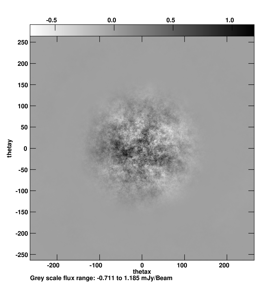
To simulate the diffuse emission, we mainly followed the same procedure as discussed in Choudhuri et al. (2014). We first create the Fourier components of the temperature fluctuations on a grid using
| (5) |
where is the total solid angle of the simulated area, and and are independent Gaussian random variables with zero mean and unit variance. Then, we use the Fastest Fourier Transform in the West (hereafter FFTW) algorithm (Frigo et al., 2005) to convert to , the brightness temperature fluctuations or equivalently the intensity fluctuations on the grid. The intensity fluctuations can be calculated using the Raleigh-Jeans approximation which is valid at the frequency of our interest. Figure 17 shows one realization of the intensity fluctuations map at the central frequency with and without multiplication of the GMRT primary beam. The multiplication of the primary beam with intensity fluctuations in the sky plane is equivalent to the convolution of the Fourier transform of the both quantities in the plane. The recovered angular power spectrum is affected due to the convolution of the primary beam only at large angular scales (). This affect has been shown already in Figure 3 of Choudhuri et al. (2014). Based on a large number of realizations of the simulated diffuse intensity map, we find that the estimated angular power spectrum without multiplication of PB is in good agreement with the input model power spectrum (eq. 23) at the scales of our interest .
Finally, we generate the specific intensity fluctuations at any other frequency in the observation frequency band from that of the reference frequency using the scaling relation
| (6) |
In general, the spectral index of the diffuse emission may have a spatial variation and the synchrotron power spectrum may be different at different frequencies. However, the effect of this on point source subtraction is expected to be negligible, and the final results do not depend on the constancy of the synchrotron power spectrum slope. Here, we assume that the value of is fixed over the whole region and across the observation band in the multi-frequency simulation.
2.3 Simulated GMRT Observation
The simulations are generated keeping realistic GMRT specifications in mind, though these parameters are quite general, and similar mock data for any other telescope can be generated easily. The GMRT has antennas. The diameter of each antenna is . The projected shortest baseline at the GMRT can be , and the longest baseline is . The instantaneous bandwidth is , divided into channels, centered at . We consider all antennas targeted on a arbitrary field located at R.A.= Dec= for a total of observation. The visibility integration time was chosen as . The mock observation produces samples per channels in the whole range. Each baseline generates visibilities because of spectral channels in the observation frequency-band. Figure 18 shows the full coverage at central frequency for the simulated GMRT Observation. Table 2 summarizes the GMRT parameters used in this work.
The angular power spectrum of the diffuse synchrotron emission (eq. 23) declines with increasing baseline (), and drops significantly at the available longest baseline. Hence, for our simulation, the contributions of the diffuse emission have been taken from only baselines to reduce the computation time. To calculate the visibilities, we multiply the simulated intensity fluctuations with the PB (eq. 30), and we use 2-D FFTW of the product in a grid. For each sampled baseline , we interpolate the gridded visibilities to the nearest baseline of the track in Figure 18. We notice that the -term does not have significant impact on the estimated angular power spectrum of diffuse synchrotron emission (Choudhuri et al., 2014). But, to make the image properly and also to reduce the point source sidelobes, it is necessary to retain the -term information. The -term also improves the dynamic range of the image and enhances the precision of point source subtraction. We use the full baseline range to calculate the contribution from the point sources. The sky model for the point sources is multiplied with PB before calculating the visibilities. Using the small field of view approximation, the visibilities for point sources are computed at each baseline by incorporating the term:
| (7) |

| Parameter | Value (GMRT) |
|---|---|
| per channel | |
The system noise of the interferometer is considered to be independent at different baselines and channels, and is modelled as Gaussian random variable. We add independent Gaussian random noise to both the real and imaginary parts of each visibility contribution. For a single polarization, the rms noise in the real or imaginary part of a visibility is predicted to be (Thompson, Moran & Swenson, 1986),
| (8) |
where is the total system temperature, is the Boltzmann constant, is the effective collecting area of each antenna, is the channel width and is correlator integration time. For a channel width of and integration time , the rms noise comes out to be for GMRT at single polarization. The two polarizations are assumed to have identical sky signals but independent noise contribution.
In summary, our simulated visibilities for the GMRT observation are sum of two independent components namely the sky signal and the system noise. As outlined above, the realistic sky signal contains the contribution of the extragalactic point sources and the diffuse synchrotron emission from our own Galaxy. The visibility data does not contain any calibration errors, ionospheric effects and radio-frequency interference (RFI). We leave a detailed investigation of these effects for future work.
3 Data Analysis


The simulated visibility data described above is generated using sky emission model containing a combination of point sources and Galactic diffuse synchrotron emission (along with instrumental noise). Our next goal is to analyse these simulated data to recover the statistical properties of the diffuse emission, and compare those with the known input model parameters. As mentioned earlier, to estimate the power spectrum of the diffuse emission, our approach is to first remove the point source foreground accurately. This requires imaging and deconvolution to model the point sources, and then subtracting them from the data. In reality, there are many issues which make an accurate subtraction of point sources from radio interferometric wide-field synthesis images challenging. These include residual gain calibration errors (Datta et al., 2009; Datta et al., 2010), direction dependence of the calibration due to instrumental or ionospheric/atmospheric conditions (Intema et al., 2009a; Yatawatta, 2012), the effect of spectral index of the sources (Rau & Cornwell, 2011), frequency dependence and asymmetry of the primary beam response, varying point spread function (synthesized beam) of the telescope (Bowman et al., 2009; Liu et al., 2009a; Morales et al., 2012; Ghosh et al., 2012), high computational expenses of imaging a large field of view, and CLEANing a large number of point sources (Pindor et al., 2011, particularly severe at low radio frequency (e.g. ) images,) etc. Earlier, Datta et al. (2009); Datta et al. (2010) have studied the effect of calibration errors in bright point source subtraction. They have concluded that, to detect the EoR signal, sources brighter than should be subtracted with a positional accuracy better than 0.1 arcsec if calibration errors remain correlated for a minimum time 6 hours of observation. The polarized galactic synchrotron emission is expected to be Faraday-rotated along the path, and it may acquire additional spectral structure through polarization leakage at the telescope. This is a potential complication for detecting the HI signal (Jelic et al., 2010; Moore et al., 2013). To cope with the capabilities of current and forthcoming radio telescopes, recently there have been a significant progress in developing calibration, imaging and deconvolution algorithms (Bhatnagar et al., 2013; Cornwell et al., 2008) which can now handle some of the above-mentioned complications.
In this paper, we take up a study of the effect of incomplete spectral modeling and of different deconvolution strategies to model and subtract point sources using simulated data at . The power spectrum estimator that we have used takes care of, at least to a large extent, issues like asymmetry of the primary beam, direction dependence of the calibration for the outer region of the field of view and high computational expenses of imaging and removing point sources from a large field of view etc. We leave studying the other calibration related issues for future work.
For our analysis, we use the Common Astronomy Software Applications (CASA) *‡*‡ *‡ http://http://casa.nrao.edu/ to produce the sky images from the simulated visibility data. To make a CLEAN intensity image, we use the Cotton-Schwab CLEANing algorithm (Schwab, 1984) with Briggs weighting and robust parameter 0.5, and with different CLEANing thresholds and CLEANing boxes around point sources. The CLEANing is done also with or without multifrequency synthesis (MFS; Sault & Wieringa 1994; Conway et al. 1990; Rau & Cornwell 2011). During deconvolution, MFS, if used, takes into account the spectral variation of the point sources using Taylor series coefficients as spectral basis functions. In a recent paper Offringa et al. (2016) suggest that CASA’s MS-MFS algorithm can be used for better spectral modelling of the point sources. The large field of view () of the GMRT at lead to significant amount of errors if the non-planar nature of the GMRT antenna distribution is not taken into account. For this purpose we use projection algorithm (Cornwell et al., 2008) implemented in CLEAN task within the CASA. For different CLEANing strategies, we assess the impact of point sources removal in recovering the input angular power spectrum of diffuse Galactic synchrotron emission from residual data. Effectively, by CLEANing with these different options, we identify the optimum approach to produce the best model for point source subtraction and estimation. We investigate the CLEANing effects both in the image domain by directly inspecting the “residual images” after the point source subtraction, and also in the Fourier domain by comparing the power spectrum of the residual data with the input power spectrum of the simulated diffuse emission. For discussion on some of the relevant methods and an outline of the power spectrum estimation, please see Choudhuri et al. (2014) and references therein.
The left panel of Figure 19 shows the resultant CLEANed image of the simulated sky of the target field with angular size . The synthesized beam has a . The image, as mentioned earlier, contains two different emission components (i.e. point sources, diffuse synchrotron emission) and noise. The grey scale flux density range in Figure 19 is saturated at to clearly show the diffuse emission. The inner part () of CLEANed image has rms noise , and it drops to at the outer part of the image where the response of the GMRT primary beam attenuates quite a bit compared to the phase centre. In the right panel of Figure 19, we also show a small portion (marked as a square box in the left panel) of the image with an angular size . We note that there is a strong point source at the centre of this small image with a flux density of and spectral index of . The intensity fluctuations of the diffuse emission are also clearly visible in both the panels of Figure 19.
Figure 20 shows the angular power spectrum estimated from the simulated visibilities before any point source subtraction. We find that the estimated power spectrum, as expected, is almost flat across all angular scales. This is the Poisson contribution from the randomly distributed point sources which dominate at all angular multipoles in our simulation. In this paper, we do not include the clustering component of the point sources which becomes dominant only at large angular scales () (Ali et al., 2008) where it introduces a power law dependence in the angular power spectrum. We also note that the convolution with the primary beam affects the estimated angular power spectrum at small values (Figure 3, Choudhuri et al. 2014), and it will be difficult to individually distinguish the Poisson and the clustered part of the point source components with the GMRT. The total simulated power spectrum (Figure 20) is consistent with the previous GMRT observations (Ali et al. 2008; Ghosh et al. 2012). In Figure 20 we also show the input model angular power spectrum of the diffuse emission along with 1- error bar (shaded region) estimated from 100 realizations of the diffuse emission map. Note that the angular power spectrum of the diffuse emission is buried deep under the point source contribution which dominates at all the angular scales accessible to the GMRT. We would like to emphasis that, in this paper, our aim is to study how well we can recover this diffuse power spectrum from the residual visibility data after point source subtraction is carried out to the desired level.
It is quite difficult to model and subtract out the point sources from the sidelobes and the outer parts of the main lobe of the primary beam. Our recent paper (Choudhuri et al., 2016a) contains a detailed discussion of the real life problems for modelling and subtracting point sources from these regions. In this paper we have restricted the point source subtraction to the central region of the primary beam (as detailed in the next section). Here we have used the TGE to estimate the angular power spectrum from the visibilities (both before and after point source subtraction). The TGE tapers the sky response to suppress the effect of the point sources outside the FWHM of the primary beam. This is achieved by convolving the visibilities with a window function whose width can be varied. It is also devised in such a way that it calculates the noise bias internally, and subtracts its contribution to extract only the desired signal. The TGE is an unbiased estimator for the angular power spectrum , and a detailed description has been presented in our earlier paper (Choudhuri et al., 2014). Here we have applied the TGE to the simulated visibility data to estimate in logarithmic intervals of after averaging all the frequency channels. The same estimator may also be extended to quantify the cosmological signal, we plan to address this in future.

4 Point Source Subtraction
The bright discrete point sources are the most dominant foreground component for detecting the redshifted HI 21-cm EoR signal. As shown in (Figure 20), the radio sky is dominated by them at the angular scales (Ali et al., 2008). Therefore, it is very crucial to identify all point sources precisely from the image, and remove their contribution from the visibility data in order to estimate the power spectrum of background diffuse emission. In this section, we discuss the point source modeling and the effect of different CLEANing strategies on the “residual” images, made from the point source subtracted visibility data.
We use different sets of parameter shown in Table 3 for different CLEANing strategies. Pixels with flux density above a threshold value in the image are identified as point sources which are used to build the “clean component” model. The model visibilities corresponding to these clean components are subtracted from the original multi-frequency data using the standard CASA task UVSUB. This should remove the point source contribution from the data to a large extent. The residual images, hence, are expected to be dominated by the diffuse emissions and the system noise. After point source subtraction we make residual images of size . Figure 21 shows a representative region of angular size , to illustrate the effect of different cleaning schemes. The different residual images (Image(a) to Image(f)) in Figure 21 correspond to the different CLEANing strategies in Table 3 (Run(a) to Run(f)).
First we investigate the effect of spectral modelling of the clean components in the residual image. This is done by changing the parameter “nterms” where nterms=1 does not include any spectral correction, while nterms=2 builds the model by including spectral index during multi-frequency CLEANing. A more detailed discussions of these parameters can be found in Rau & Cornwell (2011). For point source subtraction with a CLEANing threshold of and and , the “dirty” images of the residual UVSUB data are shown in Figure 21 top row (left and right panel for and respectively). The strong sidelobe patterns appear around the central bright source in Image(a) for incorrect spectral modelling. Most of these disappear in Image(b) where the spectral property of the bright source has been taken into account during CLEANing and continuum subtraction.
In the middle row of Figure 21, we compare the residual images for two different CLEANing threshold and (left and right panel respectively) while keeping fixed for both. We notice that for the CLEANing threshold of , part of the diffuse structure is also CLEANed and subtracted out form the data. On the other hand, all the diffuse structures (but also some residual from the point sources) are still present in the residual Image(d) where we use a higher threshold of (). The overlayed contours in Figure 21 make the comparison more clear. For the panels in the top and the middle row, we CLEANed the whole image upto the specified threshold without making any CLEAN box around the point sources. This is more computation expensive as well as inadequate to handle the diffuse structure, and will remove positive and negative peaks of the diffuse signal. For EoR experiments, a part of the desired diffuse signal, if present, may also be removed by such deep CLEANing without making boxes.
| Name | nterms | Threshold flux density | CLEANing Box |
|---|---|---|---|
| Run(a) | 1.0 mJy | Single Box | |
| Run(b) | 1.0 mJy | Single Box | |
| Run(c) | 0.5 mJy | Single Box | |
| Run(d) | 2.0 mJy | Single Box | |
| Run(e) | 0.5 mJy | Circular region with radius | |
| around all sources in the image | |||
| Run(f) | 2.0 mJy | Single Box | |
| 0.5 mJy | Box around | ||
| each visible residual sources |


Next we use CLEAN boxes to create the model for point source subtraction. This will ensure that the clean components are picked up only from the restricted regions defined by the shape of the box as highlighted in the bottom row of Figure 21. Here, we select the boxes in two ways (see Table 3). In the first case, we use the mask file (circular box of radius ) from the catalogue sources which are used to generate the simulated data, and CLEANed upto threshold. For the second case, we first CLEANed the whole image upto a conservative limit of . Then, by visually inspecting the image, we identified residual point sources which are not cleaned due to higher threshold, and placed rectangular boxes of size around each of them. These selected regions are then CLEANed upto a limit of . The residual images for these two cases are shown in the bottom row of Figure 21 (Image(e) and Image(f)). We notice that there is no significant difference in the residuals for these two cases. In the next section, we assess impact of the different CLEAN strategies on the statistics such as distribution of visibilities and estimated angular power spectrum from different residual data sets.
5 Results


We use different CLEANing strategies to subtract point sources from a region of the sky from simulated visibility data discussed in Section 4. To compare the outcome of these strategies, we check the statistics of the visibilities as well as of the images. In Figure 22 we show the normalized histogram plots from images (top row) and from the visibility data (bottom row). First we consider the CLEANed and the residual images. The top-left panel of Figure 22 shows the distribution of the pixel values from the initial CLEANed map (Figure 19). This plot shows a small number of pixels with high flux density values (due to the bright point sources). The distribution is, however, dominated by the diffuse foreground component with relatively small values () over a large fraction of pixels. The top-middle and right panel show the histogram of the residual images from different CLEANing runs discussed in Section 4. A Gaussian with is a fairly good fit to the distribution of the residuals upto a flux density limit of . However, as evident from the top central panel, CLEANing with lower threshold (see Table 3) makes residual images more non-Gaussian. The histogram for Run(c), for example, is confined to lower flux density range, because “blind” CLEANing with very low threshold removes a part of diffuse structure. In the top right panel, we show the impact of choosing CLEAN boxes in different ways (Run(e) and (f) in Table 3), keeping a fixed threshold flux density of . We find that there is no difference in the distribution of the residual images for Run(e) and Run(f). Also, in all the cases, they follow the same Gaussian function upto .
Next, we consider the statistics of the visibilities. The corresponding visibility distribution functions are shown in the bottom row of Figure 22. We use the real part the complex visibilities for the purpose of this comparison in the plots, but the imaginary parts also have a similar distribution. We find that the initial and residual visibility data both mostly follow a Gaussian distribution, but with different standard deviation. The initial visibility data (bottom row, left panel of Figure 22) follows a Gaussian distribution with Jy. The residual visibility data, however, can be fitted with a Gaussian function of Jy upto a flux density limit of containing the bulk of the data. The counts significantly deviate from a Gaussian at large visibility values most likely due to incomplete CLEANing.
The angular power spectrum have been estimated from the residual visibility data with the different CLEANing strategies. As mentioned earlier, this estimation is done using TGE. Here, we have used Gaussian window function to taper the sky response. The tapering is introduced through a parameter , where is preferably so that modified window function inside the TGE cuts off the sky response well before the first null of the primary beam (see for details, Figure 1 of Choudhuri et al. 2016a). The reduced field of view results in a larger cosmic variance for the angular modes which are within the tapered field of view. So, the tapering parameter will possibly be determined by optimizing between the reduced field of view and the cosmic variance. In this work we use . It is expected that the estimated power spectrum from the residual data will be consistent with the input power spectrum if the point source subtraction is perfect and precise. Through angular power spectrum estimation from the different residual data sets, we try to find out the optimum approach for CLEANing to recover the underlying diffuse synchrotron emission power spectrum. Figure 23 shows the estimated from the residual visibility data for Run(a) and Run(b), that is for fixed CLEANing threshold of but and respectively. We note that the residual sidelobes around the bright sources in the image with (see Figure 21a) introduced an excess power at large angular multipoles (small angular scales) in the estimated angular power spectrum. On the other hand CLEANing with reduces the residual sidelobes in the image after point source subtraction (see Figure 21b). Hence, in this case the estimated , as shown in Figure 23, recover the input power spectrum better at large values as well.
Figure 24 shows the angular power spectra estimated from the residual visibility data obtained under the different CLEANing strategies Run(b), Run(c) and Run(d) with different threshold but fixed value of (see Table 3). For Run(d), which cleans upto (), the angular power spectrum below is properly recovered. However, due to insufficient CLEANing, it retains some extra residual power at large . In contrast, as already noted earlier, Run(b) with CLEANing threshold of recovers the power spectrum for a larger range of . The estimated angular power spectrum for Run(c), on the other hand, falls off by a factor compared to the input model power spectrum at all angular scales. This is due to the fact that Run(c) removes a part of diffuse structure from the map by CLEANing upto .


The effect of using different CLEANing box options (discussed in Section 4) in recovering is shown in Figure 25. Here we keep the other two parameters fixed at and CLEANing threshold of . It is clear from this figure that there is no significant change in the estimated power spectra for the two different CLEANing box strategies used in Run(e) and (f). In both of these cases the estimated agree very well with the input power spectrum over the full range of probed here. For comparison, we also show the estimated power spectrum for Run(c) where the full image is CLEANed upto without selecting any CLEAN region around the point sources. As already shown, this partly removes the underlying diffuse emission from the image. Thus, the estimated in this case is a factor lower compared to the input model power spectrum at all angular scales.
6 Summary and conclusions
Precise subtraction of point sources from wide-field interferometric data is one of the primary challenges in studying the diffuse foreground emission as well as the weak redshifted HI 21-cm signal. In this paper, we consider the method of studying and characterizing the Galactic synchrotron emission using simulated GMRT observation in presence of point sources. The angular power spectrum of the diffuse emission is estimated from the residual visibility data using TGE after subtracting the point sources from only the inner part of the field of view of size . We assess the impact of imperfect point source removal for different CLEANing strategies in recovering both the flux density distribution and the input of the diffuse Galactic synchrotron emission for the angular scale range probed by the GMRT.
The simulations are carried out for GMRT observation for a sky model consisting of point sources and diffuse synchrotron emission. The sky model is multiplied with the model PB , before computing the visibilities for the frequency and the coverage of the simulated GMRT observation. Finally, we add independent Gaussian random noise to both the real and imaginary parts of each visibility contribution. The standard analysis package CASA has been used to make images and to subtract point source model from the simulated visibility data. We use various CLEANing strategies as outlined in Section 4 with different CLEANing boxes, threshold flux and spectral correction options. The residual data were then used for estimating of the diffuse component. We check the effect of point source subtraction by comparing image histograms, visibility distribution function as well as from the residual data.
We find that all the different CLEANing strategies introduce some degree of non-Gaussianity in the residual data both in image and in visibility domain. The less precise point source subtraction generates more non-Gaussianity in the distribution of image-pixels beyond the CLEANing threshold. Equivalently, the visibility distributions also deviate significantly from a Gaussian. Comparing the recovered and the input power spectra, we find that both shallow CLEANing and incorrect spectral modelling of the point sources leave artifacts in the residual image near the position of bright point sources, and also results in excess power at the large angular multipoles (). On the other hand, very deep “blind” CLEANing removes part of the diffuse structure and reduces the amplitude of the power spectrum at all angular scale. The best possible situation is when, for a given region, source catalogue is available from other observations (even at a different frequency). Naturally, the optimum option there is to use the existing source catalogue to choose CLEANing regions for deep CLEANing (with threshold ) along with spectral correction for the point source model ( or higher). If a point source catalogue is not available, then one may use a moderate CLEANing threshold () for the whole image (which may still remove some of the diffuse signal). Alternatively, one may use a more conservative initial CLEANing threshold () for the whole image, and then choose CLEANing box around residual sources by visual inspection for a deeper () CLEANing. The latter strategy is useful only when one needs to remove the point sources from a relatively smaller region. Please note that, for the TGE, effect of the residual point sources from the outer region of the field is insignificant due to the tapering. Hence, we need to accurately subtract point sources only from the inner region, which makes it a viable option in the present case. We find that both this strategy and deep CLEANing based on source catalogue give a comparably good estimation for these simulated data.
The accurate removal of all the point sources from the wide-field image is complicated and difficult task in presence of instrumental systematics, calibration errors, RFI and ionospheric effects. In absence of the mentioned real-world obstacles, we subtract out all the point sources from the image with high level of accuracy, and the TGE successfully recovers the angular power spectrum of diffuse Galactic synchrotron emission from the residual visibility data at the angular scales probed by the GMRT. As a next step, we plan to incorporate some of the above mentioned “real world” observational effects in our simulation, and investigate how precisely we can remove the point sources and estimate the angular power spectrum from the residual data. We leave this issue for future studies.
Chapter 4 Tapering the sky response for angular power spectrum estimation from low-frequency radio-interferometric data*§*§ *§ This chapter is adapted from the paper “Tapering the sky response for angular power spectrum estimation from low-frequency radio-interferometric data” by Choudhuri et al. (2016a)
1 Introduction
Foreground removal for detecting the Epoch of Reionization (EoR) 21-cm signal is a topic of intense current research (Jelić et al., 2008; Bowman et al., 2009; Paciga et al., 2011; Chapman et al., 2012; Liu & Tegmark, 2012; Mao, 2012; Paciga et al., 2013). Foreground avoidance (Datta et al., 2010; Parsons et al., 2012; Trott et al., 2012; Vedantham et al., 2012; Pober et al., 2013; Thyagarajan et al., 2013; Parsons et al., 2014; Dillon et al., 2014; Pober et al., 2014; Liu et al., 2014a; Liu et al., 2014b; Ali et al., 2015) is an alternate strategy based on the proposal that the foreground contamination is restricted to a wedge in space, and the signal can be estimated from the uncontaminated modes outside the wedge. Point sources dominate the sky at the angular scales (Ali et al., 2008) which are relevant for telescopes like the Giant Metrewave Radio Telescope (Swarup et al., 1991, GMRT;), Low-Frequency Array (var Haarlem et al., 2013, LOFAR;) and the upcoming Square Kilometre Array (SKA). It is difficult to model and subtract the point sources at the periphery of the telescope’s field of view. The difficulties include the fact that the antenna response is highly frequency dependent near the nulls of the primary beam, and the calibration differs from that of the phase center due to ionospheric fluctuations. Point source subtraction is also important for measuring the angular power spectrum of the diffuse Galactic synchrotron radiation (Bernardi et al., 2009; Ghosh et al., 2012; Iacobelli et al., 2013) which, apart from being an important foreground component for the EoR 21-cm signal, is interesting in its own right.
Most of the foreground subtraction techniques use the property of smoothness along frequency for the various foreground components. Ghosh et al. (2011a); Ghosh et al. (2011b) found that residual point sources located away from the phase center introduce oscillations along frequency direction. The oscillation are more rapid if the distance of the source from the phase center increases, and also with increasing baseline. Equivalently, the dominant contribution to the width of the foreground wedge arises from the sources located at the periphery of the field of view (Thyagarajan et al., 2013). Using GMRT Ghosh et al. (2011b); Ghosh et al. (2012) have shown that these oscillations can be reduced by tapering the sky response. In a recent paper Pober et al. (2016) showed that correctly modelling and subtracting the sidelobe foreground contamination is important for detecting the redshifted 21-cm signal.
In a recent paper Choudhuri et al. (2014) have introduced the Tapered Gridded Estimator (TGE) for estimating the angular power spectrum directly from radio-interferometric visibility data. In this paper we use simulated GMRT data which incorporates point sources and the diffuse Galactic synchrotron radiation to demonstrate that it is possible to suppress the contribution from residual point sources in the sidelobes and the outer parts of the primary beam in estimating using the TGE.
Noise bias is an important issue for any estimator. For example, the image based estimator (Seljak, 1997) for and the visibility based estimator (Liu & Tegmark, 2012) for rely on modelling the noise properties of the data and subtracting out the expected noise bias. However, the actual noise in the observations could have baseline, frequency and time dependent variations which are very difficult to model and there is the risk of residual noise bias being mistaken as the signal. Paciga et al. (2011) have avoided the noise bias by cross-correlating observations made on different days. Another visibility based estimator (Begum et al., 2006; Dutta et al., 2008) individually correlates pairs of visibilities avoiding the self correlation that is responsible for the noise bias. This, however, is computationally very expensive when the data volume is large. In this paper, we have demonstrated that TGE, by construction, estimates the actual noise bias internally from the data and exactly subtracts this out to give an unbiased estimate of . The entire discussion here is in the context of estimating for the diffuse Galactic synchrotron radiation. As mentioned earlier, the same issues are also relevant for measuring the EoR 21-cm power spectrum not considered here.
In Section 2 we discuss the conventional problem in standard imaging techniques. Simulation and data analysis processes are briefly discussed in Section 4. Section 4 discusses the estimator (TGE) that we used to suppress the outer region of the primary beam and the results are presented in Section 5. Finally, we present summary and conclusion in Section 6.
2 Problems in conventional Imaging
The contribution to the signal in radio frequency observations from the outer region of the primary beam and from the sidelobes is generally very small as compared to the inner region of the primary beam. In particular, the expected 21-cm signal, which itself is very faint, contributes mainly from the central part of the primary beam, and attenuated to a great extent in the outer region. Only the bright point sources from the outer region, if not accurately removed, may have significant impact on the statistical estimation of the diffuse signal. Thus, it is necessary to remove the effect of point sources from the outer region before estimating the residual power spectrum. However, we will not be benefitted in terms of signal by including highly attenuated diffuse emission from the outer region.
Imaging a large enough region to model and subtract all the point sources before dealing with the diffuse emission may seems to be a direct solution of the above problem. But, in reality there are many issues which make this approach impractical. First of all, the field of view at low radio frequencies is large, and making larger images is computationally more expensive. In addition to that, non-coplaner nature of the baselines prevents us from making wide-field image without considering the effect of the “w-term”. There are algorithms e.g. faceting (Cornwell & Perley, 1992), w-projection (Cornwell et al., 2008), WB-A projection (Bhatnagar et al., 2013) etc. to tackle this problem partly for radio interferometric observations. However, these algorithms still require significant computation to make an image of such a large region of the sky. Secondly, the number of bright point sources is quite large at low frequency. While imaging a very large region, selecting CLEANing region around each source is a tedious job. On the other hand, CLEANing without selecting regions removes a non-negligible part of the diffuse signal of our interest (see Choudhuri et al., 2016c, for details).
The next challenge is to accurately characterize the time and frequency dependence of the wide-field primary beam for effective point source subtraction from the periphery of the telescope’s field of view (Neben et al., 2015, e.g.). Both the frequency dependence and the deviation from circular symmetry are more prominent at the outer part of the primary beam. These, along with the rotation of primary beam on the sky, cause a strong time and frequency variation of the primary beam for point sources in the outer region. They create problem in accurately model the point sources that we want to subtract from the data. In fact, some of the variations are intractable in nature and it is extremely difficult, if not impossible, to make accurate modelling and subtraction of the point sources from the outer part of the primary beam.
Though we have not considered instrumental gains and ionospheric effects in this study, in real life any directional dependence of these quantities will also severely limit our ability to subtract point sources accurately from a large region. One can overcome this difficulty to some extent by going into complicated and messy procedure of direction dependent calibration (e.g. peeling) (Bhatnagar et al., 2008; Intema et al., 2009a; Kazemi et al., 2011). Again, (a) it is computationally more expensive, (b) part of the variation may be intractable, and (c) there is hardly any gain in terms of recovering the diffuse signal which is too weak in outer region.
The future generation low frequency telescopes (e.g. SKA) that will presumably be used to carry out redshifted diffuse H i observation, will have larger field of view, large bandwidth, longer baseline and higher sensitivity. Hence the above issues will be even more relevant. Moreover, the expected huge data volume from observations with those telescopes will make it more challenging to address these problems by imaging a larger region for subtracting the point sources. The following two sections outline a technique to overcome these problems by subtracting point sources only from the central region and using the TGE to recover the power spectrum of the diffuse emission in a more efficient way.
3 Simulation and Data Analysis
The details of the simulation and data analysis, including point source subtraction, are presented in a companion paper (Choudhuri et al., 2016c) and we only present a brief discussion here. Our model of the sky has two components, the first being the diffuse Galactic synchrotron radiation which is the signal that we want to detect. We use the measured angular power spectrum (Ghosh et al., 2012)
| (1) |
as the input model to generate the brightness temperature fluctuations on the sky. Here is the frequency in , , (Ghosh et al., 2012) and (Platania et al., 1998). The simulation covers a region of the sky and a bandwidth, centered at , over spectral channels. The diffuse signal was simulated on a grid of resolution .
The Poisson fluctuation of the extragalactic point sources dominates the sky at the angular scales of our interest (Ali et al., 2008), and it is necessary to subtract these or suppress their contribution in order to detect any diffuse component like the Galactic synchrotron radiation which we consider here or the redshifted 21-cm cosmological signal which is much fainter and is not considered here. We use the differential source count measured using GMRT (Ghosh et al., 2012)
| (2) |
to generate point sources in the flux range to whose angular positions are randomly distributed within the Full Width Half Maxima (hereafter FWHM) of the primary beam. The antenna response falls off beyond the FWHM, and we only include the bright sources () outside the FWHM. We have and sources in the inner and outer regions respectively, and the sources were assigned a randomly chosen spectral index () in the range to .
We consider the mock GMRT observations targeted on a arbitrarily selected field located at RA= and DEC=. The GMRT has antennas which for a total of observation with integration time results in baselines with visibilities (one per frequency channel) for each baseline. The resolution of GMRT at is . The diffuse signal (eq. 23) falls off with increasing (), and we include this contribution for only the small baselines for which the visibility contribution is calculated using a 2 dimensional Fourier transform. We note that the term does not significantly affect the diffuse signal (Choudhuri et al., 2014), however this is very important for correctly imaging and subtracting the point sources. We have included the point source contribution for all the baselines in the simulation, and the visibilities are calculated by individually summing over each point source and including the term. We have modelled the GMRT primary beam pattern with the square of a Bessel function (Figure 26) corresponding to the telescope’s diameter circular aperture. The simulated sky is multiplied with before calculating the visibilities. Finally, we add the system noise contribution which is modelled a Gaussian random variable with standard deviation for the real and imaginary parts of each visibility. We note that the GMRT has two polarizations which have identical sky signals but independent noise.

We have used the Common Astronomy Software Applications (CASA) package to image and analyze our simulated data. The standard tasks CLEAN and UVSUB were used to model and subtract out the point sources from a region which covers an extent that is approximately times the FWHM of the primary beam. We have tried different CLEAN strategies for which the details are presented in our companion paper (Choudhuri et al., 2016c), and for this work we adopt the most optimum parameter values which correspond to Run(e) of the companion paper. Figure 27 shows the “dirty” image of the entire simulation region made from the residual visibility data after point source subtraction. The central square box () shows the region from which the point sources have been subtracted. The features visible in this region correspond to the Galactic synchrotron radiation. It is difficult to model and subtract point sources from the periphery where the antenna response is highly frequency dependent. It also needs creating and cleaning a huge image that is computationally more expensive. Further, in real observations, any direction dependent gain away from the phase center will make it even more difficult. We have not attempted to subtract the point sources from the region outside the central box and the residual point sources are visible in this region of the image.
Figure 28 shows the angular power spectrum before and after point source subtraction; the input model for the diffuse radiation is also shown for comparison. Before subtraction, the point sources dominate at all angular multipoles . After subtraction, we are able to recover the diffuse component at low angular multipoles . However, the residual point sources still dominate at the large values. The goal is to suppress the contribution from the residual point sources located at the periphery of the beam so that we can recover the input model over the entire range. We show that it is possible to achieve this with the Tapered Gridded Estimator discussed in the next section.

4 The Tapered Gridded Estimator
The observed visibilities are a sum of two independent parts namely the sky signal and the system noise
| (3) |
The signal and the noise are considered to be independent random variables, further the noise in the different visibilities are uncorrelated. The signal contribution records the Fourier transform of the product of , the fluctuation in specific intensity of the sky signal, and the telescope’s primary beam pattern shown in Figure 26. As mentioned earlier, it is difficult to model and subtract point sources from the outer region of the primary beam and the sidelobes. The residual point sources in the periphery of the telescope’s field of view pose a problem for estimating the power spectrum of the diffuse radiation. In this section we discuss the Tapered Gridded Estimator (TGE) which is a technique for estimating the angular power spectrum from the visibility data. This technique suppresses the contribution from the sidelobes and the outer part of the primary beam by tapering the sky response. Choudhuri et al. (2014) presents a detailed discussion of this estimator, and we only present a brief outline here.
We taper the sky response by multiplying the field of view with a frequency independent Gaussian window function . Here we parameterize where and is the FWHM of the telescope’s primary beam at the central frequency, and preferably so that cuts off the sky response well before the first null of the primary beam. We implement the tapering by convolving the measured visibilities with the Fourier transform of . The convolved visibilities are evaluated on a grid in space using
| (4) |
where refers to the different grid points and refers to the measured visibilities at baseline . The gridding significantly reduces the data volume and the computation time required to estimate the power spectrum (Choudhuri et al., 2014). The convolved visibilities are calculated separately for each frequency channel. Then, for the purpose of this work, convolved visibilities for a grid are averaged over all frequencies.
The signal component of the convolved visibility is the Fourier transform of the product of a modified primary beam pattern and
| (5) |
It is clear that the convolved visibilities respond to the signal from a smaller region of the sky as compared to the measured visibilities. It may be noted that the tapering is effective only if the window function in eq. (54) is well sampled by the baseline distribution. The results of this paper, presented later, indeed justify this assumption for the GMRT.
The correlation of the gridded visibilities gives a direct estimate of the angular power spectrum through
| (6) |
where the angular multipole is related to the baseline as , , , is the Fourier transform of and is the conversion factor from brightness temperature to specific intensity. We see that the visibility correlation also has a term involving which is the variance of the noise contribution present in the measured visibilities (eq. 47). This term, which is independent of , introduces a positive definite noise bias. The visibility correlation (eq. 6) provides an estimate of except for the additive noise bias. The TGE uses the same visibility data to obtain an internal estimate of the noise bias and subtract it from the visibility correlation. We consider the self-correlation term for which
| (7) |
where , is the Fourier transform of the primary beam pattern . The term , by construction, has exactly the same noise bias as the visibility correlation in eq. (6). We use this to define the TGE estimator
| (8) |
which gives an unbiased estimate of the angular power spectrum at a grid point . A part of the signal also gets subtracted out with the noise bias. This loss is proportional to (the number of visibility data) whereas the visibility correlation is proportional to , and this loss is insignificant when the data size is large (Choudhuri et al., 2014). The values estimated at each grid point are binned in logarithmic intervals of , and we consider the bin-averaged as a function of the bin-averaged angular multipole .
Tapering reduces the sky coverage which, in addition to suppressing the point sources in the periphery of the main lobe and the sidelobes, also affects the diffuse signal. The reduced sky coverage causes the cosmic variance of the estimated to increase as is reduced (Figure 10, Choudhuri et al. 2014). Further, the reduced sky coverage also restricts the range () where it is possible to estimate , and the value of increases as is decreased.
5 Results
We have applied the Tapered Gridded Estimator (TGE) to the residual visibility data after subtracting out the point sources. As mentioned earlier, the point sources have been identified and subtracted from a region (Figure 27) which covers an extent that is times the FWHM of the primary beam. However, the point sources still remain at the periphery of the primary beam and in the part of the sidelobe which has been included in the simulation. The TGE tapers the sky response which results in an effective primary beam that is considerably narrower than the actual primary beam of the telescope . Figure 26 shows for three different values of ( and ). For we see that is not very significantly different from in the region within the first null, the difference however increases in the first sidelobe and the sidelobe response is suppressed by a factor of at . We see that the effective primary beam gets narrower as the value of is reduced. The value of is a factor of () lower compared to for () at which corresponds to the boundary of the region within which the point sources have been subtracted. We see that, for (), tapering suppresses the first side lobe of by a factor of () compared to at . We expect the residual point source contribution to reduce by at least a factor of and for and respectively.

Figure 28 shows the angular power spectrum () estimated from the residual visibility data using TGE with the values ( and ) discussed earlier. We see that in the absence of tapering we are able to recover the angular power spectrum of the diffuse synchrotron radiation at the low angular multipoles (large angular scales) . The residual point source contribution is nearly independent of and has a value which dominates the estimated at the large angular multipoles (small angular scales) . We have a gradual transition from the diffuse synchrotron dominated to a point source dominated in the interval . The point source contribution comes down by a factor of more than if we use the TGE with . We are now able to recover the angular power spectrum of the diffuse synchrotron radiation to larger values () as compared to the situation without tapering. The point source contribution, however, still dominates at larger values. We find that the point source contribution to is suppressed by more than a factor of if we use TGE with or . We are able to recover the angular power spectrum of the diffuse synchrotron radiation over the entire range using either value of . The fact that there is no noticeable change in if the value of is reduced from to indicates that a tapered sky response with is adequate to detect the angular power spectrum of the diffuse synchrotron radiation over the entire range of our interest here.
The noise bias is an important issue in estimating the angular power spectrum, we illustrate this in Figure 29. For this purpose we have used a smaller frequency bandwidth of which increases the noise r.m.s. compared to the bandwidth used throughout the rest of the paper. Figure 29 shows estimated with the TGE with . We expect to recover the angular power spectrum of the diffuse synchrotron radiation over the entire range provided the noise bias is correctly estimated and subtracted out. Figure 29 shows the estimated in the situation where the noise bias is not subtracted. We see that the noise bias makes a nearly constant contribution of which dominates the estimated at large . It is necessary to subtract the noise bias in order to recover the of the diffuse radiation at large . Figure 29 demonstrates that the TGE correctly subtracts out the noise bias so that we are able to recover the of the diffuse radiation over the entire range.

6 Summary and Conclusion
It is difficult to model and subtract point sources located at the periphery of the telescope’s field of view. These residual point sources pose a problem for estimating the power spectrum of the diffuse background radiation if all visible point sources are removed with high level of accuracy from inside the main lobe of the primary beam. For example, Pober et al. (2016) have recently shown the effect of the residual point sources outside the main lobe on estimating the power spectrum for MWA observation. This issue is discussed here in the context of measuring the angular power spectrum of the diffuse Galactic synchrotron radiation using simulated GMRT observations. However, the same issue is also very important for detecting the EoR 21-cm power spectrum which is a much fainter diffuse signal that is not considered here.
It is possible to suppress the contribution from the residual point sources located at the periphery of the telescope’s field of view through a frequency independent window function which restricts or tapers the sky response. The Tapered Gridded Estimator(TGE) achieves this tapering by convolving the measured visibilities with the Fourier transform of the window function. This estimator for the angular power spectrum has the added advantage that it internally estimates the noise bias from the measured visibilities and accurately subtracts this out to provide an unbiased estimate of . In this paper we demonstrate, using simulated data, that the TGE very effectively suppresses the contribution of the residual point sources located at the periphery of the telescope’s field of view. We also demonstrates that the TGE correctly estimates the noise bias from the input visibilities and subtracts this out to give an unbiased estimate of .
The issues considered here are particularly important in the context of measuring the EoR 21-cm power spectrum. While all the different frequencies have been collapsed for the present analysis, it is necessary to consider the multi-frequency angular power spectrum or equivalently the three dimensional power spectrum to quantify the 21-cm signal. We plan to generalize the TGE for this context in future work.
Chapter 5 The visibility based Tapered Gridded Estimator (TGE) for the redshifted 21-cm power spectrum*¶*¶ *¶ This chapter is adapted from the paper “The visibility based Tapered Gridded Estimator (TGE) for the redshifted 21-cm power spectrum” by Choudhuri et al. (2016b)
1 Introduction
Observations of the redshifted neutral hydrogen (HI) 21-cm radiation hold the potential of probing a wide range of cosmological and astrophysical phenomena over a large redshift range (Bharadwaj & Ali, 2005; Furlanetto et al., 2006; Morales & Wyithe, 2010; Pritchard & Loeb, 2012; Mellema et al., 2013). There now are several ongoing experiments such as the Donald C. Backer Precision Array to Probe the Epoch of Reionization (PAPER, Parsons et al. 2010), the Low Frequency Array (LOFAR, var Haarlem et al. 2013; Yatawatta et al. 2013) and the Murchison Wide-field Array (MWA, Bowman et al. 2013; Tingay et al. 2013) which aim to measure the power spectrum of the 21-cm radiation from the Epoch of Reionization (EoR, ). Future telescopes like the Square Kilometer Array (SKA1 LOW, Koopmans et al. 2015) and the Hydrogen Epoch of Reionization Array (HERA, Neben et al. 2016) are planned to achieve even higher sensitivity for measuring the EoR 21-cm power spectrum. Several other upcoming experiments like the Ooty Wide Field Array (OWFA; Prasad & Subrahmanya 2011; Ali & Bharadwaj 2014), the Canadian Hydrogen Intensity Mapping Experiment (CHIME*∥*∥ *∥ http://chime.phas.ubc.ca/; Bandura et al. 2014), the Baryon Acoustic Oscillation Broadband, Broad Beam Array (BAOBAB****** *** http://bao.berkeley.edu/; Pober et al. 2013a) and the Square Kilometre Array (SKA1 MID; Bull et al. 2015) target the post-Reionization 21-cm signal ().
Despite the sensitive new instruments, the main challenge still arises from the fact that the cosmological 21-cm signal is buried in astrophysical foregrounds which are orders of magnitude brighter (Shaver et al., 1999; Di Matteo et al., 2002; Santos et al., 2005; Ali et al., 2008; Paciga et al., 2011; Ghosh et al., 2011a; Ghosh et al., 2011b). A large variety of techniques have been proposed to overcome this problem and estimate the 21-cm power spectrum. The different approaches may be broadly divided into two classes (1.) Foreground Removal, and (2.) Foreground Avoidance.
The idea in Foreground Removal is to model the foregrounds and subtract these out either directly from the data (eg. Ali et al. 2008) or from the power spectrum estimator after correlating the data (eg. Ghosh et al. 2011a; Ghosh et al. 2011b). Foreground Removal is a topic of intense current research (Jelić et al., 2008; Bowman et al., 2009; Paciga et al., 2011; Chapman et al., 2012; Parsons et al., 2012; Liu & Tegmark, 2012; Trott et al., 2012; Pober et al., 2013; Paciga et al., 2013; Parsons et al., 2014; Trott et al., 2016).
Various studies (eg. Datta et al. 2010) show that the foreground contribution to the Cylindrical Power Spectrum is expected to be restricted within a wedge in the two dimensional (2D) plane. The idea in Foreground Avoidance is to avoid the Fourier modes within the foreground wedge and only use the uncontaminated modes outside the wedge to estimate the 21-cm power spectrum (Vedantham et al., 2012; Thyagarajan et al., 2013; Pober et al., 2014; Liu et al., 2014a; Liu et al., 2014b; Dillon et al., 2014; Dillon et al., 2015; Ali et al., 2015). In a recent paper Jacobs et al. (2016) have compared several power spectrum estimation techniques in the context of MWA.
Point sources dominate the low frequency sky at the angular scales (Ali et al., 2008) which are relevant for EoR 21-cm power spectrum with the telescopes like the GMRT, LOFAR and the upcoming SKA. It is difficult to model and subtract the point sources which are located at the periphery of the telescope’s field of view (FoV). The antenna response deviates from circular symmetry, and is highly frequency and time dependent at the outer parts of the telescope’s FoV. The calibration also differs from the phase center due to ionospheric fluctuations. The residual point sources located far away from the phase centre cause the signal to oscillates along the frequency direction (Ghosh et al., 2011a; Ghosh et al., 2011b). This poses a severe problem for foreground removal techniques which assume a smooth behavior of the signal along the frequency direction. Equivalently, these distant point sources reduce the EoR window by increasing the area under the foreground wedge in space (Thyagarajan et al., 2015). In a recent paper, Pober et al. (2016) showed that correctly modelling and subtracting the distant point sources are important for detecting the redshifted 21-cm signal. Point source subtraction is also important for measuring the angular power spectrum of the diffuse Galactic synchrotron radiation (Bernardi et al., 2009; Ghosh et al., 2012; Iacobelli et al., 2013). Apart from being an important foreground component for the EoR 21-cm signal, this is also interesting in its own right.
It is possible to suppress the contribution from the outer parts of the telescope’s FoV by tapering the sky response through a suitably chosen window function. Ghosh et al. (2011b) have analyzed GMRT data to show that it is possible to implement the tapering by convolving the observed visibilities with the Fourier transform of the window function. It is found that this reduces the amplitude of the oscillation along the frequency direction. Our earlier work Choudhuri et al. (2014) (hereafter Paper I) has introduced the Tapered Gridded Estimator (TGE) which places the findings of Ghosh et al. (2011b) on a sound theoretical footing. Considering observations at a single frequency, the TGE estimates the angular power spectrum of the 2D sky signal directly from the measured visibilities while simultaneously tapering the sky response. As a test-bed for the TGE, Paper I considers a situation where the point sources have been identified and subtracted out so that the residual visibilities are dominated by the Galactic synchrotron radiation. This has been used to investigate how well the TGE is able to recover the angular power spectrum of the input model used to simulate the Galactic synchrotron emission at . While most of the analysis was for the GMRT, simulations for LOFAR were also considered. These investigations show that the TGE is able to recover the input model to a high level of precision provided the baselines have a uniform coverage. For the GMRT, which has a patchy coverage, the is slightly overestimated using TGE though the excess is largely within the errors. This deviation is found to be reduced in a situation with a more uniform and denser baseline distribution , like LOFAR. Paper I also analyzes the effects of gain errors and the -term.
In a recent paper Choudhuri et al. (2016a) (hereafter Paper II) we have further developed the simulations of Paper I to include the point sources. We have used conventional radio astronomical techniques to model and subtract the point sources from the central region of the primary beam. As detailed in Paper II, it is difficult to do the same for the sources which are far away from the phase center, and these persist as residuals in the visibility data. We find that these residual point sources dominate the estimated at large baselines. We also show that it is possible to suppress the contribution from these residual sources located at the periphery of the FoV by using TGE with a suitably chosen window function.
Removing the noise bias is an important issue for any power spectrum estimator. As demonstrated in Paper II, the TGE internally estimates the actual noise bias from the data and subtracts this out to give an unbiased estimate of the power spectrum.
In the present work we report the progress on two counts. First, our earlier implementation of the TGE assumed a uniform and dense baseline coverage to calculate the normalization coefficient which relates visibility correlations to the estimated angular power spectrum . We, however, found (Paper I) that this leads to an overestimate of for instruments like the GMRT which have a sparse and patchy coverage. In Section 2 of this paper we present an improved TGE which overcomes this problem by using simulations to estimate the normalization coefficient. Second, the entire analysis of Papers I and II has been restricted to observations at a single frequency wherein the relevant issue is to quantify the 2D angular fluctuations of the sky signal. This, however, is inadequate for the three dimensional (3D) redshifted HI 21-cm signal where it is necessary to also simultaneously quantify the fluctuations along the frequency direction. In Section 3 of this paper we have generalized the TGE to quantify the 3D 21-cm signal and estimate the spatial power spectrum of the 21-cm brightness temperature fluctuations . We discuss two different binning schemes which respectively yield the spherically-averaged (1D) power spectrum and the cylindrically-averaged (2D) power spectrum , and present theoretical expressions for predicting the expected variance. We have validated the estimator and its variance predictions using simulations which are described in Section 4 and for which the results are presented in Section 5. Sections 6 presents the summary and conclusions.
In this paper, we have used cosmological parameters from the (Planck + WMAP) best-fit CDM cosmology (Planck Collaboration, P. A. R. Ade et al. 2015).
2 estimation
2.1 An Improved TGE
In this section we restrict our attention to a single frequency channel which we do not show explicitly in any of the subsequent equations. The measured visibilities can be decomposed into two contributions,
| (1) |
the sky signal and system noise respectively, and is the baseline corresponding to the -th visibility. The signal contribution records the Fourier transform of the product of the telescope’s primary beam pattern and the specific intensity fluctuation on the sky . Expressing the signal in terms of brightness temperature fluctuations we have
| (2) |
where is the Planck function in the Raleigh-Jeans limit which is valid at the frequencies of our interest. In terms of Fourier components we have
| (3) |
where and are the Fourier transforms of and respectively. Here we assume that is a particular realization of a statistically homogeneous and isotropic Gaussian random process on the sky. Its statistical properties are completely characterized by the angular power spectrum of the brightness temperature fluctuations defined through
| (4) |
where is a two dimensional Dirac delta function and , is the angular multipole. The angular brackets here denote an ensemble average over different realizations of the stochastic temperature fluctuations on the sky.
The noise in the different visibilities is uncorrelated, and we have
| (5) |
where is the noise variance of the visibilities, is a Kronecker delta and
| (6) |
This convolution can be approximated by a multiplicating factor if is nearly constant across the width of , which is the situation at large baselines where the antenna separation is large compared to the telescope diameter (Paper I), and we have
| (7) |
where
| (8) |
We see that the correlation of a visibility with itself provides an estimate of the angular power spectrum, except for the terms which introduce a positive noise bias.
It is possible to control the sidelobe response of the telescope’s beam pattern by tapering the sky response through a frequency independent window function . In this work we use a Gaussian with chosen so that the window function cuts off the sky response well before the first null of . This tapering is achieved by convolving the measured visibilities with the Fourier transform of . We choose a rectangular grid in the plane and consider the convolved visibilities
| (9) |
where is the Fourier transform of and refers to the different grid points. As shown in Paper I, gridding reduces the computation in comparison to an estimator that uses pairs of visibilities to estimate the power spectrum. We now focus our attention on which is the sky signal contribution to . This can be written as
| (10) |
where
| (11) |
is an effective “gridding kernel”, and
| (12) |
is the baseline sampling function of the measured visibilities.
Proceeding in exactly the same way as we did for eq. (7) we have
| (13) |
where
| (14) |
Here again we see that the correlation of the tapered gridded visibility with itself provides an estimate of the angular power spectrum, except for the terms which introduces a positive noise bias.
| (15) |
where
| (16) |
This allows us to define the Tapered Gridded Estimator (TGE) as
| (17) |
The TGE defined here (eq. 17) incorporates three novel features which are highlighted below. First, the estimator uses the gridded visibilities to estimate , this is computationally much faster than individually correlating the visibilities. Second, the correlation of the gridded visibilities is used to estimate . A positive noise bias is removed by subtracting the auto-correlation of the visibilities. Third, the estimator allows us to taper the FoV so as to restrict the contribution from the sources in the outer regions and the sidelobes. It is, however, necessary to note that this comes at a cost which we now discuss. First, we lose information at the largest angular scales due to the reduced FoV. This restricts the smallest value at which it is possible to estimate the power spectrum. Second, the reduced FoV results in a larger cosmic variance for the smaller angular modes which are within the tapered FoV.
The TGE provides an unbiased estimate of at the angular multipole i.e.
| (18) |
We use this to define the binned Tapered Gridded Estimator for bin
| (19) |
where refers to the weight assigned to the contribution from any particular grid point. In the entire subsequent analysis we have used the weight which assigns equal weightage to all the grid points which are sampled by the baselines.
The binned estimator has an expectation value
| (20) |
where is the average angular power spectrum at
| (21) |
which is the effective angular multipole for bin .
2.2 Calculating
The discussion, till now, has not addressed how to calculate which is the normalization constant for the TGE (eq. 17). The values of (eq. 16) depend on the baseline distribution (eq. 12) and the form of the tapering function , and it is necessary to calculate at every grid point in the plane. Our earlier work (Paper I) presents an analytic approximation using which it is possible to estimate . While this has been found to work very well in a situation where the baselines have a nearly uniform and dense coverage (Fig. 7 of Paper I), it leads to an overestimate of if we have a sparse and non-uniform coverage. Here we present a different method to estimate which, as we show later, works very well even if we have a sparse and non-uniform coverage.
We proceed by calculating simulated visibilities corresponding to an unit angular power spectrum (UAPS) which has with exactly the same baseline distribution as the actual observed visibilities. We then have (eq. 15)
| (22) |
which allows us to estimate . We average over independent realizations of the UPAS to reduce the statistical uncertainty in the estimated .

2.3 Validating the estimator
We have tested the entire method of analysis using simulations of hours of GMRT observations targeted on an arbitrarily selected field located at RA= and DEC=. The simulations only incorporate the diffuse Galactic synchrotron radiation for which we use the measured angular power spectrum (Ghosh et al., 2012)
| (23) |
as the input model to generate the brightness temperature fluctuations on the sky. Here and (Ghosh et al., 2012). The simulation covers a region of the sky, which is slightly more than ten times the FWHM of the GMRT primary beam . The diffuse signal was simulated on a grid of resolution , and the entire analysis was restricted to baselines within . Our earlier work (Paper II), and also the discussion of this paper, show that the noise bias cancels out from the TGE, and we have not included the system noise in these simulations.
We have modelled the tapering window function as a Gaussian where we parameterize where , and preferably so that cuts off the sky response well before the first null of the primary beam. After tapering, we have an effective beam pattern which is well approximated by a Gaussian with . The spacing of the grid required for TGE is decided by which is the Fourier transform of . We have chosen a grid spacing which corresponds to one fourth of the FWHM of . The convolution in eq. (9) was restricted to the visibilities within a disc of radius around each grid point. The function falls of rapidly and we do not expect the visibilities beyond this to make a significant contribution.
We have considered three different values and for the tapering, here essentially corresponds to a situation with no tapering, and the sky response gets confined to a progressively smaller region as the value of is reduced to and respectively (see Figure 1 of Paper II). We have used independent realizations of the UAPS to estimate for each point in the grid. It is necessary to separately calculate for each value of . Figure 43 shows the values of for . We see that this roughly traces out the tracks of the baselines, the convolution with results in a thickening of the tracks. The values of are roughly proportional to , where is the number of visibilities that contribute to any particular grid point.
The estimator (eq. 17) was applied to the simulated visibility data which was generated using the model angular power spectrum (eq. 23). The estimated angular power spectrum was binned into annular bins of equal logarithmic spacing. We have used independent realizations of the simulation to calculate the mean and standard deviation of shown in the left panel of Figure 44. We see that the TGE is able to recover the input model quite accurately. As mentioned earlier, our previous implementation of TGE (Paper I) had a problem in that the estimated was in all cases in excess of the input model , though the deviations were within the error bars throughout. The right panel of Figure 44 shows the fractional deviation for the improved TGE introduced in this paper for the three different values of mentioned earlier. We see that for all the values of the fractional deviation is less than for . This is a considerable improvement over the results of Paper I where we had to deviations. The fractional deviation is seen to increase as we increase the tapering i.e. reduce the value of . We see that for and , the fractional deviation is less than for all values of except at the smallest bin. The fractional deviation for is less than except at the smallest value of where it becomes almost . This is possibly an outcome of the fact that the width of the convolution window increases as the value of is reduced, and the variation of the signal amplitude within the width of becomes important at small baselines where it is reflected as an overestimate of the value of . Theoretically, we expect the fractional deviation to have random, statistical fluctuations of the order , where is the standard deviation of the estimated angular power spectrum. We have shown the statistical fluctuation expected for as a shaded region in the right panel of Figure 44. We see that the fractional deviation is roughly consistent with statistical fluctuations for .


2.4 Variance
In the preceding discussion we have used several statistically independent realizations of the signal to determine the variance of the estimated binned angular power spectrum. Such a procedure is, by and large, only possible with simulated data. We usually have access to only one statistically independent realizations of the input signal, and the aim is to use this to not only estimate the angular power spectrum but also estimate the uncertainty in the estimated angular power spectrum. In this subsection we present theoretical predictions for the variance of the binned TGE (eq. (19))
| (24) |
which can be used to estimate the uncertainty in the measured angular power spectrum. Following Paper I, we ignore the term in eq. (17) for calculating the variance. The signal contribution from this term to the estimator at the grid point scales as which is the number of visibilities that contribute to . In comparison to this, the contribution from the term scales as which is much larger when . Assuming that this condition is satisfied at every grid point which contributes to the binned TGE, it is justified to drop the term for calculating the variance. We then have
| (25) |
which is identical to eq. (41) of Paper I, except that we now have the normalization constant instead of .
It is necessary to model the correlation between the convolved visibilities at two different grid points in eq. (25) in order to make further progress. This correlation is a sum of two parts
| (26) |
the signal and the noise correlation respectively.
Earlier studies (Paper I) show that we expect the signal correlation to fall off as if the grid separation is increased, here where . We use this to approximate the signal correlation as
| (27) |
where refers to the angular power spectrum measured at the particular bin for which the variance is being calculated.
The noise correlation
| (28) |
also is expected to fall off as the grid separation is increased, and we have modeled this dependence as
| (29) |
where, , and is the variance of the real (and also imaginary) part of .
We have used eqs. (29), (27) and (26) in eq. (25) to calculate , the analytic prediction for the variance of the estimated binned angular power spectrum .


The left panel of Figure 45 shows the analytic prediction for the variance calculated using eq. (25) for a fixed value of . For comparison we also show the variance estimated from independent realizations of the simulated visibilities. We have considered two situations, the first where the simulated visibilities only have the signal corresponding to the input model (eq. 23) and no system noise, and the second situation where in addition to the signal the visibilities also have a system noise contribution with which corresponds to integration time and a channel width of . We see that the variance calculated from the simulations is dominated by cosmic variance at small where the variance does not change irrespective of whether we include the system noise or not. The variance calculated from the simulations is dominated by the system noise at large . We see that the analytic predictions are in reasonably good agreement with the values obtained from the simulations over the entire range that we have considered here. We have also considered situations where and for which the comparison with the analytic results are not shown here. In all cases we find that analytic predictions are in reasonably good agreement with the values obtained from the simulations.
The right panel of Figure 45 shows how the variance obtained from the simulations changes with . We see that at low the variance increases if the value of is reduced. This is a consequence of the fact that cosmic variance increases as the sky response is tapered by reducing . The same effect has also been discussed in detail in our earlier paper (Paper I). We also see that at large the variance is considerably higher for in comparison with and . This range is dominated by the system noise contribution. The number of independent visibilities which are combined to estimate the power spectrum at any grid point increases as is reduced, and this is reflected in a smaller variance as is reduced.
3 3D estimation
3.1 3D TGE
We now turn our attention to the redshifted -cm HI brightness temperature fluctuations where it is necessary to consider different frequency channels for which eq. (1) is generalized to
| (30) |
Proceeding in exactly the same manner as for a single frequency channel (eq. 2), we have
| (31) |
and the noise in the different visibility measurements at different frequency channels are uncorrelated
| (32) |
Note that the baseline corresponding to a fixed antenna separation , the antenna beam pattern and the factor all vary with the frequency in eq. (31). However, for the present analysis we only consider the frequency dependence of the HI signal which is assumed to vary much more rapidly with in comparison to the other terms which are expected to have a relatively slower frequency dependence which has been ignored here. We then have
| (33) |
which is similar to eq. (3) introduced earlier.
In eq. (33), we can express in terms of which refers to the three dimensional (3D) Fourier decomposition of the HI brightness temperature fluctuations in the region of space from which the redshifted 21 cm radiation originated. We use equation (7) of Bharadwaj & Sethi (2001) (or equivalently eq. (12) of Bharadwaj & Ali (2005)) to express in terms of the three dimensional brightness temperature fluctuations
| (34) |
where are the components of the comoving wave vector respectively perpendicular and parallel to the line of sight, is the comoving distance corresponding to the redshifted 21-cm radiation at the observing frequency , , and
| (35) |
defines , the 3D power spectrum of HI brightness temperature fluctuations. here is measured with respect to the central frequency of the observation, and and are held fixed at the values corresponding to the central frequency.
We next consider observations with discrete frequency channels with , each channel of width and the total spanning a frequency bandwidth . This corresponds to a comoving spatial extent of () along the line of sight and now assumes discrete values
| (36) |
where is the delay variable (Morales & Hewitt 2004; McQuinn et al. 2006) which takes values with . The integral in eq. (34) is now replaced by a discrete sum . It is further convenient to use
| (37) |
whereby
| (38) |
Note here that we can identify as being the Fourier conjugate of .
We now consider the Fourier transform along the frequency axis of the measured visibilities which gives the visibilities in delay space
| (39) |
The subsequent analysis of this section is entirely based on the delay space visibilities defined in eq. (39).
Calculating , the HI signal contribution to using eq. (38), we have
| (40) |
and, rewriting eq. (35) in terms of the new variables and we have
| (41) |
It can be seen that the signals at two different delay channels are uncorrelated. It is also straightforward to verify that the noise contribution at two different delay channels are uncorrelated.
In summary of the calculations discussed till now in this section, we see that the visibilities at two different delay channels are uncorrelated. It therefore suffices to individually analyze each delay channel separately, and in the subsequent discussion we restrict our attention to a fixed delay channel . Calculating the correlation of a visibility with itself, we have
| (42) |
It is important to note that eqs. (40), (41) and (42) which hold for a fixed delay channel are exactly analogous to eqs. (3), (4) and (7) which hold for a fixed frequency channel. We define the convolved visibilities in exact analogy with eq. (9)
| (43) |
and we define the 3D TGE in exact analogy with eq. (17).
| (44) |
3.2 Frequency Window Function
The discrete Fourier transform used to calculate in eq. (39) assumes that the measured visibilities are periodic across the frequency bandwidth (i.e. . In reality, the measured visibilities are not periodic over the observational bandwidth, and the discrete Fourier transform encounters a discontinuity at the edge of the band. It is possible to avoid this problem by multiplying the measured visibilities with a frequency window function which smoothly falls to zero at the edges of the band. This effectively makes the product periodic, thereby doing away with the discontinuity at the edges of the band. This issue has been studied by Vedantham et al. (2012) and Thyagarajan et al. (2013) who have proposed the Blackman-Nuttall (Nuttall, 1981) window function
| (46) |
where and . In a recent paper, Chapman et al. (2016) have compared different frequency window functions to conclude that the extended Blackman-Nuttall window is the best choice for recovering the HI power spectrum. For the present work we have used the Blackman-Nuttall window as given by eq. (46) above. The left panel of Figure 46 shows the frequency window function for frequency channels spanning a frequency bandwidth of which corresponds to the values which we have used in our simulations (discussed later).
We now have
| (47) |
where refer to the delay space visibilities after introducing the frequency window function. The filtered delay space visibilities are related to the original delay space visibilities (eq. (39)) through a convolution
| (48) |
where is the Fourier transform of the frequency window . Recollect that the delay space visibilities at the different are all independent and uncorrelated. We however see that this does not hold for the filtered delay space visibilities for which the different values are correlated, the extent of this correlation being determined by the width of the function in eq. (48). We now use this to calculate the correlation of at two different values of for which we have
| (49) |
This gives the self-correlation to be
| (50) |


The right panel of Figure 46 show as a function of the delay channel number . We see that has a very narrow extent in delay space, implying that the visibilities in only three adjacent delay channels are correlated, and are uncorrelated if the delay channel separation is larger than this. This also allows us to approximate using a Kronecker delta function where . The convolution in eq. (50) now gives
| (51) |
We now generalize this to calculate the correlation for two different values of which gives
| (52) |
where
| (53) |
and . We find that has significant values only for beyond which the values are rather small i.e. the visibilities at only the three adjacent delay channels have significant correlations, and the visibilities are uncorrelated beyond this separation. We have used the self-correlation (eq. 51) to calculate the power spectrum estimator later in this subsection, whereas the general expression for the correlation (eq. 52) comes in useful for calculating the variance in a subsequent subsection.
Incorporating the frequency window function in the 3D TGE introduces an additional factor of in the normalization coefficient in eq. (44). We now have the final expression for the 3D TGE as
| (54) |
As mentioned earlier, gives an estimate of the power spectrum where and are related to and through eqs. (36) and (37) respectively.
3.3 Binning and Variance
The estimator presented in eq. (54) provides an estimate of the 3D power spectrum at an individual grid point in the three dimensional space. Usually one would like to average the estimated power spectrum over a bin in space in order to increase the signal-to-noise ratio. In this section we discuss the bin averaged 3D TGE and obtain formulas for theoretically predicting the expected variance.
We introduce the binned 3D TGE which for the bin labeled is defined as
| (55) |
where the sum is over all the modes or equivalently the grid points (,) included in the particular bin , and is the weight assigned to the contribution from any particular grid point. Earlier in this paper, in the discussion immediately following eq. (19), we have introduced the weighing scheme in order to calculate . Here we have adopted the same scheme for estimating the 3D power spectrum.
The expectation value of the binned 3D TGE (eq. 55)
| (56) |
gives an estimate of the bin averaged 3D power spectrum
| (57) |
at
| (58) |
where for the particular bin the two components refer to the average wave numbers respectively perpendicular and parallel to the line of sight. In this paper we have considered two different binning schemes which we discuss later in this sub-section. For the present, we turn our attention to calculate theoretical predictions for the variance of the binned 3D TGE.
The variance calculation closely follows the steps outlined in section 2.4, and we have the final expression
| (59) |
which closely resembles eq. (25) which we have used to calculate the variance for , with the difference that we now have a 3D grid instead of the 2D grid encountered earlier for .
It is necessary to model the term in eq. (59) to make further progress. The correlation at two different values can be expressed using eq. (52) as
| (60) |
Following eq. (26), we have decomposed the correlation in eq. (60) into two parts
| (61) |
corresponding to the signal and the noise respectively.
We have modeled the signal correlation in exact analogy with eq. (27) as
| (62) |
and the noise correlation is similarly modeled in exact analogy with eq. (29) as
| (63) |
We have used eqs. (63), (62), (61), (60) and (59) to calculate the variance of the binned 3D TGE. In the subsequent analysis we have considered two different binning schemes which we now present below.


3.3.1 1D Spherical Power Spectrum
The bins here are spherical shells of thickness as shown in the left panel of Figure 34, the shell thickness will in general vary from bin to bin. The Spherical Power Spectrum is obtained by averaging the power spectrum over all the different modes which lie within the spherical shell corresponding to bin shown in the left panel of Figure 34. The binning here essentially averages out any anisotropy in the power spectrum, and yields the bin averaged power spectrum as a function of the 1D bin averaged wave number . While we use eq. (55) to calculate the bin averaged power spectrum , we have calculated the value of using
| (64) |
3.3.2 2D Cylindrical Power Spectrum
Each bins here is, as shown in the right panel of Figure 34, an annulus of width in the plane and it subtends a thickness along the third direction . The values of and will, in general, vary from bin to bin. The bins here correspond to sections of a hollow cylinder, and the resulting bin averaged power spectrum is referred to as the Cylindrical Power Spectrum which is defined on a 2D space whose two components refer to the average wave numbers respectively perpendicular and parallel to the line of sight. The binning of here does not assume that the signal is statistically isotropic in the 3D space i.e. independent of the direction of . However, the signal is assumed to be statistically isotropic in the plane of the sky, and the binning in is exactly identical to the binning that we have used earlier for . This distinction between and is useful to quantify the effect of redshift space distortion (Bharadwaj, Nath & Sethi, 2001; Bharadwaj & Sethi, 2001; Bharadwaj & Ali, 2004; Barkana & Loeb, 2005; Mao, 2012; Majumdar et al., 2013; Jensen et al., 2016) and also to distinguish the foregrounds from the HI signal (Morales & Hewitt, 2004). We have used eq. (55) and eq. (58) to calculate and respectively.
4 Simulation
In this section we discuss the simulations that we have used to validate the 3D power spectrum estimator (eq. 54). We start with an input model 3D power spectrum of redshifted HI 21-cm brightness temperature fluctuations. The aim here is to test how well the estimator is able to recover the input model. For this purpose the exact form of the input model power spectrum need not mimic the expected cosmological HI signal, and we have used a simple power law
| (65) |
which is arbitrarily normalized to unity at , and has a power law index . In our analysis we have considered and , and set . The quantity provides an estimate of the mean-square brightness temperature fluctuations expected at different length-scales (or equivalently wave numbers ). We see that for we have a constant across all length-scales, whereas we have which increases linearly with for . Note that we have used an isotropic input model where the power spectrum does not depend on the direction of i.e. and the 1D Spherical binning and the 2D Cylindrical binning are expected to recover the same results.
The simulations were carried out using a cubic grid of spacing covering a comoving volume . We use the model power spectrum (eq. 65) to generate the Fourier components of the brightness temperature fluctuations corresponding to this grid
| (66) |
here and are two real valued independent Gaussian random variable of unit variance. The Fourier transform of yields a single realization of the brightness temperature fluctuations on the simulation grid. These fluctuations are, by construction, a Gaussian random field with power spectrum . We generate different statistically independent realizations of by using different sets of random variables and in eq. (66).
The intention here is to simulate GMRT observations with frequency channels of width covering a bandwidth of . This corresponds to HI at redshift with a comoving distance of and . We have chosen the grid spacing so that it exactly matches the channel width . We have considered a grid which corresponds to a comoving volume of . The simulation volume is aligned with the axis along the line of sight, and the two transverse directions were converted to angles relative to the box center . The transverse extent of the simulation box covers an angular extent which is times the GMRT . The simulation volume corresponds to a frequency width along the line of sight. We have cut the box into equal segments along the line of sight to produce independent realizations each subtending along the line of sight. The grid index, measured from the further boundary and increasing towards to observer along the line of sight was directly converted to channel number with . This procedure provides us with the brightness temperature fluctuation on the sky at different frequency channels .
We have considered hours of GMRT observations with integration time targeted on an arbitrarily selected field located at RA= and DEC=. Visibilities were calculated for the simulated baselines corresponding to this observation, for which the coverage is similar to the Figure 5 of Paper I. The signal contribution to the visibilities was calculated by taking the Fourier transform of the product as given by eq. (31). The simulations incorporate the fact that the baseline corresponding to a fixed antenna separation , the antenna beam pattern and the factor all vary with the frequency in eq. (31). We have corresponding to a single polarization, with and . However, it is possible to reduce noise level by averaging independent data set observed at different time. Here, we consider a situation where we average independent data sets to reduce the noise level by a factor of to . We have carried out the simulations for two different cases, (i) no noise () and (ii) . We have carried out independent realization of the simulated visibilities to estimate the mean power spectrum and its statistical fluctuation (or standard deviation ) presented in the next section.
5 Results
The left panels of Figures 35 and 36 show for the spherically-averaged power spectrum for the power law index values and respectively. The results are shown for the three values and to demonstrate the effect of varying the tapering. The simulations here do not include the system noise contribution. For both and , and for all the values of we find that estimated using the 3D TGE is within the error bars of the model prediction for the entire range considered here. The right panels of Figures 35 and 36 show the corresponding fractional deviations . For comparison, the relative statistical fluctuations, are also shown by shaded regions for different values of . We find that for both cases and , the fractional deviation is less than at . The fractional deviation increases as we go to lower bins. The fractional deviation also increases if the value of is reduced. The maximum fractional deviation has a value and at the smallest bin for and respectively. We find that the fractional deviation is within for and is slightly larger than for . Our results indicate that the 3D TGE is able to recover the model power spectrum to a reasonably good level of accuracy ( at the modes . The fractional error at the smaller bins increases as the tapering is increased ( is reduced). It may be noted that a similar behaviour was also found for (Figure 44). As mentioned earlier, we attribute this discrepancy to the variation of signal amplitude within the width of the convolving window . This explanation is further substantiated by the fact that the fractional deviation is found to be larger for , for which the power spectrum is steeper compared to .


The results until now have not considered the effect of system noise. We now study how well the 3D TGE is able to recover the input power spectrum in the presence of system noise. The left and right panels of Figure 37 show the estimated for and respectively for the fixed value . For comparison, we also show the estimated with . The statistical fluctuations with (without) noise are shown as error bars (shaded region). We see that the error is dominated by the cosmic variance at lower values of () and the system noise dominates at larger values of . The statistical error exceeds the model power spectrum at large and a statistically significant estimate of the power spectrum is not possible in this range. We are able to recover the model power spectrum quite accurately at low where .
We now investigate how well the analytic prediction (eq. 59) for compares with the values obtained from the simulations (Figure 38 ) for different values of . The number of grid points in each bin increase with the value of , and the computation time also increases with increasing . We have restricted the range to in order to keep the computational requirements within manageable limits. In the left panel we consider the situation where there is no system noise. Here, the statistical fluctuations correspond to the cosmic variance. We see that the analytic predictions are in reasonably good agreement with the simulation for both the values of . We find that the cosmic variance does not change if the value of is changed from to . As expected, the cosmic variance increases as the sky tapering is increased. The right panel shows the statistical fluctuations with and without noise for the fixed value . The statistical fluctuations are dominated by the cosmic variance at small values of , and the system noise dominates at large . As mentioned earlier, the statistical fluctuations are well modeled by the analytic predictions in the cosmic variance dominated regime. We find that our analytic prediction somewhat overestimates in the noise dominated region. This overestimate possibly originates from the noise modelling in eq. (59), we plan to investigate this in future work.


Till now we have discussed the results for the 1D Spherical Power Spectrum, we now present the results for the 2D Cylindrical Power Spectrum. We use equally spaced logarithmic bin in both and direction to estimate the 2D Cylindrical Power Spectrum. Figure 39 shows the 2D Cylindrical Power Spectrum using 3D TGE. The left panel shows the input model for . The middle and right panel respectively show the estimated power spectrum with for situations where the system noise is not included and included in the simulated visibilities. The left and middle panels appear almost identical, indicating that the 3D TGE is able to recover the input model power spectrum accurately across the entire range. We find that we are able to recover the model power spectrum in the limited range and in presence of system noise. Figure 40 shows the fractional deviation for , here the left and right panels show the results without and with system noise respectively. From the left panel we see that the fractional deviation is less than for the the entire range when the system noise is not included in the simulation. We find that it is not possible to reliably recover the power spectrum at large when the system noise is included. The right panel shows the fractional deviation only where it is within . The fractional deviation at large , and these values have not been shown.


We now investigate how well the analytic prediction (eq. 59) for compares with the values obtained from the simulations (Figure 41 ) for . The two upper panels consider the situation where there is no system noise for which the left and right panels respectively show the simulated and the analytic prediction for the statistical fluctuation . We find that the analytic predictions match quite well with the simulation for the entire range. The two lower panels consider the situation where the system noise is included for which the left and right panels respectively show the simulated and the analytic prediction for . The left and right panels of Figure 42 show the fractional deviation between the simulated and analytic without and with system noise respectively. We find that we have less than fractional deviation in and of the bins in space without and with system noise respectively. The fractional deviation shows a larger spread in values when the system noise is included as compared to the situation without system noise. We do not, however, find any obvious pattern in the distribution of the bins that show a high fractional deviation.
6 Summary and Conclusions
Quantifying the statistical properties of the diffuse sky signal directly from the visibilities measured in low frequency radio-interferometric observation is an important issue. In this paper we present a statistical estimator, namely the Tapered Gridded Estimator (TGE), which has been developed for this purpose. The measured visibilities are here gridded in the plane to reduce the complexity of the computation. The contribution from the discrete sources in the periphery of the telescope’s FoV, particularly the sidelobes, pose a problem for power spectrum estimation. The TGE suppresses the contribution from the outer regions by tapering the sky response through a suitably chosen window function. The TGE also internally estimates the noise bias from the input data, and subtracts this out to give an unbiased estimate of the power spectrum. In addition to the mathematical formalism for the estimator and its variance, we also present simulations of GMRT observations which are used to validate the estimator.
We have first considered a situation where we have observation at a single frequency for which the 2D TGE provides an estimate of the angular power spectrum . The work here presents an improvement over an earlier version of the 2D TGE presented in Paper I. This is important in the context of the diffuse Galactic synchrotron emission which is one of the major foregrounds for the cosmological 21-cm signal. Apart from this, the diffuse Galactic synchrotron emission is a probe of the cosmic ray electrons and the magnetic fields in the ISM of our own Galaxy, and this is an important study in its own right.
It is necessary to also include the frequency variation of the sky signal in order to quantify the cosmological 21-cm signal. Here the 3D TGE provides an estimate of the power spectrum of the 21-cm brightness temperature fluctuations. We have considered two different binning schemes which provide the 1D Spherical Power Spectrum and the 2D Cylindrical Power Spectrum respectively. In all cases, we find that the TGE is able to accurately recover the input model used for the simulations. The analytic predictions for the variance are also found to be in reasonably good agreement with the simulations in most situations.
Foregrounds are possibly the biggest challenge for detecting the cosmological 21-cm power spectrum. Various studies (eg. Datta et al. 2010) show that the foreground contribution to the Cylindrical Power Spectrum is expected to be restricted within a wedge in the plane. The extent of this “foreground wedge” is determined by the angular extent of the telescope’s FoV. In principle, it is possible to limit the extent of the foreground wedge by tapering the telescope’s FoV. In the context of estimating the angular power spectrum , our earlier work (Paper II) has demonstrated that the 2D TGE is able to suppress the contribution from the outer parts and the sidelobes of the telescope’s beam pattern. We have not explicitly considered the foregrounds in our analysis of the 3D TGE presented in this paper. We however expect the 3D TGE to suppress the contribution from the outer parts and the sidelobes of the telescopes beam pattern while estimating the power spectrum , thereby reducing the area in the plane under the foreground wedge.
The 3D TGE holds the promise of allowing us to reduce the extent of the foreground wedge by tapering the sky response. It is, however, necessary to note that this comes at a cost which we now discuss. First, we lose information at the largest angular scales due to the reduced FoV. This restricts the smallest value at which it is possible to estimate the power spectrum. Second, the reduced FoV results in a larger cosmic variance for the smaller angular modes which are within the tapered FoV. The actual value of the tapering parameter that would be used to estimate will possibly be determined by optimising between the cosmic variance and the foreground contribution. A possible strategy would be to use different values of for different bins in the plane. It is also necessary to note that the effectiveness of the tapering proposed here depends on the actual baseline distribution, and a reasonably dense coverage is required for a proper implementation of the TGE. We propose to include foregrounds in the simulations and address these issues in future work. We also plan to apply this estimator to GMRT data in future.
Chapter 6 Measurement of Galactic Synchrotron emission using TGSS survey*††*†† *†† This chapter is adapted from the paper “Measurement of Galactic Synchrotron emission using TGSS survey” by Choudhuri et al. (2016d)
1 Introduction
Observations of the redshifted 21-cm signal from the Epoch of Reionization (EoR) contains a wealth of cosmological and astrophysical information (Bharadwaj & Ali, 2005; Furlanetto et al., 2006; Morales & Wyithe, 2010; Pritchard & Loeb, 2012). The Giant Metrewave Radio Telescope (GMRT; Swarup et al. 1991) is currently functioning at a frequency band corresponds to the 21-cm signal from this epoch. Several ongoing and future experiment such as the Donald C. Backer Precision Array to Probe the Epoch of Reionization (PAPER, Parsons et al. 2010), the Low Frequency Array (LOFAR, var Haarlem et al. 2013), the Murchison Wide-field Array (MWA, Bowman et al. 2013), the Square Kilometer Array (SKA1 LOW, Koopmans et al. 2015) and the Hydrogen Epoch of Reionization Array (HERA, Neben et al. 2016) are aiming to measure the EoR 21-cm signal. The EoR 21-cm signal is overwhelmed by different foregrounds which are four to five orders of magnitude stronger than the expected 21-cm signal (Shaver et al., 1999; Ali et al., 2008; Ghosh et al., 2011a; Ghosh et al., 2011b). Accurately modelling and subtracting the foregrounds from the data are the main challenges for detecting the EoR 21-cm signal. The Galactic synchrotron emission is expected to be the most dominant foreground at angular scale arcmin after point source subtraction at 10-20 mJy level (Bernardi et al., 2009; Ghosh et al., 2012; Iacobelli et al., 2013). A precise characterization and a detailed understanding of the Galactic synchrotron emission is needed to reliably remove foregrounds in 21-cm experiments. In this paper, we characterize the diffuse Galactic synchrotron emission at arcminute angular scales which are relevant for the cosmological 21-cm signal studies.
The study of the diffuse Galactic synchrotron emission is also important in its own right. The angular power spectrum () of the diffuse Galactic synchrotron emission quantifies the fluctuations in the magnetic field and in the electron density of the turbulent interstellar medium (ISM) of our Galaxy (e.g. Waelkens et al. 2009; Lazarian & Pogosyan 2012; Iacobelli et al. 2013).
There are several observations towards characterizing the diffuse Galactic synchrotron emission spanning a wide range of frequency. Haslam et al. (1982) have measured the all sky diffuse Galactic synchrotron radiation at . Reich (1982) and Reich & Reich (1988) have presented the Galactic synchrotron maps at a relatively higher frequency . Using the Rhodes Survey, Giardino et al. (2001) have shown that the of the diffuse Galactic synchrotron radiation behaves like a power law where in the range . Giardino et al. (2002) have found that the value of is for the Parkes Survey in the range . The measured from the Wilkinson Microwave Anisotropy Probe (WMAP) data show a slightly lower value of for (Bennett et al., 2003). Bernardi et al. (2009) have analysed Westerbork Synthesis Radio Telescope (WSRT) observations to characterize the statistical properties of the diffuse Galactic emission and find that
| (1) |
where and for . Ghosh et al. (2012) have used GMRT observations to characterize the foregrounds for 21-cm experiments and find that and in the range . Recently, Iacobelli et al. (2013) present the first LOFAR detection of the Galactic diffuse synchrotron emission around . They reported that the of the foreground synchrotron fluctuations is approximately a power law with a slope up to angular multipoles of .
In this paper we study the statistical properties of the diffuse Galactic synchrotron emission using two fields observed by the TIFR GMRT Sky Survey (TGSS*‡‡*‡‡ *‡‡ http://tgss.ncra.tifr.res.in; Sirothia et al. 2014). We have used the data which was calibrated and processed by Intema et al. (2016), who have identified and subtracted all the point sources from the central region of the telescope’s filed of view (FoV). We have applied the Tapered Gridded Estimator (TGE; Choudhuri et al. 2016b) to the residual data to measure the of the background sky signal after point source subtraction. The TGE suppresses the contribution from the residual point sources in the outer region of the telescope’s FoV and also internally subtracts out the noise bias to give an unbiased estimate of (Choudhuri et al., 2016a). For each field we are able to identify an angular multipole range where the measured is dominated by the Galactic synchrotron emission, and we present power law fits for these.
2 Data Analysis
The TGSS survey contains 2000 hours of observing time and is divided of 5336 individual pointings on an approximate hexagonal grid. The observing time for each field is about minutes. For the purpose of this paper, we have used only two data sets for two fields located at Galactic coordinates ; Data1) and ; Data2). The central frequency of this survey is with an instantaneous bandwidth of which is divided into frequency channels. All the TGSS raw data was analysed with a fully automated pipeline based on the SPAM package (Intema et al., 2009a; Intema, 2009b; Intema, 2014). The operation of the SPAM package is divided into two parts: (a)Pre-processing and (b) Main pipeline. The Pre-processing step calculates good-quality instrumental calibration from the best available scans on one of the primary calibrators, and transfers these to the target field. In the Main pipeline the direction independent and direction dependent calibrations for each fields are calculated and this finally converts the calibrated visibilities into a “CLEANed” deconvolved radio image. The left panel of Figure 43 shows the deconvolved image for Data1. Here, the pixels in the range to are shown for clear visualization. The off source rms noise () for this field is around . In the right panel of Figure 43 we show the residual image of Data1 after subtracting the point sources upto the level. For Data2, the off source rms noise in the continuum image is around and we have used same cut-off level () to subtract the point sources from the data.


We have used the TGE to estimate the angular power spectrum both before and after point source subtraction. We have used for the tapering window.
3 Results and Conclusions
The left panel of Figure 44 shows the angular power spectrum before and after point source subtraction for the Data1. The estimated before subtracting the point sources is almost flat (upper red curve). This is mainly due to the Poisson distribution of the point sources which dominates at all angular multipole . The lower curve of this figure is for the estimated after subtracting the point sources from the central region of the FoV. In this case the contribution from the residual point sources dominates at . We believe that the Galactic synchrotron emission has a significant contribution at lower values of . The right panel of Figure 44 shows the same but for Data2. Here, the value of is 440.


We note that the convolution with the effective primary beam (product of the primary beam and the taper window) affects the estimated in the lower range of (Figure 3, Choudhuri et al. 2014). To identify the range upto which the convolution is significant, we generate mock visibility data with same observation parameters but with a known power law angular power spectrum. Figure 45 shows the estimated from the simulated data for two different power law indices and . In this case we have used the same baseline configuration as for Data1. We see that the effect of the convolution is important in the range . In the region we would be able to recover the model angular power spectrum quite accurately. We did the same analysis for Data2 for which the value of is almost same and we have not shown this in the figure.

We have used the residual visibilities after subtracting the point sources to estimate the angular power spectrum . Figure 46 shows the estimated from the residual visibilities with error bar for Data1 (left panel) and Data2 (right panel). We identify the region in the space which we expect to be dominated by the Galactic synchrotron emission. In Figure 46 we show this region by drawing two vertical lines corresponding to and respectively. We see that the estimated in this region behaves as a power law. We fit equation (1) to the measured in this range . The best fits values of are and for Data1 and Data2 respectively. The using the best fit parameters are also shown in Figure 46. The values of from this analysis are quite consistent with earlier measurements (Bernardi et al., 2009; Ghosh et al., 2012; Iacobelli et al., 2013). In Figure 46 we have also shown the using the simulated data. In this simulation we have used best fit values of and . The errors for the simulated , estimated using independent realizations, are also shown by the shaded region. We mentioned earlier that the estimated for is due to the residual point sources which is almost flat in nature. We have shown the theoretical prediction of for the Poisson fluctuation of residual point sources in a situation where the all bright sources of flux density has been subtracted from the data.


We have estimated the angular power spectrum using two fields observed by TGSS in the range . The estimated is affected by the convolution with the effective primary beam in the range . The residual point sources have a significant contribution in the estimated at . We identify the region in space which we expect to be dominated by the diffuse Galactic synchrotron emission. We present a power law fits (equation1) to the estimated over this range. The best fit values of the amplitude () and the power law index are and for two data sets observed by TGSS. We plan to extend this analysis for the whole sky using the full TGGS survey in future.
Chapter 7 Summary and Future Scope of Study
4 Summary of contributions
Precise measurement of the power spectrum of the diffuse sky signal in the presence of foregrounds is a topic of intense current research. In this thesis we present the visibility based Tapered Gridded Estimator to accurately measure the power spectrum of the diffuse sky signal from low frequency radio interferometric observations. The TGE incorporates three novel features. First, the estimator uses the gridded visibilities to estimate the angular power spectrum , this is computationally much faster than individually correlating the visibilities. Second, a positive noise bias is removed by subtracting the auto-correlation of the visibilities. Third, the estimator allows us to taper the field of view (FoV) so as to restrict the contribution from the sources in the outer regions and the sidelobes of the telescope’s primary beam. The mathematical formalism of the TGE and its variances are presented in this thesis. The estimator and its variance predictions are validated using realistic simulations.
We also present the Bare Estimator which uses the individual visibilities to estimate the . The Bare estimator avoids the self correlation of the visibilities which is responsible for noise bias to give an unbiased estimate of the sky signal. The estimator and the statistical error are presented mathematically and validated using simulations. The simulations here include the Galactic diffuse synchrotron emission and system noise for GMRT observation. Our result show that the Bare estimator is very precise for recovering the model power spectrum but computationally very expensive. The TGE is relatively faster but gives an overestimate, although it is within , for GMRT patchy coverage. The effect of the residual gain error and are also studied in the estimated . The estimated is exponentially sensitive to the variance of the phase error but insensitive to the amplitude error. But, the statistical uncertainties are affected both by the amplitude and phase error. The does not have a significant effect on the angular scale of our interest.
We have extended our earlier simulations by including discrete point sources. We investigate different techniques to subtract point sources from the central region of the primary beam. The TGE suppresses the contribution from the outer region that’s why we have not attempted to subtract any point source from this region. Using simulation we have shown that incomplete spectral modelling of the point sources leaves some residual in the vicinity of the point sources which cause an extra power at large angular multipole . It is concluded that by taking the source catalogue from other survey to choose the “CLEANing” region along with the accurate spectral modelling of the point sources is the best strategy to subtract their contribution form the multifrequency data and extract the for the underlying diffuse signal.
We studied the effect of tapering the outer region on estimating the of diffuse Galactic synchrotron emission using simulated GMRT observation. We have subtracted all the point sources from the central part of the primary beam. It is really very difficult to subtract the point sources form the outer region where the primary beam is highly frequency dependent and also, calibration differ from the central part. It is shown that the TGE very effectively suppresses the contribution of the residual point sources located at the periphery of the telescope’s field of view. We also demonstrates that the TGE correctly estimates the noise bias from the input visibilities and subtracts this out to give an unbiased estimate of .
We have further improved the 2D TGE where the overestimate due to the patchy coverage is corrected. Using simulated GMRT observation, we have shown that the improved 2D TGE is able to recover quite accurately. Here, the fractional deviation is less than which is a considerable improvement over the earlier TGE where the fractional deviation was to . We have extended the 2D TGE to the 3D TGE to estimate the power spectrum of the brightness temperature fluctuations of the redshifted 21-cm signal. Our simulated results show that 3D TGE is also able to recover both 1D Spherical Power Spectrum and 2D Cylindrical Power Spectrum quite accurately and the analytic predictions for the variance are in good agreement with the simulated ones.
We have applied the 2D TGE to the data observed at using GMRT. We find that the sky signal, after subtracting the point sources, is dominated by the diffuse Galactic synchrotron radiation across the angular multipole range . We present power law fits, to the measured over this range. We find that the values of are in the range of 2 to 3 which are consistent with earlier observations. The measured is dominated by the residual point sources and artifacts at smaller angular scales ().
5 Future scope
We plan to generalize the TGE to the Multi-frequency angular power spectrum (MAPS;Datta, Roy Choudhury &Bharadwaj (2007)) which quantifies the angular and frequency dependence of the fluctuations in the sky plane. The MAPS is relevant for separating the 21-cm signal from the foregrounds. The foregrounds are expected to behave smoothly as a function of frequency separation whereas the 21-cm signal decorrelates much faster.
We have not explicitly considered the foregrounds in our analysis of the 3D TGE presented here. We however expect the 3D TGE to suppress the contribution from the outer parts and the sidelobes of the telescopes beam pattern while estimating the power spectrum thereby reducing the area in the plane under the foreground wedge. We plan to include the foreground contribution in the simulation and to study the effect of the tapering in the foreground wedge in details. We also plan to apply 3D TGE in the real GMRT data to estimate the power spectrum in plane.
We plan to extend the TGE to use multiple pointings (mosaic fields). This will enables us to recover the power spectrum at large angular scales and also simultaneously increase the SNR at smaller angular scales.
We plan to estimate the for the whole sky using TGSS survey and to find out the variation of the amplitude and the power law index of as a function of Galactic coordinate.
References
- Ali, Bharadwaj & Pandey (2005) Ali S. S., Bharadwaj S., and Pandey B. 2005, Monthly Notices of Royal Astronomical Society, 363, 251.
- Ali et al. (2008) Ali, S. S., Bharadwaj, S., & Chengalur, J. N. 2008, Monthly Notices of Royal Astronomical Society, 385, 2166
- Ali & Bharadwaj (2014) Ali, S. S., & Bharadwaj, S. 2014, Journal of Astrophysics and Astronomy, 35,157
- Ali et al. (2015) Ali, Z. S., Parsons, A. R., Zheng, H., et al. 2015, Astrophysical Journal, 809, 61
- Bagla, Nath & Padmanabhan (1997) Bagla J. S., Nath B., and Padmanabhan T., 1997, Monthly Notices of Royal Astronomical Society, 289, 671.
- Bagla et al. (2010) Bagla, J. S., Khandai, N., and Datta, K. K. 2010, Monthly Notices of Royal Astronomical Society, 407, 567.
- Bandura et al. (2014) Bandura K. et al., 2014, in Proc. SPIE, Vol. 9145, Ground-based and Airborne Telescopes V, p. 914522
- Barkana & Loeb (2005) Barkana, R., & Loeb, A. 2005, ApJL, 624, L65
- Beardsley et al. (2016) Beardsley, A. P., Hazelton, B. J., Sullivan, I. S., et al. 2016, arXiv:1608.06281
- Becker et al. (2015) Becker, G. D., Bolton, J. S., Madau, P., et al. 2015, Monthly Notices of Royal Astronomical Society, 447, 3402
- Begum et al. (2006) Begum, A., Chengalur, J. N., & Bhardwaj, S. 2006, Monthly Notices of Royal Astronomical Society, 372, L33
- Bennett (1962) Bennett, A. S. 1962, Monthly Notices of Royal Astronomical Society, 125, 75
- Bennett et al. (2003) Bennett C.L., Hill R.S., Hinshaw. G. et al., 2003, ApJS, 148, 97
- Bernardi et al. (2009) Bernardi, G., de Bruyn, A. G., Brentjens, M. A., et al. 2009, Astronomy & Astrophysics, 500, 965
- Bernardi et al. (2010) Bernardi, G., de Bruyn, A. G., Harker, G., et al. 2010, Astronomy & Astrophysics, 522, A67
- Bernardi et al. (2011) Bernardi, G., Mitchell, D. A., Ord, S. M., et al. 2011, Monthly Notices of Royal Astronomical Society, 413, 411
- Bharadwaj, Nath & Sethi (2001) Bharadwaj S., Nath B. B., and Sethi S. K. 2001, Journal of Astrophysics and Astronomy, 22, 21.
- Bharadwaj & Sethi (2001) Bharadwaj S., and Sethi S. K. 2001, Journal of Astrophysics and Astronomy, 22, 293.
- Bharadwaj & Pandey (2003) Bharadwaj, S., & Pandey, S. K. 2003, Journal of Astrophysics and Astronomy, 24, 23
- Bharadwaj & Srikant (2004) Bharadwaj S., and Srikant p. s., 2004, Journal of Astrophysics and Astronomy, 25, 67.
- Bharadwaj & Ali (2004) Bharadwaj, S., & Ali, S. S. 2004, Monthly Notices of Royal Astronomical Society, 352, 142
- Bharadwaj & Ali (2005) Bharadwaj, S., & Ali, S. S. 2005, Monthly Notices of Royal Astronomical Society, 356, 1519
- Bharadwaj et al. (2009) Bharadwaj, S., Sethi, S. K., & Saini, T. D. 2009, Physical Review D, 79, 083538
- Bhatnagar et al. (2008) Bhatnagar, S., Cornwell, T. J., Golap, K., & Uson, J. M. 2008, Astronomy & Astrophysics, 487, 419
- Bhatnagar et al. (2013) Bhatnagar, S., Rau,U., & Golap, K. 2013, Astrophysical Journal, 770, 91
- Bowman et al. (2007) Bowman, J. D., Morales, M. F., & Hewitt, J. N. 2007, Astrophysical Journal, 661, 1
- Bowman et al. (2009) Bowman, J. D., Morales, M. F., & Hewitt, J. N. 2009, Astrophysical Journal, 695, 183
- Bowman et al. (2013) Bowman J. D. et al., 2013, PASA, 30, e031
- Bull et al. (2015) Bull, P, et al. 2015, ApJ, 803, 21
- Chapman et al. (2012) Chapman, E., Abdalla, F. B., Harker, G., et al. 2012, Monthly Notices of Royal Astronomical Society, 423, 2518
- Chapman et al. (2016) Chapman, E., Zaroubi, S., Abdalla, F. B., Dulwich, F., Jelić, V., & Mort, B. 2016, Monthly Notices of Royal Astronomical Society, 458, 2928
- Chapman et al. (2016) Chapman, E., Zaroubi, S., Abdalla, F. B., et al. 2016, Monthly Notices of Royal Astronomical Society, 458, 2928
- Chengalur, Gupta & Dwarakanath (2003) Chengalur, J.N, Gupta, Y. & Dwarakanath, K. S, 2003, Low frequency Radio Astronomy, Chapter 3
- Cho et al. (2012) Cho, J., Lazarian, A., & Timbie, P. T. 2012, Astrophysical Journal, 749, 164
- Choudhuri et al. (2014) Choudhuri, S., Bharadwaj, S., Ghosh, A., & Ali, S. S., 2014, Monthly Notices of Royal Astronomical Society, 445, 4351
- Choudhuri et al. (2016a) Choudhuri, S., Bharadwaj, S., Roy, N., Ghosh, A., & Ali, S. S., 2016a, Monthly Notices of Royal Astronomical Society, 459, 151
- Choudhuri et al. (2016b) Choudhuri, S., Bharadwaj, S., Chatterjee, S., et al. 2016b, Monthly Notices of Royal Astronomical Society, 463, 4093
- Choudhuri et al. (2016c) Choudhuri, S., Roy, N., Bharadwaj, S., Ali, S. S., Ghosh, A., & Dutta, P. 2016c, submitted to MNRAS
- Choudhuri et al. (2016d) Choudhuri, S. 2016d, in prep.
- Choudhury & Ferrara (2006) Choudhury, T. R., & Ferrara, A. 2006, arXiv:astro-ph/0603149
- Clark (1980) Clark, B. G. 1980, Astronomy & Astrophysics, 89, 377
- Conway et al. (1990) Conway, J. E., Cornwell, T. J., & Wilkinson, P. N. 1990, Monthly Notices of Royal Astronomical Society, 246, 490
- Cornwell & Perley (1992) Cornwell, T. J., & Perley, R. A. 1992, Astronomy & Astrophysics, 261, 353
- Cornwell et al. (2008) Cornwell, T. J.,Golap, K., & Bhatnagar, S. 2008, IEEE Journal of Selected Topics in Signal Processing, 2, 647
- Crovisier et al. (1983) Crovisier, J., & Dickey, J. M. 1983, Astronomy & Astrophysics, 122, 282
- Datta et al. (2009) Datta A., Bhatnagar S., & Carilli C. L. 2009, Astrophysical Journal, 703, 1851
- Datta et al. (2010) Datta, A., Bowman, J. D., & Carilli, C. L. 2010, Astrophysical Journal, 724, 526
- Datta, Roy Choudhury &Bharadwaj (2007) Datta K. K., Roy Choudhury, T., and Bharadwaj. S, 2007, Monthly Notices of Royal Astronomical Society, 378, 119.
- Di Matteo et al. (2002) Di Matteo, T., Perna R., Abel T., and Rees M.J., 2002, Astrophysical Journal, 564, 576.
- Dillon et al. (2013) Dillon, J. S., Liu, A.,& Tegmark, M. 2013, PRD, 87, 043005
- Dillon et al. (2014) Dillon, J. S., Liu, A., Williams, C. L., et al. 2014, PRD, 89, 023002
- Dillon et al. (2015) Dillon, J. S., Neben, A. R., Hewitt, J. N., et al. 2015, Physical Review D, 91, 123011
- Di Matteo et al. (2002) Di Matteo, T., Perna, R., Abel, T. & Rees, M.J., 2002, Astrophysical Journal, 564, 576
- Dutta et al. (2008) Dutta, P., Begum, A., Bharadwaj, S., & Chengalur, J. N. 2008, Monthly Notices of Royal Astronomical Society, 384, L34
- Dutta et al. (2009) Dutta P., Begum A., Bharadwaj S., & Chengalur J. N. 2009, Monthly Notices of Royal Astronomical Society, 398, 887
- Edge et al. (1959) Edge, D. O., Shakeshaft, J. R., McAdam, W. B., Baldwin, J. E., & Archer, S. 1959, Memoirs of the Royal Astronomical Society, 68, 37
- Fan et al. (2003) Fan, X., Strauss, M. A., Schneider, D. P., et al. 2003, Astronomical Journal, 125, 1649
- Fan et al. (2006) Fan, X., Carilli, C. L., & Keating, B. 2006, Annual review of astronomy and astrophysics, 44, 415
- Frigo et al. (2005) Frigo, M., & Johnson, S. G. 2005, Proceedings of the IEEE, 93, 216
- Furlanetto et al. (2004a) Furlanetto, S. R., Zaldarriaga, M., & Hernquist, L. 2004, Astrophysical Journal, 613, 1
- Furlanetto et al. (2004b) Furlanetto, S. R., Zaldarriaga, M., & Hernquist, L. 2004, Astrophysical Journal, 613, 16
- Furlanetto et al. (2006) Furlanetto, S. R., Oh, S. P., & Briggs, F. H. 2006, Physics Reports, 433, 181
- Geil et al. (2008) Geil, P. M., Wyithe,J. S. B., Petrovic, N., & Oh, S. P. 2008, Monthly Notices of Royal Astronomical Society, 390, 1496
- Ghara et al. (2015) Ghara, R., Choudhury, T. R., & Datta, K. K. 2015, Monthly Notices of Royal Astronomical Society, 447, 1806
- Ghosh et al. (2011a) Ghosh, A., Bharadwaj, S., Ali, S. S., & Chengalur, J. N. 2011a, Monthly Notices of Royal Astronomical Society, 411, 2426
- Ghosh et al. (2011b) Ghosh, A., Bharadwaj, S., Ali, S. S., & Chengalur, J. N. 2011b, Monthly Notices of Royal Astronomical Society, 418, 2584
- Ghosh et al. (2012) Ghosh, A., Prasad, J., Bharadwaj, S., Ali, S. S., & Chengalur, J. N. 2012, Monthly Notices of Royal Astronomical Society, 426, 3295
- Giardino et al. (2001) Giardino, G., Banday, A. J., Fosalba, P., et al. 2001, Astronomy & Astrophysics, 371, 708
- Giardino et al. (2002) Giardino, G., Banday, A. J., Górski, K. M., et al. 2002, Astronomy & Astrophysics, 387, 82
- Gleser et al. (2008) Gleser, L., Nusser, A., & Benson, A. J. 2008, Monthly Notices of Royal Astronomical Society, 391, 383
- Hales et al. (1988) Hales, S. E. G., Baldwin, J. E., & Warner, P. J. 1988, Monthly Notices of Royal Astronomical Society, 234, 919
- Harker et al. (2009) Harker, G., Zaroubi, S., Bernardi, G., et al. 2009, Monthly Notices of Royal Astronomical Society, 397, 1138
- Harker et al. (2010) Harker, G., Zaroubi, S., Bernardi, G., et al. 2010, Monthly Notices of Royal Astronomical Society, 405, 2492
- Haslam et al. (1982) Haslam, C. G. T., Salter, C. J., Stoffel, H., & Wilson, W. E. 1982, Astronomy and Astrophysics Supplement Series, 47, 1
- Hazelton et al. (2013) Hazelton, B. J.,Morales, M. F., & Sullivan, I. S. 2013, Astrophysical Journal, 770, 156
- Hobson et al. (1995) Hobson M.P., Lasenby A.N., Jones M., 1995, Monthly Notices of Royal Astronomical Society, 275, 863
- Hobson et al. (2002) Hobson M.P., Maisinger K., 2002, Monthly Notices of Royal Astronomical Society, 334, 569
- Högbom (1974) Högbom, J. A. 1974, Astronomy and Astrophysics Supplement Series, 15, 417
- Iacobelli et al. (2013) Iacobelli, M., Haverkorn, M., Orrú, E., et al. 2013, Astronomy & Astrophysics, 558, A72
- Intema et al. (2009a) Intema, H. T., van der Tol, S., Cotton, W. D., et al. 2009a, Astronomy & Astrophysics, 501, 1185
- Intema (2009b) Intema, H. T. 2009b, Ph.D. Thesis,
- Intema (2014) Intema, H. T. 2014, arXiv:1402.4889
- Intema et al. (2016) Intema, H. T., Jagannathan, P., Mooley, K. P., & Frail, D. A. 2016, arXiv:1603.04368
- Jackson (2008) Jackson C., 2005, PASA, 22, 36
- Jacobs et al. (2013) Jacobs, D. C., Bowman, J., & Aguirre, J. E. 2013, Astrophysical Journal, 769,5
- Jacobs et al. (2015) Jacobs, D. C., Pober, J. C., Parsons, A. R., et al. 2015, Astrophysical Journal, 801, 51
- Jacobs et al. (2016) Jacobs, D. C., Hazelton, B. J., Trott, C. M., et al. 2016, Astrophysical Journal, 825, 114
- Jelić et al. (2008) Jelić, V., Zaroubi, S., Labropoulos, P., et al. 2008, Monthly Notices of Royal Astronomical Society, 389, 1319
- Jelic et al. (2010) Jelic ́ V., et al., 2010, Monthly Notices of Royal Astronomical Society, 409, 1647
- Jensen et al. (2016) Jensen, H., Majumdar, S., Mellema, G., Lidz, A., Iliev, Ilian T., Dixon, Keri L. 2016, Monthly Notices of Royal Astronomical Society, 456, 66
- Jonas et al. (1998) Jonas, J. L., Baart, E. E., & Nicolson, G. D. 1998, Monthly Notices of Royal Astronomical Society, 297, 977
- Kazemi et al. (2011) Kazemi, S., Yatawatta,S., Zaroubi, S., et al. 2011, Monthly Notices of Royal Astronomical Society, 414, 1656
- Kanekar et al. (2009) Kanekar, N., Prochaska, J. X., Ellison, S. L., & Chengalur, J. N. 2009, Monthly Notices of Royal Astronomical Society, 396, 385
- Khandai, Datta & Bagla (2009) Khandai N., Datta K. K. , and Bagla J. S, 2009, arxiv:0908.3857v2.
- Komatsu et al. (2011) Komatsu, E., Smith, K. M., Dunkley, J., et al. 2011, Astrophysical Journal Supplement Series, 192, 18
- Koopmans et al. (2015) Koopmans, L., Pritchard, J., Mellema, G., et al. 2015, Advancing Astrophysics with the Square Kilometre Array (AASKA14), 1
- Lazarian & Pogosyan (2012) Lazarian, A., & Pogosyan, D. 2012, Astrophysical Journal, 747, 5
- La Porta et al. (2008) La Porta, L., Burigana, C., Reich, W., & Reich, P. 2008, Astronomy & Astrophysics, 479, 641
- Loeb & Zaldarriaga (2004) Loeb, A., & Zaldarriaga, M. 2004, Physical Review Letters, 92, 211301
- Liu et al. (2009a) Liu, A., Tegmark, M., & Zaldarriaga, M. 2009a, Monthly Notices of Royal Astronomical Society, 394, 1575
- Liu et al. (2009b) Liu, A.,Tegmark, M.,Bowman, J., Hewitt, J., & Zaldarriaga, M. 2009b,Monthly Notices of Royal Astronomical Society, 398, 401
- Liu & Tegmark (2012) Liu, A., & Tegmark, M. 2012, Monthly Notices of Royal Astronomical Society, 419, 3491
- Liu et al. (2014a) Liu, A., Parsons, A. R., & Trott, C. M. 2014a, PRD, 90, 023018
- Liu et al. (2014b) Liu, A., Parsons, A. R., & Trott, C. M. 2014b, PRD, 90, 023019
- Liu & Parsons (2016) Liu, A., & Parsons, A. R. 2016, Monthly Notices of Royal Astronomical Society, 457, 1864
- McQuinn et al. (2006) McQuinn, M., Zahn, O., Zaldarriaga, M., Hernquist, L., & Furlanetto, S. R. 2006, Astrophysical Journal, 653, 815
- Madau et al. (1997) Madau, P., Meiksin, A., & Rees, M. J. 1997, Astrophysical Journal, 475, 429
- Majumdar et al. (2013) Majumdar, S., Bharadwaj, S., & Choudhury, T. R. 2013, Monthly Notices of Royal Astronomical Society, 434, 1978
- Majumdar et al. (2016) Majumdar, S., Jensen, H., Mellema, G., et al. 2016, Monthly Notices of Royal Astronomical Society, 456, 2080
- Mao (2012) Mao, X.-C. 2012, Astrophysical Journal, 744, 29
- Masui et al. (2013) Masui, K. W., Switzer, E. R., Banavar, N., et al. 2013, Astrophysical Journal Letters, 763, L20
- Morales & Hewitt (2004) Morales, M. F., and Hewitt, J. 2004, Astrophysical Journal, 615, 7.
- McQuinn et al. (2006) McQuinn, M., Zahn, O., Zaldarriaga, M., Hernquist, L., & Furlanetto, S. R. 2006, Astrophysical Journal, 653, 815
- Mellema et al. (2013) Mellema, G., et al. 2013, Experimental Astronomy, 36, 235
- Mitra et al. (2013) Mitra, S., Ferrara, A., & Choudhury, T. R. 2013, Monthly Notices of Royal Astronomical Society, 428, L1
- Mitra et al. (2015) Mitra, S., Choudhury, T. R., & Ferrara, A. 2015, Monthly Notices of Royal Astronomical Society, 454, L76
- Moore et al. (2013) Moore, D. F., Aguirre, J. E., Parsons, A. R., Jacobs, D. C., & Pober, J. C. 2013, Astrophysical Journal, 769, 154
- Morales & Hewitt (2004) Morales, M. F., & Hewitt, J. 2004, ApJ, 615, 7
- Morales et al. (2006) Morales, M. F., Bowman, J. D., & Hewitt, J. N. 2006, Astrophysical Journal, 648, 767
- Morales & Wyithe (2010) Morales, M. F., & Wyithe, J. S. B. 2010, Annual review of astronomy and astrophysics, 48, 127
- Morales et al. (2012) Morales, M. F.,Hazelton, B., Sullivan, I., & Beardsley, A. 2012, Astrophysical Journal, 752, 137
- Myers et al. (2003) Myers S.T., et al., 2003, ApJ, 591, 575
- Neben et al. (2015) Neben, A. R., Bradley, R. F., Hewitt, J. N., et al. 2015, Radio Science, 50, 614
- Neben et al. (2016) Neben, A. R., Bradley, R. F., Hewitt, J. N., et al. 2016, Astrophysical Journal, 826, 199
- Nuttall (1981) Nuttall Albert H., 1981, IEEE Transactions on Acoustics, Speech, and Signal Processing, ASSP-29, 84
- Offringa et al. (2016) Offringa, A. R., Trott, C. M., Hurley-Walker, N., et al. 2016, Monthly Notices of Royal Astronomical Society, 458, 1057
- Paciga et al. (2011) Paciga, G., Chang, T.-C., Gupta, Y., et al. 2011, Monthly Notices of Royal Astronomical Society, 413, 1174
- Paciga et al. (2013) Paciga, G., Albert, J. G., Bandura, K., et al. 2013, Monthly Notices of Royal Astronomical Society, 433, 639
- Parsons et al. (2010) Parsons A. R. et al., 2010, AJ, 139, 1468
- Parsons et al. (2012) Parsons, A. R., Pober, J. C., Aguirre, J. E., et al. 2012, Astrophysical Journal, 756, 165
- Parsons et al. (2014) Parsons, A. R., Liu, A., Aguirre, J. E., et al. 2014, Astrophysical Journal, 788, 106
- Paul et al. (2014) Paul, S., Sethi, S. K., Subrahmanyan, R., et al. 2014, arXiv:1407.4620
- Péroux et al. (2003) Péroux, C., McMahon, R. G., Storrie-Lombardi, L. J., & Irwin, M. J. 2003, Monthly Notices of Royal Astronomical Society, 346, 1103
- Petrovic & Oh (2011) Petrovic, N., & Oh, S. P. 2011, Monthly Notices of Royal Astronomical Society, 413, 2103
- Pindor et al. (2011) Pindor, B., Wyithe, J. S. B., Mitchell, D. A., et al. 2011, PASA, 28, 46
- Planck Collaboration, P. A. R. Ade et al. (2015) Planck Collaboration XIII, 2016, Astronomy & Astrophysics, 594, A13
- Platania et al. (1998) Platania, P.,Bensadoun, M., Bersanelli, M., et al. 1998, Astrophysical Journal, 505, 473
- Pober et al. (2013) Pober J. C. et al., 2013, Astrophysical Journal Letters, 768, L36
- Pober et al. (2013a) Pober, J. C., Parsons, A. R., DeBoer, D. R., et al. 2013a, AJ, 145, 65
- Pober et al. (2014) Pober, J. C., Liu, A.,Dillon, J. S., et al. 2014, Astrophysical Journal, 782, 66
- Pober et al. (2016) Pober, J. C., Hazelton, B. J., Beardsley, A. P., et al. 2016, Astrophysical Journal, 819, 8
- Prasad & Subrahmanya (2011) Prasad, P., Subrahmanya, C. R. 2011, Experimental Astron., 31, 1.
- Pritchard & Loeb (2012) Pritchard, J. R., & Loeb, A. 2012, Reports on Progress in Physics, 75, 086901
- Planck Collaboration et al. (2015) Planck Collaboration, Ade, P. A. R., Aghanim, N., et al. 2015, arXiv:1502.01589
- Oyama et al. (2016) Oyama, Y., Kohri, K., & Hazumi, M. 2016, Journal of Cosmology and Astroparticle Physics, 2, 008
- Randall et al. (2012) Randall, K. E., Hopkins, A. M., Norris, R. P., et al. 2012, Monthly Notices of Royal Astronomical Society, 421, 1644
- Rau & Cornwell (2011) Rau, U., & Cornwell, T. J., 2011, Astronomy & Astrophysics, 532, A71
- Reich (1982) Reich, W. 1982, Astronomy and Astrophysics Supplement Series, 48, 219
- Reich & Reich (1988) Reich, P., & Reich, W. 1988, Astronomy and Astrophysics Supplement Series, 74, 7
- Santos et al. (2005) Santos M. G., Cooray A., and Knox L. 2005, Astrophysical Journal, 625, 575.
- Santos & Cooray (2006) Santos, M. G., & Cooray, A. 2006, Physical Review D, 74, 083517
- Sault & Wieringa (1994) Sault, R. J., & Wieringa, M. H. 1994, Astronomy and Astrophysics Supplement Series, 108,
- Schwab (1984) Schwab, F. R., 1984, AJ, 89, 1076
- Seljak (1997) Seljak, U. 1997, Astrophysical Journal, 482, 6
- Shaw et al. (2014) Shaw, J. R., Sigurdson, K., Pen, U.-L., Stebbins, A., & Sitwell, M. 2014, Astrophysical Journal, 781, 57
- Shaver et al. (1999) Shaver, P. A., Windhorst, R. A., Madau, P., & de Bruyn, A. G. 1999, Astronomy & Astrophysics, 345, 380
- Sirothia et al. (2014) Sirothia, S. K., Lecavelier des Etangs, A., Gopal-Krishna, Kantharia, N. G., & Ishwar-Chandra, C. H. 2014, Astronomy & Astrophysics, 562, A108
- Spergel et al. (2007) Spergel, D. N., et al. 2007, Astrophysical Journal Supplement Series, 170, 377.
- Subrahmanya,Manoharan & Chengalur (2016) Subrahmanya C. R., Manoharan P. K., & Chengalur J. N., 2016, Journal of Astrophysics and Astronomy
- Subrahmanya et al. (2016) Subrahmanya C. R., Prasad P., Girish B. S., Somasekhar R., Manoharan P. K., Amit Mittal S. G., 2016, Journal of Astrophysics and Astronomy
- Swarup et al. (1991) Swarup, G., Ananthakrishnan, S., Kapahi, V. K., Rao, A. P., Subrahmanya, C. R., and Kulkarni, V. K. 1991, CURRENT SCIENCE, 60, 95.
- Switzer et al. (2013) Switzer, E. R., Masui, K. W., Bandura, K., et al. 2013, Monthly Notices of Royal Astronomical Society, 434, L46
- Tegmark & Efstathiou (1996) Tegmark M. & Efstathiou G., 1996, MNRAS, 281, 1297
- Tegmark (1997) Tegmark, M. 1997, PRD, 56, 8
- Tegmark et al. (2000) Tegmark, M., Eisenstein, D. J., Hu, W., & de Oliveira-Costa, A. 2000, Astrophysical Journal, 530, 133
- Tegmark et al. (2004) Tegmark, M., Blanton, M. R., Strauss, M. A., et al. 2004, Astrophysical Journal, 606,702.
- Tingay et al. (2013) Tingay, S. et al. 2013, Publications of the Astronomical Society of Australia, 30, 7
- Thompson, Moran & Swenson (1986) Thompson, A.R., Moran, J.M., & Swenson, G.W. 1986, Interferometry and Synthesis in Radio Astronomy, John Wiley & Sons, pp. 160
- Thyagarajan et al. (2013) Thyagarajan, N., Udaya Shankar, N., Subrahmanyan, R., et al. 2013, Astrophysical Journal, 776, 6
- Thyagarajan et al. (2015) Thyagarajan, N., Jacobs, D. C., Bowman, J. D., et al. 2015, Astrophysical Journal Letters, 807, L28
- Trott et al. (2011) Trott, C. M., Wayth, R. B., Macquart, J.-P. R., & Tingay, S. J. 2011, Astrophysical Journal, 731, 81
- Trott et al. (2012) Trott, C. M., Wayth, R. B., & Tingay, S. J. 2012, Astrophysical Journal, 757, 101
- Trott et al. (2016) Trott, C. M., Pindor, B., Procopio, P., et al. 2016, Astrophysical Journal, 818, 139
- var Haarlem et al. (2013) van Haarlem, M. P., Wise, M. W., Gunst, A. W., et al. 2013, Astronomy & Astrophysics, 556, A2
- Vedantham et al. (2012) Vedantham, H., Udaya Shankar, N., & Subrahmanyan, R. 2012, Astrophysical Journal, 745, 176
- Wang et al. (2006) Wang, X., Tegmark, M., Santos, M. G., & Knox, L. 2006, Astrophysical Journal, 650, 529
- Waelkens et al. (2009) Waelkens, A. H., Schekochihin, A. A., & Enßlin, T. A. 2009, Monthly Notices of Royal Astronomical Society, 398, 1970
- White et al. (1999) White M., Carlstrom J.E., Dragovan M., Holzapfel S.W.L., 1999, ApJ, 514, 12
- Wouthuysen (1952) Wouthuysen, S. A. 1952, Astronomical Journal, 57, 31
- Wyithe & Loeb (2008) Wyithe S., and Loeb A. 2008, arXiv:0808.2323.
- Yatawatta (2012) Yatawatta, S. 2012, Experimental Astronomy, 34, 89
- Yatawatta et al. (2013) Yatawatta, S. et al. 2013, Astronomy & Astrophysics, 550, 136
- Zaldarriaga, Furlanetto &Hernquist (2004) Zaldarriaga M., Furlanetto S. R., and Hernquist, L. 2004, Astrophysical Journal, 608, 622.
- Zafar et al. (2013) Zafar, T., Péroux, C., Popping, A., et al. 2013, Astronomy & Astrophysics, 556, A141
Curriculum Vitae
| Name : | Samir Choudhuri | |
| Affiliation : | Department of Physics | |
| Indian Institute of Technology Kharagpur | ||
| Kharagpur 721302, India | ||
| Date of Birth : | 12th July, 1989 | |
| Email : | samir.svc@gmail.com | |
| samir11@phy.iitkgp.ernet.in | ||
| Educational | Master of Science, Physics, (2011) | |
| Qualifications : | Jadavpur University, Kolkata. | |
| Bachelor of Science, Physics (Hons.), (2009) | ||
| Suri Vidyasagar College, Burdwan University | ||
| Research | Radio-interferometric observations, | |
| Interests : | Diffuse radiation, HI Cosmology, Large scale structure. |
List of Publications
In Journals :
- •
Visibility-based angular power spectrum estimation in low-frequency radio interferometric observations
Samir Choudhuri, Somnath Bharadwaj, Abhik Ghosh, Sk. Saiyad Ali
2014, MNRAS, 445, 4351 - •
Tapering the sky response for angular power spectrum estimation from low-frequency radio-interferometric data
Samir Choudhuri, Somnath Bharadwaj, Nirupam Roy, Abhik Ghosh, Sk. Saiyad Ali
2016, MNRAS, 449, 151 - •
The visibility based Tapered Gridded Estimator (TGE) for the redshifted 21-cm power spectrum
Samir Choudhuri, Somnath Bharadwaj, Suman Chatterjee, Sk. Saiyad Ali, Nirupam Roy, Abhik Ghosh
2016, MNRAS, 463, 4093 - •
The angular power spectrum measurement of the Galactic synchrotron emission in two fields of the TGSS survey
Samir Choudhuri, Somnath Bharadwaj, Sk. Saiyad Ali, Nirupam Roy, Huib. T. Intema, Abhik Ghosh
2017, MNRASL, 470, L11 - •
Validating a novel angular power spectrum estimator using simulated low frequency radio-interferometric data
Samir Choudhuri, Nirupam Roy, Somnath Bharadwaj, Sk. Saiyad Ali, Abhik Ghosh, Prasun Dutta
2017, NEW ASTRONOMY, 57, 94
As a co-author
- •
The prospects of measuring the angular power spectrum of the diffuse Galactic synchrotron emission with SKA1 Low
Sk. Saiyad Ali, Somnath Bharadwaj, Samir Choudhuri, Abhik Ghosh, Nirupam Roy
2016, JOAA, 37, 35 - •
Imaging the redshifted 21-cm pattern around the first sources during the cosmic dawn using the SKA
Raghunath Ghara, T. Roy Choudhury, Kanan K. Datta, Samir Choudhuri
2017, MNRAS, 464, 2234