跳到论文正文
W Papers独立论文阅读器 arXiv:1708.04156 论文正文 计算阅读时间 · 0%
引用这篇论文根据当前论文元数据生成,正式投稿前建议核对。


License: arXiv.org perpetual non-exclusive license
arXiv:1708.04156v2 [math.PR] 02 Feb 2018

A mean-field model with discontinuous coefficients for neurons with spatial interaction

E-mail: flandoli@dma.unipi.it, enrico.priola@unito.it, giovanni.zanco@ist.ac.at The second author has been partially supported by INdAM through the GNAMPA Research Project (2017) “Sistemi stocastici singolari: buona posizione e problemi di controllo”.
Franco Flandoli Affiliation: Scuola Normale Superiore, Affiliation: Piazza dei Cavalieri 7, Pisa, Italy Affiliation: Enrico Priola Affiliation: Dipartimento di Matematica, Università di Torino Affiliation: via Carlo Alberto 10, Torino, Italy Affiliation: Giovanni Zanco Affiliation: Institute of Science and Technology Austria (IST Austria) Affiliation: Am Campus 1, Klosterneuburg, Austria
23 January 2018
Abstract

Starting from a microscopic model for a system of neurons evolving in time which individually follow a stochastic integrate-and-fire type model, we study a mean-field limit of the system. Our model is described by a system of SDEs with discontinuous coefficients for the action potential of each neuron and takes into account the (random) spatial configuration of neurons allowing the interaction to depend on it. In the limit as the number of particles tends to infinity, we obtain a nonlinear Fokker-Planck type PDE in two variables, with derivatives only with respect to one variable and discontinuous coefficients. We also study strong well-posedness of the system of SDEs and prove the existence and uniqueness of a weak measure-valued solution to the PDE, obtained as the limit of the laws of the empirical measures for the system of particles.

AMS Subject Classification (2010): 60H10, 92C20, 62M45, 35Q84

Keywords: Mean-field model for neurons, spatial interaction, SDEs with discontinuous coefficients, nonlinear Fokker-Planck PDEs

1 Introduction

We propose a model for the action potential of NN neurons, with positions fixed in time, that follow integrate-and-fire type dynamics subject to noise and interact with each other through their spikes. The interaction we consider depends also on the positions of the neurons and is of mean-field type. Therefore, in the limit as NN tends to infinity each neuron interacts with infinitely many other neurons.
The presence of noise in the neuronal dynamics is experimentally confirmed and has been considered by various authors (see the monographs [GK02], [Tuc88]). Integrate-and-fire (IF) models describe a simplified dynamics in which such effect can be studied in detail. Considering large networks of interacting neurons, each one having a membrane potential that evolves following a IF dynamic, leads to modeling the mean-firing rate of the network as the solution to a nonlinear partial differential equation that, at least for mean-field type interactions, is of Fokker-Planck type.
Fokker-Planck PDEs for neural networks have been studied recently in [OBH09], [FTB05], [CCP11], [CP14], [DIRT15b], based on an IF model for the potential of each neuron given in [LR03]. As pointed out in [DIRT15b], not much attention is paid in the literature to how the Fokker-Planck PDE is obtained; in particular one expects that the empirical measures of a network with NN neurons converge as N→∞N\to\infty to the solution of the PDE. This has been rigorously shown only in [DIRT15a], proving convergence to a McKean-Vlasov stochastic differential equation, and in [DMGLP15], where the hydrodynamic limit is considered.
The Fokker-Planck PDE obtained in the cited works exhibits blow-up in finite time, thus there is no global well-posedness, for certain ranges of parameters, due to the interaction term.
The model we propose here is simpler but it incorporates two additional aspects: a refractory period after the spike and a localized version of the interaction term, that is, an explicit dependence of the interaction on the positions of the neurons. The refractory period accounts for the fact that after emitting a spike, each neuron is inhibited from interaction. The dependence on a space variable allows to precisely prescribe the interation between different parts of the network; it can also describe the subdivision of the network in sub-populations, whose interaction with each other is of particular interest in neuroscience (see e.g. [KMS96], [SDG17]). This leads to a description of finite speed signal propagation along the network.
More precisely, our mean-field interaction term has two main features: first, it depends both on the positions and on the voltage of the neurons, unlike many models available in the literature; second, it contains indicator functions of suitable intervals in ℝ\mathds{R}, thus requiring us to study a system of SDEs and a Fokker-Planck type PDE with irregular coefficients and dependence on the positions of the neurons that we treat as stochastic parameters.
We allow for great generality in the choice of the law of the positions of the neurons, only requiring finite first moment. Hence one can prescribe the geometry of the neural network choosing the law accordingly.
We study the limit behaviour of the empirical measures of the network and prove that the limit measure-valued function is the unique weak solution to a nonlinear PDE of Fokker-Planck type and that it exists up to any fixed time TT, thus not exhibiting blow-up. From the technical point of view, to study the limit of the empirical measures we will also use some ideas of [Oel89].
Our model includes discontinuous coefficients, and is therefore a first step in the study of stochastic interacting particle systems with irregular coefficients. Some of the results we obtain can be immediately generalized to the case of SDEs with measurable and bounded coefficients, but we are able to study the limit PDE only when the coefficients are discontinuous on a set with 00 Lebesgue measure (see, in particular, Lemma 5.5). Therefore we stick in the main part of the paper to the particular coefficients coming from the model, and mention some possible generalizations in Appendix.

The potential VV of each neuron is modeled, as a function of time, with a stochastic differential equation whose solution is projected on a torus given by the interval [0,2][0,2] with the identification 0≡20\equiv 2. This choice allows to model the cycle of spikes of each neuron as we describe below. It is important to notice that, similarly to what is done in most IF models, we do not give a precise description of the spike phenomenon, but we model only the charging phase from the resting potential vR=0v_{R}=0 to the firing threshold vF=1v_{F}=1 and the refractory period after the spike; moreover we assume that there are no external input currents.

Consider a single cycle, that is 0≤V≤20\leq V\leq 2. As 0≤V<10\leq V<1 the neuron charges, subject to spikes by nearby neurons (i.e., to interaction), to randomness and to the effect of discharge with constant rate (that corresponds to the fact that if no spikes happen in the connected neurons then some charge is lost as time passes); when VV reaches the threshold value 11 the neuron fires and emits a spike into the network. On a real neuron this would have two effects: the potential would rapidly decrease below 00 and then be restored to 00, and the neuron would be at rest, inhibited from interacting and spiking for a small amount of time (the refractory period). We model this effect “switching off” the interaction term when V>1V>1 and letting VV evolve as d​V=d​t\,\mathrm{d}V=\,\mathrm{d}t until it reaches the value 22, where it is restored to 00 (through the equivalence relation that defines the torus) and the charging cycle begins again. Therefore the values of VV between 11 and 22 do not correspond to a real life situation but are only a tool we resort to in order to have a convenient mathematical description of the phenomenon.

To consider the interaction between NN neurons we deal with three factors (see also equation (2) below). Indeed if we consider the voltage Vi,NV^{i,N} and position XiX^{i} of the ii-th neuron, following the description above, a factor θ⁡(Xi,Xj)\theta(X^{i},X^{j}) accounts for the neuron being connected to some of the other neurons with positions (Xj)j(X^{j})_{j}; a factor 𝟙[0,1]​(Vi)\mathds{1}_{[0,1]}(V^{i}) is due to the fact that the neuron feels the interaction only if it is in the charging phase; finally a factor 𝟙[1,1+δ]​(Vj)\mathds{1}_{[1,1+\delta]}(V^{j}) is due to the fact that the interaction considers contributions to the charging process only from neurons that have just had their spike (δ∈(0,1))(\delta\in(0,1)). The choice of the values 00, 11 and 22 is completely arbitrary, and is just used for our mathematical description; we also do not specify explicitly the form of some of the functions involved, since we only need to make assumptions on their regularity.

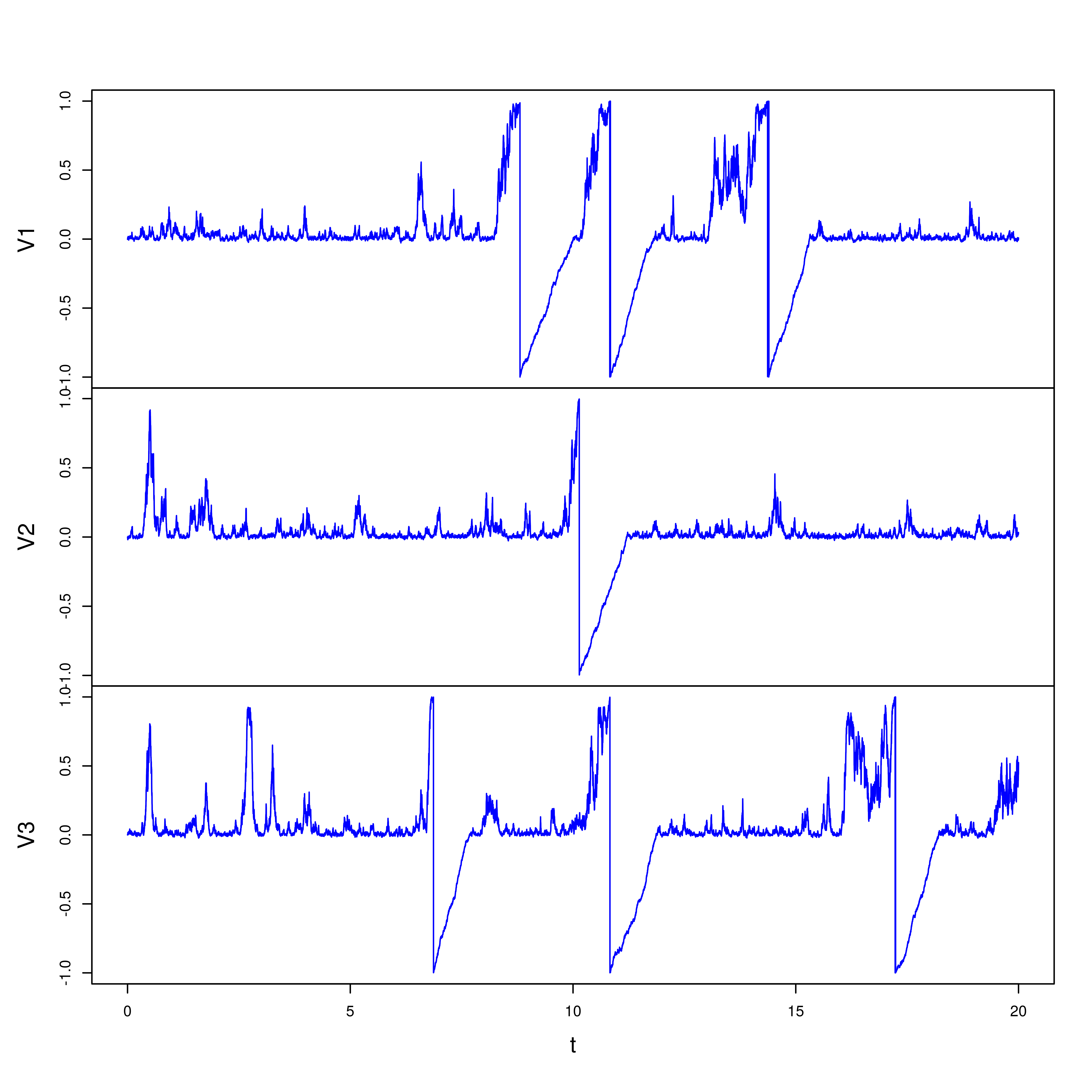
A possible more accurate model of the inhibition phase could require that also the noise term be switched off during the refractory period, that is, in our setting, as VV becomes larger than 11. We are forced to include a small noise also in the inhibition phase, for mathematical reasons (i.e., we need ϵ\epsilon below to be strictly positive, see in particular Theorems 2.2 and 3.3 and Lemma 5.1). The effect of oscillations due to the noise at the transition between the active phase and the inhibition phase appears to be negligible on macroscopic scales, thanks to the drift (see for example figure 1(b)). On the other hand, the analysis of a model in which noise contributes only to the charging phase is mathematically extremely interesting, and we will face it in a future work.

Now we will introduce precisely the equations describing the model and will give an account of our results and of the following sections. We also include some figures obtained simulating our model for a finite number of interacting neurons, showing that, even if simple, the model we propose gives a realistic description of single neurons and networks.

1.1 The model

For a Borel set AA in an euclidean space, we will denote by ℒA\mathscr{L}_{A} the Lebesgue measure restricted to AA.
Let (Ω,ℱ,ℙ)(\Omega,\mathcal{F},\mathds{P}) be a probability space, let DD be an open connected domain in ℝ3\mathds{R}^{3} and [0,T]⊂ℝ[0,T]\subset\mathds{R} a time interval. The microscopic model is as follows: for each N∈ℕN\in\mathds{N}\, consider NN neurons, each identified by

  1. i.

    its position X0i=ξiX^{i}_{0}=\xi^{i}, where ξi\xi^{i}, i∈ℕi\in\mathds{N}\, are i.i.d. random variables with finite first moment and such that ∀i\forall i ℙ⁡(ξi∈D)=1\mathds{P}\left(\xi^{i}\in D\right)=1. We denote by ν\nu the law of each ξi\xi^{i}. Since the neurons do not move, their position is modeled by the system of trivial equations

    d​Xti=0,X0i=ξi​;\,\mathrm{d}X^{i}_{t}=0\ ,\quad X^{i}_{0}=\xi^{i}\ \text{;} (1)
  2. ii.

    its action potential given by Vti,N(mod2)∈[0,2)V^{i,N}_{t}\pmod{2}\in[0,2), where Vti,N∈ℝV^{i,N}_{t}\in\mathds{R} is the strong solution to

    d​Vti,N=λ⁡(Vti,N(mod2))​d​t+1N∑j=1Nθ(ξi,ξj)𝟙[1,1+δ](Vj,Nt(mod2))𝟙[0,1](Vi,Nt(mod2))dt+σϵ​(Vti,N(mod2))​d​Bti,\,\mathrm{d}V^{i,N}_{t}=\lambda\left(V^{i,N}_{t}\pmod{2}\right)\,\mathrm{d}t\\ +\frac{1}{N}\sum_{j=1}^{N}\theta\left({\xi^{i}},{\xi^{j}}\right)\mathds{1}_{[1,1+\delta]}\left(V^{j,N}_{t}\pmod{2}\right)\mathds{1}_{[0,1]}\left(V^{i,N}_{t}\pmod{2}\right)\,\mathrm{d}t\\ +\sigma^{\epsilon}\left(V^{i,N}_{t}\pmod{2}\right)\,\mathrm{d}B^{i}_{t}\ , (2)

    with initial condition V0i,N=ηi∈[0,2)V^{i,N}_{0}=\eta^{i}\in[0,2). We assume that all random variables ηi\eta^{i} are i.i.d with law ρ~0​ℒ[0,2)\tilde{\rho}_{0}\mathscr{L}_{[0,2)} and ρ~0∈L2​(0,2)\tilde{\rho}_{0}\in L^{2}(0,2). Moreover, we assume that {ξ1,…,ξN,η1,…​ηN}\{\xi^{1},...,\xi^{N},\eta^{1},...\eta^{N}\} are independent for any N∈ℕN\in\mathds{N}\,.

    The functions appearing above are given by

    λ⁡(v)=−λ^​v​𝟙[0,1]​(v)+𝟙(1,2)​(v), with ​λ^>0;\lambda(v)=-\hat{\lambda}v\mathds{1}_{[0,1]}(v)+\mathds{1}_{(1,2)}(v),\ \text{ with }\hat{\lambda}>0\ ;
    θ⁡(x,y)​ is a bounded uniformly continuous function on ​D×D;\theta(x,y)\text{ is a bounded uniformly continuous function on }D\times D\ ;
    σϵ​(v)​ is a Cb1​([0,2])-function such that ​σϵ≥2​ϵ>0\displaystyle\sigma^{\epsilon}(v)\text{ is a $C_{b}^{1}([0,2])$-function such that \;}\sigma^{\epsilon}\geq\sqrt{2\epsilon}>0\
     and ​σϵ​(v)=2​ϵ​ on ​[1,2],σϵ​(2)=σϵ​(0)=2​ϵ,\displaystyle\text{ and }\sigma^{\epsilon}(v)=\sqrt{2\epsilon}\;\text{ on }[1,2],\;\sigma^{\epsilon}(2)=\sigma^{\epsilon}(0)=\sqrt{2\epsilon},
    d​σϵd​x​(0)=d​σϵd​x​(2)=0, with ​ϵ​ fixed.\displaystyle\frac{d\sigma^{\epsilon}}{dx}(0)=\frac{d\sigma^{\epsilon}}{dx}(2)=0\ ,\text{ with }\epsilon\text{ fixed}.

    For each i∈ℕi\in\mathds{N}\, the processes (Bti)\left(B^{i}_{t}\right) are independent real-valued Brownian motions, independent of (ξi)\left(\xi^{i}\right) and (ηi)\left(\eta^{i}\right), and δ\delta is a fixed real number in (0,1)(0,1).

Refer to caption
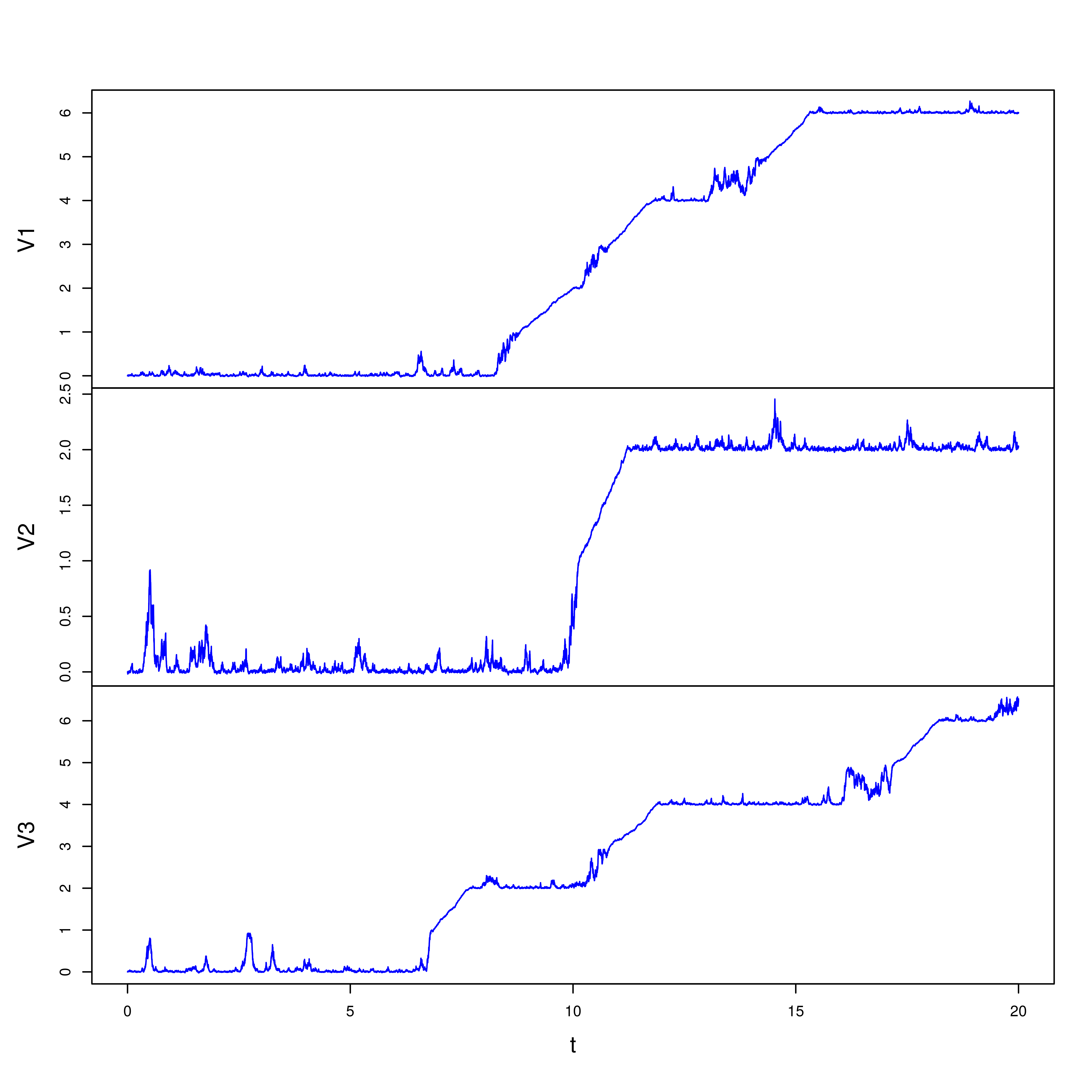
(a) Solutions Vi,3V^{i,3}, i=1,2,3i=1,2,3
Refer to caption
(b) Solutions Vi,3(mod2)V^{i,3}\pmod{2}, i=1,2,3i=1,2,3
Figure 1: Simulation of the system (2) for 33 neurons with no spatial interaction.

One could use as λ\lambda any bounded function on [0,2)[0,2) that has a jump discontinuity in v=1v=1 and is continuous elsewhere; all the results herein apply in this case with no modifications in the arguments, therefore we stick to the simple case given just above.
We will show that for each NN the system of equations (2) has a unique solution (Vi,N)i=1,…,N\left(V^{i,N}\right)_{i=1,\dots,N} with Vi,NV^{i,N} having continuous trajectories in ℝ\mathds{R}. This forces the trajectories of Vi,N(mod2)V^{i,N}\pmod{2} to have jump discontinuities at every tt such that Vti,N∈2​ℤV^{i,N}_{t}\in 2\mathds{Z}\,. However continuity is easily restored seeing Vi,N(mod2)V^{i,N}\pmod{2} as a process with values on the torus 𝕋:=ℝ/2​ℤ\mathds{T}\,:=\mathds{R}/2\mathds{Z}\, (where 2​ℤ2\mathds{Z}\, is seen as a subgroup of translations on ℝ\mathds{R}). This corresponds to considering the interval [0,2][0,2] with the identification 0≡20\equiv 2. Moreover 𝕋\mathds{T}\, is homeomorphic to 1/π​S1⊂ℝ2\nicefrac{{1}}{{\pi}}S^{1}\subset\mathds{R}^{2}, the circle with radius 1/π\nicefrac{{1}}{{\pi}}.

On 𝕋\mathds{T}\, we consider the metric

d𝕋​(v1,v2)=min⁡{(v1−v2)(mod2),(v2−v1)(mod2)}d_{\mathds{T}}\,(v_{1},v_{2})=\min\left\{(v_{1}-v_{2})\pmod{2},(v_{2}-v_{1})\pmod{2}\right\} (3)

where on the right-had side v1v_{1} and v2v_{2} are seen as elements in [0,2)⊂ℝ[0,2)\subset\mathds{R}; this corresponds to the shortest-path (or geodesic) metric, which is the arc-length on S1S^{1}. This metric induces the quotient topology on 𝕋\mathds{T}\,.
We will always consider the Euclidean metric on DD and endow D×𝕋D\times\mathds{T}\, with the product metric, denoted by dD×𝕋d_{D\times\mathds{T}\,}.
The choice to represent solutions on the torus is natural since the coefficients we introduced above are clearly 22-periodic. To stress periodicity and also to lighten notation for v∈ℝv\in\mathds{R} and x,y∈Dx,y\in D we define the functions

λ2​(v):=λ⁡(v(mod2)),\displaystyle\lambda_{2}(v):=\lambda\big(v\pmod{2}\big)\ ,
g2​(x,v,y,w):=θ⁡(x,y)​𝟙[1,1+δ]​(w(mod2))​𝟙[0,1]​(v(mod2)),\displaystyle g_{2}(x,v,y,w):=\theta(x,y)\mathds{1}_{[1,1+\delta]}\big(w\pmod{2}\big)\mathds{1}_{[0,1]}\big(v\pmod{2}\big)\ ,
σ2ϵ​(v):=σϵ​(v(mod2))\displaystyle\sigma^{\epsilon}_{2}(v):=\sigma^{\epsilon}\big(v\pmod{2}\big)\

so that equation (2) takes the more readable form

d​Vti,N=λ2​(Vti,N)​d​t+1N​∑j=1Ng2​(ξi,Vti,N,ξj,Vtj,N)​d​t+σ2ϵ​(Vti,N)​d​Bti.\,\mathrm{d}V^{i,N}_{t}=\lambda_{2}\left(V^{i,N}_{t}\right)\,\mathrm{d}t+\frac{1}{N}\sum_{j=1}^{N}g_{2}\left({\xi^{i}},V^{i,N}_{t},{\xi^{j}},V^{j,N}_{t}\right)\,\mathrm{d}t+\sigma^{\epsilon}_{2}\left(V^{i,N}_{t}\right)\,\mathrm{d}B^{i}_{t}\ . (4)

Since 𝕋\mathds{T}\, is homeomorphic to 1/π​S1⊂ℝ2\nicefrac{{1}}{{\pi}}S^{1}\subset\mathds{R}^{2}, one can define the Lebesgue measure on 𝕋\mathds{T}\, as the push-forward of the Lebesgue measure on [0,2)[0,2) through the map t↦(cos⁡(π​t),sin⁡(π​t))t\mapsto(\cos(\pi t),\sin(\pi t)); since 𝕋\mathds{T}\, is endowed with the quotient topology, any measure on the Borel sets of 𝕋\mathds{T}\, can be obtained in this way. Therefore we can interpret a Borel measure on D×𝕋D\times\mathds{T}\, as a Borel measure on D×[0,2)D\times[0,2), and we will do so henceforth. Notice that any Borel measure on 𝕋\mathds{T}\, defines a Borel measure on the whole ℝ\mathds{R} by 22-periodic replication; we will not distinguish between the two in the sequel.
We will show that the solution to (4) has a density which is 22-periodic, thanks to the form of the coefficients; hence this density can be identified with a Borel measure on D×𝕋D\times\mathds{T}\,.

Refer to caption
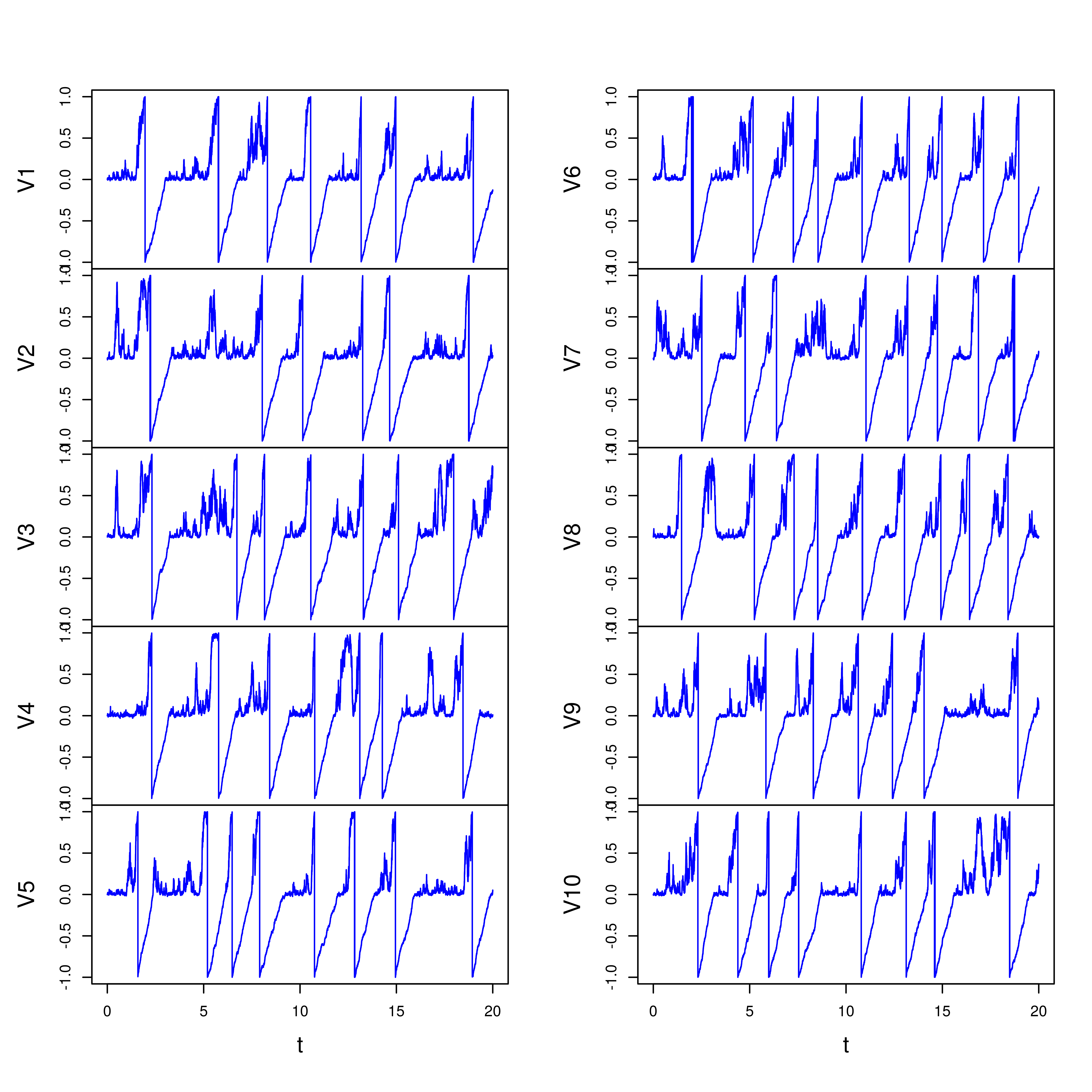
(a) Solutions Vi,10V^{i,10}
Refer to caption
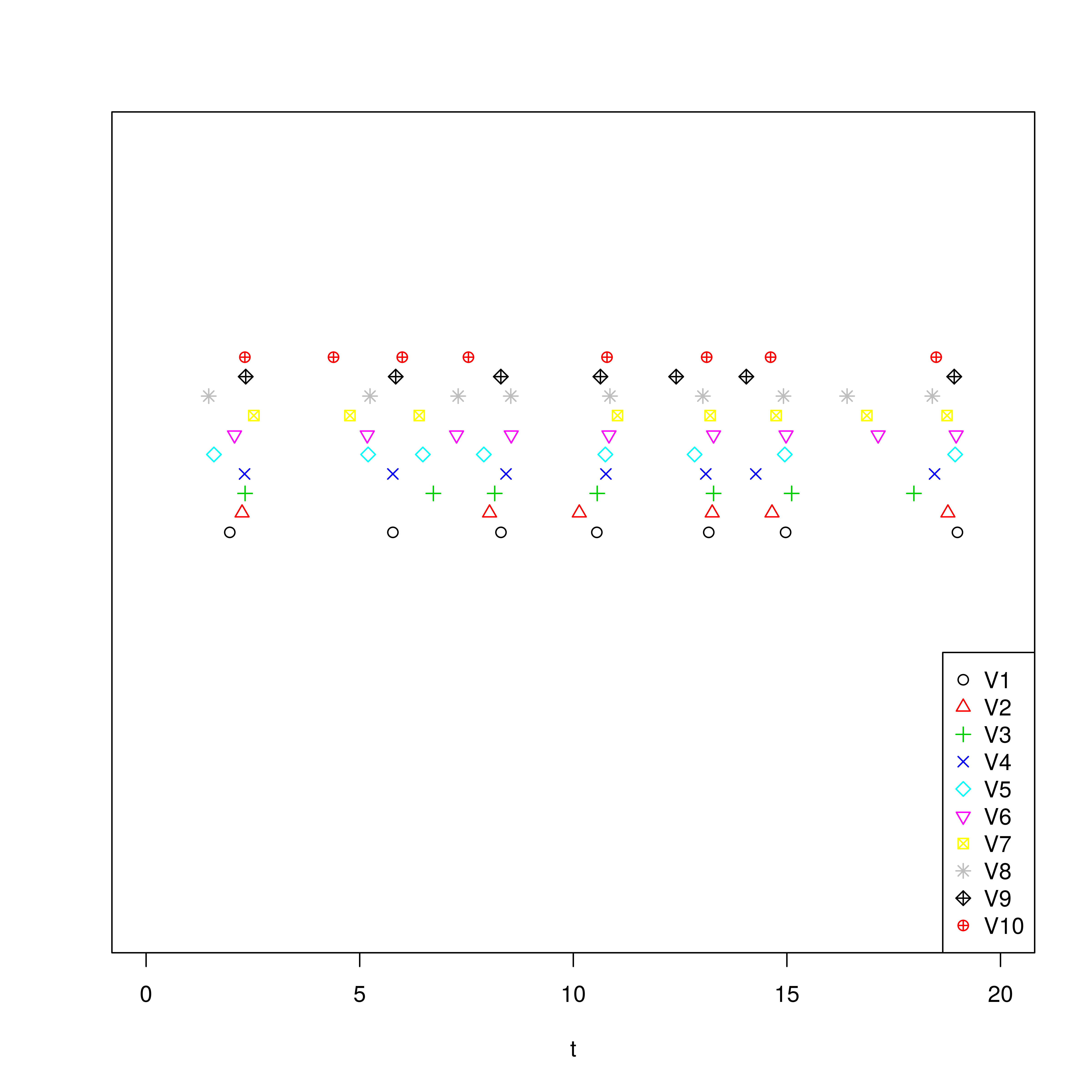
(b) Spikes of each neuron in time
Figure 2: Solution of system (2) for 1010 neurons with strong interaction uniform in space. A spike from one neuron propagates to all other neurons in the network

Let StNS_{t}^{N} denote the empirical measure

StN=1N​∑i=1Nδ(ξi,Vti,N​(mod​2))=1N​∑i=1Nδ(ξi,Vti,N​(mod​2))S_{t}^{N}=\frac{1}{N}\sum_{i=1}^{N}\delta_{\left({\xi^{i}},V_{t}^{i,N}\mkern 4.0mu({\operator@font mod}\mkern 6.0mu2)\right)}=\frac{1}{N}\sum_{i=1}^{N}\delta_{\left(\xi^{i},V^{i,N}_{t}\mkern 4.0mu({\operator@font mod}\mkern 6.0mu2)\right)}\ (5)

and set for every x,y∈Dx,y\in D and v∈ℝv\in\mathds{R}

σ2ϵ(x,v):=σ2ϵ(v),θ(x,y,v):=θ(x,y) and λ2(x,v):=λ2(v)\sigma^{\epsilon}_{2}(x,v):=\sigma^{\epsilon}_{2}(v)\ ,\quad\theta(x,y,v):=\theta(x,y)\quad\text{ and }\quad\lambda_{2}(x,v):=\lambda_{2}(v)

for later use (see for instance (8)). To any function ϕ\phi on D×𝕋D\times\mathds{T}\, which is continuous corresponds a unique continuous function on D×ℝD\times\mathds{R} that is 22-periodic with respect to its second variable, given by (x,v)↦ϕ⁡(x,v⁡(mod​2))(x,v)\mapsto\phi(x,v\mkern 4.0mu({\operator@font mod}\mkern 6.0mu2)); in the sequel we will identify these two functions and denote by ϕ\phi also its 22-periodic representation on D×ℝD\times\mathds{R}. With this convention, for any smooth and compactly supported function ϕ\phi on D×𝕋D\times\mathds{T}\, we have

d⁡⟨StN,ϕ⟩=d​1N​∑i=1Nϕ⁡(X0i,Vti,N)=1N​∑i=1N∂vϕ⁡(X0i,Vti,N)​(λ2​(Vti,N)+1N​∑j=1Ng2​(X0i,Vti,N,X0j,Vtj,N))​d​t+1N∑i=1Nσϵ2(Vi,Nt)∂vϕ(X0i,Vi,Nt)dBit+1N∑i=1Nσ2ϵ​(Vti,N)22∂2vϕ(X0i,Vi,Nt)dt=⟨SNt,λ2∂vϕ⟩dt+⟨SNt,⟨SNt,g2(x,v,⋅,⋅)⟩∂vϕ⟩dt+⟨SNt,(σ2ϵ)22∂2vϕ⟩dt+dMtN,ϕ\,\mathrm{d}\langle S^{N}_{t},\phi\rangle=\,\mathrm{d}\frac{1}{N}\sum_{i=1}^{N}\phi\left(X_{0}^{i},V_{t}^{i,N}\right)\\ =\frac{1}{N}\sum_{i=1}^{N}\partial_{v}\phi\left(X_{0}^{i},V^{i,N}_{t}\right)\left(\lambda_{2}\left(V^{i,N}_{t}\right)+\frac{1}{N}\sum_{j=1}^{N}g_{2}\left(X_{0}^{i},V^{i,N}_{t},X_{0}^{j},V^{j,N}_{t}\right)\right)\,\mathrm{d}t\\ +\frac{1}{N}\sum_{i=1}^{N}\sigma^{\epsilon}_{2}\left(V^{i,N}_{t}\right)\partial_{v}\phi\left(X_{0}^{i},V^{i,N}_{t}\right)\,\mathrm{d}B^{i}_{t}+\frac{1}{N}\sum_{i=1}^{N}\frac{\sigma^{\epsilon}_{2}\left(V^{i,N}_{t}\right)^{2}}{2}\partial^{2}_{v}\phi\left(X_{0}^{i},V^{i,N}_{t}\right)\,\mathrm{d}t\\[8.53581pt] =\langle S^{N}_{t},\lambda_{2}\partial_{v}\phi\rangle\,\mathrm{d}t+\langle S^{N}_{t},\langle S^{N}_{t},g_{2}(x,v,\cdot,\cdot)\rangle\partial_{v}\phi\rangle\,\mathrm{d}t+\langle S^{N}_{t},\frac{\left(\sigma_{2}^{\epsilon}\right)^{2}}{2}\partial^{2}_{v}\phi\rangle\,\mathrm{d}t+\,\mathrm{d}M_{t}^{N,\phi}\ (6)

where we use the notation

⟨StN,⟨StN,g2(x,v,⋅,⋅)⟩∂vϕ⟩=∫D×𝕋∂vϕ(x,v)StN(dx,dv)∫D×𝕋g2(x,v,y,w)StN(dy,dw)\langle S^{N}_{t},\langle S^{N}_{t},g_{2}(x,v,\cdot,\cdot)\rangle\partial_{v}\phi\rangle=\int_{D\times\mathds{T}\,}\partial_{v}\phi(x,v)S^{N}_{t}(\,\mathrm{d}x,\,\mathrm{d}v)\int_{D\times\mathds{T}\,}g_{2}(x,v,y,w)S^{N}_{t}(\,\mathrm{d}y,\,\mathrm{d}w) (7)

and

MtN,ϕ=∫0t1N​∑i=1Nσ2ϵ​(Vsi,N)​∂vϕ⁡(Xi,Vsi,N)​d​BsiM^{N,\phi}_{t}=\int_{0}^{t}\frac{1}{N}\sum_{i=1}^{N}\sigma^{\epsilon}_{2}\left(V^{i,N}_{s}\right)\partial_{v}\phi\left(X^{i},V^{i,N}_{s}\right)\,\mathrm{d}B^{i}_{s}

is a martingale such that 𝔼⁡[supt|MtN,ϕ|2]→0\mathds{E}\big[\sup_{t}\left|M^{N,\phi}_{t}\right|^{2}\big]\to 0 as N→∞N\to\infty (due to the stochastic integrals being uncorrelated).
If we suppose that the sequence of random measures StN​(d​x,d​v)S^{N}_{t}(\,\mathrm{d}x,\,\mathrm{d}v) converges in probability (in a suitable space) to a probability measure ρt​(x,v)​d​x​d​v\rho_{t}(x,v)\,\mathrm{d}x\,\mathrm{d}v on D×𝕋D\times\mathds{T}\,, then, heuristically, a passage to the limit in NN suggests that ρt\rho_{t} solves weakly the partial differential equation of Fokker-Planck type

∂∂t​ρt​(x,v)=12​∂2∂v2​((σ2ϵ)2​ρt)​(x,v)−∂∂v​(λ2​ρt)​(x,v)−∂∂v​(ρt​∫g2​(⋅,⋅,y,w)​ρt​(y,w)​dy​dw)​(x,v).\frac{\partial}{\partial t}\rho_{t}(x,v)=\frac{1}{2}\frac{\partial^{2}}{\partial v^{2}}\left(\left(\sigma_{2}^{\epsilon}\right)^{2}\rho_{t}\right)(x,v)-\frac{\partial}{\partial v}\left(\lambda_{2}\rho_{t}\right)(x,v)\\ -\frac{\partial}{\partial v}\left(\rho_{t}\int g_{2}(\cdot,\cdot,y,w)\rho_{t}(y,w)\,\mathrm{d}y\,\mathrm{d}w\right)(x,v)\ . (8)

In the sequel we will prove rigorously a similar assertion involving measures μt\mu_{t} instead of densities ρt\rho_{t}.

Refer to caption
Refer to caption
Refer to caption
Figure 3: A network made of two subnetworks with localized strong interaction. Each blue line corresponds to the presence of interaction; only one neuron of the first subnetwork interacts with a single neuron of the second one. The vertical axis represents time; the network is drawn on the t=0t=0 plane and to each spike of a neuron corresponds a sphere above it, with the same color as the neuron. Near time t=1t=1 many neurons in the first network spike and the signal is propagated to the second network, while at time t=2t=2 the signal does not propagate to the second network.

1.2 Main results

The main aim of the paper is to show that the empirical measure actually converges in a weak sense to a limiting probability measure μt​(d​x,d​v)\mu_{t}(\,\mathrm{d}x,\,\mathrm{d}v) such that the marginal with respect to vv has a L2L^{2}-density and which is the unique solution to the above PDE (8). This is the content of Theorem 5.7.
The paper is organized as follows. In Section 2 we will prove strong well-posedness for the system of SDEs (2); a modification of the standard theory for finite-dimensional SDEs with bounded and measurable drift is needed here to deal with the dependence of the equations on the random variables X0iX_{0}^{i}. In Section 3 we define a weak measure-valued solution and show that the PDE (8) has at most one such solution.
To show existence of a solution to the PDE we first prove that the laws ℚN\mathds{Q}\,^{N} of the empirical measures of (Xi,Vi,N​(mod​2))(X^{i},V^{i,N}\mkern 4.0mu({\operator@font mod}\mkern 6.0mu2)) (see (5)) are tight as probability measures on the space of continuous measure-valued functions of time (Section 4). Then we prove that any limit point ℚ\mathds{Q}\, of ℚN\mathds{Q}\,^{N} gives full measure to the set of functions with values that are continuous measures with marginal with respect to vv having a L2L^{2}-density, that ℚ\mathds{Q}\, is supported by the set of weak measure-valued solutions to the Fokker-Planck PDE and that actually all the sequence ℚN\mathds{Q}\,^{N} converges to the same limit. This provides existence of a solution and is discussed in Section 5.
Section 6 briefly shows that well-posedness of the Fokker-Planck PDE implies existence of a unique strong solution to the McKean-Vlasov SDE associated with the particle system. We conclude with an appendix giving some immediate generalizations of our results together with some indications on how the proofs have to be adapted to this more general setting.

2 The system of particles

Consider independent Brownian motions BiB^{i}, i∈ℕi\in\mathds{N}\, and assume that the random variables ηi\eta^{i} introduced in the previous section are i.i.d. and independent from all BiB^{i}; denote by (ℱt0)t(\mathcal{F}^{0}_{t})_{t} the filtration ℱt0=σ(Bsi,0≤s≤t,i∈ℕ)∨σ(ηi,i∈ℕ)\mathcal{F}^{0}_{t}=\sigma\left(B^{i}_{s},0\leq s\leq t,i\in\mathds{N}\,\right)\vee\sigma(\eta^{i},i\in\mathds{N}\,) augmented with the ℙ\mathds{P}-null sets.
We also denote by 𝒢{\cal G} the σ\sigma-algebra σ⁡(ξi,i∈ℕ)\sigma\left(\xi^{i},i\in\mathds{N}\,\right) and assume that for any t≥0t\geq 0, 𝒢{\mathcal{G}} and ℱt0{\mathcal{F}}_{t}^{0} are independent.
Finally we introduce the filtration (ℱt)(\mathcal{F}_{t}) where ℱt\mathcal{F}_{t} is the completion of ℱt0∨𝒢\mathcal{F}_{t}^{0}\vee\mathcal{G}.

Let us write our system of equations in vector form: we fix N∈ℕN\in\mathds{N}\, and introduce, for the variables 𝐯=(v1,…,vN)⊤∈ℝN\mathbf{v}=(v^{1},\dots,v^{N})^{\top}\in\mathds{R}^{N}, 𝐱=(x1,…,xN)⊤∈DN\mathbf{x}=(x^{1},\dots,x^{N})^{\top}\in D^{N}, the functions

λ¯2:ℝN→ℝN\displaystyle\bar{\lambda}_{2}:\mathds{R}^{N}\to\mathds{R}^{N}
λ¯2​(𝐯)=(λ2​(v1),…,λ2​(vN))⊤,\displaystyle\bar{\lambda}_{2}(\mathbf{v})=\left(\lambda_{2}(v^{1}),\dots,\lambda_{2}(v^{N})\right)^{\top}\ ,
g¯2:(D×ℝ)N+1→ℝN\displaystyle\bar{g}_{2}:\left(D\times\mathds{R}\right)^{N+1}\to\mathds{R}^{N}
g¯2​(𝐱,𝐯,y,w)=(g2​(x1,v1,y,w),…,g2​(xN,vN,y,w))⊤,\displaystyle\bar{g}_{2}(\mathbf{x},\mathbf{v},y,w)=\left(g_{2}(x^{1},v^{1},y,w),\dots,g_{2}(x^{N},v^{N},y,w)\right)^{\top},
σ¯2ϵ:ℝN→ℝN×N\displaystyle\bar{\sigma}_{2}^{\epsilon}:\mathds{R}^{N}\to\mathds{R}^{N\times N}
σ¯2ϵ​(𝐯)=diag⁡(σ2ϵ​(v1),…,σ2ϵ​(vN)).\displaystyle\bar{\sigma}_{2}^{\epsilon}(\mathbf{v})=\diag\left(\sigma_{2}^{\epsilon}(v^{1}),\dots,\sigma_{2}^{\epsilon}(v^{N})\right).

Setting Ξ=(ξ1,…,ξN)\Xi=\left(\xi^{1},\dots,\xi^{N}\right), Ψ=(η1,…,ηN)\Psi=\left(\eta^{1},\dots,\eta^{N}\right), we want to show existence and uniqueness of strong solutions to

{d​𝐕t=λ¯2​(𝐕t)​d​t+1N​∑j=1Ng¯2​(Ξ,𝐕t,Ξj,Vtj)​d​t+σ¯2ϵ​(𝐕t)​d​𝐁t𝐕0=Ψ.\begin{cases}\,\mathrm{d}\mathbf{V}_{t}=\bar{\lambda}_{2}\left(\mathbf{V}_{t}\right)\,\mathrm{d}t+\frac{1}{N}\sum_{j=1}^{N}\bar{g}_{2}\left(\Xi,\mathbf{V}_{t},\Xi^{j},V^{j}_{t}\right)\,\mathrm{d}t+\bar{\sigma}^{\epsilon}_{2}\left(\mathbf{V}_{t}\right)\,\mathrm{d}\mathbf{B}_{t}\\ \mathbf{V}_{0}=\Psi\ .\end{cases} (9)

The classical reference for existence of a strong solution for SDEs with bounded measurable drift is [Ver81]. However, the results proved therein do not apply directly to equation (9), because they do not guarantee the measurable dependence of the solution VV on the stochastic parameter Ξ\Xi. Therefore we introduce the following definition.

Let us denote by 𝒮\mathcal{S} the Banach space of all continuous paths from [0,T][0,T] into ℝN\mathds{R}^{N} endowed with the supremum norm |⋅|𝒮\lvert\cdot\rvert_{\mathcal{S}}. We also denote by νN\nu_{N} the law of the random variable Ξ\Xi on the Borel σ\sigma-algebra of DND^{N}.

Definition 2.1 (Strong solution).

A strong solution to (9) is a family of continuous ℝN\mathds{R}^{N}-valued ℱt0{\cal F}_{t}^{0}-adapted processes (𝐕t𝐱)({\bf V}^{{\bf x}}_{t}), 𝐱∈DN{\bf x}\in D^{N}, such that

  1. ((i))

    the mapping (𝐱,ω)↦𝐕⋅𝐱​(ω)∈𝒮({\bf x},\omega)\mapsto{\bf V}_{\cdot}^{{\bf x}}(\omega)\in\mathcal{S} is measurable from (DN×Ω,ℬ⁡(DN)×ℱ)(D^{N}\times\Omega,{\cal B}(D^{N})\times{\cal F}) to (𝒮,ℬ⁡(𝒮))(\mathcal{S},{\cal B}(\mathcal{S}));

  2. ((ii))

    for νN\nu_{N}-almost every 𝐱∈DN{\bf x}\in D^{N}, (𝐕t𝐱)({\bf V}_{t}^{{\bf x}}) satisfies equation (9) in the strong sense when Ξ=𝐱\Xi={\bf x}.

The above definition is motivated by the fact that if (𝐕t𝐱)({\bf V}^{{\bf x}}_{t}) is a strong solution, then the ℱt{\cal F}_{t}-adapted process (𝐕𝐭𝚵)({\bf V_{t}^{\Xi}}) satisfies equation (9) ℙ\mathds{P}-almost surely for any t∈[0,T]t\in[0,T]. In fact, for Ξ\Xi random variable as above, the process (𝐕tΞ)({\bf V}^{\Xi}_{t}) is well-defined with values in ℝN\mathds{R}^{N}, has continuous paths and is ℱt{\mathcal{F}}_{t}-adapted.
To prove that (𝐕tΞ)\left(\mathbf{V}^{\Xi}_{t}\right) satisfies (9) it is enough to compute, using conditional expectation with respect to 𝒢\cal G and independence,

𝔼​|Ψ+∫0tλ¯2​(𝐕rΞ)​𝑑r+1N​∑j=1N∫0tg¯2​(Ξ,𝐕rΞ,Ξj,VrΞ,j)​𝑑r+∫0tσ¯2ϵ​(𝐕rΞ)​d​𝐁r−𝐕tΞ|\displaystyle\mathds{E}\left|\Psi+\int_{0}^{t}\bar{\lambda}_{2}\left(\mathbf{V}^{\Xi}_{r}\right)\,\mathrm{d}r+\frac{1}{N}\sum_{j=1}^{N}\int_{0}^{t}\bar{g}_{2}\left(\Xi,\mathbf{V}^{\Xi}_{r},\Xi^{j},{V}^{\Xi,j}_{r}\right)\,\mathrm{d}r+\int_{0}^{t}\bar{\sigma}^{\epsilon}_{2}\left(\mathbf{V}^{\Xi}_{r}\right)\,\mathrm{d}\mathbf{B}_{r}-{\bf V}_{t}^{\Xi}\right|
=𝔼​𝔼​[|Ψ+∫0tλ¯2​(𝐕rΞ)​𝑑r+1N​∑j=1N∫0tg¯2​(Ξ,𝐕rΞ,Ξj,VrΞ,j)​𝑑r+∫0tσ¯2ϵ​(𝐕rΞ)​d​𝐁r−𝐕tΞ|​𝒢]\displaystyle=\mathds{E}\mathds{E}\left[\left|\Psi+\int_{0}^{t}\bar{\lambda}_{2}\left(\mathbf{V}^{\Xi}_{r}\right)\,\mathrm{d}r+\frac{1}{N}\sum_{j=1}^{N}\int_{0}^{t}\bar{g}_{2}\left(\Xi,\mathbf{V}^{\Xi}_{r},\Xi^{j},V^{\Xi,j}_{r}\right)\,\mathrm{d}r+\int_{0}^{t}\bar{\sigma}^{\epsilon}_{2}\left(\mathbf{V}^{\Xi}_{r}\right)\,\mathrm{d}\mathbf{B}_{r}-{\bf V}_{t}^{\Xi}\right|\ {\cal G}\right]
=𝔼​𝔼​[|Ψ+∫0tλ¯2​(𝐕r𝐱)​𝑑r+1N​∑j=1N∫0tg¯2​(𝐱,𝐕r𝐱,xj,Vr𝐱,j)​𝑑r+∫0tσ¯2ϵ​(𝐕r𝐱)​d​𝐁r−𝐕t𝐱|𝐱=Ξ]\displaystyle=\mathds{E}\mathds{E}\left[\left|\Psi+\int_{0}^{t}\bar{\lambda}_{2}\left(\mathbf{V}^{\mathbf{x}}_{r}\right)\,\mathrm{d}r+\frac{1}{N}\sum_{j=1}^{N}\int_{0}^{t}\bar{g}_{2}\left(\mathbf{x},\mathbf{V}^{\mathbf{x}}_{r},x^{j},{V}^{{\mathbf{x}},j}_{r}\right)\,\mathrm{d}r+\int_{0}^{t}\bar{\sigma}^{\epsilon}_{2}\left(\mathbf{V}^{\mathbf{x}}_{r}\right)\,\mathrm{d}\mathbf{B}_{r}-{\bf V}_{t}^{\mathbf{x}}\right|_{{\bf x}=\Xi}\right]
=0.\displaystyle=0.
Theorem 2.2.

For every N∈ℕN\in\mathds{N}\, there exists a strong solution to (4). Two strong solutions on the same probability space associated to the same initial condition Ψ\Psi are indistinguishable for νN\nu_{N}-almost every 𝐱∈DN{\bf x}\in D^{N}.

Proof.

Existence. First fix 𝐱∈DN{\bf x}\in D^{N}; the SDE

{d​𝐕t𝐱=λ¯2​(𝐕t𝐱)​d​t+1N​∑j=1Ng¯2​(𝐱,𝐕t𝐱,xj,Vt𝐱,j)​d​t+σ¯2ϵ​(𝐕t𝐱)​d​𝐁t𝐕0𝐱=Ψ.\begin{cases}\,\mathrm{d}\mathbf{V}^{\mathbf{x}}_{t}=\bar{\lambda}_{2}\left(\mathbf{V}^{\mathbf{x}}_{t}\right)\,\mathrm{d}t+\frac{1}{N}\sum_{j=1}^{N}\bar{g}_{2}\left(\mathbf{x},\mathbf{V}^{\mathbf{x}}_{t},x^{j},V^{{\mathbf{x}},j}_{t}\right)\,\mathrm{d}t+\bar{\sigma}^{\epsilon}_{2}\left(\mathbf{V}^{\mathbf{x}}_{t}\right)\,\mathrm{d}\mathbf{B}_{t}\\ \mathbf{V}^{\mathbf{x}}_{0}=\Psi\ .\end{cases} (10)

admits a unique strong solution 𝐕𝐱\mathbf{V}^{\mathbf{x}} by the results proved in [Ver81]. We now clarify the measurability of 𝐕𝐱{\bf V^{x}} with respect to 𝐱{\bf x}. One difficulty is that the proof of the main well-posedness results in [Ver81] is based on the Yamada-Watanabe theorem and is indeed abstract and non-contructive. This is why to prove such a measurability property we follow the approach in [GK96]. Fix a sequence of partitions {πn}n∈ℕ\left\{\pi^{n}\right\}_{n\in\mathds{N}\,} of [0,T][0,T], where each πn\pi^{n} is given by points 0=t0n<t1n<⋯<tnn=T0=t_{0}^{n}<t_{1}^{n}<\dots<t_{n}^{n}=T, set κn​(t)=∑i=0n−1tin​𝟙[tin,ti+1n)​(t)\kappa^{n}(t)=\sum_{i=0}^{n-1}t_{i}^{n}\mathds{1}_{[t_{i}^{n},t_{i+1}^{n})}(t) and consider Euler’s approximations to equation (10) given by

{d​𝐕t𝐱,n=λ¯2​(𝐕𝐱,n​(κn​(t)))​d​t+1N​∑j=1Ng¯2​(𝐱,𝐕𝐱,n​(κn​(t)),xj,V𝐱,n,j​(κn​(t)))​d​t+σ¯2ϵ​(𝐕𝐱,n​(κn​(t)))​d​𝐁t,𝐕0𝐱,n=Ψ.\begin{cases}\,\mathrm{d}\mathbf{V}^{\mathbf{x},n}_{t}=\bar{\lambda}_{2}\left(\mathbf{V}^{\mathbf{x},n}(\kappa^{n}(t))\right)\,\mathrm{d}t+\frac{1}{N}\sum_{j=1}^{N}\bar{g}_{2}\left(\mathbf{x},\mathbf{V}^{\mathbf{x},n}(\kappa^{n}(t)),x^{j},V^{{\mathbf{x}},n,j}(\kappa^{n}(t))\right)\,\mathrm{d}t\\ \phantom{aaaaaaaaaaaaaaaaaaaaaaaaaaaaaaaaaaaaaaaaaaaaaa}+\bar{\sigma}^{\epsilon}_{2}\left(\mathbf{V}^{\mathbf{x},n}(\kappa^{n}(t))\right)\,\mathrm{d}\mathbf{B}_{t},\\ \mathbf{V}^{\mathbf{x},n}_{0}=\Psi\ .\end{cases} (11)

In the next steps, we will use that, for any n≥1n\geq 1, the processes 𝐕𝐱,𝐧{\bf V^{x,n}} enjoy all the measurability properties we need.
By Theorem 2.8 in [GK96] we know that, for any 𝐱∈DN{\bf x}\in D^{N} and δ>0\delta>0

ℙ⁡(|𝐕𝐱,n−𝐕𝐱|𝒮>δ)→0,as ​n→∞.\mathds{P}\left(\left|{\bf V}^{{\bf x},n}-{\bf V}^{\bf x}\right|_{\mathcal{S}}>\delta\right)\to 0,\;\;\text{as }n\to\infty. (12)

Note that, for any p≥2p\geq 2 (using the boundedness of the coefficients of the SDEs) there exists Cp>0C_{p}>0 (independent of nn and 𝐱∈𝐃\bf{x}\in D) such that, for any n≥1n\geq 1, 𝔼⁡[|𝐕𝐱,n−𝐕𝐱|𝒮p]\mathds{E}\left[\left|{\bf V}^{{\bf x},n}-{\bf V}^{\bf x}\right|^{p}_{\mathcal{S}}\right] ≤Cp\leq C_{p}. Writing

𝔼​|𝐕𝐱,n−𝐕𝐱|𝒮2=𝔼[|𝐕𝐱,n−𝐕𝐱|2𝒮 1{|𝐕𝐱,n−𝐕𝐱|𝒮>δ}]+𝔼[|𝐕𝐱,n−𝐕𝐱|2𝒮 1{|𝐕𝐱,n−𝐕𝐱|𝒮≤δ}]\mathds{E}\left|{\bf V}^{{\bf x},n}-{\bf V}^{\bf x}\right|^{2}_{\mathcal{S}}\\ =\mathds{E}\left[\left|{\bf V}^{{\bf x},n}-{\bf V}^{\bf x}\right|^{2}_{\mathcal{S}}\,\mathds{1}_{\{|{\bf V}^{{\bf x},n}-{\bf V}^{\bf x}|_{\mathcal{S}}>\delta\}}\right]+\mathds{E}\left[\left|{\bf V}^{{\bf x},n}-{\bf V}^{\bf x}\right|^{2}_{\mathcal{S}}\,\mathds{1}_{\{|{\bf V}^{{\bf x},n}-{\bf V}^{\bf x}|_{\mathcal{S}}\leq\delta\}}\right]

and using also the Hölder inequality, we easily deduce that, for any 𝐱∈DN{\bf x}\in D^{N},

𝔼⁡[|𝐕𝐱,n−𝐕𝐱|𝒮2]→0,as ​n→∞.\mathds{E}\left[\left|{\bf V}^{{\bf x},n}-{\bf V}^{\bf x}\right|_{\mathcal{S}}^{2}\right]\to 0,\;\;\text{as }n\to\infty\ . (13)

Hence, for any 𝐱∈DN{\bf x}\in D^{N}, 𝐕𝐱,n{\bf V}^{{\bf x},n} converges to 𝐕𝐱{\bf V^{x}} in the Banach space L2​(Ω,𝒮)L^{2}(\Omega;\mathcal{S}) and so the mapping 𝐱↦𝐕𝐱∈L2​(Ω,𝒮){\bf x}\mapsto{\bf V}^{{\bf x}}\in L^{2}(\Omega;\mathcal{S}) is Borel measurable on (DN,ℬ⁡(DN))\left(D^{N},\mathcal{B}(D^{N})\right). By the dominated convergence theorem we infer

∫DN𝔼⁡[|𝐕𝐱,n−𝐕𝐱|𝒮2]​νN​(𝑑x)→0,as ​n→∞,\int_{D^{N}}\mathds{E}\left[\left|{\bf V}^{{\bf x},n}-{\bf V}^{\bf x}\right|_{\mathcal{S}}^{2}\right]\nu_{N}(\,\mathrm{d}x)\to 0,\;\;\text{as }n\to\infty\ , (14)

i.e., (𝐕⋅,n)({\bf V}^{{\bf\cdot},n}) converges to 𝐕⋅{\bf V^{\cdot}} in 𝒵=L2​((DN,νN),L2​(Ω,𝒮))\mathcal{Z}=L^{2}\left((D^{N},\nu_{N});L^{2}(\Omega;\mathcal{S})\right). It follows that (𝐕𝐱,n)({\bf V}^{{\bf x},n}) is a Cauchy sequence in 𝒵\mathcal{Z}. Using that, for any n,m≥1,n,m\geq 1,

∫DN𝔼⁡[|𝐕𝐱,n−𝐕𝐱,m|𝒮2]​νN​(𝑑x)=∫DN×Ω|𝐕𝐱,n​(ω)−𝐕𝐱,m​(ω)|𝒮2​νN​(𝑑x)​ℙ​(𝑑ω),\int_{D^{N}}\mathds{E}\left[\left|{\bf V}^{{\bf x},n}-{\bf V}^{{\bf x},m}\right|_{\mathcal{S}}^{2}\right]\nu_{N}(\,\mathrm{d}x)=\int_{D^{N}\times\Omega}\left|{\bf V}^{{\bf x},n}(\omega)-{\bf V}^{{\bf x},m}(\omega)\right|_{\mathcal{S}}^{2}\nu_{N}(\,\mathrm{d}x)\mathds{P}(\,\mathrm{d}\omega)\ , (15)

we get that (𝐕⋅,n)({\bf V}^{{\bf\cdot},n}) converges to some 𝐕~⋅{\bf\tilde{V}^{\cdot}} in L2​((DN×Ω,νN×ℙ),𝒮)L^{2}\left((D^{N}\times\Omega,\nu_{N}\times\mathds{P});\mathcal{S}\right). In particular, 𝐕~⋅{\bf\tilde{V}^{\cdot}} is measurable on (DN×Ω,ℬ⁡(DN)×ℱ)(D^{N}\times\Omega,{\mathcal{B}}(D^{N})\times{\mathcal{F}}) with values in 𝒮\mathcal{S}.
It follows that, for a.e. 𝐱∈DN{\bf x}\in D^{N}, we have 𝐕~𝐱=𝐕𝐱{\bf\tilde{V}^{x}}={\bf V^{x}} in 𝒮\mathcal{S}, ℙ\mathds{P}-a.s. (we have obtained a version of the strong solution which has the required measurability properties with respect to 𝐱{\bf x}).

Uniqueness. It follows directly from the celebrated Veretennikov result. ∎

Remark 2.3.

To show existence and uniqueness of a solution one could weaken the assumptions on the regularity of σϵ\sigma^{\epsilon}, similarly to what is done in the references [Ver81] and [GK96]. What is needed above is that pathwise uniqueness holds for equation (10), and there are many well-known conditions assuring that this happens. However at a later stage in the paper (Section 5) we will need to assume that σϵ\sigma^{\epsilon} is differentiable with bounded derivative. This does not seem to be a limitation on the model, since there is no reason to assume that the diffusion coefficient be particularly rough.

3 The limit PDE: uniqueness of measure-valued solutions

Let Pr⁡(D×𝕋)\mathrm{Pr}(D\times\mathds{T}\,) be the space of Borel probability measures over D×𝕋D\times\mathds{T}\,. Let Pr1​(D×𝕋)⊂Pr⁡(D×𝕋)\mathrm{Pr}_{1}(D\times\mathds{T}\,)\subset\mathrm{Pr}(D\times\mathds{T}\,) be the space of probability measures over D×𝕋D\times\mathds{T}\, with finite first moment, endowed with the 1-Wasserstein metric 𝒲1\mathcal{W}_{1}.
Suppose as above that the empirical measures StNS^{N}_{t} converge in a weak sense to a probability measure μt\mu_{t} on D×𝕋D\times\mathds{T}\,. Without assuming that μt\mu_{t} has a density, we expect that it solve the PDE

∂∂t​μt=12​∂2∂v2​((σ2ϵ)2​μt)−∂∂v​(λ2​μt)−∂∂v​(μt​∫g2​(⋅,⋅,y,w)​μt​(𝑑y,𝑑w)),\frac{\partial}{\partial t}\mu_{t}=\frac{1}{2}\frac{\partial^{2}}{\partial v^{2}}\left(\left(\sigma_{2}^{\epsilon}\right)^{2}\mu_{t}\right)-\frac{\partial}{\partial v}\left(\lambda_{2}\mu_{t}\right)-\frac{\partial}{\partial v}\left(\mu_{t}\int g_{2}(\cdot,\cdot,y,w)\mu_{t}(\,\mathrm{d}y,\,\mathrm{d}w)\right)\ , (16)

with initial condition ν×ρ~0​ℒ𝕋\nu\times\tilde{\rho}_{0}\mathscr{L}_{\mathds{T}\,}\ , meaning that μ0​(d​x,d​v)=ν⁡(d​x)​ρ~0​(v)​ℒ𝕋​(d​v)\mu_{0}(\,\mathrm{d}x,\,\mathrm{d}v)=\nu(\,\mathrm{d}x)\tilde{\rho}_{0}(v)\mathscr{L}_{\mathds{T}}\,(\,\mathrm{d}v). Fix T>0T>0; we will denote by 𝒞\mathscr{C} the space

𝒞:=C⁡([0,T],Pr1​(D×𝕋))\mathscr{C}:=C\left([0,T];\mathrm{Pr}_{1}(D\times\mathds{T}\,)\right)

and for a measure ζ∈Pr⁡(D×𝕋)\zeta\in\mathrm{Pr}(D\times\mathds{T}\,) we will adopt the notation

b⁡(ζ)​(x,v):=λ2​(v)+∫D×𝕋g2​(x,v,y,w)​ζ​(𝑑y,𝑑w),x∈D,v∈𝕋,b(\zeta)(x,v):=\lambda_{2}(v)+\int_{D\times\mathds{T}\,}g_{2}(x,v,y,w)\zeta(\,\mathrm{d}y,\,\mathrm{d}w),\;\;x\in D,\,v\in\mathds{T}\,, (17)

throughout the rest of the paper.
In the sequel we will often use that if g:ℝ→ℝg:\mathds{R}\to\mathds{R} is 2-periodic and differentiable on ℝ\mathds{R} then its derivative is also 22-periodic (thus gg can be identified with a differentiable function on 𝕋\mathds{T}\,). Recall the Banach space Bb​(D×𝕋)B_{b}(D\times\mathds{T}\,) consisting of all Borel and bounded functions f:D×𝕋→ℝf:D\times\mathds{T}\,\to\mathds{R} endowed with the supremum norm ∥⋅∥∞\|\cdot\|_{\infty}. We will also consider Cb​(D×𝕋)⊂Bb​(D×𝕋)C_{b}(D\times\mathds{T}\,)\subset B_{b}(D\times\mathds{T}\,) consisting of all bounded continuous functions. We introduce the space of test functions

𝒯⊂Cb​(D×𝕋)\mathcal{T}\subset C_{b}(D\times\mathds{T}\,)

defined as the space of all ϕ∈Cb​(D×𝕋)\phi\in C_{b}(D\times\mathds{T}\,) such that there exist the partial derivatives ∂vϕ\partial_{v}\phi and ∂v2ϕ\partial_{v}^{2}\phi which both belong to Cb​(D×𝕋)C_{b}(D\times\mathds{T}\,).

Definition 3.1.

We say that μ∈𝒞\mu\in\mathscr{C} is a weak measure-valued solution of the nonlinear Fokker-Planck equation (16), with initial condition μ0∈Pr1​(D×𝕋)\mu^{0}\in\mathrm{Pr}_{1}\left(D\times\mathds{T}\,\right), if

⟨μt,ϕ⟩=⟨μ0,ϕ⟩+∫0t⟨μs,b⁡(μs)​∂vϕ⟩​𝑑s+∫0t⟨μs,(σ2ϵ)22​∂v2ϕ⟩​𝑑s,\left\langle\mu_{t},\phi\right\rangle=\left\langle\mu^{0},\phi\right\rangle+\int_{0}^{t}\left\langle\mu_{s},b(\mu_{s})\partial_{v}\phi\right\rangle\,\mathrm{d}s+\int_{0}^{t}\left\langle\mu_{s},\frac{\left(\sigma_{2}^{\epsilon}\right)^{2}}{2}\partial_{v}^{2}\phi\right\rangle\,\mathrm{d}s, (18)

for every test function ϕ∈𝒯\phi\in{\cal T}.

Consider now the total variation distance on Borel probability measures on D×𝕋D\times\mathds{T}\,

dTV​(ν1,ν2):\displaystyle d_{\mathrm{TV}}(\nu^{1},\nu^{2}): =sup{|⟨ν1,ϕ⟩−⟨ν2,ϕ⟩|:ϕ∈Bb(D×𝕋),∥ϕ∥∞≤1}\displaystyle=\sup\left\{\left|\langle\nu^{1},\phi\rangle-\langle\nu^{2},\phi\rangle\right|\colon\phi\in B_{b}(D\times\mathds{T}\,),\|\phi\|_{\infty}\leq 1\right\}
=sup{|⟨ν1,ϕ⟩−⟨ν2,ϕ⟩|:ϕ∈Cb(D×𝕋),∥ϕ∥∞≤1}.\displaystyle=\sup\left\{\left|\langle\nu^{1},\phi\rangle-\langle\nu^{2},\phi\rangle\right|\colon\phi\in C_{b}(D\times\mathds{T}\,),\|\phi\|_{\infty}\leq 1\right\}\ .
Remark 3.2.

Let μ1,μ2∈𝒞\mu^{1},\mu^{2}\in\mathscr{C}. One can show that the mapping

t↦dTV​(μt1,μt2)​ is Borel and bounded on [0,T].t\mapsto d_{\mathrm{TV}}(\mu^{1}_{t},\mu^{2}_{t})\;\;\text{ is Borel and bounded on $[0,T]$.}

To this purpose we first remark that, for given probability measures ν1\nu^{1} and ν2\nu^{2} on Borel sets of D×𝕋D\times\mathds{T}\,, one has

dTV(ν1,ν2)=sup{|⟨ν1,ϕ⟩−⟨ν2,ϕ⟩|:ϕ∈Cc∞(D×𝕋),∥ϕ∥∞≤1}.d_{\mathrm{TV}}(\nu^{1},\nu^{2})=\sup\left\{\left|\langle\nu^{1},\phi\rangle-\langle\nu^{2},\phi\rangle\right|\colon\phi\in C_{c}^{\infty}(D\times\mathds{T}\,),\|\phi\|_{\infty}\leq 1\right\}\ . (19)

(recall that ϕ∈Cc∞​(D×𝕋)\phi\in C_{c}^{\infty}(D\times\mathds{T}\,) if ϕ∈C∞​(D×𝕋)\phi\in C^{\infty}(D\times\mathds{T}\,) and has compact support). As before if f:D×𝕋→ℝf:D\times\mathds{T}\,\to\mathds{R} we identify the function (x,v)↦f⁡(x,v⁡(mod​2))∈ℝ(x,v)\mapsto f(x,v\mkern 4.0mu({\operator@font mod}\mkern 6.0mu2))\in\mathds{R} defined on D×ℝD\times\mathds{R} with ff.

To prove (19) let f∈Cb​(D×𝕋)f\in C_{b}(D\times\mathds{T}\,) with ‖f‖∞≤1\|f\|_{\infty}\leq 1, by truncating ff and by considering standard mollifiers (defined on ℝ4\mathds{R}^{4}) we can find a sequence (fn)⊂Cc∞​(D×𝕋)(f_{n})\subset C_{c}^{\infty}(D\times\mathds{T}\,) such that ‖fn‖∞≤1\|f_{n}\|_{\infty}\leq 1 and fn​(z)→f​(z)f_{n}(z)\to f(z), as n→∞n\to\infty, for any z=(x,v)∈D×𝕋z=(x,v)\in D\times\mathds{T}\,. By using

|⟨ν1,fn⟩−⟨ν2,fn⟩|≤sup{|⟨ν1,ϕ⟩−⟨ν2,ϕ⟩|:ϕ∈Cc∞,∥ϕ∥∞≤1},n≥1,\left|\langle\nu^{1},f_{n}\rangle-\langle\nu^{2},f_{n}\rangle\right|\leq\sup\left\{\left|\langle\nu^{1},\phi\rangle-\langle\nu^{2},\phi\rangle\right|\colon\phi\in C_{c}^{\infty},\|\phi\|_{\infty}\leq 1\right\},\;\;n\geq 1,

and the Lebesgue convergence theorem we obtain that the previous formula holds even when fnf_{n} is replaced by ff; this leads to (19).

Then we show that there exists a countable set K∞⊂Cc∞K_{\infty}\subset C_{c}^{\infty} such that for any f∈Cc∞f\in C_{c}^{\infty}, we can find a sequence (fk)⊂K∞(f_{k})\subset K_{\infty} satisfying

limk→∞‖f−fk‖∞=0.\lim_{k\to\infty}\|f-f_{k}\|_{\infty}=0. (20)

As a simple consequence we get that

dTV(ν1,ν2)=sup{|⟨ν1,ϕ⟩−⟨ν2,ϕ⟩|:ϕ∈K∞,∥ϕ∥∞≤1}.d_{\mathrm{TV}}(\nu^{1},\nu^{2})=\sup\left\{\left|\langle\nu^{1},\phi\rangle-\langle\nu^{2},\phi\rangle\right|\colon\phi\in K_{\infty},\|\phi\|_{\infty}\leq 1\right\}\ . (21)

To prove assertion (20) set Fn={f∈Cc∞F_{n}=\{f\in C_{c}^{\infty} with support(f)(f) ⊂Bn}\subset B_{n}\} where Bn={(x,v)∈D×𝕋:dist⁡(x,∂D)≥1/n​ and ​|x|≤n}B_{n}=\{(x,v)\in D\times\mathds{T}\,\,:\;\dist(x,\partial D)\geq 1/n\;\ \text{ and }|x|\leq n\}. Each FnF_{n} is separable: indeed Fn⊂C⁡(Bn)F_{n}\subset C(B_{n}) and so there exists a countable set Kn⊂FnK_{n}\subset F_{n} which is dense in FnF_{n}. To finish we define K∞=∪n≥1KnK_{\infty}=\cup_{n\geq 1}K_{n}. ∎

Theorem 3.3.

Let μ0∈Pr1​(D×𝕋)\mu^{0}\in\mathrm{Pr}_{1}(D\times\mathds{T}\,). There exists at most a unique weak measure-valued solution to equation (16), with initial condition μ0\mu^{0}, in 𝒞\mathscr{C}.

Proof.

Given a function f:𝕋→ℝf:\mathds{T}\,\to\mathds{R} we still denote by ff its 22-periodic version defined on ℝ\mathds{R}. Let ψ∈𝒯\psi\in\mathcal{T} and define the operator

A​ψ​(x,v)=A​ψ​(x,⋅)​(v)=σ2ϵ​(v)2​∂2ψ∂v2​(x,v).A\psi(x,v)=A\psi(x,\cdot)(v)=\frac{\sigma^{\epsilon}_{2}(v)}{2}\frac{\partial^{2}\psi}{\partial v^{2}}(x,v)\ .

It is well known that AA is the infinitesimal generator of a diffusion semigroup Tt:Bb​(D×ℝ)→Bb​(D×ℝ)T_{t}:B_{b}(D\times\mathds{R})\to B_{b}(D\times\mathds{R}):

Tt​ζ​(x,v)=∫ℝζ⁡(x,v′)​pt​(v,v′)​d​v′,x∈D,v∈ℝ,ζ∈Bb​(D×ℝ),t≥0,T_{t}\zeta(x,v)=\int_{\mathds{R}}\zeta(x,v^{\prime})p_{t}(v,v^{\prime})dv^{\prime},\;\;x\in D,\;v\in\mathds{R},\;\zeta\in B_{b}(D\times\mathds{R}),\;t\geq 0, (22)

where the density pt​(⋅,v′)∈C2​(ℝ)p_{t}(\cdot,v^{\prime})\in C^{2}(\mathds{R}), for any v′∈ℝv^{\prime}\in\mathds{R}, t>0t>0 (see, for instance, Chapter 6 in [Fri75]). Moreover, for t>0t>0, pt​(v,v′)p_{t}(v,v^{\prime}), ∂vpt​(v,v′)\partial_{v}p_{t}(v,v^{\prime}) and ∂v2pt​(v,v′)\partial^{2}_{v}p_{t}(v,v^{\prime}) are continuous functions on ℝ2\mathds{R}^{2}. In addition, for any g∈Cb​(D×ℝ)g\in C_{b}(D\times\mathds{R}), t∈(0,T)t\in(0,T), we have

‖∂vTt​g‖∞≤ct​‖g‖∞,‖∂v2Tt​g‖∞≤ct​‖g‖∞.\|\partial_{v}T_{t}g\|_{\infty}\leq\frac{c}{\sqrt{t}}\|g\|_{\infty},\;\;\;\|\partial_{v}^{2}T_{t}g\|_{\infty}\leq\frac{c}{{t}}\|g\|_{\infty}. (23)

Finally, if f∈Cb2​(D×ℝ)f\in C_{b}^{2}(D\times\mathds{R}), we have Tt​f∈Cb2​(D×ℝ)T_{t}f\in C^{2}_{b}(D\times\mathds{R}), t≥0t\geq 0, and ∂tTt​f​(x,v)=Tt​A​f​(x,v)\partial_{t}T_{t}f(x,v)=T_{t}Af(x,v) =A​Tt​f​(x,v)=AT_{t}f(x,v), t≥0t\geq 0, x∈Dx\in D, v∈ℝv\in\mathds{R}.

Since in our case σ2\sigma_{2} is also 22-periodic, it is not difficult to prove that, for t>0,t>0, ptp_{t} is 22-periodic in both variables, i.e., pt​(v+2,v′+2)=pt​(v,v′)p_{t}(v+2,v^{\prime}+2)=p_{t}(v,v^{\prime}), v,v′∈ℝv,v^{\prime}\in\mathds{R}. It follows that if ψ∈Bb​(D×ℝ)\psi\in B_{b}(D\times\mathds{R}) is 22-periodic in the vv-variable then also Tt​ψT_{t}\psi is 22-periodic in the vv-variable. Differentiating, we obtain that ∂vpt​(v,v′)\partial_{v}p_{t}(v,v^{\prime}) and ∂v2pt​(v,v′)\partial^{2}_{v}p_{t}(v,v^{\prime}) are 22-periodic continuous functions in both variables. Hence, in particular, Tt​ψ∈𝒯T_{t}\psi\in{\cal T} if ψ∈𝒯\psi\in{\cal T}, t≥0t\geq 0.

One can prove that μ∈𝒞\mu\in\mathscr{C} is a weak solution to (16) if and only if it is a mild solution, i.e., if and only if

⟨μt,ϕ⟩=⟨μ0,Tt​ϕ⟩+∫0t⟨μs,b⁡(μs)​∂∂v​Tt−s​ϕ⟩​𝑑s,ϕ∈𝒯,t∈[0,T].\langle\mu_{t},\phi\rangle=\langle\mu^{0},T_{t}\phi\rangle+\int_{0}^{t}\langle\mu_{s},b(\mu_{s})\frac{\partial}{\partial v}T_{t-s}\phi\rangle\,\mathrm{d}s,\;\;\phi\in{\cal T},t\in[0,T]. (24)

We only show that any weak solution is a mild solution (this is the part we need to prove our uniqueness claim). We fix ϕ\phi and t>0t>0. Differentiating with respect to s∈(0,t)s\in(0,t) the mapping

s↦⟨Tt−s​ϕ,μs⟩=∫D×ℝμs​(𝑑x,𝑑v)​∫ℝϕ⁡(x,v′)​pt−s​(v,v′)​d​v′s\mapsto\langle T_{t-s}\phi,\mu_{s}\rangle=\int_{D\times\mathds{R}}\mu_{s}(dx,dv)\int_{\mathds{R}}\phi(x,v^{\prime})p_{t-s}(v,v^{\prime})dv^{\prime}

we get

OPENdd​s​(⟨Tt−s​ϕ,μs⟩)=−⟨Tt−s​A​ϕ,μs⟩)+⟨μs,b⁡(μs)​∂vTt−s​ϕ⟩+⟨μs,Tt−s​A​ϕ⟩.\frac{d}{ds}(\langle T_{t-s}\phi,\mu_{s}\rangle)=-\langle T_{t-s}A\phi,\mu_{s}\rangle)+\langle\mu_{s},b(\mu_{s})\partial_{v}T_{t-s}\phi\rangle+\langle\mu_{s},T_{t-s}A\phi\rangle\ .

Integrating with respect to ss on [0,t][0,t] we find the assertion.
Now we prove the claim of the theorem. Let μ1,μ2∈𝒞\mu^{1},\mu^{2}\in\mathscr{C} be two solutions to (16) with the same initial condition μ0\mu^{0}; then for every tt (in the sequel we can consider the supremum over ϕ∈K∞⊂Cc∞\phi\in K_{\infty}\subset C_{c}^{\infty} such that ‖ϕ‖∞≤1\|\phi\|_{\infty}\leq 1 as in the previous remark)

dTV​(μt1,μt2)\displaystyle d_{\mathrm{TV}}(\mu^{1}_{t},\mu^{2}_{t}) =sup‖ϕ‖∞≤1|∫0t[⟨μs1,b⁡(μs1)​∂vTt−s​ϕ⟩−⟨μs2,b⁡(μs2)​∂vTt−s​ϕ⟩]​𝑑s|\displaystyle=\sup_{\|\phi\|_{\infty}\leq 1}\left|\int_{0}^{t}\left[\langle\mu^{1}_{s},b(\mu^{1}_{s})\partial_{v}T_{t-s}\phi\rangle-\langle\mu^{2}_{s},b(\mu^{2}_{s})\partial_{v}T_{t-s}\phi\rangle\right]\,\mathrm{d}s\right|
≤sup‖ϕ‖∞≤1|∫0t⟨μs1,[b⁡(μs1)−b⁡(μs2)]​∂vTt−s​ϕ⟩​𝑑s|\displaystyle\leq\sup_{\|\phi\|_{\infty}\leq 1}\left|\int_{0}^{t}\langle\mu^{1}_{s},\left[b(\mu^{1}_{s})-b(\mu^{2}_{s})\right]\partial_{v}T_{t-s}\phi\rangle\,\mathrm{d}s\right| (25)
+sup‖ϕ‖∞≤1|∫0t⟨μs1−μs2,b(μs2)∂vTt−sϕ⟩ds|.\displaystyle\phantom{\leq}+\sup_{\|\phi\|_{\infty}\leq 1}\left|\int_{0}^{t}\langle\mu^{1}_{s}-\mu^{2}_{s},b(\mu^{2}_{s})\partial_{v}T_{t-s}\phi\rangle\,\mathrm{d}s\right|\ . (26)

The function b⁡(μs2)​∂vTt−s​ϕb(\mu^{2}_{s})\partial_{v}T_{t-s}\phi is bounded and measurable and we have the estimate (cf. (23))

‖∂vTt−s​ϕ‖∞≤Ct−s​‖ϕ‖∞;\left\|\partial_{v}T_{t-s}\phi\right\|_{\infty}\leq\frac{C}{\sqrt{t-s}}\|\phi\|_{\infty};

we can thus bound the term (26) by

sup‖ϕ‖∞≤1∫0tdTV​(μs1,μs2)​‖b⁡(μs2)​∂vTt−s​ϕ‖∞​𝑑s≤(‖θ‖∞+‖λ‖∞)​∫0tCt−s​dTV​(μs1,μs2)​𝑑s.\sup_{\|\phi\|_{\infty}\leq 1}\int_{0}^{t}d_{\mathrm{TV}}(\mu_{s}^{1},\mu_{s}^{2})\left\|b(\mu^{2}_{s})\partial_{v}T_{t-s}\phi\right\|_{\infty}\,\mathrm{d}s\leq\left(\|\theta\|_{\infty}+\|\lambda\|_{\infty}\right)\int_{0}^{t}\frac{C}{\sqrt{t-s}}d_{\mathrm{TV}}(\mu^{1}_{s},\mu^{2}_{s})\,\mathrm{d}s\ .

Similarly, (25) is bounded by

sup‖ϕ‖∞≤1∫0t‖(b⁡(μs1)−b⁡(μs2))​∂vTt−s​ϕ‖∞​𝑑s≤|θ|∫0t∞⁡Ct−s​dTV​(μs1,μs2)​𝑑s.\sup_{\|\phi\|_{\infty}\leq 1}\int_{0}^{t}\left\|\left(b(\mu_{s}^{1})-b(\mu_{s}^{2})\right)\partial_{v}T_{t-s}\phi\right\|_{\infty}\,\mathrm{d}s\leq\|\theta\|_{\infty}\int_{0}^{t}\frac{C}{\sqrt{t-s}}d_{\mathrm{TV}}(\mu_{s}^{1},\mu_{s}^{2})\,\mathrm{d}s\ .

An application of a generalized version of Gronwall’s lemma (see, for instance, [Hen81, Section 1.2.1]) yields that μt1=μt2\mu_{t}^{1}=\mu_{t}^{2} for every tt. ∎

4 The laws of the empirical measures

We denote by ℚN\mathds{Q}\,^{N} the law of SNS^{N} on 𝒞\mathscr{C} (we are considering each SNS^{N} as a r.v. with values in 𝒞\mathscr{C}). As explained in the introduction, we need to show tightness of the family ℚN\mathds{Q}\,^{N}.

Theorem 4.1.

The sequence {ℚN}N∈ℕ\left\{\mathds{Q}\,^{N}\right\}_{N\in\mathds{N}\,} is tight in 𝒞\mathscr{C}.

Proof.

Fix any (x0,v0)∈D×𝕋(x_{0},v_{0})\in D\times\mathds{T}\, and consider the set

𝒦M,R={μ∈𝒞:supt∈[0,T]∫D×𝕋dD×𝕋((x0,v0),(x,v))μt(dx,dv)≤M,∫0T∫0T𝒲1​(μt,μs)p|t−s|1+α​pdtds≤R}\mathcal{K}_{M,R}=\bigg\{\mu\in\mathscr{C}\colon\\ \sup_{t\in[0,T]}\int_{D\times\mathds{T}\,}d_{D\times\mathds{T}\,}\big((x_{0},v_{0}),(x,v)\big)\mu_{t}\left(\,\mathrm{d}x,\,\mathrm{d}v\right)\leq M,\ \int_{0}^{T}\int_{0}^{T}\frac{\mathcal{W}_{1}\left(\mu_{t},\mu_{s}\right)^{p}}{\lvert t-s\rvert^{1+\alpha p}}\,\mathrm{d}t\,\mathrm{d}s\leq R\bigg\}

where we choose α∈(0,1)\alpha\in(0,1) and p≥1p\geq 1 such that α​p>1\alpha p>1.
We show that 𝒦M,R\mathcal{K}_{M,R} is relatively compact in 𝒞\mathscr{C}. Let B(x0,v0)​(r)B_{(x_{0},v_{0})}(r) denote the open ball with radius rr and center (x0,v0)(x_{0},v_{0}) in D×𝕋D\times\mathds{T}\,. Then for μ∈𝒦M,R\mu\in\mathcal{K}_{M,R} and t∈[0,T]t\in[0,T]

μt​(B(x0,v0)​(r)∁)≤1r​∫D×𝕋dD×𝕋​((x0,v0),(x,v))​μt​(𝑑x,𝑑v)≤Mr.\mu_{t}\left(B_{(x_{0},v_{0})}(r)^{\complement}\right)\leq\frac{1}{r}\int_{D\times\mathds{T}\,}d_{D\times\mathds{T}\,}\big((x_{0},v_{0}),(x,v)\big)\mu_{t}(\,\mathrm{d}x,\,\mathrm{d}v)\leq\frac{M}{r}\ .

Therefore for every e>0e>0 and for every t∈[0,T]t\in[0,T] we can find r=r⁡(e,t)r=r(e,t) such that

μt​(B(x0,v0)​(r))>1−e\mu_{t}\left(B_{(x_{0},v_{0})}(r)\right)>1-e (27)

for every μ∈𝒦M,R\mu\in\mathcal{K}_{M,R}.
By the Sobolev embedding theorem, if β<(α​p−1)/p\beta<(\alpha p-1)/p, we have that, for any Lipschitz continuous function ϕ\phi on D×𝕋D\times\mathds{T}\, and any t,s∈[0,T]t,s\in[0,T],

|⟨μt,ϕ⟩−⟨μs,ϕ⟩|≤C​|t−s|β​(∫0T∫0T|⟨μt,ϕ⟩−⟨μs,ϕ⟩|p|t−s|1+α​p​𝑑t​𝑑s)1p\lvert\langle\mu_{t},\phi\rangle-\langle\mu_{s},\phi\rangle\rvert\leq C\lvert t-s\rvert^{\beta}\left(\int_{0}^{T}\int_{0}^{T}\frac{\left|\langle\mu_{t},\phi\rangle-\langle\mu_{s},\phi\rangle\right|^{p}}{\lvert t-s\rvert^{1+\alpha p}}\,\mathrm{d}t\,\mathrm{d}s\right)^{{\frac{1}{p}}}

so that, thanks to Kantorovich-Rubinstein characterization of the 11-Wasserstein distance, we can take the supremum over Lipschitz functions on D×𝕋D\times\mathds{T}\, with Lipschitz seminorm bounded by 11 on both sides of the previous inequality, obtaining

supt≠s𝒲1​(μt,μs)|t−s|β≤C​(∫0T∫0T𝒲1​(μt,μs)p|t−s|1+α​p​𝑑t​𝑑s)1p.\sup_{t\neq s}\frac{\mathcal{W}_{1}(\mu_{t},\mu_{s})}{\lvert t-s\rvert^{\beta}}\leq C\left(\int_{0}^{T}\int_{0}^{T}\frac{\mathcal{W}_{1}(\mu_{t},\mu_{s})^{p}}{\lvert t-s\rvert^{1+\alpha p}}\,\mathrm{d}t\,\mathrm{d}s\right)^{{\frac{1}{p}}}\ .

Therefore the collection of measures 𝒦M,R\mathcal{K}_{M,R} is equicontinuous; this together with (27) implies relative compactness by the Ascoli-Arzelà theorem.

To show tightness we now compute

ℚN​(𝒦M,R∁)\displaystyle\mathds{Q}\,^{N}\left(\mathcal{K}_{M,R}^{\complement}\right) =ℙ⁡(SN∈𝒦M,R∁)\displaystyle=\mathds{P}\left(S^{N}\in\mathcal{K}_{M,R}^{\complement}\right)
≤ℙ⁡(supt∈[0,T]∫D×𝕋dD×𝕋​((x0,v0),(x,v))​StN​(𝑑x,𝑑v)>M)\displaystyle\leq\mathds{P}\left(\sup_{t\in[0,T]}\int_{D\times\mathds{T}\,}d_{D\times\mathds{T}\,}\big((x_{0},v_{0}),(x,v)\big)S^{N}_{t}\left(\,\mathrm{d}x,\,\mathrm{d}v\right)>M\right)
+ℙ⁡(∫0T∫0T𝒲1​(StN,SsN)p|t−s|1+α​p​𝑑t​𝑑s>R).\displaystyle\phantom{aaaaaaaaaa}+\mathds{P}\left(\int_{0}^{T}\int_{0}^{T}\frac{\mathcal{W}_{1}\left(S^{N}_{t},S^{N}_{s}\right)^{p}}{\lvert t-s\rvert^{1+\alpha p}}\,\mathrm{d}t\,\mathrm{d}s>R\right).

For the first term we have

ℙ(supt∈[0,T]∫D×𝕋\displaystyle\mathds{P}\bigg(\sup_{t\in[0,T]}\int_{D\times\mathds{T}\,} OPENdD×𝕋​((x0,v0),(x,v))​StN​(d​x,d​v)>M)\displaystyle d_{D\times\mathds{T}\,}\big((x_{0},v_{0}),(x,v)\big)S^{N}_{t}\left(\,\mathrm{d}x,\,\mathrm{d}v\right)>M\bigg)
≤1M​𝔼​[|supt∈[0,T]∫D×𝕋dD×𝕋​((x0,v0),(x,v))​StN​(𝑑x,𝑑v)|]\displaystyle\leq\frac{1}{M}\mathds{E}\left[\left|\sup_{t\in[0,T]}\int_{D\times\mathds{T}\,}d_{D\times\mathds{T}\,}\big((x_{0},v_{0}),(x,v)\big)S^{N}_{t}\left(\,\mathrm{d}x,\,\mathrm{d}v\right)\right|\right]
≤1M​N​𝔼​[supt∈[0,T]∑j=1NdD×𝕋​((x0,v0),(X0i,Vti,N(mod2)))]\displaystyle\leq\frac{1}{MN}\mathds{E}\left[\sup_{t\in[0,T]}\sum_{j=1}^{N}d_{D\times\mathds{T}\,}\left((x_{0},v_{0}),\left(X^{i}_{0},V^{i,N}_{t}\pmod{2}\right)\right)\right]
≤1M+1M​N​∑i=1N𝔼⁡[supt∈[0,T]|(X0i−x0,Vti,N)|]\displaystyle\leq\frac{1}{M}+\frac{1}{MN}\sum_{i=1}^{N}\mathds{E}\left[\sup_{t\in[0,T]}\left|\left(X^{i}_{0}-x_{0},V^{i,N}_{t}\right)\right|\right]
≤1M+CM​N∑i=1N𝔼[|(X0i−x0,V0i,N)|\displaystyle\leq\frac{1}{M}+\frac{C}{MN}\sum_{i=1}^{N}\mathds{E}\Bigg[\left|\left(X^{i}_{0}-x_{0},V_{0}^{i,N}\right)\right|
+∫0tsupt∈[0,T]|λ2(Vsi,N)+1N∑j=1Ng2(X0i,Vsi,N,X0j,Vsj,N)|ds\displaystyle\phantom{\frac{1}{MN}\sum_{i=1}^{N}\mathds{E}\Bigg[}+\int_{0}^{t}\sup_{t\in[0,T]}\left|\lambda_{2}\left(V_{s}^{i,N}\right)+\frac{1}{N}\sum_{j=1}^{N}g_{2}\left(X^{i}_{0},V^{i,N}_{s},X_{0}^{j},V_{s}^{j,N}\right)\right|\,\mathrm{d}s
+supt∈[0,T]|∫0tσ2ϵ(Vsi,N)dBsi|]≤CM\displaystyle\phantom{\lesssim\frac{1}{MN}\sum_{i=1}^{N}\mathds{E}\sup_{t\in[0,T]}\Bigg[\lesssim}+\sup_{t\in[0,T]}\left|\int_{0}^{t}\sigma_{2}^{\epsilon}\left(V_{s}^{i,N}\right)\,\mathrm{d}B^{i}_{s}\right|\Bigg]\leq\frac{C}{M}

for a certain constant C=C⁡(λ^,θ,σϵ,T)C=C(\hat{\lambda},\theta,\sigma^{\epsilon},T), thanks to the Burkholder-Davis-Gundy inequality, the boundedness of λ2\lambda_{2}, g2g_{2} and σ2ϵ\sigma_{2}^{\epsilon} and the fact that ν×ρ~0​ℒ𝕋\nu\times\tilde{\rho}_{0}\mathscr{L}_{\mathds{T}}\, has finite first moment.
For the second term

ℙ⁡(∫0T∫0T𝒲1​(StN,SsN)p|t−s|1+α​p​𝑑t​𝑑s>R)\displaystyle\mathds{P}\left(\int_{0}^{T}\int_{0}^{T}\frac{\mathcal{W}_{1}\left(S^{N}_{t},S^{N}_{s}\right)^{p}}{\lvert t-s\rvert^{1+\alpha p}}\,\mathrm{d}t\,\mathrm{d}s>R\right) ≤1R​∫0T∫0T𝔼⁡[𝒲1​(StN,SsN)p]|t−s|1+α​p​𝑑t​𝑑s.\displaystyle\leq\frac{1}{R}\int_{0}^{T}\int_{0}^{T}\frac{\mathds{E}\left[\mathcal{W}_{1}\left(S^{N}_{t},S^{N}_{s}\right)^{p}\right]}{\lvert t-s\rvert^{1+\alpha p}}\,\mathrm{d}t\,\mathrm{d}s.

Let ϕ\phi be a Lipschitz function on D×𝕋D\times\mathds{T}\, with Lipschitz constant Kϕ≤1K_{\phi}\leq 1. Then

|⟨StN,ϕ⟩−⟨SsN,ϕ⟩|≤1N​∑i=1Nd𝕋​(Vti,N,Vsi,N)\left|\left\langle S_{t}^{N},\phi\right\rangle-\left\langle S_{s}^{N},\phi\right\rangle\right|\leq\frac{1}{N}\sum_{i=1}^{N}d_{\mathds{T}}\,\left(V^{i,N}_{t},V^{i,N}_{s}\right)

so that, by the Kantorovich characterization of the 11-Wasserstein distance and by Hölder’s inequality,

𝔼⁡[𝒲1​(StN,SsN)p]≤1N​∑i=1N𝔼⁡[d𝕋​(Vti,N,Vsi,N)p].\mathds{E}\left[\mathcal{W}_{1}\left(S^{N}_{t},S^{N}_{s}\right)^{p}\right]\leq\frac{1}{N}\sum_{i=1}^{N}\mathds{E}\left[d_{\mathds{T}}\,\left(V^{i,N}_{t},V^{i,N}_{s}\right)^{p}\right].

Recalling (3), (4) and notation (17), we can write

d𝕋​(Vti,N,Vsi,N)≤|Vti,N−Vsi,N|≤∫st|b⁡(SrN)​(X0i,Vri,N)|​𝑑r+|∫stσ2ϵ​(Vri,N)​d​Bri|d_{\mathds{T}}\,\left(V^{i,N}_{t},V^{i,N}_{s}\right)\leq\left|V^{i,N}_{t}-V^{i,N}_{s}\right|\leq\int_{s}^{t}\left|b(S^{N}_{r})(X^{i}_{0},V^{i,N}_{r})\right|\,\mathrm{d}r+\left|\int_{s}^{t}\sigma^{\epsilon}_{2}(V^{i,N}_{r})\,\mathrm{d}B^{i}_{r}\right|

so that

𝔼[d𝕋(Vti,N,Vsi,N)p|≤C′|t−s|p/2\mathds{E}\left[d_{\mathds{T}}\,\left(V^{i,N}_{t},V^{i,N}_{s}\right)^{p}\right|\leq C^{\prime}|t-s|^{\nicefrac{{p}}{{2}}}

for a suitable constant C′=C′​(λ^,θ,σϵ)C^{\prime}=C^{\prime}(\hat{\lambda},\theta,\sigma^{\epsilon}), again by boundedness of the coefficients and the Burkholder-Davis-Gundy inequality. Choosing p>2p>2 and α\alpha such that α​p<p/2−1\alpha p<\nicefrac{{p}}{{2}}-1 we find

ℙ⁡(∫0T∫0T𝒲1​(StN,SsN)p|t−s|1+α​p​𝑑t​𝑑s>R)≤C′R.\mathds{P}\left(\int_{0}^{T}\int_{0}^{T}\frac{\mathcal{W}_{1}\left(S^{N}_{t},S^{N}_{s}\right)^{p}}{\lvert t-s\rvert^{1+\alpha p}}\,\mathrm{d}t\,\mathrm{d}s>R\right)\leq\frac{C^{\prime}}{R}\ .

For any e>0e>0 we can now choose MM and RR so that ℚN​(𝒦M,R∁)<e\mathds{Q}\,^{N}\left(\mathcal{K}_{M,R}^{\complement}\right)<e, concluding the proof. ∎

An alternative approach to prove theorem 4.1 could be based on tightness results from [Szn89, Chapters I and II], using the boundedness of the coefficients and the interchangeability of the Vi,NV^{i,N}. However, the above direct proof can be applied to more general situations as well.

5 The limit PDE: existence and convergence

5.1 Density Estimates

Recall that the empirical measure StN=1N​∑i=1Nδ(ξi,Vti,N​(mod​2))S_{t}^{N}=\frac{1}{N}\sum_{i=1}^{N}\delta_{\left(\xi^{i},V_{t}^{i,N}\mkern 4.0mu({\operator@font mod}\mkern 6.0mu2)\right)} satisfies

⟨StN,ϕ⟩\displaystyle\left\langle S_{t}^{N},\phi\right\rangle =⟨S0N,ϕ⟩+∫0t⟨SrN,λ2​∂vϕ⟩​𝑑r\displaystyle=\left\langle S_{0}^{N},\phi\right\rangle+\int_{0}^{t}\left\langle S_{r}^{N},\lambda_{2}\partial_{v}\phi\right\rangle\,\mathrm{d}r
+∫0t⟨SrN,⟨SrN,g2(x,v,⋅,⋅)⟩∂vϕ⟩dr+∫0t⟨SrN,(σ2ϵ)22∂v2ϕ⟩dr+MtN,ϕ\displaystyle+\int_{0}^{t}\left\langle S_{r}^{N},\left\langle S_{r}^{N},g_{2}\left(x,v,\cdot,\cdot\right)\right\rangle\partial_{v}\phi\right\rangle\,\mathrm{d}r+\int_{0}^{t}\left\langle S_{r}^{N},\frac{\left(\sigma_{2}^{\epsilon}\right)^{2}}{2}\partial_{v}^{2}\phi\right\rangle\,\mathrm{d}r+M_{t}^{N,\phi}

where

MtN,ϕ=1N​∑i=1N∫0tσ2ϵ​(Vri,N)​∂vϕ⁡(X0i,Vri,N)​d​Bri.M_{t}^{N,\phi}=\frac{1}{N}\sum_{i=1}^{N}\int_{0}^{t}\sigma_{2}^{\epsilon}\left(V_{r}^{i,N}\right)\partial_{v}\phi\left(X_{0}^{i},V_{r}^{i,N}\right)\,\mathrm{d}B_{r}^{i}.

We consider a smooth probability density γ:𝕋→ℝ\gamma:\mathds{T}\,\to\mathds{R} defined as follows:

γ⁡(v)={c​exp⁡(−114−(d𝕋​(v,0))2)⋅(14−d𝕋​(v,0)2)2,if ​d𝕋​(v,0)<1/2,0​otherwise.\gamma(v)=\begin{cases}c\;\exp\left(-\frac{1}{\frac{1}{4}-(d_{\mathds{T}\,}(v,0))^{2}}\right)\cdot(\frac{1}{4}-d_{\mathds{T}\,}(v,0)^{2})^{2},\;\;\;\text{if }\;d_{\mathds{T}\,}(v,0)<1/2,\\ 0\;\;\text{otherwise.}\end{cases}

and introduce a correspondent family of mollifiers γN​(v)=αN−1​γ​(αN−1​v)\gamma_{N}\left(v\right)=\alpha_{N}^{-1}\gamma\left(\alpha_{N}^{-1}v\right) on 𝕋\mathds{T}\,. Note that there exists C>0C>0 such that

|γ′​(w)​w|≤C​γ​(w),w∈𝕋.\left|\gamma^{\prime}\left(w\right)w\right|\leq C\gamma\left(w\right),\;\;w\in\mathds{T}\,.

Concerning the positive scaling factor, we assume that αN→0\alpha_{N}\to 0 as N→∞N\to\infty and

αN−3≤N.\alpha_{N}^{-3}\leq N.

Consider the empirical density

utN​(v):\displaystyle u_{t}^{N}\left(v\right): =1N​∑i∫D×𝕋γN​(v−v′)​δ(X0i,Vti,N​(mod​2))​(d​x′,d​v′)\displaystyle=\frac{1}{N}\sum_{i}\int_{D\times\mathds{T}\,}\gamma_{N}\left(v-v^{\prime}\right)\delta_{\left(X_{0}^{i},V_{t}^{i,N}\mkern 4.0mu({\operator@font mod}\mkern 6.0mu2)\right)}\left(\,\mathrm{d}x^{\prime},\,\mathrm{d}v^{\prime}\right)
=1N​∑iγN​(v−Vti,N(mod2))\displaystyle=\frac{1}{N}\sum_{i}\gamma_{N}\left(v-V_{t}^{i,N}\pmod{2}\right)
=∫D×𝕋γN​(v−v′)​StN​(d​x′,d​v′)\displaystyle=\int_{D\times\mathds{T}\,}\gamma_{N}\left(v-v^{\prime}\right)S_{t}^{N}\left(\,\mathrm{d}x^{\prime},\,\mathrm{d}v^{\prime}\right)\

(where sums and differences are understood on 𝕋\mathds{T}\,, i.e. for v1,v2∈𝕋v_{1},v_{2}\in\mathds{T}\,, v1±v2=(v1±ℝv2)(mod2)∈𝕋v_{1}\pm v_{2}=(v_{1}\pm_{\mathds{R}}v_{2})\mkern 4.0mu({\operator@font mod}\mkern 6.0mu2)\in\mathds{T}\,). It satisfies

d​utN​(v)\displaystyle\,\mathrm{d}u_{t}^{N}\left(v\right) =−⟨StN,λ2∂vγN(v−⋅)⟩dt\displaystyle=-\langle S^{N}_{t},\lambda_{2}\partial_{v}\gamma_{N}(v-\cdot)\rangle\,\mathrm{d}t
−⟨StN,⟨StN,g2(x′,v′,⋅,⋅)⟩∂vγN(v−v′)⟩dt\displaystyle-\big\langle S^{N}_{t},\langle S^{N}_{t},g_{2}(x^{\prime},v^{\prime},\cdot,\cdot)\rangle\partial_{v}\gamma_{N}(v-v^{\prime})\big\rangle\,\mathrm{d}t
+⟨StN,(σ2ϵ)22∂v2γN(v−⋅)⟩dt+dM¯tN(v)\displaystyle+\langle S^{N}_{t},\frac{(\sigma_{2}^{\epsilon})^{2}}{2}\partial^{2}_{v}\gamma_{N}(v-\cdot)\rangle\,\mathrm{d}t+\,\mathrm{d}\overline{M}_{t}^{N}\left(v\right)

where

M¯tN(v)=−1N∑i=1N∫0t∂vγN(v−Vri,N)σ2ϵ(Vri,N)dBri\overline{M}_{t}^{N}\left(v\right)=-\frac{1}{N}\sum_{i=1}^{N}\int_{0}^{t}\partial_{v}\gamma_{N}\left(v-V_{r}^{i,N}\right)\sigma_{2}^{\epsilon}\left(V_{r}^{i,N}\right)\,\mathrm{d}B_{r}^{i}

and according to (7) we write

⟨StN,(⟨StN,g2(x′,v′,⋅,⋅)⟩)∂vγN(v−v′)⟩\displaystyle\left\langle S_{t}^{N},\left(\left\langle S_{t}^{N},g_{2}\left(x^{\prime},v^{\prime},\cdot,\cdot\right)\right\rangle\right)\partial_{v}\gamma_{N}\left(v-v^{\prime}\right)\right\rangle
=∫D×𝕋∂vγN​(v−v′)​∫D×𝕋g2​(x′,v′,y,w)​StN​(𝑑y,𝑑w)​StN​(d​x′,d​v′).\displaystyle=\int_{D\times\mathds{T}\,}\partial_{v}\gamma_{N}(v-v^{\prime})\int_{D\times\mathds{T}\,}g_{2}(x^{\prime},v^{\prime},y,w)S^{N}_{t}(\,\mathrm{d}y,\,\mathrm{d}w)S^{N}_{t}(\,\mathrm{d}x^{\prime},\,\mathrm{d}v^{\prime}).

In the next lemma we will use that σ2ϵ​(v)\sigma_{2}^{\epsilon}\left(v\right) is differentiable with bounded derivative and

0<ϵ≤(σ2ϵ​(v))22≤C.0<\epsilon\leq\frac{\left(\sigma_{2}^{\epsilon}\left(v\right)\right)^{2}}{2}\leq C.
Lemma 5.1.

There exists a constant Cϵ>0C_{\epsilon}>0 such that

supt∈[0,T]E​∫𝕋|utN​(v)|2​𝑑v+E​∫0T∫𝕋|∂vutN​(v)|2​𝑑v​𝑑t≤Cϵ\sup_{t\in\left[0,T\right]}E\int_{\mathds{T}}\,\left|u_{t}^{N}\left(v\right)\right|^{2}\,\mathrm{d}v+E\int_{0}^{T}\int_{\mathds{T}}\,\left|\partial_{v}u_{t}^{N}\left(v\right)\right|^{2}\,\mathrm{d}v\,\mathrm{d}t\leq C_{\epsilon}

for every N∈ℕN\in\mathds{N}\,.

Proof.

Step 1 (energy identity). One has by Itô’s formula, integrating by parts,

12d∫𝕋\displaystyle\frac{1}{2}\,\mathrm{d}\int_{\mathds{T}\,} |utN​(v)|2​𝑑v=∫𝕋(σ2ϵ​(v))22​utN​(v)​∂v2utN​(v)​𝑑v​𝑑t\displaystyle\left|u_{t}^{N}\left(v\right)\right|^{2}\,\mathrm{d}v=\int_{\mathds{T}\,}\frac{\left(\sigma_{2}^{\epsilon}\left(v\right)\right)^{2}}{2}u_{t}^{N}\left(v\right)\partial_{v}^{2}u_{t}^{N}\left(v\right)\,\mathrm{d}v\,\mathrm{d}t
+∫𝕋⟨StN,(λ2+⟨StN,g2(x′,v′,⋅,⋅)⟩)γN(v−⋅)⟩∂vutN(v)dvdt\displaystyle+\int_{\mathds{T}\,}\left\langle S_{t}^{N},\left(\lambda_{2}+\left\langle S_{t}^{N},g_{2}\left(x^{\prime},v^{\prime},\cdot,\cdot\right)\right\rangle\right)\gamma_{N}\left(v-\cdot\right)\right\rangle\partial_{v}u_{t}^{N}\left(v\right)\,\mathrm{d}v\,\mathrm{d}t
−∫𝕋RtN(v)∂vutN(v)dvdt+∫𝕋utN(v)dM¯tN(v)dv+12∫𝕋d[M¯N(v)]tdv\displaystyle-\int_{\mathds{T}\,}R_{t}^{N}\left(v\right)\partial_{v}u_{t}^{N}\left(v\right)\,\mathrm{d}v\,\mathrm{d}t+\int_{\mathds{T}}\,u_{t}^{N}\left(v\right)\,\mathrm{d}\overline{M}_{t}^{N}\left(v\right)\,\mathrm{d}v+\frac{1}{2}\int_{\mathds{T}}\,\,\mathrm{d}\left[\overline{M}^{N}\left(v\right)\right]_{t}\,\mathrm{d}v

where

RtN​(v)=∂v∫D×𝕋γN​(v−v′)​[−(σ2ϵ​(v))22+(σ2ϵ​(v′))22]​StN​(d​x′,d​v′),R_{t}^{N}\left(v\right)=\partial_{v}\int_{D\times\mathds{T}\,}\gamma_{N}\left(v-v^{\prime}\right)\left[-\frac{\left(\sigma_{2}^{\epsilon}\left(v\right)\right)^{2}}{2}+\frac{\left(\sigma_{2}^{\epsilon}\left(v^{\prime}\right)\right)^{2}}{2}\right]S_{t}^{N}\left(\,\mathrm{d}x^{\prime},\,\mathrm{d}v^{\prime}\right)\ ,

and we write ∫𝕋utN​(v)​d​M¯tN​(v)​𝑑v\int_{\mathds{T}}\,u_{t}^{N}\left(v\right)\,\mathrm{d}\overline{M}_{t}^{N}\left(v\right)\,\mathrm{d}v for

∫𝕋utN​(v)​d​M¯tN​(v)​𝑑v=1N​∑i=1N(∫𝕋∂vγN​(v−Vti,N)​utN​(v)​𝑑v)​σ2ϵ​(Vti,N)​d​Bti\int_{\mathds{T}}\,u_{t}^{N}\left(v\right)\,\mathrm{d}\overline{M}_{t}^{N}\left(v\right)\,\mathrm{d}v=\frac{1}{N}\sum_{i=1}^{N}\left(\int_{\mathds{T}}\,\partial_{v}\gamma_{N}\left(v-V_{t}^{i,N}\right)u_{t}^{N}\left(v\right)\,\mathrm{d}v\right)\sigma_{2}^{\epsilon}\left(V_{t}^{i,N}\right)\,\mathrm{d}B_{t}^{i}

and ∫𝕋d​[M¯N​(v)]t​𝑑v\int_{\mathds{T}}\,\,\mathrm{d}\left[\overline{M}^{N}\left(v\right)\right]_{t}\,\mathrm{d}v for

∫𝕋d​[M¯N​(v)]t​𝑑v=1N2​∑i=1N∫𝕋|∂vγN​(v−Vti,N)|2​𝑑v​|σ2ϵ​(Vti,N)|2​𝑑t.\int_{\mathds{T}}\,\,\mathrm{d}\left[\overline{M}^{N}\left(v\right)\right]_{t}\,\mathrm{d}v=\frac{1}{N^{2}}\sum_{i=1}^{N}\int_{\mathds{T}}\,\left|\partial_{v}\gamma_{N}\left(v-V_{t}^{i,N}\right)\right|^{2}\,\mathrm{d}v\left|\sigma_{2}^{\epsilon}\left(V_{t}^{i,N}\right)\right|^{2}\,\mathrm{d}t.

Step 2 (deterministic terms). Using the assumptions on σ2ϵ​(v)\sigma_{2}^{\epsilon}\left(v\right), one has integrating by parts

∫𝕋(σ2ϵ​(v))22utN(v)∂v2utN(v)dv≤−ϵ2∫𝕋|∂vutN(v)|2dv+Cϵ∫𝕋|utN(v)|2dv\int_{\mathds{T}}\,\frac{\left(\sigma_{2}^{\epsilon}\left(v\right)\right)^{2}}{2}u_{t}^{N}\left(v\right)\partial_{v}^{2}u_{t}^{N}\left(v\right)\,\mathrm{d}v\leq-\frac{\epsilon}{2}\int_{\mathds{T}}\,\left|\partial_{v}u_{t}^{N}\left(v\right)\right|^{2}\,\mathrm{d}v+C_{\epsilon}\int_{\mathds{T}}\,\left|u_{t}^{N}\left(v\right)\right|^{2}\,\mathrm{d}v

Since (due to the boundedness of λ2\lambda_{2} and g2g_{2})

|λ2+⟨StN,g2(x,v,⋅,⋅)⟩|≤C\left|\lambda_{2}+\left\langle S_{t}^{N},g_{2}\left(x,v,\cdot,\cdot\right)\right\rangle\right|\leq C

one has

|⟨StN,(λ2+⟨StN,g2(x′,v′,⋅,⋅)⟩)γN(v−⋅)⟩|≤CutN(v).\left|\left\langle S_{t}^{N},\left(\lambda_{2}+\left\langle S_{t}^{N},g_{2}\left(x^{\prime},v^{\prime},\cdot,\cdot\right)\right\rangle\right)\gamma_{N}\left(v-\cdot\right)\right\rangle\right|\leq Cu_{t}^{N}\left(v\right).

Therefore, ℙ\mathds{P}-a.s.,

∫𝕋⟨StN,(λ2+⟨StN,g2(x′,v′,⋅,⋅)⟩)γN(v−⋅)⟩∂vutN(v)dv≤ϵ4​∫𝕋|∂vutN​(v)|2​dv+Cϵ​∫𝕋|utN​(v)|2​dv.\int_{\mathds{T}}\,\left\langle S_{t}^{N},\left(\lambda_{2}+\left\langle S_{t}^{N},g_{2}\left(x^{\prime},v^{\prime},\cdot,\cdot\right)\right\rangle\right)\gamma_{N}\left(v-\cdot\right)\right\rangle\partial_{v}u_{t}^{N}\left(v\right)\,\mathrm{d}v\\ \leq\frac{\epsilon}{4}\int_{\mathds{T}}\,\left|\partial_{v}u_{t}^{N}\left(v\right)\right|^{2}\,\mathrm{d}v+C_{\epsilon}\int_{\mathds{T}}\,\left|u_{t}^{N}\left(v\right)\right|^{2}\,\mathrm{d}v.

We have got that ℙ\mathds{P}-a.s.

12​d​∫𝕋|utN​(v)|2​𝑑v+ϵ4​∫𝕋|∂vutN​(v)|2​𝑑v​𝑑t≤Cϵ​∫𝕋|utN​(v)|2​𝑑v−∫𝕋RtN(v)∂vutN(v)dvdt+∫𝕋utN(v)dM¯tN(v)dv+12∫𝕋d[M¯N(v)]tdv.\frac{1}{2}\,\mathrm{d}\int_{\mathds{T}}\,\left|u_{t}^{N}\left(v\right)\right|^{2}\,\mathrm{d}v+\frac{\epsilon}{4}\int_{\mathds{T}}\,\left|\partial_{v}u_{t}^{N}\left(v\right)\right|^{2}\,\mathrm{d}v\,\mathrm{d}t\leq C_{\epsilon}\int_{\mathds{T}}\,\left|u_{t}^{N}\left(v\right)\right|^{2}\,\mathrm{d}v\\ -\int_{\mathds{T}}\,R_{t}^{N}\left(v\right)\partial_{v}u_{t}^{N}\left(v\right)\,\mathrm{d}v\,\mathrm{d}t+\int_{\mathds{T}}\,u_{t}^{N}\left(v\right)\,\mathrm{d}\overline{M}_{t}^{N}\left(v\right)\,\mathrm{d}v+\frac{1}{2}\int_{\mathds{T}}\,\,\mathrm{d}\left[\overline{M}^{N}\left(v\right)\right]_{t}\,\mathrm{d}v.

Finally, using also the assumption |γ′​(w)​w|≤C​γ​(w)\left|\gamma^{\prime}\left(w\right)w\right|\leq C\gamma\left(w\right),

|RtN​(v)|\displaystyle\left|R_{t}^{N}\left(v\right)\right| ≤C​∫D×𝕋[|∂vγN​(v−v′)|​|v−v′|+γN​(v−v′)]​StN​(d​x′,d​v′)\displaystyle\leq C\int_{D\times\mathds{T}\,}\left[\left|\partial_{v}\gamma_{N}\left(v-v^{\prime}\right)\right|\left|v-v^{\prime}\right|+\gamma_{N}(v-v^{\prime})\right]S_{t}^{N}\left(\,\mathrm{d}x^{\prime},\,\mathrm{d}v^{\prime}\right)
=C​∫D×𝕋[αN−1​|γ′​(αN−1​(v−v′))|​αN−1​|v−v′|+γN​(v−v′)]​StN​(d​x′,d​v′)\displaystyle=C\int_{D\times\mathds{T}\,}\left[\alpha_{N}^{-1}\left|\gamma^{\prime}\left(\alpha_{N}^{-1}\left(v-v^{\prime}\right)\right)\right|\alpha_{N}^{-1}\left|v-v^{\prime}\right|+\gamma_{N}(v-v^{\prime})\right]S_{t}^{N}\left(\,\mathrm{d}x^{\prime},\,\mathrm{d}v^{\prime}\right)
≤C′​∫D×𝕋αN−1​γ​(αN−1​(v−v′))​StN​(d​x′,d​v′)\displaystyle\leq C^{\prime}\int_{D\times\mathds{T}\,}\alpha_{N}^{-1}\gamma\left(\alpha_{N}^{-1}\left(v-v^{\prime}\right)\right)S_{t}^{N}\left(\,\mathrm{d}x^{\prime},\,\mathrm{d}v^{\prime}\right)
=C′​utN​(v)\displaystyle=C^{\prime}u_{t}^{N}\left(v\right)

which yields

|∫𝕋RtN​(v)​∂vutN​(v)​𝑑v|≤ϵ8​∫𝕋|∂vutN​(v)|2​𝑑v+Cϵ​∫𝕋|utN​(v)|2​𝑑v.\left|\int_{\mathds{T}}\,R_{t}^{N}\left(v\right)\partial_{v}u_{t}^{N}\left(v\right)\,\mathrm{d}v\right|\leq\frac{\epsilon}{8}\int_{\mathds{T}}\,\left|\partial_{v}u_{t}^{N}\left(v\right)\right|^{2}\,\mathrm{d}v+C_{\epsilon}\int_{\mathds{T}}\,\left|u_{t}^{N}\left(v\right)\right|^{2}\,\mathrm{d}v.

This implies

12​d​∫𝕋|utN​(v)|2​𝑑v+ϵ8​∫𝕋|∂vutN​(v)|2​𝑑v​𝑑t≤Cϵ​∫𝕋|utN​(v)|2​dv+∫𝕋utN​(v)​d​M¯tN​(v)​dv+12​∫𝕋d​[M¯N​(v)]t​dv,\frac{1}{2}\,\mathrm{d}\int_{\mathds{T}}\,\left|u_{t}^{N}\left(v\right)\right|^{2}\,\mathrm{d}v+\frac{\epsilon}{8}\int_{\mathds{T}}\,\left|\partial_{v}u_{t}^{N}\left(v\right)\right|^{2}\,\mathrm{d}v\,\mathrm{d}t\\ \leq C_{\epsilon}\int_{\mathds{T}}\,\left|u_{t}^{N}\left(v\right)\right|^{2}\,\mathrm{d}v+\int_{\mathds{T}}\,u_{t}^{N}\left(v\right)\,\mathrm{d}\overline{M}_{t}^{N}\left(v\right)\,\mathrm{d}v+\frac{1}{2}\int_{\mathds{T}}\,\,\mathrm{d}\left[\overline{M}^{N}\left(v\right)\right]_{t}\,\mathrm{d}v\ ,

ℙ\mathds{P} almost surely.

Step 3 (martingale terms and conclusion). It remain to handle the sum

∫𝕋utN​(v)​d​M¯tN​(v)​𝑑v+12​d​[M¯N​(v)]t.\int_{\mathds{T}}\,u_{t}^{N}\left(v\right)\,\mathrm{d}\overline{M}_{t}^{N}\left(v\right)\,\mathrm{d}v+\frac{1}{2}\,\mathrm{d}\left[\overline{M}^{N}\left(v\right)\right]_{t}\ .

The term ∫𝕋utN​(v)​d​M¯tN​(v)​𝑑v\int_{\mathds{T}}\,u_{t}^{N}\left(v\right)\,\mathrm{d}\overline{M}_{t}^{N}\left(v\right)\,\mathrm{d}v is a martingale, hence it has mean zero. Indeed, for every NN and i=1,…,Ni=1,...,N,

𝔼∫0T\displaystyle\mathds{E}\int_{0}^{T} |(∫𝕋∂vγN​(v−Vti,N)​utN​(v)​𝑑v)​σ2ϵ​(Vti,N)|2​𝑑t\displaystyle\left|\left(\int_{\mathds{T}}\,\partial_{v}\gamma_{N}\left(v-V_{t}^{i,N}\right)u_{t}^{N}\left(v\right)\,\mathrm{d}v\right)\sigma_{2}^{\epsilon}\left(V_{t}^{i,N}\right)\right|^{2}\,\mathrm{d}t
≤C​𝔼​∫0T|∫𝕋∂vγN​(v−Vti,N)​utN​(v)​𝑑v|2​𝑑t\displaystyle\leq C\mathds{E}\int_{0}^{T}\left|\int_{\mathds{T}}\,\partial_{v}\gamma_{N}\left(v-V_{t}^{i,N}\right)u_{t}^{N}\left(v\right)\,\mathrm{d}v\right|^{2}\,\mathrm{d}t
≤CN​𝔼​∫0T|∫𝕋utN​(v)​𝑑v|2​𝑑t=CN​T\displaystyle\leq C_{N}\mathds{E}\int_{0}^{T}\left|\int_{\mathds{T}}\,u_{t}^{N}\left(v\right)\,\mathrm{d}v\right|^{2}\,\mathrm{d}t=C_{N}T

(because ∫𝕋utN​(v)​𝑑v=1\int_{\mathds{T}}\,u_{t}^{N}\left(v\right)\,\mathrm{d}v=1). As to the corrector, we have

∫𝕋|∂vγN​(v−Vri,N)|2​𝑑v\displaystyle\int_{\mathds{T}}\,\left|\partial_{v}\gamma_{N}\left(v-V_{r}^{i,N}\right)\right|^{2}\,\mathrm{d}v =∫𝕋|∂vγN​(v)|2​𝑑v\displaystyle=\int_{\mathds{T}}\,\left|\partial_{v}\gamma_{N}\left(v\right)\right|^{2}\,\mathrm{d}v
=αN−2​αN−2​∫𝕋|γ′​(αN−1​v)|2​𝑑v=C​αN−3\displaystyle=\alpha_{N}^{-2}\alpha_{N}^{-2}\int_{\mathds{T}}\,\left|\gamma^{\prime}\left(\alpha_{N}^{-1}v\right)\right|^{2}\,\mathrm{d}v=C\alpha_{N}^{-3}

where C=∫𝕋|γ′​(v)|2​𝑑vC=\int_{\mathds{T}}\,\left|\gamma^{\prime}\left(v\right)\right|^{2}\,\mathrm{d}v. Hence, ℙ\mathds{P}-a.s.,

∫𝕋[M¯N​(v)]t​𝑑v\displaystyle\int_{\mathds{T}}\,\left[\overline{M}^{N}\left(v\right)\right]_{t}dv =1N2​∑i=1N∫0t∫𝕋|∂vγN​(v−Vri,N)|2​𝑑v​|σ2ϵ​(Vri,N)|2​𝑑r\displaystyle=\frac{1}{N^{2}}\sum_{i=1}^{N}\int_{0}^{t}\int_{\mathds{T}}\,\left|\partial_{v}\gamma_{N}\left(v-V_{r}^{i,N}\right)\right|^{2}\,\mathrm{d}v\left|\sigma_{2}^{\epsilon}\left(V_{r}^{i,N}\right)\right|^{2}\,\mathrm{d}r
≤C​1N2​∑i=1N∫0t(∫𝕋|∂vγN​(v−Vri,N)|2​𝑑v)​𝑑r=C​αN−3N​t≤C​t\displaystyle\leq C\frac{1}{N^{2}}\sum_{i=1}^{N}\int_{0}^{t}\left(\int_{\mathds{T}}\,\left|\partial_{v}\gamma_{N}\left(v-V_{r}^{i,N}\right)\right|^{2}\,\mathrm{d}v\right)\,\mathrm{d}r=C\frac{\alpha_{N}^{-3}}{N}t\leq Ct

under the assumption αN−3≤N\alpha_{N}^{-3}\leq N.
Using the assumption that the law of the initial data ηi\eta^{i} has an L2L^{2} density, it is not difficult to show that the L2L^{2} norm of u0Nu^{N}_{0} is bounded uniformly with respect to NN. To this purpose let us recall that we denote by ρ~\tilde{\rho} the density of each ηi\eta^{i}. Using also standard property of convolutions we get:

𝔼​∫𝕋|u0N​(v)|2​𝑑v=∫𝕋𝔼​|1N​∑iγN​(v−ηi)|2​𝑑v=1N2​1αN2​∫𝕋∑i𝔼​|γ⁡(v−ηiαN)|2​𝑑v=1N​1αN2​∫𝕋d​v​∫𝕋|γ⁡(v−wαN)|2​ρ~​(w)​𝑑w≤‖ρ~‖L1​(𝕋)​1N​1αN2​∫𝕋|γ⁡(vαN)|2​dv=‖ρ~‖L1​(𝕋)​1N​1αN​∫𝕋|γ⁡(v′)|2​d​v′≤C,\mathds{E}\int_{\mathds{T}\,}|u_{0}^{N}(v)|^{2}\,\mathrm{d}v=\int_{\mathds{T}\,}\mathds{E}\Big|\frac{1}{N}\sum_{i}\gamma_{N}\left(v-\eta^{i}\right)\Big|^{2}\,\mathrm{d}v\\ =\frac{1}{N^{2}}\frac{1}{\alpha_{N}^{2}}\int_{\mathds{T}\,}\,\sum_{i}\mathds{E}\big|\gamma\left(\frac{v-\eta^{i}}{\alpha_{N}}\right)\big|^{2}\,\mathrm{d}v=\frac{1}{N}\frac{1}{\alpha_{N}^{2}}\int_{\mathds{T}\,}\,\mathrm{d}v\int_{\mathds{T}\,}\Big|\gamma\left(\frac{v-w}{\alpha_{N}}\right)\Big|^{2}\tilde{\rho}(w)\,\mathrm{d}w\\ \leq\|\tilde{\rho}\|_{L^{1}(\mathds{T}\,)}\,\frac{1}{N}\frac{1}{\alpha_{N}^{2}}\int_{\mathds{T}\,}\Big|\gamma\left(\frac{v}{\alpha_{N}}\right)\Big|^{2}\,\mathrm{d}v=\|\tilde{\rho}\|_{L^{1}(\mathds{T}\,)}\,\frac{1}{N}\frac{1}{\alpha_{N}}\int_{\mathds{T}\,}\Big|\gamma\left({v^{\prime}}\right)\Big|^{2}\,\mathrm{d}v^{\prime}\leq C,

where C>0C>0 is independent of NN. We can therefore take expectation and apply Gronwall’s lemma, thus deducing the claim from the results of the two previous steps. ∎

Lemma 5.2.

There exists α>0\alpha>0 small enough such that

𝔼​∫0T∫0T‖utN−usN‖H−22|t−s|1+2​α​𝑑s​𝑑t≤Cϵ.\mathds{E}\int_{0}^{T}\int_{0}^{T}\frac{\left\|u_{t}^{N}-u_{s}^{N}\right\|_{H^{-2}}^{2}}{\left|t-s\right|^{1+2\alpha}}\,\mathrm{d}s\,\mathrm{d}t\leq C_{\epsilon}.

where H−2=H−2​(𝕋)H^{-2}=H^{-2}(\mathds{T}\,).

Proof.

Arguing as in Lemma 5.1, we have, ℙ\mathds{P}-a.s., for any 0≤s≤t≤T0\leq s\leq t\leq T, ϕ∈H2​(𝕋),\phi\in H^{2}(\mathds{T}\,),

∫𝕋[utN​(v)−usN​(v)]​ϕ​(v)​𝑑v\displaystyle\int_{\mathds{T}\,}[u_{t}^{N}(v)-u_{s}^{N}(v)]\phi(v)dv =∫std​r​∫𝕋(σ2ϵ​(v))22​urN​(v)​∂v2ϕ⁡(v)​𝑑v\displaystyle=\int_{s}^{t}dr\int_{\mathds{T}\,}\frac{\left(\sigma_{2}^{\epsilon}\left(v\right)\right)^{2}}{2}u_{r}^{N}\left(v\right)\partial_{v}^{2}\phi(v)\,\mathrm{d}v
∫stdr∫𝕋⟨SrN,(λ2+⟨SrN,g2(x′,v′,⋅,⋅)⟩)γN(v−v′)⟩∂vϕ(v)dv\displaystyle\int_{s}^{t}dr\int_{\mathds{T}\,}\left\langle S_{r}^{N},\left(\lambda_{2}+\left\langle S_{r}^{N},g_{2}\left(x^{\prime},v^{\prime},\cdot,\cdot\right)\right\rangle\right)\gamma_{N}\left(v-v^{\prime}\right)\right\rangle\partial_{v}\phi(v)\,\mathrm{d}v
−∫stdr∫𝕋RrN(v)∂vϕ(v)dv\displaystyle-\int_{s}^{t}dr\int_{\mathds{T}\,}R_{r}^{N}\left(v\right)\partial_{v}\phi(v)\,\mathrm{d}v
+∫𝕋[M¯tN(v)−M¯sN(v)]ϕ(v)dv\displaystyle+\int_{\mathds{T}\,}[\overline{M}_{t}^{N}\left(v\right)-\overline{M}_{s}^{N}\left(v\right)]\phi(v)dv

where RtN​(v)R_{t}^{N}\left(v\right) and M¯tN​(v)\overline{M}_{t}^{N}\left(v\right) are given in Step 1 of the previous lemma. Then (using the same inequalities proved above in Step 2 of the previous lemma)

‖utN−usN‖H−22≤3×C(t−s)∫st‖urN‖L22dr+C‖M¯tN−M¯sN‖H−22.\displaystyle\left\|u_{t}^{N}-u_{s}^{N}\right\|_{H^{-2}}^{2}\leq 3\times C\left(t-s\right)\int_{s}^{t}\left\|u_{r}^{N}\right\|_{L^{2}}^{2}\,\mathrm{d}r+C\left\|\overline{M}_{t}^{N}-\overline{M}_{s}^{N}\right\|_{H^{-2}}^{2}.

It is sufficient (because of the claim of the previous lemma) to prove that

𝔼​∫0T∫0T‖M¯tN−M¯sN‖H−22|t−s|1+2​α​𝑑s​𝑑t≤Cϵ.\mathds{E}\int_{0}^{T}\int_{0}^{T}\frac{\left\|\overline{M}_{t}^{N}-\overline{M}_{s}^{N}\right\|_{H^{-2}}^{2}}{\left|t-s\right|^{1+2\alpha}}\,\mathrm{d}s\,\mathrm{d}t\leq C_{\epsilon}.

Recall that

M¯tN​(v)=∂v(1N​∑i=1N∫0tγN​(v−Vri,N)​σ2ϵ​(Vri,N)​d​Bri).\overline{M}_{t}^{N}\left(v\right)=\partial_{v}\left(\frac{1}{N}\sum_{i=1}^{N}\int_{0}^{t}\gamma_{N}\left(v-V_{r}^{i,N}\right)\sigma_{2}^{\epsilon}\left(V_{r}^{i,N}\right)\,\mathrm{d}B_{r}^{i}\right).

Then

𝔼⁡[‖M¯tN−M¯sN‖H−22]\displaystyle\mathds{E}\left[\left\|\overline{M}_{t}^{N}-\overline{M}_{s}^{N}\right\|_{H^{-2}}^{2}\right] ≤C​𝔼​[‖1N​∑i=1N∫stγN​(v−Vri,N)​σ2ϵ​(Vri,N)​d​Bri‖L22]\displaystyle\leq C\mathds{E}\left[\left\|\frac{1}{N}\sum_{i=1}^{N}\int_{s}^{t}\gamma_{N}\left(v-V_{r}^{i,N}\right)\sigma_{2}^{\epsilon}\left(V_{r}^{i,N}\right)\,\mathrm{d}B_{r}^{i}\right\|_{L^{2}}^{2}\right]
=CN2​∫𝕋𝔼⁡[|∑i=1N∫stγN​(v−Vri,N)​σ2ϵ​(Vri,N)​d​Bri|2]​𝑑v\displaystyle=\frac{C}{N^{2}}\int_{\mathds{T}}\,\mathds{E}\left[\left|\sum_{i=1}^{N}\int_{s}^{t}\gamma_{N}\left(v-V_{r}^{i,N}\right)\sigma_{2}^{\epsilon}\left(V_{r}^{i,N}\right)\,\mathrm{d}B_{r}^{i}\right|^{2}\right]\,\mathrm{d}v
=CN2​∫𝕋∑i=1N𝔼⁡[∫st|γN​(v−Vri,N)​σ2ϵ​(Vri,N)|2​𝑑r]​𝑑v\displaystyle=\frac{C}{N^{2}}\int_{\mathds{T}}\,\sum_{i=1}^{N}\mathds{E}\left[\int_{s}^{t}\left|\gamma_{N}\left(v-V_{r}^{i,N}\right)\sigma_{2}^{\epsilon}\left(V_{r}^{i,N}\right)\right|^{2}\,\mathrm{d}r\right]\,\mathrm{d}v
≤CN2​∫𝕋∑i=1N𝔼⁡[∫st|γN​(v−Vri,N)|2​𝑑r]​𝑑v\displaystyle\leq\frac{C}{N^{2}}\int_{\mathds{T}}\,\sum_{i=1}^{N}\mathds{E}\left[\int_{s}^{t}\left|\gamma_{N}\left(v-V_{r}^{i,N}\right)\right|^{2}dr\right]\,\mathrm{d}v
=CN2​∑i=1N∫st𝔼⁡[∫𝕋|γN​(v−Vri,N)|2​𝑑v]​𝑑r\displaystyle=\frac{C}{N^{2}}\sum_{i=1}^{N}\int_{s}^{t}\mathds{E}\left[\int_{\mathds{T}}\,\left|\gamma_{N}\left(v-V_{r}^{i,N}\right)\right|^{2}\,\mathrm{d}v\right]\,\mathrm{d}r
=CN2​∑i=1N∫st∫𝕋|γN​(v)|2​𝑑v​𝑑r≤C​αN−1N​(t−s)≤C⁡(t−s)\displaystyle=\frac{C}{N^{2}}\sum_{i=1}^{N}\int_{s}^{t}\int_{\mathds{T}}\,\left|\gamma_{N}\left(v\right)\right|^{2}\,\mathrm{d}v\,\mathrm{d}r\leq C\frac{\alpha_{N}^{-1}}{N}\left(t-s\right)\leq C\left(t-s\right)

where we have used the estimate ∫𝕋|γN​(v)|2​𝑑v≤C​αN−1\int_{\mathds{T}}\,\left|\gamma_{N}\left(v\right)\right|^{2}\,\mathrm{d}v\leq C\alpha_{N}^{-1} and the assumption αN−3≤N\alpha_{N}^{-3}\leq N. The proof is complete. ∎

Now let ℚuN\mathds{Q}\,_{u^{N}} denote the law of the process uNu^{N}. From the previous two lemmas, we deduce that the family (ℚuN)\left(\mathds{Q}\,_{u^{N}}\right) is tight in

L2​(0,T,L2​(𝕋))L^{2}\left(0,T;L^{2}\left(\mathds{T}\,\right)\right)

due to a generalized version of Aubin-Lions lemma, which claims that the space

L2​(0,T,W1,2​(𝕋))∩Wα,2​(0,T,H−2​(𝕋))L^{2}\left(0,T;W^{1,2}\left(\mathds{T}\,\right)\right)\cap W^{\alpha,2}\left(0,T;H^{-2}\left(\mathds{T}\,\right)\right)

is relatively compact in L2​(0,T,L2​(𝕋))L^{2}\left(0,T;L^{2}\left(\mathds{T}\,\right)\right), for α>0\alpha>0 (cf. [Sim87]).

Remark 5.3.

Introducing the mollifiers γn​(v)=αn−1​γ​(αn−1​v)\gamma_{n}\left(v\right)=\alpha_{n}^{-1}\gamma\left(\alpha_{n}^{-1}v\right), n≥1n\geq 1, with |γ′​(w)​w|≤C​γ​(w),w∈𝕋,\left|\gamma^{\prime}\left(w\right)w\right|\leq C\gamma\left(w\right),\;\;w\in\mathds{T}\,, αn→0\alpha_{n}\to 0 as n→∞n\to\infty, and αn−3≤N,\alpha_{n}^{-3}\leq N, and following the proof of Lemma 5.1, we can obtain that there exists a constant Cϵ>0C_{\epsilon}>0 such that

supt∈[0,T]𝔼​∫𝕋|utn,N​(v)|2​𝑑v+𝔼​∫0T∫𝕋|∂vutn,N​(v)|2​𝑑v​𝑑t≤Cϵ,\sup_{t\in\left[0,T\right]}\mathds{E}\int_{\mathds{T}}\,\left|u_{t}^{n,N}\left(v\right)\right|^{2}\,\mathrm{d}v+\mathds{E}\int_{0}^{T}\int_{\mathds{T}}\,\left|\partial_{v}u_{t}^{n,N}\left(v\right)\right|^{2}\,\mathrm{d}v\,\mathrm{d}t\leq C_{\epsilon}, (28)

for every n,N∈ℕn,\,N\in\mathds{N}\,, where utn,N​(v)=∫D×𝕋γn​(v−v′)​StN​(d​x′,d​v′).u_{t}^{n,N}(v)=\int_{D\times\mathds{T}\,}\gamma_{n}\left(v-v^{\prime}\right)S_{t}^{N}\left(\,\mathrm{d}x^{\prime},\,\mathrm{d}v^{\prime}\right).

Now note that given a Borel probability measure ν\nu on 𝕋\mathds{T}\,, if there exists c>0c>0, such that, for any n≥1,n\geq 1,

‖ν∗γn‖L2​(𝕋)≤c,\|\nu*\gamma_{n}\|_{L^{2}(\mathds{T}\,)}\leq c, (29)

then ν∈L2​(𝕋)\nu\in L^{2}(\mathds{T}\,) and ‖ν‖L2​(𝕋)≤c\|\nu\|_{L^{2}(\mathds{T}\,)}\leq c. Indeed, by (29), for any ϕ∈L2​(𝕋)\phi\in L^{2}(\mathds{T}\,), we have

|∫𝕋ϕ⁡(y)​𝑑y​∫𝕋γn​(y−y′)​ν​(d​y′)|=|∫𝕋ν⁡(d​y′)​∫𝕋ϕ⁡(y)​γn​(y−y′)​𝑑y|≤c​‖ϕ‖L2​(𝕋).\Big|\int_{\mathds{T}\,}\phi(y)dy\int_{\mathds{T}\,}\gamma_{n}(y-y^{\prime})\nu(dy^{\prime})\Big|=\Big|\int_{\mathds{T}\,}\nu(dy^{\prime})\int_{\mathds{T}\,}\phi(y)\gamma_{n}(y-y^{\prime})dy\Big|\leq c\|\phi\|_{L^{2}(\mathds{T}\,)}.

Passing to the limit as n→∞n\to\infty and using the Riesz theorem we get the assertion.

Estimate (28) and the previous argument could be used to prove existence of solutions to (16) in X~\tilde{X} (see the next section) avoiding the previous Aubin-Lions lemma.

5.2 Convergence and existence of solutions

Set for notational convenience

X~={μ∈𝒞:πvμt≪ℒ𝕋withd⁡(πv​μt)d​ℒ𝕋∈L2(𝕋), for a.e. t∈[0,T]}\widetilde{X}=\left\{\mu\in\mathscr{C}\colon\pi_{v}\mu_{t}\ll\mathscr{L}_{\mathds{T}\,}\;\text{with}\;\frac{\,\mathrm{d}\left(\pi_{v}\mu_{t}\right)}{\,\mathrm{d}\mathscr{L}_{\mathds{T}}\,}\in L^{2}(\mathds{T}\,),\;\text{ for a.e. }t\in\left[0,T\right]\right\} (30)

where πv​μt\pi_{v}\mu_{t} is the marginal on the vv-component of μt\mu_{t}:

∫𝕋f⁡(v)​(πv​μt)​(𝑑v):=∫D×𝕋f⁡(v)​μt​(𝑑x,𝑑v),f∈C⁡(𝕋).\int_{\mathds{T}}\,f\left(v\right)\left(\pi_{v}\mu_{t}\right)\left(dv\right):=\int_{D\times\mathds{T}\,}f\left(v\right)\mu_{t}\left(dx,dv\right),\;\;\;f\in C\left(\mathds{T}\,\right).
Lemma 5.4.

The space X~\tilde{X} is a Borel subset of 𝒞\mathscr{C}.

Proof.

It is enough to show that Λ={μ∈Pr1​(D×𝕋):πv​μ≪ℒ𝕋​with​d⁡(πv​μ)d​ℒ𝕋∈L2​(𝕋)}\Lambda=\left\{\mu\in\mathrm{Pr}_{1}\left(D\times\mathds{T}\,\right)\colon\pi_{v}\mu\ll\mathscr{L}_{\mathds{T}}\,\;\text{with}\;\frac{\,\mathrm{d}\left(\pi_{v}\mu\right)}{\,\mathrm{d}\mathscr{L}_{\mathds{T}}\,}\in L^{2}(\mathds{T}\,)\right\} is a Borel subset of Pr1​(D×𝕋).\mathrm{Pr}_{1}\left(D\times\mathds{T}\,\right).

We consider the continuous mapping 𝒥:Pr1​(D×𝕋)→Pr1​(𝕋)\mathcal{J}:\mathrm{Pr}_{1}\left(D\times\mathds{T}\,\right)\to\mathrm{Pr}_{1}\left(\mathds{T}\,\right) given by 𝒥​μ=πv​μ\mathcal{J}\mu=\pi_{v}\mu, for any μ∈Pr1​(D×𝕋)\mu\in\mathrm{Pr}_{1}\left(D\times\mathds{T}\,\right). If we prove that

Γ={μ∈Pr1​(𝕋):μ≪ℒ𝕋​with​d​μd​ℒ𝕋∈L2​(𝕋)}\Gamma=\left\{\mu\in\mathrm{Pr}_{1}\left(\mathds{T}\,\right)\colon\mu\ll\mathscr{L}_{\mathds{T}}\,\;\text{with}\;\frac{\,\mathrm{d}\mu}{\,\mathrm{d}\mathscr{L}_{\mathds{T}}\,}\in L^{2}(\mathds{T}\,)\right\}

is Borel in Pr1​(𝕋)\mathrm{Pr}_{1}\left(\mathds{T}\,\right) then we get that Λ=𝒥−1​(Γ)\Lambda=\mathcal{J}^{-1}(\Gamma) is Borel and this finishes the proof. Let us check the assertion on Γ.\Gamma.

Let μ∈Pr1​(𝕋).\mu\in\mathrm{Pr}_{1}\left(\mathds{T}\,\right). Using the Riesz theorem and the fact that C⁡(𝕋)C(\mathds{T}\,) is dense in L2​(𝕋)L^{2}(\mathds{T}\,), we know that μ∈Γ\mu\in\Gamma if and only if there exists c>0c>0 such that

|∫𝕋f⁡(y)​μ​(𝑑y)|≤c​‖f‖L2,for all​f∈C⁡(𝕋)\big|\int_{\mathds{T}\,}f(y)\mu(dy)\big|\leq c\|f\|_{L^{2}},\;\;\text{for all}\;f\in C(\mathds{T}\,) (31)

(indeed if (31) holds for μ∈Pr1​(𝕋)\mu\in\mathrm{Pr}_{1}\left(\mathds{T}\,\right) then μ\mu can be uniquely extended to a linear functional on L2​(𝕋)L^{2}(\mathds{T}\,)). Let us define, for integers N≥1N\geq 1,

ΓN={μ∈Pr1​(𝕋): (31) holds with c replaced by N}\Gamma_{N}=\{\mu\in\mathrm{Pr}_{1}\left(\mathds{T}\,\right)\,:\,\text{ \eqref{d33} \ holds with $c$ replaced by $N$}\}

It is easy to check that each ΓN\Gamma_{N} is closed in Pr1​(𝕋)\mathrm{Pr}_{1}\left(\mathds{T}\,\right). We have Γ=⋃N≥1ΓN\Gamma=\bigcup_{N\geq 1}\Gamma_{N} and this shows that Γ\Gamma is Borel. ∎

For any test function ϕ∈𝒯\phi\in{\cal T} and any μ0∈Pr⁡(D×𝕋)\mu^{0}\in\mathrm{Pr}(D\times\mathds{T}\,) define on 𝒞\mathscr{C} the functional

Φϕμ0​(μ)=supt∈[0,T]|⟨μt,ϕ⟩−⟨μ0,ϕ⟩−∫0t⟨μs,b⁡(μs)​∂vϕ⟩​𝑑s−∫0t⟨μs,(σ2ϵ)22​∂v2ϕ⟩​𝑑s|∧1\Phi^{\mu^{0}}_{\phi}\left(\mu\right)=\sup_{t\in\left[0,T\right]}\left|\left\langle\mu_{t},\phi\right\rangle-\left\langle\mu^{0},\phi\right\rangle-\int_{0}^{t}\left\langle\mu_{s},b\left(\mu_{s}\right)\partial_{v}\phi\right\rangle\,\mathrm{d}s-\int_{0}^{t}\left\langle\mu_{s},\frac{\left(\sigma_{2}^{\epsilon}\right)^{2}}{2}\partial_{v}^{2}\phi\right\rangle\,\mathrm{d}s\right|\wedge 1 (32)

where

b(μs)(x,v)=λ2(v)+⟨μs,g2(x,v,⋅,⋅)⟩.b\left(\mu_{s}\right)\left(x,v\right)=\lambda_{2}\left(v\right)+\left\langle\mu_{s},g_{2}\left(x,v,\cdot,\cdot\right)\right\rangle\ .
Lemma 5.5.

For every ϕ∈𝒯{\phi\in{\cal T}} and every μ0∈Pr⁡(D×𝕋)\mu^{0}\in\mathrm{Pr}(D\times\mathds{T}\,), the bounded Borel measurable functional Φϕμ0:𝒞→ℝ\Phi^{\mu^{0}}_{\phi}:\mathscr{C}\rightarrow\mathds{R} is continuous at every point of X~\widetilde{X}.

Therefore, if {QN}N∈ℕ\left\{Q^{N}\right\}_{N\in\mathbb{N}} and QQ are probability measures on 𝒞\mathscr{C} such that QN→QQ^{N}\rightarrow Q weakly and Q⁡(X~)=1Q\left(\widetilde{X}\right)=1, then

∫𝒞Φϕμ0​d​QN→∫𝒞Φϕμ0​𝑑Q​ as ​N→∞.\int_{\mathscr{C}}\Phi^{\mu^{0}}_{\phi}\,\mathrm{d}Q^{N}\rightarrow\int_{\mathscr{C}}\Phi^{\mu^{0}}_{\phi}\,\mathrm{d}Q\;\text{ as }N\to\infty\ .
Proof.

Since in the definition of Φϕμ0\Phi^{\mu^{0}}_{\phi} we can consider the supremum over rational numbers in [0,T][0,T], to prove the measurability of Φϕμ0\Phi^{\mu^{0}}_{\phi} we can fix t∈[0,T]t\in[0,T] and study separately the measurability of three functionals:

Φ1​(μ)=⟨μt,ϕ⟩−⟨μ0,ϕ⟩,\displaystyle\Phi_{1}(\mu)=\left\langle\mu_{t},\phi\right\rangle-\left\langle\mu_{0},\phi\right\rangle,
Φ2​(μ)=∫0t⟨μs,b⁡(μs)​∂vϕ⟩​𝑑s,\displaystyle\Phi_{2}(\mu)=\int_{0}^{t}\left\langle\mu_{s},b\left(\mu_{s}\right)\partial_{v}\phi\right\rangle\,\mathrm{d}s,
Φ3​(μ)=∫0t⟨μs,(σ2ϵ)22​∂v2ϕ⟩​𝑑s,\displaystyle\Phi_{3}(\mu)=\int_{0}^{t}\left\langle\mu_{s},\frac{\left(\sigma_{2}^{\epsilon}\right)^{2}}{2}\partial_{v}^{2}\phi\right\rangle\,\mathrm{d}s,

for μ∈𝒞\mu\in\mathscr{C}. Note that Φ1\Phi_{1} and Φ3\Phi_{3} are even continuous mappings on 𝒞\mathscr{C}. Concerning the measurability of Φ2\Phi_{2} we first approximate pointwise the functions λ2\lambda_{2} and g2g_{2} by regular functions λ2n\lambda_{2}^{n} and g2ng_{2}^{n} (indeed λ2​(⋅)\lambda_{2}(\cdot) and g2​(x,⋅,y,⋅)g_{2}(x,\cdot,y,\cdot) have only simple discontinuities) and then consider the corresponding functions bnb^{n} given by

bn(μs)(x,v)=λ2n(v)+⟨μs,g2n(x,v,⋅,⋅)⟩.b^{n}\left(\mu_{s}\right)\left(x,v\right)=\lambda_{2}^{n}\left(v\right)+\left\langle\mu_{s},g_{2}^{n}\left(x,v,\cdot,\cdot\right)\right\rangle. (33)

It is not difficult to prove that for each nn the functional Φ2n:𝒞→ℝ\Phi_{2}^{n}:\mathscr{C}\to\mathds{R},

Φ2n​(μ)=∫0t⟨μs,bn​(μs)​∂vϕ⟩​𝑑s\Phi_{2}^{n}(\mu)=\int_{0}^{t}\left\langle\mu_{s},b^{n}\left(\mu_{s}\right)\partial_{v}\phi\right\rangle\,\mathrm{d}s

is continuous on 𝒞\mathscr{C}. By the dominated convergence theorem we deduce that Φ2n​(μ)→Φ2​(μ)\Phi_{2}^{n}(\mu)\to\Phi_{2}(\mu) as n→∞n\to\infty, for any μ∈𝒞\mu\in\mathscr{C}. This shows that also Φ2\Phi_{2} is measurable.

Let now μ∈X~\mu\in\widetilde{X} and μn∈𝒞\mu^{n}\in\mathscr{C} be given with μn→μ\mu^{n}\rightarrow\mu in 𝒞\mathscr{C}. This implies μtn→μt\mu_{t}^{n}\rightarrow\mu_{t} in weak sense, hence ⟨μtn,ϕ⟩→⟨μt,ϕ⟩\left\langle\mu_{t}^{n},\phi\right\rangle\rightarrow\left\langle\mu_{t},\phi\right\rangle, uniformly in t∈[0,T]t\in[0,T]. The convergence of ⟨μsn,(σ2ϵ)22​∂v2ϕ⟩\left\langle\mu_{s}^{n},\frac{\left(\sigma_{2}^{\epsilon}\right)^{2}}{2}\partial_{v}^{2}\phi\right\rangle to ⟨μs,(σ2ϵ)22​∂v2ϕ⟩\left\langle\mu_{s},\frac{\left(\sigma_{2}^{\epsilon}\right)^{2}}{2}\partial_{v}^{2}\phi\right\rangle for every s∈[0,T]s\in\left[0,T\right] is similar and, by Lebesgue dominated convergence theorem, the last integral in the definition of Φϕμ0\Phi^{\mu^{0}}_{\phi} converges, uniformly in t∈[0,T]t\in[0,T]. It remains to prove that the first integral converges. Again by Lebesgue dominated convergence theorem, the problem is reduced to prove that, for a.e. s∈[0,T]s\in\left[0,T\right],

⟨μsn,b⁡(μsn)​∂vϕ⟩→⟨μs,b⁡(μs)​∂vϕ⟩.\left\langle\mu_{s}^{n},b\left(\mu_{s}^{n}\right)\partial_{v}\phi\right\rangle\rightarrow\left\langle\mu_{s},b\left(\mu_{s}\right)\partial_{v}\phi\right\rangle.

This is more difficult since λ2\lambda_{2} and g2g_{2} contain discontinuities. Since μ∈X~\mu\in\widetilde{X}, we know that πv​μs≪ℒ𝕋\pi_{v}\mu_{s}\ll\mathscr{L}_{\mathds{T}}\, for a.e. s∈[0,T]s\in\left[0,T\right], thus in the sequel we restrict to such values of ss.

Let us first explain why

⟨μsn,λ2​∂vϕ⟩→⟨μs,λ2​∂vϕ⟩.\left\langle\mu_{s}^{n},\lambda_{2}\partial_{v}\phi\right\rangle\rightarrow\left\langle\mu_{s},\lambda_{2}\partial_{v}\phi\right\rangle. (34)

The function (x,v)↦λ2​(v)​∂vϕ⁡(x,v)\left(x,v\right)\mapsto\lambda_{2}\left(v\right)\partial_{v}\phi\left(x,v\right) is bounded; and it is continuous except on the set

S=D×{0,1}⊂D×𝕋.S=D\times\left\{0,1\right\}\subset D\times\mathds{T}\,.

These sets are exceptional for the measure μs\mu_{s}:

∫Sμs​(𝑑x,𝑑v)\displaystyle\int_{S}\mu_{s}\left(\,\mathrm{d}x,\,\mathrm{d}v\right) =∫D×{v=0}μs(dx,dv)+∫D×{v=1}μs(dx,dv)\displaystyle=\int_{D\times\{v=0\}}\mu_{s}\left(\,\mathrm{d}x,\,\mathrm{d}v\right)+\int_{D\times\{v=1\}}\mu_{s}\left(\,\mathrm{d}x,\,\mathrm{d}v\right)
=∫{v=0}∪{v=1}(πvμs)(dv)=0.\displaystyle=\int_{\{v=0\}\cup\{v=1\}}\left(\pi_{v}\mu_{s}\right)\left(\,\mathrm{d}v\right)=0\ .

Now, the following fact is known: if a sequence of probability measures ρn\rho_{n} on a Polish space YY converges weakly to a probability measures ρ\rho and f:Y→ℝf:Y\rightarrow\mathds{R} is a bounded Borel measurable function, continuous on a set Y~⊂Y\widetilde{Y}\subset Y with ρ⁡(Y~)=1\rho\left(\widetilde{Y}\right)=1, then ∫Yf​d​ρn→∫Yf​𝑑ρ\int_{Y}fd\rho_{n}\rightarrow\int_{Y}fd\rho. The proof is easy using Skorohod representation theorem. We apply this fact with Y=D×𝕋Y=D\times\mathds{T}\,, ρn=μsn\rho_{n}=\mu_{s}^{n}, ρ=μs\rho=\mu_{s}, Y~=Sc\widetilde{Y}=S^{c}, f=λ2​∂vϕf=\lambda_{2}\partial_{v}\phi and deduce (34).

Finally, let us explain why

⟨μsn,⟨μsn,g2(x,v,⋅,⋅)⟩∂vϕ⟩−⟨μs,⟨μs,g2(x,v,⋅,⋅)⟩∂vϕ⟩→0.\left\langle\mu_{s}^{n},\left\langle\mu_{s}^{n},g_{2}\left(x,v,\cdot,\cdot\right)\right\rangle\partial_{v}\phi\right\rangle-\left\langle\mu_{s},\left\langle\mu_{s},g_{2}\left(x,v,\cdot,\cdot\right)\right\rangle\partial_{v}\phi\right\rangle\rightarrow 0. (35)

The previous difference can be rewritten as the sum of two terms:

⟨μsn,⟨(μsn−μs),g2(x,v,⋅,⋅)⟩∂vϕ⟩\left\langle\mu_{s}^{n},\left\langle\left(\mu_{s}^{n}-\mu_{s}\right),g_{2}\left(x,v,\cdot,\cdot\right)\right\rangle\partial_{v}\phi\right\rangle

and

⟨(μsn−μs),⟨μs,g2(x,v,⋅,⋅)⟩∂vϕ⟩.\left\langle\left(\mu_{s}^{n}-\mu_{s}\right),\left\langle\mu_{s},g_{2}\left(x,v,\cdot,\cdot\right)\right\rangle\partial_{v}\phi\right\rangle.

The convergence to zero of the second term is similar to (34), because the function

D×𝕋∋(x,v)\displaystyle D\times\mathds{T}\,\ni\left(x,v\right) ↦⟨μs,g2(x,v,⋅,⋅)⟩=∫D×𝕋g2(x,v,x′,v′)μs(dx′,dv′)\displaystyle\mapsto\left\langle\mu_{s},g_{2}\left(x,v,\cdot,\cdot\right)\right\rangle=\int_{D\times\mathds{T}\,}g_{2}\left(x,v,x^{\prime},v^{\prime}\right)\mu_{s}\left(\,\mathrm{d}x^{\prime},\,\mathrm{d}v^{\prime}\right)
=𝟙[0,1]​(v)​∫D×𝕋θ⁡(x,x′)​𝟙[1,1+δ]​(v′)​μs​(d​x′,d​v′)\displaystyle=\mathds{1}_{\left[0,1\right]}\left(v\right)\int_{D\times\mathds{T}\,}\theta\left(x,x^{\prime}\right)\mathds{1}_{[1,1+\delta]}\left(v^{\prime}\right)\mu_{s}\left(\,\mathrm{d}x^{\prime},\,\mathrm{d}v^{\prime}\right)

is continuous on ScS^{c}. To treat the first term in the sum, we first fix τ>0\tau>0. By the weak convergence, we know that (μsn)(\mu_{s}^{n}) is tight and so there exists a compact set Kτ⊂DK_{\tau}\subset D such that

μsn​((Kτ×𝕋)c)<τ,μs​((Kτ×𝕋)c)<τ,n≥1.\mu_{s}^{n}((K_{\tau}\times\mathds{T}\,)^{c})<\tau,\;\;\mu_{s}((K_{\tau}\times\mathds{T}\,)^{c})<\tau,\;\;\;n\geq 1.

We have

|⟨μsn,⟨(μsn−μs),g2(x,v,⋅,⋅)⟩∂vϕ⟩|≤τ∥∂vϕ∥∞∥θ∥∞\displaystyle\left|\left\langle\mu_{s}^{n},\left\langle\left(\mu_{s}^{n}-\mu_{s}\right),g_{2}\left(x,v,\cdot,\cdot\right)\right\rangle\partial_{v}\phi\right\rangle\right|\leq\tau\|\partial_{v}\phi\|_{\infty}\|\theta\|_{\infty}
+∥∂vϕ∥∞∫Kτ×𝕋|⟨(μsn−μs),g2(x,v,⋅,⋅)⟩|μsn(dx,dv).\displaystyle+\|\partial_{v}\phi\|_{\infty}\int_{K_{\tau}\times\mathds{T}\,}\left|\left\langle\left(\mu_{s}^{n}-\mu_{s}\right),g_{2}\left(x,v,\cdot,\cdot\right)\right\rangle\right|\mu_{s}^{n}(dx,dv).

Now, for any (x,v)∈Kτ×𝕋(x,v)\in K_{\tau}\times\mathds{T}\,, n≥1n\geq 1,

|⟨(μsn−μs),g2(x,v,⋅,⋅)⟩|≤|gn(x)−g(x)|\displaystyle|\left\langle(\mu_{s}^{n}-\mu_{s}),g_{2}\left(x,v,\cdot,\cdot\right)\right\rangle|\leq\left|g_{n}\left(x\right)-g\left(x\right)\right|

where

gn​(x)\displaystyle g_{n}\left(x\right) :=∫D×𝕋θ⁡(x,x′)​𝟙[1,1+δ]​(v′)​μsn​(d​x′,d​v′),\displaystyle:=\int_{D\times\mathds{T}\,}\theta\left(x,x^{\prime}\right)\mathds{1}_{\left[1,1+\delta\right]}\left(v^{\prime}\right)\mu_{s}^{n}\left(\,\mathrm{d}x^{\prime},\,\mathrm{d}v^{\prime}\right),
g⁡(x)\displaystyle g\left(x\right) :=∫D×𝕋θ⁡(x,x′)​𝟙[1,1+δ]​(v′)​μs​(d​x′,d​v′).\displaystyle:=\int_{D\times\mathds{T}\,}\theta\left(x,x^{\prime}\right)\mathds{1}_{\left[1,1+\delta\right]}\left(v^{\prime}\right)\mu_{s}\left(\,\mathrm{d}x^{\prime},\,\mathrm{d}v^{\prime}\right).

To check (35) we have to prove that gn→gg_{n}\rightarrow g uniformly on KϵK_{\epsilon}. We know it converges pointwise, by the same argument used above for (34), because the function 𝕋∋v′↦𝟙[1,1+δ]​(v′)\mathds{T}\,\ni v^{\prime}\mapsto\mathds{1}_{\left[1,1+\delta\right]}\left(v^{\prime}\right) is continuous apart in v′=1v^{\prime}=1 and v′=1+δv^{\prime}=1+\delta. Uniform convergence then follows from the fact that the family {gn}\left\{g_{n}\right\} is equi-bounded and equi-uniformly continuous; the last fact is a consequence of the assumption that θ\theta is uniformly continuous on D×DD\times D.

This completes the proof of the first claim of the lemma. The second claim is a simple consequence using the convergence criterion recalled above in this proof, applied with Y=XY=X, Y~=X~\widetilde{Y}=\widetilde{X}, ρn=Qn\rho_{n}=Q^{n}, ρ=Q\rho=Q, f=Φϕμ0f=\Phi^{\mu^{0}}_{\phi}. ∎

Lemma 5.6.

Recall that ℚN\mathds{Q}\,^{N} are the laws on 𝒞\mathscr{C} of the empirical process SNS^{N}. If ℚ\mathds{Q}\, is a weak limit point of any subsequence of {ℚN}\left\{\mathds{Q}\,^{N}\right\} then

ℚ⁡(X~)=1​.\mathds{Q}\,\left(\widetilde{X}\right)=1\text{.}
Proof.

Step 1. We have already proved not only tightness of the family {ℚN}\left\{\mathds{Q}\,^{N}\right\} in 𝒞\mathscr{C} (see Section 4) but also tightness of the family of laws of uNu^{N} in ℋ:=L2​([0,T]×𝕋)\mathcal{H}:=L^{2}\left(\left[0,T\right]\times\mathds{T}\,\right), where utN​(v)=∫D×𝕋γN​(v−v′)​StN​(d​x′,d​v′)u_{t}^{N}\left(v\right)=\int_{D\times\mathds{T}\,}\gamma_{N}\left(v-v^{\prime}\right)S_{t}^{N}\left(\,\mathrm{d}x^{\prime},\,\mathrm{d}v^{\prime}\right) (see the end of Section 5.1). Consider the pair (SN,uN)\left(S^{N},u^{N}\right) with values in 𝒞×ℋ\mathscr{C}\times\mathcal{H}; their laws ρn=ℒ⁡(SN,uN)\rho^{n}=\mathcal{L}\left(S^{N},u^{N}\right) form a tight family in 𝒞×ℋ\mathscr{C}\times\mathcal{H}. Given a weak limit point ℚ\mathds{Q}\, of {ℚN}\left\{\mathds{Q}\,^{N}\right\}, there is thus a subsequence NkN_{k} such that ρNk\rho^{N_{k}} converges weakly to a probability measure ρ\rho on 𝒞×ℋ\mathscr{C}\times\mathcal{H}, with marginal ℚ\mathds{Q}\, on 𝒞\mathscr{C}.

By the Skorohod embedding theorem there exists a new probability space (Ω^,ℱ^,ℙ^)\left(\widehat{\Omega},\widehat{\mathcal{F}},\widehat{\mathds{P}}\right), 𝒞×ℋ\mathscr{C}\times\mathcal{H}-valued random variables (S^Nk,u^Nk)\left(\widehat{S}^{N_{k}},\widehat{u}^{N_{k}}\right) and (S^,u^)\left(\widehat{S},\widehat{u}\right), with laws ρNk\rho^{N_{k}} and ρ\rho respectively, such that (S^Nk,u^Nk)→(S^,u^)\left(\widehat{S}^{N_{k}},\widehat{u}^{N_{k}}\right)\rightarrow\left(\widehat{S},\widehat{u}\right) in the strong topology of 𝒞×ℋ\mathscr{C}\times\mathcal{H}, with ℙ^\widehat{\mathds{P}}-probability one. Notice that the law of S^\widehat{S} is ℚ\mathds{Q}\,.

Step 2. Let 𝒟\mathcal{D} be a countable dense family in C⁡(𝕋)C\left(\mathds{T}\,\right). Let ℒ[0,T]\mathscr{L}_{\left[0,T\right]} be the Lebesgue measure on [0,T]\left[0,T\right]. We claim that, given ϕ∈C⁡(𝕋)\phi\in C\left(\mathds{T}\,\right), (ℙ^⊗ℒ[0,T])\left(\widehat{\mathds{P}}\otimes\mathscr{L}_{\left[0,T\right]}\right)-almost everywhere,

∫𝕋ϕ⁡(v)​(πv​S^t)​(𝑑v)=∫𝕋ϕ⁡(v)​u^t​(v)​𝑑v.\int_{\mathds{T}\,}\phi\left(v\right)\left(\pi_{v}\widehat{S}_{t}\right)\left(\,\mathrm{d}v\right)=\int_{\mathds{T}\,}\phi\left(v\right)\widehat{u}_{t}\left(v\right)\,\mathrm{d}v. (36)

To prove this claim, let us start from the definition

utNk​(v):=∫D×𝕋γNk​(v−v′)​StNk​(d​x′,d​v′),t∈[0,T],v∈𝕋.u_{t}^{N_{k}}\left(v\right):=\int_{D\times\mathds{T}\,}\gamma_{N_{k}}\left(v-v^{\prime}\right)S_{t}^{N_{k}}\left(\,\mathrm{d}x^{\prime},\,\mathrm{d}v^{\prime}\right),\;\;t\in[0,T],\;v\in\mathds{T}\,. (37)

Note that this implies that

0=𝔼​∫0Td​t​∫𝕋|utNk​(v)−∫D×𝕋γNk​(v−v′)​StNk​(d​x′,d​v′)|2​𝑑v0=\mathds{E}\int_{0}^{T}dt\int_{\mathds{T}\,}\Big|u_{t}^{N_{k}}\left(v\right)-\int_{D\times\mathds{T}\,}\gamma_{N_{k}}\left(v-v^{\prime}\right)S_{t}^{N_{k}}\left(\,\mathrm{d}x^{\prime},\,\mathrm{d}v^{\prime}\right)\Big|^{2}dv
=𝔼^​∫0Td​t​∫𝕋|u^tNk​(v)−∫D×𝕋γNk​(v−v′)​S^tNk​(d​x′,d​v′)|2​𝑑v.=\widehat{\mathds{E}}\int_{0}^{T}dt\int_{\mathds{T}\,}\Big|\widehat{u}_{t}^{N_{k}}\left(v\right)-\int_{D\times\mathds{T}\,}\gamma_{N_{k}}\left(v-v^{\prime}\right)\widehat{S}_{t}^{N_{k}}\left(\,\mathrm{d}x^{\prime},\,\mathrm{d}v^{\prime}\right)\Big|^{2}dv.

It follows that given NkN_{k}, with ℙ^\widehat{\mathds{P}}-probability one,

u^tNk​(v)=∫D×𝕋γNk​(v−v′)​S^tNk​(d​x′,d​v′)\widehat{u}_{t}^{N_{k}}\left(v\right)=\int_{D\times\mathds{T}\,}\gamma_{N_{k}}\left(v-v^{\prime}\right)\widehat{S}_{t}^{N_{k}}\left(\,\mathrm{d}x^{\prime},\,\mathrm{d}v^{\prime}\right)

as an identity in ℋ\mathcal{H}. We can also say that (ℙ^⊗ℒ[0,T])\left(\widehat{\mathds{P}}\otimes\mathscr{L}_{\left[0,T\right]}\right)-almost everywhere, for any k∈ℕk\in\mathds{N}\, the previous identity holds in L2​(𝕋)L^{2}(\mathds{T}\,). Therefore given ϕ∈𝒟\phi\in\mathcal{D}, we have

∫𝕋ϕ⁡(v)​u^tNk​(v)​𝑑v=∫D×𝕋(∫𝕋γNk​(v−v′)​ϕ​(v)​𝑑v)​S^tNk​(d​x′,d​v′).\int_{\mathds{T}\,}\phi\left(v\right)\widehat{u}_{t}^{N_{k}}\left(v\right)\,\mathrm{d}v=\int_{D\times\mathds{T}\,}\left(\int_{\mathds{T}\,}\gamma_{N_{k}}\left(v-v^{\prime}\right)\phi\left(v\right)\,\mathrm{d}v\right)\widehat{S}_{t}^{N_{k}}\left(\,\mathrm{d}x^{\prime},\,\mathrm{d}v^{\prime}\right).

Up to passing to a subsequence Nk′N_{k}^{\prime} we can assume that u^Nk′\widehat{u}^{N_{k}^{\prime}} converges to u^\widehat{u} in the strong topology of L2​(𝕋)L^{2}\left(\mathds{T}\,\right), for (ℙ^⊗ℒ[0,T])\left(\widehat{\mathds{P}}\otimes\mathscr{L}_{\left[0,T\right]}\right)-a.e. (ω^,t)∈Ω^×[0,T]\left(\widehat{\omega},t\right)\in\widehat{\Omega}\times\left[0,T\right]. Therefore ∫𝕋ϕ⁡(v)​u^tNk′​(v)​𝑑v\int_{\mathds{T}\,}\phi\left(v\right)\widehat{u}_{t}^{N^{\prime}_{k}}\left(v\right)\,\mathrm{d}v converges to ∫𝕋ϕ⁡(v)​u^t​(v)​𝑑v\int_{\mathds{T}\,}\phi\left(v\right)\widehat{u}_{t}\left(v\right)dv for (ℙ^⊗ℒ[0,T])\left(\widehat{\mathds{P}}\otimes\mathscr{L}_{\left[0,T\right]}\right)-a.e. (ω^,t)∈Ω^×[0,T]\left(\widehat{\omega},t\right)\in\widehat{\Omega}\times\left[0,T\right]. And, for ℙ^\widehat{\mathds{P}}-a.e. ω^∈Ω^\widehat{\omega}\in\widehat{\Omega}, for every t∈[0,T]t\in\left[0,T\right], S^tNk′\widehat{S}_{t}^{N_{k}^{\prime}} converges in the weak topology of probability measures to S^t\widehat{S}_{t}, so

limk→∞∫D×𝕋(∫𝕋γNk′​(v−v′)​ϕ​(v)​𝑑v)​S^tNk′​(d​x′,d​v′)\displaystyle\lim_{k\rightarrow\infty}\int_{D\times\mathds{T}\,}\left(\int_{\mathds{T}\,}\gamma_{N_{k}^{\prime}}\left(v-v^{\prime}\right)\phi\left(v\right)\,\mathrm{d}v\right)\widehat{S}_{t}^{N_{k}^{\prime}}\left(\,\mathrm{d}x^{\prime},\,\mathrm{d}v^{\prime}\right) =∫D×𝕋ϕ⁡(v′)​S^t​(d​x′,d​v′)\displaystyle=\int_{D\times\mathds{T}\,}\phi\left(v^{\prime}\right)\widehat{S}_{t}\left(\,\mathrm{d}x^{\prime},\,\mathrm{d}v^{\prime}\right)
=∫𝕋ϕ⁡(v)​(πv​S^t)​(𝑑v)\displaystyle=\int_{\mathds{T}\,}\phi\left(v\right)\left(\pi_{v}\widehat{S}_{t}\right)\left(\,\mathrm{d}v\right)

where we have used the property

limk→∞∫𝕋γNk′​(v−v′)​ϕ​(v)​𝑑v=ϕ⁡(v′), uniformly in ​v′∈𝕋,\lim_{k\rightarrow\infty}\int_{\mathds{T}\,}\gamma_{N_{k}^{\prime}}\left(v-v^{\prime}\right)\phi\left(v\right)\,\mathrm{d}v=\phi\left(v^{\prime}\right),\;\text{ uniformly in }v^{\prime}\in\mathds{T}\,\ ,

because ϕ\phi is continuous and γN\gamma_{N} are mollifiers on the torus. This proves (36).

Step 3. Since 𝒟\mathcal{D} is countable, property (36) holds true uniformly in ϕ∈𝒟\phi\in\mathcal{D}. Hence we can say that, for (ℙ^⊗ℒ[0,T])\left(\widehat{\mathds{P}}\otimes\mathscr{L}_{\left[0,T\right]}\right)-a.e. (ω^,t)∈Ω^×[0,T]\left(\widehat{\omega},t\right)\in\widehat{\Omega}\times\left[0,T\right], πv​S^t​(ω^)≪ℒ𝕋\pi_{v}\widehat{S}_{t}\left(\widehat{\omega}\right)\ll\mathscr{L}_{\mathds{T}\,} with density in L2​(𝕋)L^{2}\left(\mathds{T}\,\right). This implies that for ℙ^\widehat{\mathds{P}}-a.e. ω^∈Ω^\widehat{\omega}\in\widehat{\Omega}, we have the property that πv​S^t​(ω^)≪ℒ𝕋\pi_{v}\widehat{S}_{t}\left(\widehat{\omega}\right)\ll\mathscr{L}_{\mathds{T}\,} with density in L2​(𝕋)L^{2}\left(\mathds{T}\,\right) for ℒ[0,T]\mathscr{L}_{\left[0,T\right]}-a.e. t∈[0,T]t\in\left[0,T\right]. Hence ℙ^(ω^∈Ω^:S^(ω^)∈X~)=1\widehat{\mathds{P}}\left(\widehat{\omega}\in\widehat{\Omega}:\widehat{S}\left(\widehat{\omega}\right)\in\widetilde{X}\right)=1, which implies ℚ⁡(X~)=1\mathds{Q}\,\left(\widetilde{X}\right)=1 (recall that the law of S^\widehat{S} is ℚ\mathds{Q}\,). The proof is complete. ∎

Let us eventually study the nonlinear Fokker-Planck equation (16), that is

∂tμt+∂v(μt​b​(μt))=∂v2((σ2ϵ)22​μt),\partial_{t}\mu_{t}+\partial_{v}\left(\mu_{t}b\left(\mu_{t}\right)\right)=\partial_{v}^{2}\left(\frac{\left(\sigma_{2}^{\epsilon}\right)^{2}}{2}\mu_{t}\right),

with initial condition μ0\mu^{0}, where b⁡(μt)b\left(\mu_{t}\right) is given by (17).

Theorem 5.7.

Let μ0=ν×ρ~0​ℒ𝕋\mu^{0}=\nu\times\tilde{\rho}_{0}\mathscr{L}_{\mathds{T}}\, with ν∈Pr1​(D)\nu\in\mathrm{Pr}_{1}(D) and ρ~∈L2​(0,2)\tilde{\rho}\in L^{2}(0,2) (cf. Section 1.1). Then:

  1. i))

    the nonlinear Fokker-Planck equation (16), with initial condition μ0\mu^{0}, has one and only one weak measure-valued solution μ∈𝒞\mu\in\mathscr{C}; this measure belongs to the space X~\widetilde{X} (see (30));

  2. ii))

    let ℚN\mathds{Q}\,^{N} be the laws on 𝒞\mathscr{C} of the empirical process SNS^{N}: then ℚN\mathds{Q}\,^{N} converges weakly to δμ\delta_{\mu}. Moreover, SNS^{N} converges in probability to μ\mu, in the topology of 𝒞\mathscr{C}.

Proof.

Let us consider the sequence (γN)(\gamma_{N}) of Section 5.1. Note that the L2L^{2} norm of

u0N​(v):=∫D×𝕋γN​(v−v′)​μ0​(d​x′,d​v′)=∫𝕋γN​(v−v′)​(πv​μ0)​(d​v′)u_{0}^{N}(v):=\int_{D\times\mathds{T}\,}\gamma_{N}(v-v^{\prime})\mu_{0}(\,\mathrm{d}x^{\prime},\,\mathrm{d}v^{\prime})=\int_{\mathds{T}\,}\gamma_{N}(v-v^{\prime})(\pi_{v}\mu_{0})(\,\mathrm{d}v^{\prime})

is bounded uniformly in NN.

From Section 4 we know that the family {ℚN}\left\{\mathds{Q}\,^{N}\right\} is tight. Let {ℚNk}\left\{\mathds{Q}\,^{N_{k}}\right\} be a weakly convergence subsequence, with limit ℚ\mathds{Q}\,. We are going to prove below that ℚ\mathds{Q}\, is supported by the set of weak measure-valued solutions of equation (16), with initial condition μ0\mu^{0}. This implies existence of at least one such solution. Uniqueness has been proved in Section 3; recalling Lemma 5.6, we then immediately have claim (i). Moreover, we also have ℚ=δμ\mathds{Q}\,=\delta_{\mu}, by the uniqueness of weak measure-valued solutions; therefore, since any weak limit point of {ℚN}\left\{\mathds{Q}\,^{N}\right\} is the same measure δμ\delta_{\mu}, it follows that the full sequence {ℚN}\left\{\mathds{Q}\,^{N}\right\} converges weakly to δμ\delta_{\mu}. Since SNS^{N} converges in law to a constant, it also converges in probability (in the topology of 𝒞\mathscr{C}).

It remains to prove the claim made above that ℚ\mathds{Q}\, is supported by the set of weak measure-valued solutions of equation (16) with initial condition μ0\mu^{0}, i.e., the following set (cf. (32))

Σ={μ∈𝒞:Φϕμ0​(μ)=0​ for all ​ϕ∈𝒯}\Sigma=\left\{\mu\in\mathscr{C}:\Phi^{\mu^{0}}_{\phi}\left(\mu\right)=0\text{ for all }\phi\in\mathcal{T}\right\}

is a Borel subset of 𝒞{\cal C} and ℚ⁡(Σ)=1\mathds{Q}\,(\Sigma)=1. Arguing as in Remark 3.2 it is not difficult to show that given ϕ∈𝒯\phi\in{\cal T} there exists a sequence (ϕn)⊂Cc2​(D×𝕋)(\phi_{n})\subset C_{c}^{2}(D\times\mathds{T}\,) (i.e. ϕn\phi_{n} is a C2C^{2} function with compact support) such that ‖ϕn‖∞\|\phi_{n}\|_{\infty} +‖∂vϕn‖∞+\|\partial_{v}\phi_{n}\|_{\infty} +‖∂v​v2ϕn‖∞+\|\partial_{vv}^{2}\phi_{n}\|_{\infty} ≤M\leq M (for some M>0M>0 independent of nn) and ϕn​(z)→ϕ​(z)\phi_{n}(z)\to\phi(z), ∂vϕn​(z)→∂vϕ⁡(z)\partial_{v}\phi_{n}(z)\to\partial_{v}\phi(z), ∂v​v2ϕn​(z)→∂v​v2ϕ⁡(z)\partial_{vv}^{2}\phi_{n}(z)\to\partial_{vv}^{2}\phi(z) as n→∞n\to\infty, for any z=(x,v)∈D×𝕋z=(x,v)\in D\times\mathds{T}\,. Hence by the dominated convergence theorem we have

Σ={μ∈𝒞:Φϕμ0​(μ)=0​ for all ​ϕ∈Cc2​(D×𝕋)}.\Sigma=\left\{\mu\in\mathscr{C}:\Phi^{\mu^{0}}_{\phi}\left(\mu\right)=0\text{ for all }\phi\in C_{c}^{2}(D\times\mathds{T}\,)\right\}.

Moreover, since there exists a countable set H0⊂Cc2​(D×𝕋)H_{0}\subset C^{2}_{c}(D\times\mathds{T}\,) such that for any ϕ∈Cc2​(D×𝕋)\phi\in C^{2}_{c}(D\times\mathds{T}\,) we can find a sequence (ϕk)⊂H0(\phi_{k})\subset H_{0} satisfying

limk→∞(‖ϕ−ϕk‖∞+‖∂vϕk−∂vϕ‖∞+‖∂v​v2ϕk−∂v​v2ϕ‖∞)=0,\lim_{k\to\infty}(\|\phi-\phi_{k}\|_{\infty}+\|\partial_{v}\phi_{k}-\partial_{v}\phi\|_{\infty}+\|\partial_{vv}^{2}\phi_{k}-\partial_{vv}^{2}\phi\|_{\infty})=0,

we obtain that Σ={μ∈𝒞:Φϕ​(μ)=0​ for all ​ϕ∈H0}\Sigma=\left\{\mu\in\mathscr{C}:\Phi_{\phi}\left(\mu\right)=0\text{ for all }\phi\in H_{0}\right\} which is a Borel subset of 𝒞{\cal C}. To finish the proof we need to prove that

ℚ(μ∈𝒞:Φϕμ0(μ)=0)=1,\mathds{Q}\,\left(\mu\in\mathscr{C}:\Phi^{\mu^{0}}_{\phi}\left(\mu\right)=0\right)=1\ ,

for every ϕ∈H0\phi\in H_{0}. Since Φϕμ0≥0\Phi^{\mu^{0}}_{\phi}\geq 0, it is equivalent to prove ∫𝒞Φϕμ0​𝑑ℚ=0,\int_{\mathscr{C}}\Phi^{\mu^{0}}_{\phi}\,\mathrm{d}\mathds{Q}\,=0, for every ϕ∈H0\phi\in H_{0}. Due to Lemma 5.5, it is enough to show

limN→∞∫𝒞Φϕμ0​d​ℚN=0\lim_{N\rightarrow\infty}\int_{\mathscr{C}}\Phi^{\mu^{0}}_{\phi}\,\mathrm{d}\mathds{Q}\,^{N}=0 (38)

for every ϕ∈H0\phi\in H_{0}. Using identity (6) we have

∫𝒞Φϕμ0​d​ℚN\displaystyle\int_{\mathscr{C}}\Phi^{\mu^{0}}_{\phi}\,\mathrm{d}\mathds{Q}\,^{N}
=𝔼⁡[supt∈[0,T]|⟨StN,ϕ⟩−⟨μ0,ϕ⟩−∫0t⟨SsN,b⁡(SsN)​∂vϕ⟩​𝑑s−∫0t⟨SsN,(σ2ϵ)22​∂v2ϕ⟩​𝑑s|∧1]\displaystyle=\mathds{E}\left[\sup_{t\in\left[0,T\right]}\left|\left\langle S_{t}^{N},\phi\right\rangle-\left\langle\mu^{0},\phi\right\rangle-\int_{0}^{t}\left\langle S_{s}^{N},b\left(S_{s}^{N}\right)\partial_{v}\phi\right\rangle\,\mathrm{d}s-\int_{0}^{t}\left\langle S_{s}^{N},\frac{\left(\sigma_{2}^{\epsilon}\right)^{2}}{2}\partial_{v}^{2}\phi\right\rangle\,\mathrm{d}s\right|\wedge 1\right]
=𝔼⁡[supt∈[0,T]|MtN,ϕ|∧1]≤𝔼​[supt∈[0,T]|MtN,ϕ|2]1/2\displaystyle=\mathds{E}\left[\sup_{t\in\left[0,T\right]}\left|M_{t}^{N,\phi}\right|\wedge 1\right]\leq\mathds{E}\left[\sup_{t\in\left[0,T\right]}\left|M_{t}^{N,\phi}\right|^{2}\right]^{1/2}

where

MtN,ϕ=∫0t1N​∑i=1Nσ2ϵ​(Vsi,N)​∂vϕ⁡(X0i,Vsi,N)​d​Bsi.M_{t}^{N,\phi}=\int_{0}^{t}\frac{1}{N}\sum_{i=1}^{N}\sigma_{2}^{\epsilon}\left(V_{s}^{i,N}\right)\partial_{v}\phi\left(X_{0}^{i},V_{s}^{i,N}\right)\text{d}B_{s}^{i}.

Therefore, from Doob’s inequality and the boundedness of σ2ϵ\sigma_{2}^{\epsilon} and ∂vϕ\partial_{v}\phi, for some constants generically denoted by C>0C>0, we have

(∫𝒞Φϕμ0​d​ℚN)2≤C​∫0T1N2​∑i=1N𝔼⁡[|σ2ϵ​(Vsi,N)​∂vϕ⁡(X0i,Vsi,N)|2]​𝑑s≤CN\left(\int_{\mathscr{C}}\Phi^{\mu^{0}}_{\phi}\,\mathrm{d}\mathds{Q}\,^{N}\right)^{2}\leq C\int_{0}^{T}\frac{1}{N^{2}}\sum_{i=1}^{N}\mathds{E}\left[\left|\sigma_{2}^{\epsilon}\left(V_{s}^{i,N}\right)\partial_{v}\phi\left(X_{0}^{i},V_{s}^{i,N}\right)\right|^{2}\right]\,\mathrm{d}s\leq\frac{C}{N}

which implies (38) and completes the proof. ∎

6 The McKean-Vlasov SDE

Similarly to what is done in Section 2, let BB be a standard real Brownian motion defined on (Ω,ℱ,ℙ)(\Omega,\mathcal{F},\mathds{P}), let η\eta be a 𝕋\mathds{T}\,-valued random variable independent of BB with density ρ~0∈L2​(0,2)\tilde{\rho}_{0}\in L^{2}(0,2) and denote by 𝒢t0\mathcal{G}^{0}_{t} the augmentation of σ(Bs,0≤s≤t)∨σ(η)\sigma(B_{s},0\leq s\leq t)\vee\sigma(\eta) with the ℙ\mathds{P}-null sets. Let then ξ\xi be a random variable with values in DD and law ν\nu, having finite first moment, independent of 𝒢t0\mathcal{G}^{0}_{t} for every tt. Finally denote by 𝒢t\mathcal{G}_{t} the completion of 𝒢t0∨σ⁡(ξ)\mathcal{G}^{0}_{t}\vee\sigma(\xi).
Let us consider the so-called McKean-Vlasov SDE associated with the system (10)

{d​Vt=λ2​(Vt)​𝑑t+∫D×𝕋g2​(ξ,Vt,y,w)​μt​(𝑑y,𝑑w)​𝑑t+σ2ϵ​(Vt)​d​Btd​Xt=0(X0,V0)=(ξ,η)μt=ℒ⁡(Xt,Vt).\begin{cases}\,\mathrm{d}V_{t}=\lambda_{2}(V_{t})\,\mathrm{d}t+\int_{D\times\mathds{T}\,}g_{2}(\xi,V_{t},y,w)\mu_{t}(\,\mathrm{d}y,\,\mathrm{d}w)\,\mathrm{d}t+\sigma_{2}^{\epsilon}(V_{t})\,\mathrm{d}B_{t}\\ \,\mathrm{d}X_{t}=0\\ (X_{0},V_{0})=(\xi,\eta)\\ \mu_{t}=\mathcal{L}(X_{t},V_{t})\ .\\ \end{cases} (39)

In analogy with Definition 2.1, we say that a strong solution to equation (39) is a family of continuous 𝒢t0\mathcal{G}^{0}_{t}-adapted processes (Vtx,μtx)(V^{x}_{t},\mu^{x}_{t}), x∈D,x\in D, with values in ℝ×Pr1​(D×𝕋)\mathds{R}\times\mathrm{Pr}_{1}(D\times\mathds{T}\,) such that the mapping: (x,ω)↦(V⋅x​(ω),μ⋅x​(ω))(x,\omega)\mapsto(V^{x}_{\cdot}(\omega),\mu^{x}_{\cdot}(\omega)) is measurable (D×Ω,ℬ⁡(D)×ℱ)→(𝒮×𝒞,ℬ⁡(𝒮)×ℬ⁡(𝒞))(D\times\Omega,\mathcal{B}(D)\times\mathcal{F})\to(\mathcal{S}\times\mathscr{C},\mathcal{B}(\mathcal{S})\times\mathcal{B}(\mathscr{C})) and for ν\nu-almost every x∈Dx\in D the process (Vx,μx)(V^{x},\mu^{x}) satisfies (39) for ξ=x\xi=x. If (Vx,μx)(V^{x},\mu^{x}) is a strong solution then (ξ,Vtξ,μtξ=ℒ⁡(ξ,Vtξ))(\xi,V^{\xi}_{t},\mu^{\xi}_{t}=\mathcal{L}(\xi,V^{\xi}_{t})) is a well-defined continuous 𝒢t\mathcal{G}_{t}-adapted process with values in D×ℝ×Pr1​(D×𝕋)D\times\mathds{R}\times\mathrm{Pr}_{1}(D\times\mathds{T}\,) which satisfies equations (39) ℙ\mathds{P}-almost surely for any t∈[0,T]t\in[0,T].

Theorem 6.1.

There exist a unique strong solution (V,μ)(V,\mu) to equation (39).

Proof.

Fix a measure μ~⋅∈𝒞\tilde{\mu}_{\cdot}\in\mathscr{C} and set

b⁡(μ~t)​(x,v):=λ2​(v)+∫ℝ3∫ℝg2​(x,v,y,w)​μ~t​(𝑑w,𝑑y).b(\tilde{\mu}_{t})(x,v):=\lambda_{2}(v)+\int_{\mathds{R}^{3}}\int_{\mathds{R}}g_{2}(x,v,y,w)\tilde{\mu}_{t}(\,\mathrm{d}w,\,\mathrm{d}y)\ .

By the same arguments as in Section 2 it can be proved that there exist a unique strong solution (Vμ~,x)x(V^{\tilde{\mu},x})_{x} to the SDE

{d​Vtμ~,x=b⁡(μ~t)​(x,Vtμ~,x)​d​t+σ2ϵ​(Vtμ~,x)​d​Bt,V0μ~,x=η.\begin{cases}\,\mathrm{d}V^{\tilde{\mu},x}_{t}=b(\tilde{\mu}_{t})(x,V_{t}^{\tilde{\mu},x})\,\mathrm{d}t+\sigma_{2}^{\epsilon}(V^{\tilde{\mu},x}_{t})\,\mathrm{d}B_{t}\ ,\\ V^{\tilde{\mu},x}_{0}=\eta\ .\\ \end{cases} (40)

Hence for X0X_{0} as in (39) we have that Vμ~:=Vμ~,X0V^{\tilde{\mu}}:=V^{\tilde{\mu},X_{0}} satisfies

{d​Vtμ~=b⁡(μ~t)​(X0,Vtμ~)​d​t+σ2ϵ​(Vtμ~)​d​Bt,V0μ~=η.\begin{cases}\,\mathrm{d}V^{\tilde{\mu}}_{t}=b(\tilde{\mu}_{t})(X_{0},V_{t}^{\tilde{\mu}})\,\mathrm{d}t+\sigma_{2}^{\epsilon}(V^{\tilde{\mu}}_{t})\,\mathrm{d}B_{t}\ ,\\ V^{\tilde{\mu}}_{0}=\eta\ .\end{cases} (41)

Now choose as μ~\tilde{\mu} the unique weak solution in 𝒞\mathscr{C} to the nonlinear Fokker-Planck PDE (16) with initial condition μ~0=ν×ρ~0​ℒ𝕋\tilde{\mu}^{0}=\nu\times\tilde{\rho}_{0}\mathscr{L}_{\mathds{T}}\,; given the associated process Vμ~V^{\tilde{\mu}} as above, denote by μt\mu_{t} the law of the vector (ξ,Vtμ~)(\xi,V^{\tilde{\mu}}_{t}). Then μ\mu is a solution in 𝒞\mathscr{C} to the linear PDE

{∂∂t​μt=12​∂2∂v2​((σ2ϵ)2​μt)−∂∂v​(μt​b​(μ~t))μ0=μ~0.\begin{cases}\frac{\partial}{\partial t}\mu_{t}=\frac{1}{2}\frac{\partial^{2}}{\partial v^{2}}\left(\left(\sigma_{2}^{\epsilon}\right)^{2}\mu_{t}\right)-\frac{\partial}{\partial v}\big(\mu_{t}b(\tilde{\mu}_{t})\big)\\ \mu_{0}=\tilde{\mu}^{0}\ .\end{cases}

Since there is uniqueness of measure-valued solution to the latter (the proof being a simplified version of that of uniqueness in the nonlinear case; see Theorem 3.3), and clearly also μ~\tilde{\mu} is a solution, we necessarily have μ~=μ\tilde{\mu}=\mu and (V,μ)(V,\mu) is a strong solution to (39).

Let now (V¯,μ¯)(\overline{V},\bar{\mu}) be another solution. Then μ¯x\bar{\mu}^{x} solves the Fokker-Planck equation (16) with initial condition δx×ρ~0​ℒ𝕋\delta_{x}\times\tilde{\rho}_{0}\mathscr{L}_{\mathds{T}}\,, for ν\nu-almost every x∈Dx\in D, and therefore μ¯x=μx\bar{\mu}^{x}=\mu^{x}. Finally Vtx=V¯txV^{x}_{t}=\overline{V}^{x}_{t} a.s. for every tt and ν\nu-almost every x∈Dx\in D, since they both satisfy a SDE like (41) with μ~=μx\tilde{\mu}=\mu^{x} for which strong uniqueness holds. Hence (V,μ)(V,\mu) is the unique solution to (39). ∎

Appendix A Appendix: Extension of some results

We state here some further results that are easy generalizations of what we presented so far; we will comment on the proofs when needed.

Notice that in Section 2 neither the particular form of the coefficients nor the fact that they are 22-periodic plays any role. Since the cited results we built our proof on apply to multidimensional SDE with bounded and measurable drift, we immediately obtain the following theorem, with proof identical to that of Theorem 2.2. Here, similarly to what done previously, for k,l,m,n∈ℕk,l,m,n\in\mathds{N}\, we consider a mm-dimensional Brownian motions 𝐖\mathbf{W} and independent random variables Ξ=(Ξj)j=1,…,n\Xi=\left(\Xi^{j}\right)_{j=1,\dots,n} and Ψ=(Ψj)j=1,…,n\Psi=\left(\Psi^{j}\right)_{j=1,\dots,n} (independent from 𝐖\mathbf{W} as well) with values in En⊆(ℝk)nE^{n}\subseteq\left(\mathds{R}^{k}\right)^{n} and (ℝl)n\left(\mathds{R}^{l}\right)^{n}, respectively (EE is an open subset of ℝk\mathds{R}^{k}), all defined on the common probability space (Ω,ℱ,ℙ)(\Omega,\mathcal{F},\mathds{P}) and with finite first moment. We assume that the Ξj\Xi^{j}’s are identically distributed with law 𝝂\bm{\nu} and the Ψj\Psi^{j}’s are identically distributed with absolutely continuous law 𝝆0​ℒℝl\bm{\rho}_{0}\mathscr{L}_{\mathds{R}^{l}}, with 𝝆0∈L2​(ℝl)\bm{\rho}_{0}\in L^{2}(\mathds{R}^{l}). We define the σ\sigma-algebra ℰ=σ⁡(Ξ)\mathcal{E}=\sigma(\Xi), the filtration (𝒜t0)t(\mathcal{A}^{0}_{t})_{t} as the augmentation of σ(𝐖s,0≤s≤t)∨σ(Φ)\sigma(\mathbf{W}_{s},0\leq s\leq t)\vee\sigma(\Phi) with the ℙ\mathds{P}-null sets and the filtration (𝒜t)t(\mathcal{A}_{t})_{t} as the completion of 𝒜t0∨ℰ\mathcal{A}_{t}^{0}\vee\mathcal{E}. Finally we fix T>0T>0.

Theorem A.1.

Let 𝐛:[0,T]×En×ℝl×n×E×ℝl→ℝl×n\mathbf{b}:[0,T]\times E^{n}\times\mathds{R}^{l\times n}\times E\times\mathds{R}^{l}\to\mathds{R}^{l\times n} and 𝛔:[0,T]×ℝl×n→ℝl×n×m\bm{\sigma}:[0,T]\times\mathds{R}^{l\times n}\to\mathds{R}^{l\times n\times m} be bounded and Borel measurable functions. Assume that 𝛔​𝛔⊤​(t,⋅)\bm{\sigma}\bm{\sigma}^{\top}(t,\cdot) is uniformly elliptic and that 𝛔⁡(t,⋅)\bm{\sigma}(t,\cdot) is Lipschitz; both properties have to be satisfied uniformly in tt. Then there exists a unique strong solution 𝐘=(Yj)j=1,…,n\mathbf{Y}=\left(Y^{j}\right)_{j=1,\dots,n}, in the sense of Definition 2.1 and Theorem 2.2, to the SDE

{d𝐘t=⟨𝐛(t,Ξ,𝐘t,⋅,⋅),S¯nt⟩dt+𝝈(t,𝐘t)d𝐖t,t∈[0,T],𝐘0=Ψ\begin{cases}\,\mathrm{d}\mathbf{Y}_{t}=\left\langle\mathbf{b}\left(t,\Xi,\mathbf{Y}_{t},\cdot,\cdot\right),\overline{S}^{n}_{t}\right\rangle\,\mathrm{d}t+\bm{\sigma}(t,\mathbf{Y}_{t})\,\mathrm{d}\mathbf{W}_{t}\ ,\qquad t\in[0,T]\ ,\\ \mathbf{Y}_{0}=\Psi\end{cases} (42)

where

S¯tn=1n​∑j=1nδ(Ξj,Yj).\overline{S}_{t}^{n}=\frac{1}{n}\sum_{j=1}^{n}\delta_{\left(\Xi^{j},Y^{j}\right)}\ .

Finer refinements are possible: for example one can treat the cases when T=∞T=\infty and the SDE is to be solved on a domain U⊂ℝl×nU\subset\mathds{R}^{l\times n}, and the assumptions on 𝝈\bm{\sigma} can be weakened (cf. Remark 2.3). We refer to [GK96] for details.

Also when studying our Fokker-Planck PDE the periodicity of the coefficients plays no particular role, nor does the compactness of the torus 𝕋\mathds{T}\,.
We need anyway some more assumptions on the coefficients 𝐛⁡(t,x,y,x′,y′)\mathbf{b}(t,x,y,x^{\prime},y^{\prime}), t∈[0,T]t\in[0,T], x∈Enx\in E^{n}, y∈ℝt×ny\in\mathds{R}^{t\times n}, x′∈Ex^{\prime}\in E, y′∈ℝly^{\prime}\in\mathds{R}^{l}, and 𝝈⁡(t,y)\bm{\sigma}(t,y) above, namely:

  1. ((E1))

    𝐛\mathbf{b} does not depend on tt, is bounded and uniformly continuous in xx and x′x^{\prime} (uniformly in yy and y′y^{\prime}) and the set of discontinuities of the map

    (y,y′)↦𝐛⁡(x,y,x′,y′)(y,y^{\prime})\mapsto\mathbf{b}(x,y,x^{\prime},y^{\prime})

    has Lebesgue measure 00 in ℝl×n×ℝl\mathds{R}^{l\times n}\times\mathds{R}^{l}, for any x,x′x,x^{\prime};

  2. ((E2))

    𝝈\bm{\sigma} does not depend on tt and belongs to Cb1​(ℝl×n,ℝl×n×m)C^{1}_{b}(\mathds{R}^{l\times n};\mathds{R}^{l\times n\times m}).

One can repeat the arguments of Sections 3, 4, 5 with minor modifications, working in the space Pr1​(E×ℝl)\mathrm{Pr}_{1}(E\times\mathds{R}^{l}) with the 11-Wasserstein metric, using the Euclidean norm in place of the metric dD×𝕋d_{D\times\mathds{T}\,} and choosing all the test functions accordingly. If we solve equation (42) above for 𝐘\mathbf{Y} and consider the empirical measure S¯n\overline{S}^{n}, we can define the empirical density u¯n\bar{u}^{n} as

u¯tn​(y)=∫E×ℝlγ¯n​(y−y′)​S¯tn​(d​x′,d​y′)\bar{u}^{n}_{t}(y)=\int_{E\times\mathds{R}^{l}}\bar{\gamma}_{n}(y-y^{\prime})\overline{S}_{t}^{n}(\,\mathrm{d}x^{\prime},\,\mathrm{d}y^{\prime})

where (γ¯n)\left(\bar{\gamma}_{n}\right) is a family of compactly supported mollifiers in ℝl\mathds{R}^{l}.
We say that f∈Lloc2​(ℝl)f\in L^{2}_{\mathrm{loc}}(\mathds{R}^{l}) if f∈L2​(K)f\in L^{2}(K) for every compact set K⊂ℝlK\subset\mathds{R}^{l}. Consider a strictly increasing sequence (Pj)j∈ℕ(P_{j})_{j\in\mathds{N}\,} of compact sets in ℝl\mathds{R}^{l} such that ℝl=∪jPj\mathds{R}^{l}=\cup_{j}P_{j}; then

d⁡(f,g)=∑j≥112j​‖f−g‖L2​(Pj)1+‖f−g‖L2​(Pj)d(f,g)=\sum_{j\geq 1}\frac{1}{2^{j}}\frac{\|f-g\|_{L^{2}(P_{j})}}{1+\|f-g\|_{L^{2}(P_{j})}}

is a metric on Lloc2​(ℝl)L^{2}_{\mathrm{loc}}(\mathds{R}^{l}). Lemmata 5.1 and 5.2 apply to u¯n\bar{u}^{n}’s as well thanks to assumption ( E2 ) , and imply tightness of their laws in the space L2​(0,T,Lloc2​(ℝl))L^{2}\left(0,T;L^{2}_{\mathrm{loc}}\left(\mathds{R}^{l}\right)\right) due to a generalized version of Aubin-Lions lemma, which claims that the space

L2​(0,T,W1,2​(ℝl))∩Wα,2​(0,T,H−2​(ℝl))L^{2}\left(0,T;W^{1,2}\left(\mathds{R}^{l}\right)\right)\cap W^{\alpha,2}\left(0,T;H^{-2}\left(\mathds{R}^{l}\right)\right)

is relatively compact in L2​(0,T,Ll​o​c2​(ℝl))L^{2}\left(0,T;L_{loc}^{2}\left(\mathds{R}^{l}\right)\right).
Let 𝒞:=C⁡([0,T],Pr1​(E×ℝl))\mathcal{C}:=C\left([0,T];\mathrm{Pr}_{1}\left(E\times\mathds{R}^{l}\right)\right). The space X~\widetilde{X} of Subsection 5.2 has to be consequently substituted with

X⋄={μ∈𝒞:πvμt≪ℒℝlwithd⁡(πv​μt)d​ℒℝl∈L2(ℝl), for a.e. t∈[0,T]}.\overset{\,\diamond}{X}=\Big\{\mu\in\mathcal{C}\;:\;\pi_{v}\mu_{t}\ll\mathscr{L}_{\mathds{R}^{l}}\;\text{with}\;\frac{\,\mathrm{d}\left(\pi_{v}\mu_{t}\right)}{\,\mathrm{d}\mathscr{L}_{\mathds{R}}^{l}}\in L^{2}(\mathds{R}^{l}),\;\text{ for a.e. }t\in\left[0,T\right]\Big\}\ .

To show that X⋄\overset{\,\diamond}{X} is Borel it is enough to repeat the argument in the proof of Lemma 5.4 using the density of Cc​(ℝl)C_{c}(\mathds{R}^{l}) in L2​(ℝl)L^{2}(\mathds{R}^{l}). The functionals Φϕμ0\Phi^{\mu^{0}}_{\phi} are now continuous on X⋄\overset{\,\diamond}{X}, because the proof of Lemma 5.5 can be repeated thanks to assumption ( E1 ) . To show that any limit point of the family of laws of the S¯n\overline{S}^{n} gives full measure to X⋄\overset{\,\diamond}{X} one can repeat the proof of Lemma 5.6, noting that it is enough to check identity (36) for ϕ∈Cb​(ℝl)\phi\in C_{b}(\mathds{R}^{l}).
Now we can repeat verbatim the arguments in the proof of Theorem 5.7 obtaining:

Theorem A.2.

Let ζ0=𝛎×𝛒𝟎​ℒℝl\zeta^{0}=\bm{\nu}\times\bm{\rho_{0}}\mathscr{L}_{\mathds{R}^{l}}. Then:

  1. i))

    the nonlinear Fokker-Planck equation

    ∂tζt+divy⁡(ζt​⟨𝐛,ζt⟩)=Tr​[Dy2​(𝝈​𝝈𝑻2​ζt)]\partial_{t}\zeta_{t}+\operatorname{div}_{y}\left(\zeta_{t}\langle\mathbf{b},\zeta_{t}\rangle\right)=\text{Tr}\Big[D_{y}^{2}\left(\frac{\bm{\sigma\sigma^{T}}}{2}\zeta_{t}\right)\Big] (43)

    with initial condition ζ0\zeta^{0}, has one and only one weak measure-valued solution ζ\zeta; this measure belongs to the space X⋄\overset{\,\diamond}{X}.

  2. ii))

    Let ℚn\mathds{Q}\,^{n} be the laws on 𝒞\mathcal{C} of the empirical process SnS^{n}; then ℚn\mathds{Q}\,^{n} converges weakly to δζ\delta_{\zeta}. Further SnS^{n} converges in probability to ζ\zeta, in the topology of 𝒞\mathcal{C}.

The extension fo the well-posedness result for the McKean-Vlasov equation given in Section 6 is then straightforward. For related results on strong well-posedness for McKean-Vlasov equations (without dependence on stochastic parameters) see [MV16] and references therein.

References

  • [CCP11] María J. Cáceres, José A. Carrillo, and Benoît Perthame. Analysis of nonlinear noisy integrate & fire neuron models: blow-up and steady states. J. Math. Neurosci., 1:Art. 7, 33, 2011.
  • [CP14] María J. Cáceres and Benoît Perthame. Beyond blow-up in excitatory integrate and fire neuronal networks: refractory period and spontaneous activity. J. Theoret. Biol., 350:81–89, 2014.
  • [DIRT15a] F. Delarue, J. Inglis, S. Rubenthaler, and E. Tanré. Particle systems with a singular mean-field self-excitation. application to neuronal networks. Stochastic Processes and their Applications, 125(6):2451 – 2492, 2015.
  • [DIRT15b] François Delarue, James Inglis, Sylvain Rubenthaler, and Etienne Tanré. Global solvability of a networked integrate-and-fire model of McKean-Vlasov type. Ann. Appl. Probab., 25(4):2096–2133, 2015.
  • [DMGLP15] A. De Masi, A. Galves, E. Löcherbach, and E. Presutti. Hydrodynamic limit for interacting neurons. J. Stat. Phys., 158(4):866–902, 2015.
  • [Fri75] Avner Friedman. Stochastic differential equations and applications. Vol. 1. Probability and Mathematical Statistics, Vol. 28. Dover, 1975.
  • [FTB05] Nicolas Fourcaud-Trocmé and Nicolas Brunel. Dynamics of the instantaneous firing rate in response to changes in input statistics. J. Comput. Neurosci., 18(3):311–321, 2005.
  • [GK96] István Gyöngy and Nicolai Krylov. Existence of strong solutions for Itô’s stochastic equations via approximations. Prob. Theory Relat. Fields, 105:143–158, 1996.
  • [GK02] Wulfram Gerstner and Werner M. Kistler. Spiking neuron models. Cambridge University Press, Cambridge, 2002. Single neurons, populations, plasticity.
  • [Hen81] Daniel Henry. Geometric theory of semilinear parabolic equations, volume 840 of Lecture Notes in Mathematics. Springer-Verlag, Berlin, 1981.
  • [KMS96] Bruce W. Knight, Dimitri Manin, and Lawrence Sirovich. Dynamical models of interacting neuron populations in visual cortex. Robot Cybern, 54:4–8, 1996.
  • [LR03] Timothy J. Lewis and John Rinzel. Dynamics of spiking neurons connected by both inhibitory and electrical coupling. Journal of Computational Neuroscience, 14(3):283–309, May 2003.
  • [MV16] Yuliya S. Mishura and Alexander Yu. Veretennikov. Existence and uniqueness theorems for solutions of McKean-Vlasov stochastic equations. preprint Arxiv, https://arxiv.org/abs/1603.02212, 2017.
  • [OBH09] Srdjan Ostojic, Nicolas Brunel, and Vincent Hakim. Synchronization properties of networks of electrically coupled neurons in the presence of noise and heterogeneities. J. Comput. Neurosci., 26(3):369–392, 2009.
  • [Oel89] Karl Oelschläger. On the derivation of reaction-diffusion equations as limit dynamics of systems of moderately interacting stochastic processes. Probability Theory and Related Fields, 82(4):565–586, Aug 1989.
  • [SDG17] Tilo Schwalger, Moritz Deger, and Wulfram Gerstner. Towards a theory of cortical columns: From spiking neurons to interacting neural populations of finite size. PLoS Comput. Biol., 13(4), 2017.
  • [Sim87] Jacques Simon. Compact sets in the space L⁡(0,T,B)L(0,T;B). Ann. Mat. Pura. Appl., 146(4):65–96, 1987.
  • [Szn89] Alain-Sol Sznitman. Topics in propagation of chaos. Lecture Notes in Math., 1464, Springer, Berlin, 1991.
  • [Tuc88] Henry C. Tuckwell. Introduction to theoretical neurobiology. Vol. 1, volume 8 of Cambridge Studies in Mathematical Biology. Cambridge University Press, Cambridge, 1988. Linear cable theory and dendritic structure.
  • [Ver81] A. Ju. Veretennikov. Strong solutions and explicit formulas for solutions of stochastic integral equations. Math. USSR-Sb. (N.S.), 39(3):487–403, 1981.