Microscopic study of induced fission dynamics of 226Th with covariant energy density functionals
Abstract
Static and dynamic aspects of the fission process of 226Th are analyzed in a self-consistent framework based on relativistic energy density functionals. Constrained relativistic mean-field (RMF) calculations in the collective space of axially symmetric quadrupole and octupole deformations, based on the energy density functional PC-PK1 and a -force pairing, are performed to determine the potential energy surface of the fissioning nucleus, the scission line, the single-nucleon wave functions, energies and occupation probabilities, as functions of deformation parameters. Induced fission dynamics is described using the time-dependent generator coordinate method in the Gaussian overlap approximation. A collective Schrödinger equation, determined entirely by the microscopic single-nucleon degrees of freedom, propagates adiabatically in time the initial wave packet built by boosting the ground-state solution of the collective Hamiltonian for 226Th. The position of the scission line and the microscopic input for the collective Hamiltonian are analyzed as functions of the strength of the pairing interaction. The effect of static pairing correlations on the pre-neutron emission charge yields and total kinetic energy of fission fragments is examined in comparison with available data, and the distribution of fission fragments is analyzed for different values of the initial excitation energy.
I Introduction
A microscopic description of fission presents one of the most complex problems in low-energy theoretical nuclear physics [2, 1]. For a comprehensive recent review and an exhaustive list of references, we refer the reader to Ref. [1]. The spontaneous or induced fission process in which a heavy nucleus splits into fragments is out of reach for ab initio methods and, therefore, modern microscopic approaches are based on the framework of nuclear energy density functionals (NEDFs). Nuclear density functional theory (DFT) and its time-dependent (TD) generalization have enabled a self-consistent treatment of both static and dynamic aspects of fission [3, 4, 5, 6, 7, 8, 9, 10, 11]. The slow large-amplitude collective motion of the compound system that eventually leads to the formation of the final fragments can be described, in a first approximation, as an adiabatic process in which the intrinsic nucleonic degrees of freedom are decoupled from macroscopic collective degrees of freedom such as multipole moments (deformations) of the mass distribution and pairing fields [1].
Numerous studies of spontaneous fission, based on NEDFs, have analyzed the effects of the choice of collective coordinates (shape degrees of freedom), approximations used to calculate the collective inertia, and coupling between shape and pairing degrees of freedom on fission half-lives [12, 13, 14, 15, 16, 17, 18]. A quantitative description of induced fission is, in this framework, conceptually and computationally more challenging and this process has been explored less systematically. In particular, several recent studies have used the time-dependent generator coordinate method (TDGCM) [19] to compute the induced fission fragment charge and mass distributions [20, 21, 22, 23, 24]. In this approach the nuclear wave function is described as a linear superposition of many-body functions parametrized by a vector of collective coordinates. Assuming that the norm kernels of these many-body functions can be approximated by a Gaussian form factor (Gaussian overlap approximation GOA), the GCM Hill-Wheeler equation reduces to a local, time-dependent, Schrödinger-like equation in the space of collective coordinates. In this approach the dynamics of the fissioning system essentially depends on the choice of the collective coordinates, energy density functional, pairing interaction, and approximations used to calculate the effective inertia [23].
Applications of the TDGCM+GOA have so far been based on non-relativistic Skyrme and Gogny functionals. Relativistic functionals, equally successful in mean-field and beyond mean-field (GCM) nuclear structure applications [25, 26, 27, 28], have only been employed in analyses of fission barriers and spontaneous fission [30, 29, 31, 32, 33, 34, 35, 36, 37, 38, 39, 40, 41, 42, 43, 44]. Several recent studies have performed multidimensionally constrained self-consistent relativistic mean-field calculations of deformation energy surfaces and fission barriers of actinide nuclei [40, 44, 31, 32] and superheavy nuclei [44, 41, 42]. We have also analyzed the effects of triaxial and octupole deformations [33], and the coupling between shape and pairing degrees of freedom [34] on dynamic spontaneous fission paths and half-lives. In this work we extend our approach and apply the framework of relativistic EDFs and the corresponding collective Hamiltonian to an analysis of induced fission dynamics, making use of a recent implementation of the TDGCM+GOA [22]. Section II presents an outline of the model used to calculate the potential energy surface, collective inertia, and the time evolution of the fissioning system. An illustrative calculation of induced fission of 226Th, for which the charge distribution of fission fragments displays symmetric and asymmetric peaks, is discussed in Sec. III. In particular, we study the sensitivity of pre-neutron emission charge yields and total kinetic energy of fission fragments on static pairing correlations. Section IV contains a summary of results and an outlook for future studies.
II Theoretical framework
II.1 Time-dependent Schrödinger-like equation for fission dynamics
Nuclear fission can be modeled as a slow adiabatic process determined by only a few collective degrees of freedom. In the present study we consider the axial deformation parameters: quadrupole and octupole . A time-dependent Schrödinger-like equation describes low-energy fission dynamics, and this equation can be derived using the time-dependent generator coordinate method (TDGCM) in the Gaussian overlap approximation (GOA) [23, 1]:
| (1) |
where denotes the complex wave function of the collective variables and time . and are the collective potential and mass tensor, respectively, and they completely determine the dynamics of the fission process in the TDGCM+GOA framework. These quantities will here be calculated in a self-consistent mean-field approach based on relativistic energy density functionals, as detailed in Sec. II.2. For the time-evolution we follow the method of Refs. [23, 22] and make use of the software package FELIX [22] that solves the equations of the TDGCM in N-dimensions under the Gaussian overlap approximation.
From the Schrödinger-like equation (1) a continuity equation for the probability density is obtained,
| (2) |
where is the probability current defined by the relation:
| (3) |
The collective space is divided into the inner region in which the nuclear density distribution is whole, and an external region that contains the two fission fragments. The set of scission configurations defines the hyper-surface that separates the two regions. The flux of the probability current through this hyper-surface provides a measure of the probability of observing a given pair of fragments at time . For a surface element on the scission hyper-surface, the integrated flux is defined as [22]:
| (4) |
For each scission point, denote the masses of the lighter and heavier fragments, respectively. Therefore, the yield for the fission fragment with mass can be defined by
| (5) |
where is the set of all elements belonging to the scission hyper-surface such that one of the fragments has mass .
II.2 Collective parameters
The entire dynamics of the Schrödinger-like equation (1) is governed by the four functions of the intrinsic deformations and : the collective potential and the three mass parameters , , . These functions are determined by performing constrained self-consistent mean-field calculations for a specific choice of the nuclear energy density functional and pairing interaction. In the present study the energy density functional PC-PK1 [45] determines the effective interaction in the particle-hole channel, and a -force is used in the particle-particle channel.
The entire map of the energy surface as function of the quadrupole and octupole deformations is obtained by imposing constraints on the quadrupole and octupole mass moments. The method of quadratic constraints uses an unrestricted variation of the function
| (6) |
where is the total energy, and denotes the expectation value of the mass quadrupole and octupole operators:
| (7) |
is the constrained value of the multipole moment, and is the corresponding stiffness constant [46]. The corresponding deformation parameters and can be determined from the following relations:
| (8) | |||||
| (9) |
with and fm.
The single-nucleon wave functions, energies and occupation factors, generated from constrained self-consistent solutions of the relativistic mean-field plus BCS-pairing equations (RMF+BCS), provide the microscopic input for the parameters of the Schrödinger-like equation (1). The solution of the single-nucleon Dirac equation is obtained by expanding the nucleon wave functions in an axially deformed harmonic oscillator basis, as described in appendix A.
The mass tensor associated with and are calculated in the perturbative cranking approximation [47, 48]
| (10) |
with
| (11) |
The summation is over the proton and neutron quasiparticle states. The quasiparticle energies , occupation probabilities , and single-nucleon states are determined by solutions of the constrained RMF+BCS equations.
The collective energy surface includes the energy of zero-point motion, which has to be subtracted. The vibrational and rotational zero-point energy (ZPE) corrections are calculated in the cranking approximation [49, 50]:
| (12) |
and
| (13) |
respectively, where is the Inglis-Belyaev moment of inertia [51, 52]. The potential in the time-dependent collective equation (1) is obtained by subtracting the ZPE corrections from the total mean-field energy:
| (14) |
III Results and discussion
In this section we present the results of an illustrative study of induced fission of 226Th, for which the charge distribution of fission fragments exhibits a coexistence of symmetric and asymmetric peaks [53]. In the first step a large-scale deformation-constrained self-consistent RMF+BCS calculation is performed to generate the potential energy surface and single-nucleon wave functions in the plane. The range of collective variables is -0.83 to 6.01 for with a step , and from 0.01 to 3.53 for with a step . The energy density functional PC-PK1 [45] is used for the effective interaction in the particle-hole channel, and a -force pairing with strengths parameters: MeV fm3 and MeV fm3 determined by the empirical pairing gap parameters of 226Th, calculated using a five-point formula [54]. The self-consistent Dirac equation for the single-particle wave functions is solved by expanding the nucleon spinors in an axially deformed harmonic oscillator basis in cylindrical coordinates with 20 major shells. The computer code FELIX [22] is used for modelling the time-evolution of the fissioning nucleus with a time step zs. The parameters of the additional imaginary absorption potential that takes into account the escape of the collective wave packet in the domain outside the region of calculation [22] are: the absorption rate s-1, and the width of the absorption band .
III.1 Potential energy surface, scission line, and total kinetic energy
The present RMF+BCS results for the potential energy surface (PES), scission line, and total kinetic energy of 226Th can be compared to those obtained in Ref. [55] using the Hartree-Fock-Bogoliubov framework based on the Gogny D1S effective interaction. Figures 1 and 2 display the self-consistent RMF+BCS quadrupole and octupole constrained energy surfaces, the static fission path, and density distributions for selected deformations along the fission path of 226Th. The lowest minimum is located at , but is rather soft against octupole deformation. A triple-humped fission barrier is predicted along the static fission path, and the calculated heights are 7.10, 8.58, and 7.32 MeV from the inner to the outer barrier, respectively. At elongations a symmetric valley extends up to the scission point at . The symmetric and asymmetric fission valleys are separated by a ridge from to (3.4, 1.0). One notices that the overall topography of the PES is similar to that calculated with the Gogny D1S interaction [55].


When describing fission in the collective space, scission is characterized by a discontinuity between the two domains of pre- and postscissioned configurations. Scission can be described using the Gaussian neck operator , where fm and is the position of the neck [56]. It is related to the number of particles in the neck, and here we follow the prescription of Ref. [23] to define the pre-scission domain by and consider the frontier of this domain as the scission line. In Fig. 3 we plot the scission profile for 226Th in the plane. The curve starts from an elongated symmetric point at and evolves to a minimal elongation with as asymmetry increases. From that point increases rapidly along the scission line and we also note a more gradual increase of the quadrupole deformation parameter. The general pattern is similar to the scission lines for 226Th obtained in Refs. [55, 56].

The total kinetic energy (TKE) for a particular pair of fragments can be evaluated from
| (15) |
where is the proton charge, the charge of the heavy (light) fragment, and the distance between fragment centers of charge at scission. Figure 4 displays the calculated total kinetic energies of the nascent fission fragments for 226Th as a function of fragment mass. For comparison, the data obtained in photo-induced fission measurement [53] are also included in the figure. One notices that the theoretical results qualitatively reproduce the trend of the data, in particular the maxima for and . On a quantitative level the calculation exhibits more structure when compared to experiment. This may be due to the fact that the experimental values correspond to an excitation energy of the fissioning nucleus of the order of 11 MeV, whereas formula (15) is valid only for low-energy fission. As it is well known, the kinetic energy distribution is generally smoothed out as the fission energy increases. In particular, the kinetic energy in the symmetric mass region increases [57], which explains why experimental TKEs display only a very shallow minimum for . We note that the present theoretical results are consistent with those obtained using the Gogny D1S effective interaction in Ref. [55].
III.2 Sensitivity of the fission process to the choice of pairing strength

| 90% pairing | 8.23 | 9.47 | 7.74 | 15.64 | 6.38 |
| 100% pairing | 7.10 | 8.58 | 7.32 | 14.21 | 5.72 |
| 110% pairing | 5.92 | 7.78 | 7.09 | 12.72 | 5.17 |
A number of model studies, including those based on the relativistic mean-field framework [40, 44], have shown that the height of calculated fission barriers is rather sensitive to the strength of pairing interaction. To illustrate the effect of pairing correlations on fission dynamics, we analyze the characteristics of the fission process for different strengths of the pairing interaction. Figure 5 displays the PESs of 226Th for three parametrizations of pairing force: , (360, 378), and (396, 415.8) MeV fm3. These values correspond to 90%, 100%, and 110%, respectively, of the original pairing strengths that were determined to reproduce the empirical pairing gaps of 226Th. Even though the general topography of the PESs does not change significantly as pairing increases, the barriers are reduced considerably (see Table 1). In particular, the ridge between the symmetric and asymmetric fission valleys is lowered, and this leads to pronounced competition between the two fission modes (c.f. Fig. 10).


In Fig. 6 we plot the collective masses and , related to vibrations in and , respectively, along the static fission path for the three choices of pairing strengths. They are elements of the inverse matrix of the mass tensor in Eq. (10). In general, the collective masses exhibit a rather complex behaviour for , and show very little variation for large deformations. On the whole gradually decreases as the nucleus is elongated, while displays a pronounced decrease only in the region up to . As pairing correlations increase, the collective masses are reduced and the shell oscillations are also smoothed out. These effects are illustrated in Fig. 7, where we plot the neutron and proton pairing gaps along the static fission path for different pairing strengths. The fluctuations of pairing gaps reflect the underlying shell structure, and pairing is strongly reduced wherever the level density around the Fermi level is small. As a result, the mass parameters are locally enhanced in regions of weak pairing.


Figures 8 and 9 display the scission lines in the plane and the TKEs of nascent fission fragments of 226Th, respectively, for three different values of the pairing strength. The pattern of the scission line does not change significantly, except at the bending points and, overall, a smoother contour is obtained for stronger pairing. We also note that the scission points on the static fission path for three values of the pairing strength are very close to each other, at . This result differs from that in 240Pu calculated using the HFB method with the Skyrme functional SkM∗ [58], where the quadrupole deformation at the scission point changes by as much as when the original pairing strength is varied from 90% to 110%. Since the TKEs in the present study are fully determined by the scission configurations, varying the pairing strength does not lead to marked differences in the TKE distribution.

In Fig. 10 we compare the charge yields, obtained with three different pairing strengths, to the data for photo-induced fission of 226Th. Following the procedure of Ref. [23], the initial state is prepared by boosting the collective ground state in the direction of increasing axial quadrupole deformation. The amplitude of the boost is determined so that the average energy of the initial state is MeV above the corresponding asymmetric fission barrier of the collective potential energy surface [c.f. Eq. (14)]. The calculation reproduces the trend of the data, except that obviously the model cannot describe the odd-even staggering of the experimental charge yields. For weak pairing correlations, that is, at 90% of the original pairing strength, the yields are dominated by asymmetric fission with peaks at and . A broad peak corresponding to symmetric fission is also predicted but is too low compared to data. This is because the asymmetric fission barrier is MeV lower than the symmetric one . The asymmetric peaks are reduced and the symmetric peak enhanced as pairing correlations increase, and we find that the data are best reproduced by a pairing strength between 100% and 110% of the original parameters. This can be attributed to a reduction of the ridge between asymmetric and symmetric fission valleys when increasing the pairing strength. Another important effect is that the wavelength becomes longer because of smaller collective masses for stronger pairing, and this enhances the collective current in the symmetric fission valley beyond .

Finally, we discuss the fission time for the nucleus by analyzing the total flux as a function of time in Fig. 11. The total flux is obtained by integrating the flux in Eq. (4) along the scission line. The fission time is obviously very sensitive to the pairing strength, and the time for the total flux to reach varies from to zs as the pairing strength changes from 90% to 110%. This is easy to understand because the current is proportional to the mass tensor [c.f. Eq. (3)], which is enhanced for stronger pairing (c.f. Fig. 6).
III.3 Sensitivity to the initial excitation energy


An interesting quantity to analyze is the energy dependence of the yields. In Figs. 12 and 13 we show the charge and mass distributions of fission fragments for different excitation energies of the initial state, respectively. The original pairing strength is used. Both for the charge and mass distributions, one notices the transition from asymmetric to symmetric fission as the excitation energy increases. With the increase in energy the current can more directly enter the symmetric valley and, consequently, the asymmetric peaks are lowered while the symmetric peak gradually becomes wider. This result is consistent with the very recent prediction of the Metropolis walk method based on microscopic level densities [59]. At even higher energies, in the macroscopic limit, the yield distribution will eventually be dominated by symmetric fission. However, we could not perform such a calculation here, because a boosted collective ground state does not represent a good choice for the initial state at very high excitation energy.
IV Summary and outlook
The dynamics of induced fission of 226Th has been analyzed in a theoretical framework based on covariant energy density functionals and the corresponding collective Hamiltonian, making use of a recently developed numerical implementation of the time-dependent generator coordinate method plus Gaussian overlap approximation [22]. The potential energy surface, mass tensor, scission line, and total kinetic energies have been calculated using the multidimensionally-constrained relativistic mean-field model based on the energy density functional PC-PK1, and with pairing correlations taken into account in the BCS approximation. The fission process is described in a two-dimensional axially symmetric collective space (, ). We note that the overall topography of the PES, the total kinetic energies for a particular pair of fragments, and the general pattern of the scission line are consistent with previous studies based on the Gogny effective interaction [55, 56].
The TDGCM+GOA calculation reproduces the main characteristics of the fission charge and mass distributions, thus confirming the main conclusion of the analysis presented in Ref. [23]. By comparing the fission fragment yields for several values of the initial excitation energy, we have found that increasing the latter leads to a lowering of asymmetric peaks and widens the symmetric peak.
The present study is based on the perturbative cranking approximation for the mass tensor. It was shown, however, that this approximation underestimates the variation of mass parameters caused by level crossings [60], and non-perturbative cranking inertia can significantly modify spontaneous-fission paths and half-lives as compared to results obtained in the perturbative cranking approximation [16, 33]. The effects of non-perturbative cranking inertia on induced-fission mass distributions are presently not known, and this important topic will be the subject of our next study.
The importance of pairing correlations for the nuclear fission process has been demonstrated in numerous studies [61, 62, 63, 64]. For instance, a recent investigation of fission dynamics of 240Pu within the real-time microscopic framework [7] has shown that a number of shape and pairing modes are excited during the fission process. Studies of spontaneous fission [65, 34] have shown the dramatic effect of the dynamical coupling between shape and pairing degrees of freedom on the calculated spontaneous fission life-times. In this study we have analyzed the influence of ground-state pairing on the pre-neutron emission charge yields. The increase of static pairing correlations reduces the asymmetric peaks and enhances the symmetric peak in charge yields distribution. Therefore a very interesting topic for future studies is dynamic pairing correlation in induced fission, possibly through the inclusion of pairing degrees of freedom in the space of TDGCM+GOA collective coordinates.
Appendix A Axially deformed harmonic oscillator basis
For a deformed axially symmetric shape the densities are invariant with respect to a rotation around the symmetry axis, which is taken to be the -axis here. It then turns out to be useful to work with cylindrical coordinates
| (16) |
The single-nucleon Dirac spinors are expanded in terms of the eigenfunctions of a deformed axially symmetric oscillator potential:
| (17) |
Imposing volume conservation, the two oscillator frequencies and can be expressed in terms of a deformation parameter :
| (18) | |||||
| (19) |
The corresponding oscillator length parameters are
| (20) |
The basis is now determined by the two constants and . The eigenfunctions of the deformed harmonic oscillator potential are characterized by the set of quantum numbers
| (21) |
where and are the components of the orbital angular momentum and spin along the symmetry axis, respectively. The eigenvalue of , which is a conserved quantity in this case, is . The eigenfunctions of the deformed harmonic oscillator can be explicitly written in the form:
| (22) |
with
| (23) | |||||
| (24) |
where and . and are the Hermite polynomials and associated Laguerre polynomials, respectively. The normalization constants are given by
| (25) |
The Dirac spinor , characterized by the quantum numbers and isospin projection , can be expanded:
| (26) |
and, of course, the summations in Eq. (26) have to be truncated for a given number of shells . Following the prescription of Ref. [31], for the large component of the Dirac spinor all the states for which are included in the expansion, where and are constants related to the oscillator lengths . To avoid the occurrence of spurious states, the expansion of the small component is truncated at major shells. In the present calculation, the parameters and are chosen as
| (27) |
| (28) |
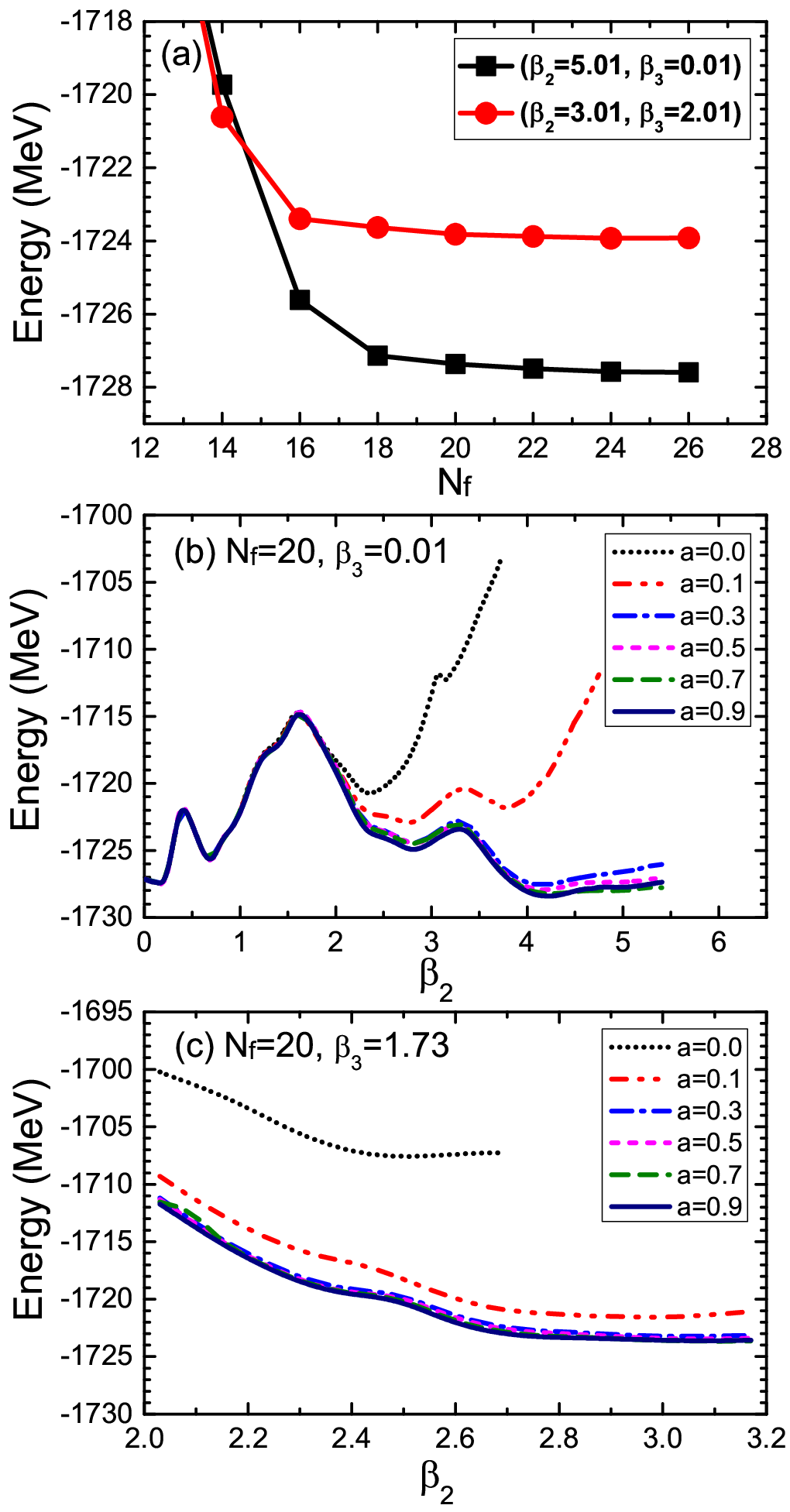
For a given number of shells and following the procedure described above, a larger value of the parameter in Eq. (28) implies an increase in the number of basis states and, consequently, longer computing times. The convergence check for different values of and is illustrated in Fig. 14. It is found that the choice of the above parameters largely mitigates basis truncation effects up to the scission point, where we estimate the error on the total energy to be MeV for and .
Acknowledgements.
This work was supported in part by the NSFC under Grant No. 11475140, the Croatian Science Foundation – project “Structure and Dynamics of Exotic Femtosystems” (IP-2014-09-9159), the QuantiXLie Centre of Excellence, the Chinese-Croatian project “Microscopic Energy Density Functionals Theory for Nuclear Fission”, and the NEWFELPRO project of the Ministry of Science, Croatia, co-financed through the Marie Curie FP7-PEOPLE-2011-COFUND program.References
- [1] N. Schunck and L. M. Robledo, Rep. Prog. Phys. 79, 116301 (2016).
- [2] Hans J. Krappe and K. Pomorski, Theory of Nuclear Fission (Springer-Verlag, Berlin Heidelberg, 2012).
- [3] Guillaume Scamps, Cédric Simenel, and Denis Lacroix, Phys. Rev. C 92, 011602(R) (2015).
- [4] C. Simenel and A. S. Umar, Phys. Rev. C 89, 031601(R) (2014).
- [5] P. Goddard, P. Stevenson, and A. Rios, Phys. Rev. C 92, 054610 (2015).
- [6] B. Avez, C. Simenel and P. Chomaz, Phys. Rev. C 78, 044318 (2008).
- [7] A. Bulgac, P. Magierski, K. J. Roche, and I. Stetcu, Phys. Rev. Lett. 116, 122504 (2016).
- [8] P. Goddard, P. Stevenson, and A. Rios, Phys. Rev. C 93, 014620 (2016).
- [9] Y. Tanimura, D. Lacroix, and S. Ayik, Phys. Rev. Lett. 118, 152501 (2017).
- [10] T. Nakatsukasa, K. Matsuyanagi, M. Matsuo, K. Yabana, Rev. Mod. Phys. 88, 045004 (2016).
- [11] S. A. Giuliani, L. M. Robledo, and R. Rodriguez-Guzman, Phys. Rev. C 90, 054311 (2014).
- [12] C. R. Chinn, J.-F. Berger, D. Gogny, and M. S. Weiss, Phys. Rev. C 45, 1700 (1992).
- [13] A. Staszczak, A. Baran, and W. Nazarewicz, Phys. Rev. C 87, 024320 (2013).
- [14] M. Warda and J. L. Egido, Phys. Rev. C 86, 014322 (2012).
- [15] J. W. Negele, Rev. Mod. Phys. 54, 913 (1982).
- [16] J. Sadhukhan, K. Mazurek, A. Baran, J. Dobaczewski, W. Nazarewicz, and J. A. Sheikh, Phys. Rev. C 88, 064314 (2013).
- [17] J. Sadhukhan, J. Dobaczewski, W. Nazarewicz, J. A. Sheikh, and A. Baran, Phys. Rev. C 90, 061304 (2014).
- [18] R. Smolańczuk, J. Skalski, and A. Sobiczewski, Phys. Rev. C 52,1871 (1995).
- [19] J. F. Berger, M. Girod, and D. Gogny, Comput. Phys. Comm. 63, 365 (1991).
- [20] H. Goutte, J. F. Berger, P. Casoli, and D. Gogny, Phys. Rev. C 71, 024316 (2005).
- [21] W. Younes and D. Gogny, Tech. Rep. LLNL-TR-586678 Lawrence Livermore National Laboratory (LLNL), Livermore, CA (2012).
- [22] D. Regnier, M. Verrière, N. Dubray, and N. Schunck, Comput. Phys. Commun. 200, 350 (2016).
- [23] D. Regnier, N. Dubray, N. Schunck, M. Verrière, Phys. Rev. C 93, 054611 (2016).
- [24] A. Zdeb, A. Dobrowolski, and M. Warda, Phys. Rev. C 95, 054608 (2017).
- [25] D. Vretenar, A. V. Afanasjev, G. A. Lalazissis, and P. Ring, Phys. Rep. 409, 101 (2005).
- [26] J. Meng, H. Toki, S. G. Zhou, S. Q. Zhang, W. H. Long, and L. S. Geng, Prog. Part. Nucl. Phys. 57, 470 (2006).
- [27] J. Stone and P.-G. Reinhard, Prog. Part. Nucl. Phys. 58, 587 (2007).
- [28] Relativistic Density Functional for Nuclear Structure, edited by J. Meng (World Scientific, Singapore, 2016).
- [29] Bing-Nan Lu, En-Guang Zhao, and Shan-Gui Zhou, Phys. Rev. C 85, 011301(R) (2012).
- [30] Z. P. Li, T. Nikšić, D. Vretenar, P. Ring, and J. Meng, Phys, Rev. C 81, 064321 (2010).
- [31] Bing-Nan Lu, Jie Zhao, En-Guang Zhao, and Shan-Gui Zhou, Phys. Rev. C 89, 014323 (2014).
- [32] Jie Zhao, Bing-Nan Lu, Dario Vretenar, En-Guang Zhao, and Shan-Gui Zhou, Phys. Rev. C 91, 014321 (2015).
- [33] J. Zhao, B. N. Lu, T. Nikšić, and D. Vretenar, Phys. Rev. C 92, 064315 (2015).
- [34] Jie Zhao, Bing-Nan Lu, Tamara Nikšić, Dario Vretenar, and Shan-Gui Zhou, Phys. Rev. C 93, 044315 (2016).
- [35] T. Burvenich, M. Bender, J. A. Maruhn, and P.-G. Reinhard, Phys. Rev. C 69, 014307 (2004).
- [36] V. Blum, J. Maruhn, P.-G. Reinhard, and W. Greiner, Phys. Lett. B 323, 262 (1994).
- [37] W. Zhang, S.-S. Zhang, S.-Q. Zhang, and J. Meng, Chin. Phys. Lett. 20, 1694 (2003).
- [38] M. Bender, P.-H. Heenen, and P.-G. Reinhard, Rev. Mod. Phys. 75, 121 (2003).
- [39] H.-F. Lu, L.-S. Geng, and J. Meng, Chin. Phys. Lett. 23, 2940 (2006).
- [40] H. Abusara, A. V. Afanasjev, and P. Ring, Phys. Rev. C 82, 044303 (2010).
- [41] H. Abusara, A. V. Afanasjev, and P. Ring, Phys. Rev. C 85, 024314 (2012).
- [42] S. E. Agbemava, A. V. Afanasjev, D. Ray, and P. Ring, Phys. Rev. C 95, 054324 (2017).
- [43] S.-G. Zhou, Phys. Scr. 91, 063008 (2016).
- [44] S. Karatzikos, A. Afanasjev, G. Lalazissis, and P. Ring, Phys. Lett. B 689, 72 (2010).
- [45] P. W. Zhao, Z. P. Li, J. M. Yao, and J. Meng, Phys. Rev. C 82, 054319 (2010).
- [46] P. Ring and P. Schuck, The Nuclear Many-Body Problem (Springer-Verlag, Heidelberg, 1980).
- [47] M. Girod and B. Grammaticos, Nucl. Phys. A 330, 40 (1979).
- [48] Z. P. Li, T. Nikšić and D. Vretenar, J. Phys. G: Nucl. Part. Phys. 43, 024005 (2016).
- [49] T. Nikšić, Z. P. Li, D. Vretenar, L. Próchniak, J. Meng, and P. Ring, Phys. Rev. C 79, 034303 (2009).
- [50] Z. P. Li, T. Nikšić, D. Vretenar, J. Meng, G. A. Lalazissis, and P. Ring, Phys. Rev. C 79, 054301 (2009).
- [51] D. R. Inglis, Phys.Rev. 103, 1786 (1956).
- [52] S. T. Belyaev, Nucl. Phys. 24, 322 (1961).
- [53] K.-H. Schmidt, S. Steinhauser, C. Bäckstiegel, A. Grewe, A. Heinz, A. R. Junghans, J. Benlliure, H.-G. Clerc, M. de Jong, J. M¡§uller, M. Pfützner, and B. Voss, Nucl. Phys. A 665, 221 (2001).
- [54] M. Bender, K. Rutz, P.-G. Reinhard, and J.A. Maruhn, Eur. Phys. J. A 8, 59-75 (2000).
- [55] N. Dubray, H. Goutte, and J.-P. Delaroche, Phys. Rev. C 77, 014310 (2008).
- [56] W. Younes and D. Gogny, Phys. Rev. C 80, 054313 (2009).
- [57] S. Pommé, E. Jacobs, M. Piessens, D. De Frenne, K. Persyn, K. Govaert, and M.-L. Yoneama, Nucl. Phys. A 572, 237 (1994).
- [58] N. Schunck, D. Duke, H. Carr, and A. Knoll, Phys. Rev. C 90, 054305 (2014).
- [59] D. E. Ward, B. G. Carlsson, T. Døssing, P. Möller, J. Randrup, and S. Åberg, Phys. Rev. C 95, 024618 (2017).
- [60] A. Baran, J. A. Sheikh, J. Dobaczewski, W. Nazarewicz, and A. Staszczak, Phys. Rev. C 84, 054321 (2011).
- [61] J. W. Negele, S. E. Koonin, P. Möller, J. R. Nix, and A. J. Sierk, Phys. Rev. C 17, 1098 (1978).
- [62] F. Barranco, G. F. Bertsch, R. A. Broglia, and E. Vigezzi, Nucl. Phys. A 512, 253 (1990).
- [63] G. F. Bertsch, Nucl. Phys. A 574, 169c (1994).
- [64] G. F. Bertsch and A. Bulgac, Phys. Rev. Lett. 79, 3539 (1997).
- [65] J. Sadhukhan, W. Nazarewicz and N. Schunck, Phys. Rev. C 93, 011304 (2016).