跳到论文正文
W Papers独立论文阅读器 arXiv:1708.03828 论文正文 计算阅读时间 · 0%
引用这篇论文根据当前论文元数据生成,正式投稿前建议核对。


License: arXiv.org perpetual non-exclusive license
arXiv:1708.03828v1 [math.OC] 12 Aug 2017

Balanced Truncation Model Reduction of Nonstationary Systems Interconnected over Arbitrary Graphs

Dany Abou Jaoude Affiliation: Kevin T. Crofton Department of Aerospace and Ocean Engineering, Virginia Tech, Blacksburg, VA 24061, U.S.A.    Mazen Farhood Affiliation: Email addresses: danyabj@vt.edu, farhood@vt.edu.
Abstract

This paper deals with the balanced truncation model reduction of discrete-time, linear time-varying, heterogeneous subsystems interconnected over finite arbitrary directed graphs. The information transfer between the subsystems is subject to a communication latency of one time-step. The presented method guarantees the preservation of the interconnection structure and further allows for its simplification. In addition to truncating temporal states associated with the subsystems, the method allows for the order reduction of spatial states associated with the interconnections between the subsystems and even the removal of whole interconnections. Upper bounds on the ℓ2\ell_{2}-induced norm of the resulting error system are derived. The proposed method is illustrated through an example.

Keywords: Model reduction, Interconnected systems, Linear systems, Time-varying systems, Directed graphs.

1 Introduction

Various biological and engineering systems consist of multiple interacting agents. Mathematically describing such systems can lead to models with a very large number of states, especially in the case of “large” models of the agents and complicated interconnection structures. Thus arises the need for model order reduction to simplify the control analysis and synthesis problems. Interconnected systems can be treated as one global system; and standard model reduction tools, like balanced truncation (BT) and coprime factors reduction (CFR), can then be applied to these systems. However, such an approach is not always desirable as it does not guarantee the preservation of the interconnection structure of the system.

Various works have addressed the problem of structure-preserving BT and CFR for interconnected systems. See, for example, Li and Paganini (2005); Sandberg and Murray (2009); Al-Taie and Werner (2016); Abou Jaoude and Farhood (2015); Abou Jaoude and Farhood (2016). The methods in these references, like the one in Beck et al. (1996), are based on the existence of block-diagonally structured solutions to linear matrix inequalities (LMIs). BT applies to stable systems, guarantees the stability of the reduced order system, and comes with a guaranteed upper bound on the norm of the error system. On the other hand, CFR applies to stabilizable and detectable systems, and guarantees the stabilizability and detectability of the reduced order system. However, the bound from CFR is not in terms of the norm of the error between the full and reduced order systems, but rather, it is in terms of the norm of the error between their corresponding coprime factorizations. The aforementioned works can be classified based on the modeling of the interconnections between the subsystems. Namely, Sandberg and Murray (2009) account for the interconnection structure using a transfer function matrix, whereas, Al-Taie and Werner (2016); Abou Jaoude and Farhood (2015); Abou Jaoude and Farhood (2016) model the interconnections between the subsystems as states, which we refer to as spatial states. The latter methods allow for the order reduction of the spatial states in addition to the standard states associated with the subsystems, which we refer to as the temporal states. That is, in addition to guaranteeing the preservation of the interconnection structure, these methods further allow for its simplification. In particular, Al-Taie and Werner (2016) deal with homogeneous, linear time-invariant (LTI) or linear parameter-varying (LPV) subsystems, interconnected over a grid. Model reduction is only applied to one subsystem, and then, all the temporal states, all the forward spatial states, and all the backward spatial states are truncated in a uniform way, respectively. As for Abou Jaoude and Farhood (2015); Abou Jaoude and Farhood (2016), they deal with heterogeneous, linear time-varying (LTV) subsystems, interconnected over arbitrary directed graphs. The methods therein allow for individually truncating each of the temporal and spatial states, and even permit the removal of a whole interconnection if it is deemed negligible. Due to the time-varying nature of the subsystems, these methods usually involve solving infinite sequences of LMIs. Also, if truncation is performed at infinitely many time-steps, the resulting error bound might not be finite. Abou Jaoude and Farhood (2015) show that in the special case of time-periodic subsystems, the sequences of LMIs can be restricted to the first time-period, and the error bound is guaranteed to be finite.

The current work extends the results of Abou Jaoude and Farhood (2015) from time-periodic subsystems to eventually time-periodic subsystems, i.e., subsystems which become time-periodic after some initial finite time-horizon. We also derive a tighter expression for the error bound for general LTV subsystems, which applies when the entries of the balanced gramians corresponding to the truncated states form monotonic sequences in time. We also provide an illustrative example.

The paper is organized as follows. In Section 2, we define the notation and summarize the adopted state-space framework along with the relevant analysis results. Then, in Section 3, we present the BT method. We derive the error bounds in Section 4 and treat the special class of eventually time-periodic subsystems in Section 5. In Section 6, we apply the method to an example. We conclude the paper with Section 7.

2 Preliminaries

2.1 Notation

Refer to caption
Figure 1: Example of a directed graph.

The sets of nonnegative integers, real numbers, and n×nn\times n symmetric matrices are denoted by ℕ0\mathbb{N}_{0}, ℝ\mathbb{R}, and 𝕊n\mathbb{S}^{n}, respectively. Let SS be an ordered subset of ℕ0\mathbb{N}_{0}. We denote by (vi)i∈S(v_{i})_{i\in S} the vector-valued sequence associated with SS and by vec​(vi)i∈S\mbox{vec}(v_{i})_{i\in S} the vertical concatenation of the elements of (vi)i∈S(v_{i})_{i\in S}. The elements in (vi)i∈S(v_{i})_{i\in S} are ordered conformably with the elements in SS. As an example, let S={1,2,4}S=\{1,2,4\}. Then, (vi)i∈S=(v1,v2,v4)(v_{i})_{i\in S}=(v_{1},v_{2},v_{4}) and vec​(vi)i∈S=[v1Tv2Tv4T]T\mbox{vec}(v_{i})_{i\in S}=\begin{bmatrix}v_{1}^{T}&v_{2}^{T}&v_{4}^{T}\end{bmatrix}^{T}. Similarly, we denote by (Mi)i∈S(M_{i})_{i\in S} the matrix-valued sequence associated with SS and by diag​(Mi)i∈S\mathrm{diag}(M_{i})_{i\in S} the block-diagonal augmentation of the elements of (Mi)i∈S(M_{i})_{i\in S}. In our example, (Mi)i∈S=(M1,M2,M4)(M_{i})_{i\in S}=(M_{1},M_{2},M_{4}) and diag​(Mi)i∈S=diag⁡(M1,M2,M4)=[M1000M2000M4]\mathrm{diag}(M_{i})_{i\in S}=\mathrm{diag}(M_{1},M_{2},M_{4})=\begin{bmatrix}M_{1}&0&0\\ 0&M_{2}&0\\ 0&0&M_{4}\end{bmatrix}. 0i×j0_{i\times j} denotes an i×ji\times j zero matrix and IiI_{i} denotes an i×ii\times i identity matrix.

𝒢⁡(V,E)\mathcal{G}(V,E) refers to a directed graph with set of vertices VV and set of directed edges EE. We assume throughout that the directed graph under consideration is finite. That is, both VV and EE are finite sets. We denote by NN the finite number of vertices, and choose V={1,…,N}V=\{1,\ldots,N\}. The ordered pair (i,j)(i,j) is in EE if there exists a directed edge from i∈Vi\in V to j∈Vj\in V. For each k∈Vk\in V, we define the set of vertices with an outgoing edge to kk as Ein(k)={i∈V|(i,k)∈E}E_{{\rm{in}}}^{(k)}=\{i\in V\,|\,(i,k)\in E\}, and denote its cardinality by m⁡(k)m(k). Similarly, we define the set of vertices with an incoming edge from kk as Eout(k)={j∈V|(k,j)∈E}E_{{\rm{out}}}^{(k)}=\{j\in V\,|\,(k,j)\in E\}, and denote its cardinality by p⁡(k)p(k). We order the elements in these sets in an increasing fashion. For example, consider the directed graph in Figure 1. For k=1k=1, we define Ein(1)={2,3,4}E_{{\rm{in}}}^{(1)}=\{2,3,4\}, m⁡(1)=3m(1)=3, Eout(1)={2,3,5}E_{{\rm{out}}}^{(1)}=\{2,3,5\}, p⁡(1)=3p(1)=3, and so on.

X≺0X\prec 0 (resp. ≻0\succ 0) means that the symmetric matrix XX is negative definite (resp. positive definite). Let nn be an integer sequence such that n:(t,k)∈ℕ0×Vn:(t,k)\in\mathbb{N}_{0}\times V →n(k)​(t)∈ℕ0\rightarrow n^{(k)}(t)\in\mathbb{N}_{0}. We define ℓ⁡({ℝn(k)​(t)})\ell(\{\mathbb{R}^{n^{(k)}(t)}\}) as the vector space of mappings w:(t,k)∈ℕ0×V→w(k)​(t)∈ℝn(k)​(t)w:(t,k)\in\mathbb{N}_{0}\times V\rightarrow w^{(k)}(t)\in\mathbb{R}^{n^{(k)}(t)}. The Hilbert space ℓ2​({ℝn(k)​(t)})\ell_{2}(\{\mathbb{R}^{n^{(k)}(t)}\}) is the subspace of ℓ⁡({ℝn(k)​(t)})\ell(\{\mathbb{R}^{n^{(k)}(t)}\}) consisting of mappings ww with a finite ℓ2\ell_{2}-norm ‖w‖2=(∑(t,k)w(k)​(t)T​w(k)​(t))12\|w\|_{2}=\left(\sum_{(t,k)}w^{(k)}(t)^{T}w^{(k)}(t)\right)^{\frac{1}{2}}. We subsequently use the abbreviated symbols ℓ\ell and ℓ2\ell_{2}.

2.2 State-Space Representation

Next, we give the state-space equations for a distributed system GG, formed by discrete-time, heterogeneous, LTV subsystems interconnected over finite arbitrary directed graphs and subjected to a communication latency. We represent the interconnection structure of GG using a directed graph 𝒢⁡(V,E)\mathcal{G}(V,E), where each subsystem G(k)G^{(k)} corresponds to a vertex k∈Vk\in V, and the interconnections between the subsystems are described by the directed edges. Each subsystem G(k)G^{(k)} has a discrete-time LTV model, with states x(k)​(t)x^{(k)}(t), inputs u(k)​(t)u^{(k)}(t), and outputs y(k)​(t)y^{(k)}(t). We refer to the states associated with the subsystems as temporal states or vertex/node states. The interconnections between the subsystems are also modeled using states, which we refer to as spatial states or interconnection/edge states. Namely, we associate a state x(i​j)​(t)x^{(ij)}(t) with each edge (i,j)∈E(i,j)\in E. Due to the communication latency, the information sent from G(i)G^{(i)} at time tt reaches G(j)G^{(j)} at the next time-step, i.e., t+1t+1. For each subsystem G(k)G^{(k)}, we define vectors xin(k)​(t)=vec​(x(i​k)​(t))i∈Ein(k)x_{{\rm{in}}}^{(k)}(t)=\mbox{vec}(x^{(ik)}(t))_{i\in E_{{\rm{in}}}^{(k)}} and xout(k)​(t)=vec​(x(k​j)​(t))j∈Eout(k)x_{{\rm{out}}}^{(k)}(t)=\mbox{vec}(x^{(kj)}(t))_{j\in E_{{\rm{out}}}^{(k)}}, which are partitioned into m⁡(k)m(k) and p⁡(k)p(k) vector-valued channels, respectively. These vectors represent the total information received and sent by G(k)G^{(k)} at time tt. When all subsystems are considered, and since the interconnection input to a subsystem is an output to another subsystem, both xout(k)x^{(k)}_{{\rm{out}}} and xin(k)x^{(k)}_{{\rm{in}}} contain all spatial states x(i​j)x^{(ij)}. We assume zero initial conditions for the temporal and the spatial states. Then, for all (t,k)∈ℕ0×V(t,k)\in\mathbb{N}_{0}\times V, we have x(k)​(0)=0x^{(k)}(0)=0, xin(k)​(0)=0x_{{\rm{in}}}^{(k)}(0)=0,

[x(k)​(t+1)xout(k)​(t+1)]\displaystyle\begin{bmatrix}x^{(k)}(t+1)\\ x_{{\rm{out}}}^{(k)}(t+1)\end{bmatrix} =A(k)​(t)​[x(k)​(t)xin(k)​(t)]+B(k)​(t)​u(k)​(t),\displaystyle=A^{(k)}(t)\begin{bmatrix}x^{(k)}(t)\\ x_{{\rm{in}}}^{(k)}(t)\end{bmatrix}+B^{(k)}(t)\,u^{(k)}(t),
y(k)​(t)\displaystyle y^{(k)}(t) =C(k)​(t)​[x(k)​(t)xin(k)​(t)]+D(k)​(t)​u(k)​(t).\displaystyle=C^{(k)}(t)\begin{bmatrix}x^{(k)}(t)\\ x_{{\rm{in}}}^{(k)}(t)\end{bmatrix}+D^{(k)}(t)\,u^{(k)}(t). (1)

The matrix-valued sequences of state-space matrices, e.g., A(k)​(t)A^{(k)}(t), are known a priori and assumed to be uniformly bounded. The dimensions of signals x(k)​(t)x^{(k)}(t), u(k)​(t)u^{(k)}(t), y(k)​(t)y^{(k)}(t), and x(i​j)​(t)x^{(ij)}(t) can vary with tt, and kk or (i,j)(i,j), and are denoted by n(k)​(t),nu(k)​(t)n^{(k)}(t),n_{u}^{(k)}(t), ny(k)​(t)n_{y}^{(k)}(t), and n(i​j)​(t)n^{(ij)}(t), respectively, for all (t,k)∈ℕ0×V(t,k)\in\mathbb{N}_{0}\times V and (i,j)∈E(i,j)\in E. We denote the realization of system GG by the quadruple (A(k)​(t),B(k)​(t),C(k)​(t),D(k)​(t))\left(A^{(k)}(t),B^{(k)}(t),C^{(k)}(t),D^{(k)}(t)\right).

For each (t,k)(t,k), the state-space matrices are naturally partitioned conformably with the partitioning of [x(k)​(t+1)Txout(k)​(t+1)T]T\begin{bmatrix}x^{(k)}(t+1)^{T}&x_{{\rm{out}}}^{(k)}(t+1)^{T}\end{bmatrix}^{T} and [x(k)​(t)Txin(k)​(t)T]T\begin{bmatrix}x^{(k)}(t)^{T}&x_{{\rm{in}}}^{(k)}(t)^{T}\end{bmatrix}^{T}. For example, consider the distributed system in Figure 1. The state-space matrices of subsystem G(1)G^{(1)} are partitioned as follows:

A(1)​(t)=[​A00(1)​(t)A02(1)​(t)A03(1)​(t)A04(1)​(t)​A20(1)​(t)A22(1)​(t)A23(1)​(t)A24(1)​(t)​A30(1)​(t)A32(1)​(t)A33(1)​(t)A34(1)​(t)​A50(1)​(t)A52(1)​(t)A53(1)​(t)A54(1)​(t)],B(1)​(t)=[​B0(1)​(t)​B2(1)​(t)​B3(1)​(t)​B5(1)​(t)],C(1)​(t)=[C0(1)​(t)C2(1)​(t)C3(1)​(t)C4(1)​(t)],A^{(1)}(t){=}\!\begin{bmatrix}\rule{0.0pt}{12.80373pt}A_{00}^{(1)}(t)&\!\!A_{02}^{(1)}(t)&\!\!A_{03}^{(1)}(t)&\!\!A_{04}^{(1)}(t)\\ \rule{0.0pt}{12.80373pt}A_{20}^{(1)}(t)&\!\!A_{22}^{(1)}(t)&\!\!A_{23}^{(1)}(t)&\!\!A_{24}^{(1)}(t)\\ \rule{0.0pt}{12.80373pt}A_{30}^{(1)}(t)&\!\!A_{32}^{(1)}(t)&\!\!A_{33}^{(1)}(t)&\!\!A_{34}^{(1)}(t)\\ \rule{0.0pt}{12.80373pt}A_{50}^{(1)}(t)&\!\!A_{52}^{(1)}(t)&\!\!A_{53}^{(1)}(t)&\!\!A_{54}^{(1)}(t)\end{bmatrix}\!\!{,}\,\,B^{(1)}(t){=}\!\begin{bmatrix}\rule{0.0pt}{12.80373pt}B_{0}^{(1)}(t)\\ \rule{0.0pt}{12.80373pt}B_{2}^{(1)}(t)\\ \rule{0.0pt}{12.80373pt}B_{3}^{(1)}(t)\\ \rule{0.0pt}{12.80373pt}B_{5}^{(1)}(t)\end{bmatrix}\!\!{,}\,\,C^{(1)}(t){=}\!\begin{bmatrix}C_{0}^{(1)}(t)&\!\!C_{2}^{(1)}(t)&\!\!C_{3}^{(1)}(t)&\!\!C_{4}^{(1)}(t)\end{bmatrix}\!\!{,}

where A00(1)​(t)A_{00}^{(1)}(t) is an n(1)​(t+1)×n(1)​(t)n^{(1)}(t+1)\times n^{(1)}(t) matrix, A20(1)​(t)A_{20}^{(1)}(t) is an n(12)​(t+1)×n(1)​(t)n^{(12)}(t+1)\times n^{(1)}(t) matrix, B0(1)​(t)B_{0}^{(1)}(t) is an n(1)​(t+1)×nu(1)​(t)n^{(1)}(t+1)\times n_{u}^{(1)}(t) matrix, C0(1)​(t)C_{0}^{(1)}(t) is an ny(1)​(t)×n(1)​(t)n_{y}^{(1)}(t)\times n^{(1)}(t) matrix, C2(1)​(t)C_{2}^{(1)}(t) is an ny(1)​(t)×n(21)​(t)n_{y}^{(1)}(t)\times n^{(21)}(t) matrix, etc.

2.3 Analysis Results

We now summarize the relevant analysis results of Farhood et al. (2015). We consider a system GG with realization (A(k)​(t),B(k)​(t),C(k)​(t),D(k)​(t))(A^{(k)}(t),B^{(k)}(t),C^{(k)}(t),D^{(k)}(t)). Since the state-space equations (1) have zero initial conditions and the state-space matrices are defined for t∈ℕ0t\in\mathbb{N}_{0}, we can equivalently assume that the state-space matrices are zeros for t<0t<0. Then, from Dullerud and DflAndrea (2004), it can be shown that system GG is well-posed, i.e., given inputs in ℓ\ell, the state-space equations admit unique solutions in ℓ\ell, and further define a linear causal mapping on ℓ\ell. A well-posed system GG is said to be stable if, given inputs in ℓ2\ell_{2}, the state-space equations admit unique solutions in ℓ2\ell_{2}, and further define a linear causal mapping on ℓ2\ell_{2}. Next, we give a Lyapunov-based test to check if system GG is stable. The result constitutes the basis of the BT method.

Lemma 1.

System GG is stable if there exist β>0\beta>0 and uniformly bounded, positive definite, matrix-valued functions X(k)​(t)∈𝕊n(k)​(t)X^{(k)}(t)\in\mathbb{S}^{n^{(k)}(t)} and X(i​j)​(t)∈𝕊n(i​j)​(t)X^{(ij)}(t)\in\mathbb{S}^{n^{(ij)}(t)}, for all (t,k)∈ℕ0×V(t,k)\in\mathbb{N}_{0}\times V and (i,j)∈E(i,j)\in E, such that X(k)​(t)≻β​IX^{(k)}(t)\succ\beta I, X(i​j)​(t)≻β​IX^{(ij)}(t)\succ\beta I, and

A(k)​(t)T​[X(k)​(t+1)00Xout(k)​(t+1)]​A(k)​(t)−[X(k)​(t)00Xin(k)​(t)]≺−β​I,A^{(k)}(t)^{T}\begin{bmatrix}X^{(k)}(t+1)&0\\ 0&X_{{\rm{out}}}^{(k)}(t+1)\end{bmatrix}A^{(k)}(t)-\begin{bmatrix}X^{(k)}(t)&0\\ 0&X_{{\rm{in}}}^{(k)}(t)\end{bmatrix}\prec-\beta I, (2)
Xin(k)​(t)=diag​(X(i​k)​(t))i∈Ein(k),andXout(k)​(t)=diag​(X(k​j)​(t))j∈Eout(k).X_{{\rm{in}}}^{(k)}(t)=\mathrm{diag}(X^{(ik)}(t))_{i\in E_{{\rm{in}}}^{(k)}},\quad\quad\mbox{and}\quad\quad X_{{\rm{out}}}^{(k)}(t)=\mathrm{diag}(X^{(kj)}(t))_{j\in E_{{\rm{out}}}^{(k)}}.

The solutions to (2) can be classified into temporal terms X(k)​(t)X^{(k)}(t) and spatial terms X(i​j)​(t)X^{(ij)}(t). Due to the time-varying nature of the subsystems, there is an infinite sequence of LMIs associated with each subsystem. Moreover, the LMI sequence associated with a given subsystem is coupled with the LMI sequences of the other subsystems through the spatial terms. The “β​I\beta I” terms in (2) are small quantities added to ensure that the matrix sequences on the left-hand side do not converge to singular matrices as tt approaches infinity. Note that the conditions X(k)​(t)≻β​IX^{(k)}(t)\succ\beta I and X(i​j)​(t)≻β​IX^{(ij)}(t)\succ\beta I are implied by (2). Even though redundant, these conditions are explicitly given in the statement of the lemma to stress that the terms X(k)​(t)X^{(k)}(t) and X(i​j)​(t)X^{(ij)}(t) do not approach singular matrices as tt approaches infinity, as explained above. Uniform positive definiteness will be used in due course to guarantee the invertibility and the boundedness of the inverses of such terms. Subsequently, we no longer specify the dimensions of X(k)​(t)X^{(k)}(t) and X(i​j)​(t)X^{(ij)}(t).

Systems that satisfy the conditions in Lemma 1 are called strongly stable. Lemma 1 provides a sufficient condition for stability, and so strong stability implies stability, but the converse is not always true. Specifically, strongly stable systems are stable systems which have the required structured solutions to (2). The proposed BT scheme suffers from conservatism as it only applies to strongly stable systems. However, this imposed structure on the solutions of (2) allows for the preservation and the simplification of the interconnection structure during the model reduction process. Trnka et al. (2013); Sootla and Anderson (2016) identify classes of systems with guaranteed structured solutions to LMIs.

For a stable system GG mapping u∈ℓ2u\in\ell_{2} to y∈ℓ2y\in\ell_{2} and starting from zero initial conditions, the ℓ2\ell_{2}-induced norm is defined as ‖G‖=sup0≠u∈ℓ2‖y‖2‖u‖2\|G\|=\sup_{0\neq u\in\ell_{2}}\frac{\|y\|_{2}}{\|u\|_{2}}.

Lemma 2.

System GG is strongly stable and satisfies ‖G‖<γ\|G\|<\gamma, for some γ>0\gamma>0, if there exist β>0\beta>0 and uniformly bounded, positive definite, matrix-valued functions X(k)​(t)≻β​IX^{(k)}(t)\succ\beta I and X(i​j)​(t)≻β​IX^{(ij)}(t)\succ\beta I, for all (t,k)∈ℕ0×V(t,k)\in\mathbb{N}_{0}\times V and (i,j)∈E(i,j)\in E, such that

[A(k)​(t)B(k)​(t)C(k)​(t)D(k)​(t)]T​[X(k)​(t+1)000Xout(k)​(t+1)000I]​[A(k)​(t)B(k)​(t)C(k)​(t)D(k)​(t)]−[X(k)​(t)000Xin(k)​(t)000γ2​I]≺−β​I.\begin{bmatrix}A^{(k)}(t)&B^{(k)}(t)\\ C^{(k)}(t)&D^{(k)}(t)\end{bmatrix}^{T}\begin{bmatrix}X^{(k)}(t+1)&0&0\\ 0&X_{{\rm{out}}}^{(k)}(t+1)&0\\ 0&0&I\end{bmatrix}\begin{bmatrix}A^{(k)}(t)&B^{(k)}(t)\\ C^{(k)}(t)&D^{(k)}(t)\end{bmatrix}-\begin{bmatrix}X^{(k)}(t)&0&0\\ 0&X_{{\rm{in}}}^{(k)}(t)&0\\ 0&0&\gamma^{2}I\end{bmatrix}\prec-\beta I. (3)

3 Balanced Truncation Model Reduction

3.1 Balanced Realization

We now extend the notions of generalized Lyapunov inequalities and generalized gramians, discussed in Hinrichsen and Pritchard (1990); Beck et al. (1996), to the class of distributed systems. Namely, the controllability and observability generalized gramians are uniformly bounded, positive definite, matrix-valued functions, denoted by X(k)​(t)X^{(k)}(t), X(i​j)​(t)X^{(ij)}(t) and Y(k)​(t)Y^{(k)}(t), Y(i​j)​(t)Y^{(ij)}(t), respectively, which, for some scalar β>0\beta>0, satisfy X(k)​(t)≻β​IX^{(k)}(t)\succ\beta I, X(i​j)​(t)≻β​IX^{(ij)}(t)\succ\beta I and Y(k)​(t)≻β​IY^{(k)}(t)\succ\beta I, Y(i​j)​(t)≻β​IY^{(ij)}(t)\succ\beta I, in addition to the following generalized Lyapunov inequalities:

A(k)​(t)​[X(k)​(t)00Xin(k)​(t)]​A(k)​(t)T−[X(k)​(t+1)00Xout(k)​(t+1)]+B(k)​(t)​B(k)​(t)T≺−β​I,\displaystyle A^{(k)}(t)\begin{bmatrix}X^{(k)}(t)&0\\ 0&X_{{\rm{in}}}^{(k)}(t)\end{bmatrix}A^{(k)}(t)^{T}-\begin{bmatrix}X^{(k)}(t+1)&0\\ 0&X_{{\rm{out}}}^{(k)}(t+1)\end{bmatrix}+B^{(k)}(t)B^{(k)}(t)^{T}\prec-\beta I, (4)
A(k)​(t)T​[Y(k)​(t+1)00Yout(k)​(t+1)]​A(k)​(t)−[Y(k)​(t)00Yin(k)​(t)]+C(k)​(t)T​C(k)​(t)≺−β​I,\displaystyle A^{(k)}(t)^{T}\begin{bmatrix}Y^{(k)}(t+1)&0\\ 0&Y_{{\rm{out}}}^{(k)}(t+1)\end{bmatrix}A^{(k)}(t)-\begin{bmatrix}Y^{(k)}(t)&0\\ 0&Y_{{\rm{in}}}^{(k)}(t)\end{bmatrix}+C^{(k)}(t)^{T}C^{(k)}(t)\prec-\beta I, (5)

where Yin(k)​(t)Y_{{\rm{in}}}^{(k)}(t) and Yout(k)​(t)Y_{{\rm{out}}}^{(k)}(t) are defined similarly to Xin(k)​(t)X_{{\rm{in}}}^{(k)}(t) and Xout(k)​(t)X_{{\rm{out}}}^{(k)}(t). The generalized Lyapunov inequalities and the generalized gramians allow for the definition of a balanced realization of a distributed system as given next.

Definition 1.

The realization of system GG is said to be balanced if there exist β>0\beta>0 and uniformly bounded, diagonal, positive definite, matrix-valued functions Σ(k)​(t)≻β​I\Sigma^{(k)}(t)\succ\beta I and Σ(i​j)​(t)≻β​I\Sigma^{(ij)}(t)\succ\beta I, for all (t,k)∈ℕ0×V(t,k)\in\mathbb{N}_{0}\times V and (i,j)∈E(i,j)\in E, that simultaneously satisfy (4) and (5), i.e., Σ(k)​(t)=X(k)​(t)=Y(k)​(t)\Sigma^{(k)}(t)=X^{(k)}(t)=Y^{(k)}(t), Σ(i​j)​(t)=X(i​j)​(t)=Y(i​j)​(t)\Sigma^{(ij)}(t)=X^{(ij)}(t)=Y^{(ij)}(t), and Σ(k)​(t)\Sigma^{(k)}(t) and Σ(i​j)​(t)\Sigma^{(ij)}(t) are diagonal matrices.

We can show (see the proof of Theorem 4) that the existence of solutions to (2) is equivalent to the existence of solutions to (4) and (5), respectively. Thus, the generalized gramians are only defined for strongly stable systems. These gramians can be used to construct a balanced realization and balanced generalized gramians Σ(k)​(t)\Sigma^{(k)}(t), Σ(i​j)​(t)\Sigma^{(ij)}(t) for a given system GG, as outlined next.

Algorithm 1.

We construct a balanced realization for a given strongly stable system GG with generalized gramians X(k)​(t)X^{(k)}(t), X(i​j)​(t)X^{(ij)}(t) and Y(k)​(t)Y^{(k)}(t), Y(i​j)​(t)Y^{(ij)}(t) as follows. First, we compute the Cholesky factorizations

X(k)​(t)=R(k)​(t)T​R(k)​(t)andY(k)​(t)=H(k)​(t)T​H(k)​(t),X^{(k)}(t)=R^{(k)}(t)^{T}R^{(k)}(t)\quad\quad\mbox{and}\quad\quad Y^{(k)}(t)=H^{(k)}(t)^{T}H^{(k)}(t),

and we perform the singular value decompositions

H(k)​(t)​R(k)​(t)T=U(k)​(t)​Σ(k)​(t)​V(k)​(t)T.H^{(k)}(t)R^{(k)}(t)^{T}=U^{(k)}(t)\Sigma^{(k)}(t)V^{(k)}(t)^{T}.

Then, we define the balancing transformations

T(k)(t)=Σ(k)(t)−1/2U(k)(t)TH(k)(t)andT(k)(t)−1=R(k)(t)TV(k)(t)Σ(k)(t)−1/2.T^{(k)}(t)=\Sigma^{(k)}(t)^{-1/2}\,\,U^{(k)}(t)^{T}\,\,H^{(k)}(t)\quad\quad\mbox{and}\quad\quad T^{(k)}(t)^{-1}=R^{(k)}(t)^{T}\,\,V^{(k)}(t)\,\,\Sigma^{(k)}(t)^{-1/2}.

Similar steps are repeated for the spatial terms. Σ(k)​(t)\Sigma^{(k)}(t), Σ(i​j)​(t)\Sigma^{(ij)}(t) are the balanced generalized gramians. We augment the obtained transformations as in

Tpre(k)​(t)=diag⁡(T(k)​(t),Tout(k)​(t)),andTpost(k)​(t)=diag⁡(T(k)​(t)−1,Tin(k)​(t)−1).T_{{\rm{pre}}}^{(k)}(t)=\mathrm{diag}(T^{(k)}(t),T_{{\rm{out}}}^{(k)}(t)),\quad\quad\mbox{and}\quad\quad T_{{\rm{post}}}^{(k)}(t)=\mathrm{diag}(T^{(k)}(t)^{-1},T_{{\rm{in}}}^{(k)}(t)^{-1}).

A balanced realization (Abal(k)​(t),Bbal(k)​(t),Cbal(k)​(t),D(k)​(t))(A_{{\rm{bal}}}^{(k)}(t),B_{{\rm{bal}}}^{(k)}(t),C_{{\rm{bal}}}^{(k)}(t),D^{(k)}(t)) of GG is then given by

Abal(k)(t)=Tpre(k)(t+1)A(k)(t)Tpost(k)(t),Bbal(k)(t)=Tpre(k)(t+1)B(k)(t),andCbal(k)(t)=C(k)(t)Tpost(k)(t).A_{{\rm{bal}}}^{(k)}(t)=T_{{\rm{pre}}}^{(k)}(t+1)A^{(k)}(t)T_{{\rm{post}}}^{(k)}(t),\quad B_{{\rm{bal}}}^{(k)}(t)=T_{{\rm{pre}}}^{(k)}(t+1)B^{(k)}(t),\quad\mbox{and}\quad C_{{\rm{bal}}}^{(k)}(t)=C^{(k)}(t)T_{{\rm{post}}}^{(k)}(t).

An alternative algorithm is also given in Abou Jaoude and Farhood (2015). Clearly, the balanced realization of a strongly stable system is not unique as it depends on the followed algorithm as well as the solutions to (4) and (5) used in the algorithm. To obtain useful results for model reduction, namely entries in the balanced generalized gramians that yield reasonable error bounds, we use a trace heuristic, i.e., we find generalized gramians with minimum sum of traces, see e.g., Farhood and Dullerud (2007) and Farhood and Beck (2014). An alternative heuristic is proposed in Al-Taie and Werner (2016).

3.2 Balanced Truncation

Let GG be a distributed system with a balanced realization (A(k)​(t),B(k)​(t),C(k)​(t),D(k)​(t))\left(A^{(k)}(t),B^{(k)}(t),C^{(k)}(t),D^{(k)}(t)\right). We assume, without loss of generality, that the diagonal entries of the balanced generalized gramians are ordered in a decreasing fashion. The essence of BT is to truncate the state variables associated with the negligible entries. We partition the gramians into two blocks: one corresponding to the non-truncated states and the other to the truncated states. We illustrate the partitioning process for the temporal terms. Given integers r(k)​(t)r^{(k)}(t), such that 0≤r(k)​(t)≤n(k)​(t)0\leq r^{(k)}(t)\leq n^{(k)}(t), we partition Σ(k)​(t)\Sigma^{(k)}(t) as Σ(k)​(t)=diag⁡(Γ(k)​(t),Ω(k)​(t))\Sigma^{(k)}(t)=\mathrm{diag}(\Gamma^{(k)}(t),\,\Omega^{(k)}(t)), where Γ(k)​(t)∈𝕊r(k)​(t)\Gamma^{(k)}(t)\in\mathbb{S}^{r^{(k)}(t)} are reduced order gramians associated with the non-truncated states and Ω(k)​(t)\Omega^{(k)}(t) correspond to the truncated states. By allowing r(k)​(t)r^{(k)}(t) to be equal to 00 or n(k)​(t)n^{(k)}(t) for some (t,k)(t,k), we allow that either all or no variables be truncated from the corresponding temporal state x(k)​(t)x^{(k)}(t). This results in either Γ(k)​(t)\Gamma^{(k)}(t) or Ω(k)​(t)\Omega^{(k)}(t) having a zero dimension, which is a slight abuse of notation. The proposed method allows for the evaluation of the importance of a particular interconnection, and accordingly, the reduction of the dimension of the spatial state vector associated with it and even the complete removal of the interconnection. For example, if r(i​j)​(t)=0r^{(ij)}(t)=0, for all t∈ℕ0t\in\mathbb{N}_{0}, then the edge (i,j)(i,j) is removed altogether from the interconnection structure.

The next step is to partition the blocks of the state-space matrices in accordance with the partitioning of the blocks of diag⁡(Σ(k)​(t+1),Σout(k)​(t+1))\mathrm{diag}(\Sigma^{(k)}(t+1),\Sigma_{{\rm{out}}}^{(k)}(t+1)) and diag⁡(Σ(k)​(t),Σin(k)​(t))\mathrm{diag}(\Sigma^{(k)}(t),\Sigma_{{\rm{in}}}^{(k)}(t)). Consider subsystem G(1)G^{(1)} in Figure 1. A00(1)​(t)A_{00}^{(1)}(t) is partitioned according to the partitioning of Σ(1)​(t+1)=diag⁡(Γ(1)​(t+1),Ω(1)​(t+1))\Sigma^{(1)}(t+1)=\mathrm{diag}(\Gamma^{(1)}(t+1),\,\Omega^{(1)}(t+1)) and Σ(1)​(t)=diag⁡(Γ(1)​(t),Ω(1)​(t))\Sigma^{(1)}(t)=\mathrm{diag}(\Gamma^{(1)}(t),\,\Omega^{(1)}(t)) as in

A00(1)​(t)=[A^00(1)​(t)A0012(1)​(t)A0021(1)​(t)A0022(1)​(t)], where A^00(1)​(t) is an r(1)​(t+1)×r(1)​(t) matrix.A_{00}^{(1)}(t)=\begin{bmatrix}\hat{A}_{00}^{(1)}(t)&A_{00_{12}}^{(1)}(t)\\ A_{00_{21}}^{(1)}(t)&A_{00_{22}}^{(1)}(t)\end{bmatrix},\mbox{ where $\hat{A}_{00}^{(1)}(t)$ is an $r^{(1)}(t+1){\times}r^{(1)}(t)$ matrix.}

B0(1)​(t)B_{0}^{(1)}(t) is partitioned conformably with the partitioning of Σ(1)​(t+1)=diag⁡(Γ(1)​(t+1),Ω(1)​(t+1))\Sigma^{(1)}(t+1)=\mathrm{diag}(\Gamma^{(1)}(t+1),\,\Omega^{(1)}(t+1)) as in

B0(1)​(t)=[B^0(1)​(t)B02(1)​(t)], where B^0(1)​(t) is an r(1)​(t+1)×nu(1)​(t) matrix.B_{0}^{(1)}(t)=\begin{bmatrix}\hat{B}_{0}^{(1)}(t)\\ B_{0_{2}}^{(1)}(t)\end{bmatrix},\mbox{ where $\hat{B}_{0}^{(1)}(t)$ is an $r^{(1)}(t+1){\times}n_{u}^{(1)}(t)$ matrix.}

Likewise, C0(1)​(t)C_{0}^{(1)}(t) is partitioned according to the partitioning of Σ(1)​(t)=diag⁡(Γ(1)​(t),Ω(1)​(t))\Sigma^{(1)}(t)=\mathrm{diag}(\Gamma^{(1)}(t),\,\Omega^{(1)}(t)), namely,

C0(1)​(t)=[C^0(1)​(t)C02(1)​(t)], where C^0(1)​(t) is an ny(1)​(t)×r(1)​(t) matrix, and so on.C_{0}^{(1)}(t)=\begin{bmatrix}\hat{C}_{0}^{(1)}(t)&C_{0_{2}}^{(1)}(t)\end{bmatrix},\mbox{ where $\hat{C}_{0}^{(1)}(t)$ is an $n_{y}^{(1)}(t)\times r^{(1)}(t)$ matrix, and so on.}

Now, we form the realization (Ar(k)​(t),Br(k)​(t),Cr(k)​(t),D(k)​(t))(A_{r}^{(k)}(t),B_{r}^{(k)}(t),C_{r}^{(k)}(t),D^{(k)}(t)) of the reduced order system GrG_{r}. For Ar(k)​(t)A_{r}^{(k)}(t), Br(k)​(t)B_{r}^{(k)}(t), and Cr(k)​(t)C_{r}^{(k)}(t), we keep the blocks that correspond to the non-truncated states, i.e., the partitions marked with a hat, e.g., Cr(1)​(t)=[C^0(1)​(t)C^2(1)​(t)C^3(1)​(t)C^4(1)​(t)]C_{r}^{(1)}(t)=\begin{bmatrix}\hat{C}_{0}^{(1)}(t)&\hat{C}_{2}^{(1)}(t)&\hat{C}_{3}^{(1)}(t)&\hat{C}_{4}^{(1)}(t)\end{bmatrix},

Ar(1)​(t)=[​A^00(1)​(t)A^02(1)​(t)A^03(1)​(t)A^04(1)​(t)​A^20(1)​(t)A^22(1)​(t)A^23(1)​(t)A^24(1)​(t)​A^30(1)​(t)A^32(1)​(t)A^33(1)​(t)A^34(1)​(t)​A^50(1)​(t)A^52(1)​(t)A^53(1)​(t)A^54(1)​(t)],andBr(1)​(t)=[B^0(1)​(t)​B^2(1)​(t)​B^3(1)​(t)​B^5(1)​(t)].A_{r}^{(1)}(t)=\begin{bmatrix}\rule{0.0pt}{14.22636pt}\hat{A}_{00}^{(1)}(t)&\hat{A}_{02}^{(1)}(t)&\hat{A}_{03}^{(1)}(t)&\hat{A}_{04}^{(1)}(t)\\ \rule{0.0pt}{14.22636pt}\hat{A}_{20}^{(1)}(t)&\hat{A}_{22}^{(1)}(t)&\hat{A}_{23}^{(1)}(t)&\hat{A}_{24}^{(1)}(t)\\ \rule{0.0pt}{14.22636pt}\hat{A}_{30}^{(1)}(t)&\hat{A}_{32}^{(1)}(t)&\hat{A}_{33}^{(1)}(t)&\hat{A}_{34}^{(1)}(t)\\ \rule{0.0pt}{14.22636pt}\hat{A}_{50}^{(1)}(t)&\hat{A}_{52}^{(1)}(t)&\hat{A}_{53}^{(1)}(t)&\hat{A}_{54}^{(1)}(t)\end{bmatrix},\quad\quad\mbox{and}\quad\quad B_{r}^{(1)}(t)=\begin{bmatrix}\hat{B}_{0}^{(1)}(t)\\ \rule{0.0pt}{14.22636pt}\hat{B}_{2}^{(1)}(t)\\ \rule{0.0pt}{14.22636pt}\hat{B}_{3}^{(1)}(t)\\ \rule{0.0pt}{14.22636pt}\hat{B}_{5}^{(1)}(t)\end{bmatrix}.

It will be useful to permute the original state-space matrices and balanced gramians in order to group together the non-truncated blocks. For example,

Ab(k)(t)=[​Ar(k)​(t)A¯12(k)​(t)​A¯21(k)​(t)A¯22(k)​(t)],Γkin(t)=[​Γ(k)​(t)0​0Γin(k)​(t)],andΓkout(t)=[​Γ(k)​(t)0​0Γout(k)​(t)],A_{b}^{(k)}(t)=\begin{bmatrix}\rule{0.0pt}{12.80373pt}A_{r}^{(k)}(t)&\bar{A}_{12}^{(k)}(t)\\ \rule{0.0pt}{12.80373pt}\bar{A}_{21}^{(k)}(t)&\bar{A}_{22}^{(k)}(t)\end{bmatrix},\quad\quad\Gamma^{{\rm{in}}}_{k}(t)=\begin{bmatrix}\rule{0.0pt}{12.80373pt}\Gamma^{(k)}(t)&0\\ \rule{0.0pt}{12.80373pt}0&\Gamma_{{\rm{in}}}^{(k)}(t)\end{bmatrix},\quad\,\,\mbox{and}\,\,\quad\Gamma^{{\rm{out}}}_{k}(t)=\begin{bmatrix}\rule{0.0pt}{12.80373pt}\Gamma^{(k)}(t)&0\\ \rule{0.0pt}{12.80373pt}0&\Gamma_{{\rm{out}}}^{(k)}(t)\end{bmatrix},

for appropriately defined A¯12(k)​(t)\bar{A}_{12}^{(k)}(t), A¯21(k)​(t)\bar{A}_{21}^{(k)}(t), and A¯22(k)​(t)\bar{A}_{22}^{(k)}(t). We define Bb(k)​(t)B_{b}^{(k)}(t) and Cb(k)​(t)C_{b}^{(k)}(t) similarly to Ab(k)​(t)A_{b}^{(k)}(t), and Ωkin​(t)\Omega^{{\rm{in}}}_{k}(t) and Ωkout​(t)\Omega^{{\rm{out}}}_{k}(t) similarly to Γkin​(t)\Gamma^{{\rm{in}}}_{k}(t) and Γkout​(t)\Gamma^{{\rm{out}}}_{k}(t), respectively.

Lemma 3.

System GrG_{r} is strongly stable and the given realization (Ar(k)​(t),Br(k)​(t),Cr(k)​(t),D(k)​(t))(A_{r}^{(k)}(t),B_{r}^{(k)}(t),C_{r}^{(k)}(t),D^{(k)}(t)) is balanced with balanced generalized gramians Γ(k)​(t)\Gamma^{(k)}(t) and Γ(i​j)​(t)\Gamma^{(ij)}(t), for all (t,k)∈ℕ0×V(t,k)\in\mathbb{N}_{0}\times V and (i,j)∈E(i,j)\in E.

Proof.

Since the realization of GG is balanced, then there exist balanced generalized gramians simultaneously solving (4) and (5). Applying appropriate permutations to (4) and (5), we obtain

Ab(k)​(t)​[Γkin​(t)00Ωkin​(t)]​Ab(k)​(t)T−[Γkout​(t+1)00Ωkout​(t+1)]+Bb(k)​(t)​Bb(k)​(t)T≺−β​I,\displaystyle A_{b}^{(k)}(t)\begin{bmatrix}\Gamma^{{\rm{in}}}_{k}(t)&0\\ 0&\Omega^{{\rm{in}}}_{k}(t)\end{bmatrix}A_{b}^{(k)}(t)^{T}-\begin{bmatrix}\Gamma^{{\rm{out}}}_{k}(t+1)&0\\ 0&\Omega^{{\rm{out}}}_{k}(t+1)\end{bmatrix}+B_{b}^{(k)}(t)B_{b}^{(k)}(t)^{T}\prec-\beta I, (6)
Ab(k)​(t)T​[Γkout​(t+1)00Ωkout​(t+1)]​Ab(k)​(t)−[Γkin​(t)00Ωkin​(t)]+Cb(k)​(t)T​Cb(k)​(t)≺−β​I.\displaystyle A_{b}^{(k)}(t)^{T}\begin{bmatrix}\Gamma^{{\rm{out}}}_{k}(t+1)&0\\ 0&\Omega^{{\rm{out}}}_{k}(t+1)\end{bmatrix}A_{b}^{(k)}(t)-\begin{bmatrix}\Gamma^{{\rm{in}}}_{k}(t)&0\\ 0&\Omega^{{\rm{in}}}_{k}(t)\end{bmatrix}+C_{b}^{(k)}(t)^{T}C_{b}^{(k)}(t)\prec-\beta I. (7)

From these inequalities, we can infer that

Ar(k)​(t)​diag​(Γ(k)​(t),Γin(k)​(t))​Ar(k)​(t)T−diag⁡(Γ(k)​(t+1),Γout(k)​(t+1))+Br(k)​(t)​Br(k)​(t)T≺−β​I,\displaystyle A_{r}^{(k)}(t)\,\mathrm{diag}\left(\Gamma^{(k)}(t),\Gamma_{{\rm{in}}}^{(k)}(t)\right)A_{r}^{(k)}(t)^{T}-\,\mathrm{diag}\left(\Gamma^{(k)}(t+1),\Gamma_{{\rm{out}}}^{(k)}(t+1)\right)+B_{r}^{(k)}(t)B_{r}^{(k)}(t)^{T}\prec-\beta I,
Ar(k)​(t)T​diag​(Γ(k)​(t+1),Γout(k)​(t+1))​Ar(k)​(t)−diag⁡(Γ(k)​(t),Γin(k)​(t))+Cr(k)​(t)T​Cr(k)​(t)≺−β​I.\displaystyle A_{r}^{(k)}(t)^{T}\,\mathrm{diag}\left(\Gamma^{(k)}(t+1),\Gamma_{{\rm{out}}}^{(k)}(t+1)\right)A_{r}^{(k)}(t)-\,\mathrm{diag}\left(\Gamma^{(k)}(t),\Gamma_{{\rm{in}}}^{(k)}(t)\right)+C_{r}^{(k)}(t)^{T}C_{r}^{(k)}(t)\prec-\beta I.

Thus, system GrG_{r} is strongly stable and the given realization (Ar(k)​(t),Br(k)​(t),Cr(k)​(t),D(k)​(t))(A_{r}^{(k)}(t),B_{r}^{(k)}(t),C_{r}^{(k)}(t),D^{(k)}(t)) is balanced with balanced generalized gramians Γ(k)​(t)\Gamma^{(k)}(t) and Γ(i​j)​(t)\Gamma^{(ij)}(t). ∎

4 Error Bounds

Next, we develop upper bounds on the ℓ2\ell_{2}-induced norm of the error system (G−Gr)(G-G_{r}), which generalize their counterparts for single LTV systems in Sandberg and Rantzer (2004) and single nonstationary LPV systems in Farhood and Dullerud (2007). For each t∈ℕ0t\in\mathbb{N}_{0}, we define Ω^​(t)=diag​(Ω(k)​(t))k∈V\hat{\Omega}(t)=\mathrm{diag}(\Omega^{(k)}(t))_{k\in V}, and let Ω~​(t)\tilde{\Omega}(t) be the block-diagonal augmentation of Ω(i​j)​(t)\Omega^{(ij)}(t), where (i,j)∈E(i,j)\in E. The specific ordering of the diagonal blocks in Ω~​(t)\tilde{\Omega}(t) is inconsequential for our purposes. Then, we define

Ω¯​(t)=diag⁡(Ω^​(t),Ω~​(t))andΩ=diag​(Ω¯​(t))t∈ℕ0.\bar{\Omega}(t)=\mathrm{diag}(\hat{\Omega}(t),\tilde{\Omega}(t))\quad\quad\mbox{and}\quad\quad\Omega=\mathrm{diag}(\bar{\Omega}(t))_{t\in\mathbb{N}_{0}}.

Depending on the states that are to be truncated, some diagonal blocks of Ω\Omega may have zero dimensions and, hence, are nonexistent. For instance, suppose for some (t0,k0)∈ℕ0×V(t_{0},k_{0})\in\mathbb{N}_{0}\times V and (i0,j0)∈E(i_{0},j_{0})\in E, we have n(k0)​(t0)=r(k0)​(t0)n^{(k_{0})}(t_{0})=r^{(k_{0})}(t_{0}) and n(i0​j0)​(t0)=r(i0​j0)​(t0)n^{(i_{0}j_{0})}(t_{0})=r^{(i_{0}j_{0})}(t_{0}). Then, the diagonal blocks Ω(k0)​(t0)\Omega^{(k_{0})}(t_{0}) and Ω(i0​j0)​(t0)\Omega^{(i_{0}j_{0})}(t_{0}) have zero dimensions and do not appear in Ω\Omega. Alternatively, if n(k)​(t)≠r(k)​(t)n^{(k)}(t)\neq r^{(k)}(t) and n(i​j)​(t)≠r(i​j)​(t)n^{(ij)}(t)\neq r^{(ij)}(t) only for t=t0t=t_{0}, k=k0k=k_{0}, and (i,j)=(i0,j0)(i,j)=(i_{0},j_{0}), then Ω=diag⁡(Ω(k0)​(t0),Ω(i0​j0)​(t0))\Omega=\mathrm{diag}(\Omega^{(k_{0})}(t_{0}),\Omega^{(i_{0}j_{0})}(t_{0})).

Theorem 1.

If Ω(k)​(t)=I\Omega^{(k)}(t)=I and Ω(i​j)​(t)=I\Omega^{(ij)}(t)=I, for all (t,k)∈ℕ0×V(t,k)\in\mathbb{N}_{0}\times V and (i,j)∈E(i,j)\in E, then ‖(G−Gr)‖<2\|(G-G_{r})\|<2.

Proof.

To prove this result, we construct solutions to (3) for a realization of the error system 12​(G−Gr)\frac{1}{2}(G-G_{r}) and γ=1\gamma=1. Note that, since GG and GrG_{r} are strongly stable, so is 12​(G−Gr)\frac{1}{2}(G-G_{r}). We apply the Schur complement formula twice to (6) and invoke (7) to show that

K(k)​(t)T​R2(k)​(t+1)−1​K(k)​(t)−R1(k)​(t)≺−β​I,K^{(k)}(t)^{T}R_{2}^{(k)}(t+1)^{-1}K^{(k)}(t)-R_{1}^{(k)}(t)\prec-\beta I, (8)
where ​K(k)​(t)=[​00Ab(k)​(t)​00Cb(k)​(t)​Ab(k)​(t)Bb(k)​(t)0],R1(k)​(t)=[Γkin​(t)−100000Ωkin​(t)−100000Inu(k)​(t)00000Γkin​(t)00000Ωkin​(t)],\displaystyle\mbox{where }K^{(k)}(t)=\begin{bmatrix}\rule{0.0pt}{12.80373pt}0&0&A_{b}^{(k)}(t)\\ \rule{0.0pt}{12.80373pt}0&0&C_{b}^{(k)}(t)\\ \rule{0.0pt}{12.80373pt}A_{b}^{(k)}(t)&B_{b}^{(k)}(t)&0\\ \end{bmatrix},\quad R_{1}^{(k)}(t)=\begin{bmatrix}\Gamma^{{\rm{in}}}_{k}(t)^{-1}&0&0&0&0\\ 0&\Omega^{{\rm{in}}}_{k}(t)^{-1}&0&0&0\\ 0&0&I_{n_{u}^{(k)}(t)}&0&0\\ 0&0&0&\Gamma^{{\rm{in}}}_{k}(t)&0\\ 0&0&0&0&\Omega^{{\rm{in}}}_{k}(t)\end{bmatrix},
R2(k)​(t+1)=[Γkout​(t+1)−100000Ωkout​(t+1)−100000Iny(k)​(t)00000Γkout​(t+1)00000Ωkout​(t+1)].\displaystyle R_{2}^{(k)}(t+1)=\begin{bmatrix}\Gamma^{{\rm{out}}}_{k}(t+1)^{-1}&0&0&0&0\\ 0&\Omega^{{\rm{out}}}_{k}(t+1)^{-1}&0&0&0\\ 0&0&I_{n_{y}^{(k)}(t)}&0&0\\ 0&0&0&\Gamma^{{\rm{out}}}_{k}(t+1)&0\\ 0&0&0&0&\Omega^{{\rm{out}}}_{k}(t+1)\end{bmatrix}.

To simplify the algebraic manipulations when applying the Schur complement formula, we provisionally set the −β​I-\beta I term in (6) to zero. We do subsequently add some −β​I-\beta I term to the right-hand side of (8) just to emphasize that the left-hand side is uniformly negative definite. We now pre- and post-multiply (8) by P(k)​(t)TP^{(k)}(t)^{T} and P(k)​(t)P^{(k)}(t), respectively, and insert L(k)​(t)T​L(k)​(t)=IL^{(k)}(t)^{T}L^{(k)}(t)=I to get

(L(k)​(t)​K(k)​(t)​P(k)​(t))T​(L(k)​(t)​R2(k)​(t+1)−1​L(k)​(t)T)​(L(k)​(t)​K(k)​(t)​P(k)​(t))−P(k)​(t)T​R1(k)​(t)​P(k)​(t)≺−β​I,\left(L^{(k)}(t)K^{(k)}(t)P^{(k)}(t)\right)^{T}\left(L^{(k)}(t)R_{2}^{(k)}(t+1)^{-1}L^{(k)}(t)^{T}\right)\left(L^{(k)}(t)K^{(k)}(t)P^{(k)}(t)\right)\\ -P^{(k)}(t)^{T}R_{1}^{(k)}(t)P^{(k)}(t)\prec-\beta I,

where P(k)​(t)P^{(k)}(t) and L(k)​(t)L^{(k)}(t) are, respectively, defined as

P(k)​(t)=12​[II00000I0I0002​Inu(k)​(t)0−II00000I0−I]andL(k)​(t)=12​[−I00I0I00I00I00I002​Iny(k)​(t)000−I00I].P^{(k)}(t)=\frac{1}{\sqrt{2}}\!\!\begin{bmatrix}I&I&0&0&0\\ 0&0&I&0&I\\ 0&0&0&\sqrt{2}I_{n_{u}^{(k)}(t)}&0\\ -I&I&0&0&0\\ 0&0&I&0&-I\end{bmatrix}\quad\quad\mbox{and}\quad\quad L^{(k)}(t)=\frac{1}{\sqrt{2}}\begin{bmatrix}-I&0&0&I&0\\ I&0&0&I&0\\ 0&I&0&0&I\\ 0&0&\sqrt{2}I_{n_{y}^{(k)}(t)}&0&0\\ 0&-I&0&0&I\end{bmatrix}.

P(k)​(t)T​R1(k)​(t)​P(k)​(t)P^{(k)}(t)^{{T}}R_{1}^{(k)}(t)P^{(k)}(t) and L(k)​(t)​R2(k)​(t+1)−1​L(k)​(t)TL^{(k)}(t)R_{2}^{(k)}(t+1)^{-1}L^{(k)}(t)^{{T}} have a similar structure: P(k)​(t)T​R1(k)​(t)​P(k)​(t)=P^{(k)}(t)^{{T}}R_{1}^{(k)}(t)P^{(k)}(t)=

12​[Γkin​(t)−1+Γkin​(t)​Γkin​(t)−1−Γkin​(t)000Γkin​(t)−1−Γkin​(t)​Γkin​(t)−1+Γkin​(t)00000Ωkin​(t)−1+Ωkin​(t)​0Ωkin​(t)−1−Ωkin​(t)000​2​Inu(k)​(t)000Ωkin​(t)−1−Ωkin​(t)​0Ωkin​(t)−1+Ωkin​(t)],\frac{1}{2}\begin{bmatrix}\Gamma^{{\rm{in}}}_{k}(t)^{-1}+\Gamma^{{\rm{in}}}_{k}(t)&\rule{0.0pt}{12.80373pt}\Gamma^{{\rm{in}}}_{k}(t)^{-1}-\Gamma^{{\rm{in}}}_{k}(t)&0&0&0\\ \Gamma^{{\rm{in}}}_{k}(t)^{-1}-\Gamma^{{\rm{in}}}_{k}(t)&\rule{0.0pt}{12.80373pt}\Gamma^{{\rm{in}}}_{k}(t)^{-1}+\Gamma^{{\rm{in}}}_{k}(t)&0&0&0\\ 0&0&\Omega^{{\rm{in}}}_{k}(t)^{-1}+\Omega^{{\rm{in}}}_{k}(t)&\rule{0.0pt}{12.80373pt}0&\Omega^{{\rm{in}}}_{k}(t)^{-1}-\Omega^{{\rm{in}}}_{k}(t)\\ 0&0&0&\rule{0.0pt}{12.80373pt}2I_{n_{u}^{(k)}(t)}&0\\ 0&0&\Omega^{{\rm{in}}}_{k}(t)^{-1}-\Omega^{{\rm{in}}}_{k}(t)&\rule{0.0pt}{12.80373pt}0&\Omega^{{\rm{in}}}_{k}(t)^{-1}+\Omega^{{\rm{in}}}_{k}(t)\end{bmatrix},

L(k)(t)R2(k)(t+1)−1L(k)(t)T=12×L^{(k)}(t)R_{2}^{(k)}(t+1)^{-1}L^{(k)}(t)^{{T}}=\frac{1}{2}\times

[Γkout​(t+1)−1+Γkout​(t+1)​Γkout​(t+1)−1−Γkout​(t+1)000Γkout​(t+1)−1−Γkout​(t+1)​Γkout​(t+1)−1+Γkout​(t+1)00000Ωkout​(t+1)−1+Ωkout​(t+1)​0Ωkout​(t+1)−1−Ωkout​(t+1)000​2​Iny(k)​(t)000Ωkout​(t+1)−1−Ωkout​(t+1)​0Ωkout​(t+1)−1+Ωkout​(t+1)].\begin{bmatrix}\Gamma^{{\rm{out}}}_{k}(t{+}1)^{{-}1}{+}\Gamma^{{\rm{out}}}_{k}(t{+}1)&\rule{0.0pt}{12.80373pt}\Gamma^{{\rm{out}}}_{k}(t{+}1)^{{-}1}{-}\Gamma^{{\rm{out}}}_{k}(t{+}1)&\!\!\!\!\!\!\!\!\!0&\!\!\!\!\!\!\!0&\!\!\!\!\!\!\!0\\ \Gamma^{{\rm{out}}}_{k}(t{+}1)^{{-}1}{-}\Gamma^{{\rm{out}}}_{k}(t{+}1)&\rule{0.0pt}{12.80373pt}\Gamma^{{\rm{out}}}_{k}(t{+}1)^{{-}1}{+}\Gamma^{{\rm{out}}}_{k}(t{+}1)&\!\!\!\!\!\!\!\!\!0&\!\!\!\!\!\!\!0&\!\!\!\!\!\!\!0\\ 0&0&\!\!\!\!\!\!\!\!\!\Omega^{{\rm{out}}}_{k}(t{+}1)^{{-}1}{+}\Omega^{{\rm{out}}}_{k}(t{+}1)&\!\!\!\!\!\!\!\rule{0.0pt}{12.80373pt}0&\!\!\!\!\!\!\!\Omega^{{\rm{out}}}_{k}(t{+}1)^{{-}1}{-}\Omega^{{\rm{out}}}_{k}(t{+}1)\\ 0&0&\!\!\!\!\!\!\!\!\!0&\!\!\!\!\!\!\!\rule{0.0pt}{12.80373pt}2I_{\!n_{y}^{(k)}\!(t)}&\!\!\!\!\!\!\!0\\ 0&0&\!\!\!\!\!\!\!\!\!\Omega^{{\rm{out}}}_{k}(t{+}1)^{{-}1}{-}\Omega^{{\rm{out}}}_{k}(t{+}1)&\!\!\!\!\!\!\!\rule{0.0pt}{12.80373pt}0&\!\!\!\!\!\!\!\Omega^{{\rm{out}}}_{k}(t{+}1)^{{-}1}{+}\Omega^{{\rm{out}}}_{k}(t{+}1)\end{bmatrix}\!\!{.}

For some appropriately defined N12(k)​(t)N_{12}^{(k)}(t) and N21(k)​(t)N_{21}^{(k)}(t), L(k)​(t)​K(k)​(t)​P(k)​(t)=[M(k)​(t)N12(k)​(t)N21(k)​(t)A¯22(k)​(t)]L^{(k)}(t)K^{(k)}(t)P^{(k)}(t)=\begin{bmatrix}M^{(k)}(t)&N_{12}^{(k)}(t)\\ N_{21}^{(k)}(t)&\bar{A}_{22}^{(k)}(t)\end{bmatrix}, where

M(k)​(t)=[​Ar(k)​(t)  012​Br(k)​(t)​0Ab(k)​(t)12​Bb(k)​(t)​−12​Cr(k)​(t)12​Cb(k)​(t)  0].M^{(k)}(t)=\left[\begin{array}[]{cc|c}\rule{0.0pt}{14.22636pt}A_{r}^{(k)}(t)&\quad\,\,0&\,\,\frac{1}{\sqrt{2}}B_{r}^{(k)}(t)\\ \rule{0.0pt}{14.22636pt}0&\quad\,\,A_{b}^{(k)}(t)&\,\,\frac{1}{\sqrt{2}}B_{b}^{(k)}(t)\\ \hline\cr\rule{0.0pt}{14.22636pt}\frac{-1}{\sqrt{2}}C_{r}^{(k)}(t)&\quad\,\,\frac{1}{\sqrt{2}}C_{b}^{(k)}(t)&\,\,0\end{array}\right].

The matrices in M(k)​(t)M^{(k)}(t) can be used to describe the dynamics of the error system 12​(G−Gr)\frac{1}{2}(G-G_{r}). However, the resultant system equations will not be in the form of (1), but can be equivalently expressed in that form through the use of appropriate permutations. Since Ω(k)​(t)=I\Omega^{(k)}(t)=I and Ω(i​j)​(t)=I\Omega^{(ij)}(t)=I, for all (t,k)∈ℕ0×V(t,k)\in\mathbb{N}_{0}\times V and (i,j)∈E(i,j)\in E, then it is not difficult to see that

M(k)​(t)T​[V2(k)​(t+1)00I]​M(k)​(t)−[V1(k)​(t)00I]≺−β​I,M^{(k)}(t)^{T}\begin{bmatrix}V_{2}^{(k)}(t+1)&0\\ 0&I\end{bmatrix}M^{(k)}(t)-\begin{bmatrix}V_{1}^{(k)}(t)&0\\ 0&I\end{bmatrix}\prec-\beta I,
V2(k)​(t+1)\displaystyle V_{2}^{(k)}(t+1) =12​[​(Γkout​(t+1)−1+Γkout​(t+1))(Γkout​(t+1)−1−Γkout​(t+1))0​(Γkout​(t+1)−1−Γkout​(t+1))(Γkout​(t+1)−1+Γkout​(t+1))0​002​I]≻β​I,\displaystyle=\frac{1}{2}\begin{bmatrix}\rule{0.0pt}{12.80373pt}\left(\Gamma^{{\rm{out}}}_{k}(t+1)^{-1}+\Gamma^{{\rm{out}}}_{k}(t+1)\right)&\left(\Gamma^{{\rm{out}}}_{k}(t+1)^{-1}-\Gamma^{{\rm{out}}}_{k}(t+1)\right)&0\\ \rule{0.0pt}{12.80373pt}\left(\Gamma^{{\rm{out}}}_{k}(t+1)^{-1}-\Gamma^{{\rm{out}}}_{k}(t+1)\right)&\left(\Gamma^{{\rm{out}}}_{k}(t+1)^{-1}+\Gamma^{{\rm{out}}}_{k}(t+1)\right)&0\\ \rule{0.0pt}{12.80373pt}0&0&2I\end{bmatrix}\succ\beta I,
V1(k)​(t)\displaystyle V_{1}^{(k)}(t) =12​[​(Γkin​(t)−1+Γkin​(t))(Γkin​(t)−1−Γkin​(t))  0​(Γkin​(t)−1−Γkin​(t))(Γkin​(t)−1+Γkin​(t))  0​0  0  2​I]≻β​I.\displaystyle=\frac{1}{2}\begin{bmatrix}\rule{0.0pt}{12.80373pt}\left(\Gamma^{{\rm{in}}}_{k}(t)^{-1}+\Gamma^{{\rm{in}}}_{k}(t)\right)&\,\,\left(\Gamma^{{\rm{in}}}_{k}(t)^{-1}-\Gamma^{{\rm{in}}}_{k}(t)\right)&\,\,0\\ \rule{0.0pt}{12.80373pt}\left(\Gamma^{{\rm{in}}}_{k}(t)^{-1}-\Gamma^{{\rm{in}}}_{k}(t)\right)&\,\,\left(\Gamma^{{\rm{in}}}_{k}(t)^{-1}+\Gamma^{{\rm{in}}}_{k}(t)\right)&\,\,0\\ \rule{0.0pt}{12.80373pt}0&\,\,0&\,\,2I\end{bmatrix}\succ\beta I.

That is, V2(k)​(t+1)V_{2}^{(k)}(t+1) and V1(k)​(t)V_{1}^{(k)}(t) correspond to the upper left corner blocks of L(k)​(t)​R2(k)​(t+1)−1​L(k)​(t)TL^{(k)}(t)R_{2}^{(k)}(t+1)^{-1}L^{(k)}(t)^{T} and P(k)​(t)T​R1(k)​(t)​P(k)​(t)P^{(k)}(t)^{T}R_{1}^{(k)}(t)P^{(k)}(t), respectively. Applying the appropriate permutations and invoking Lemma 2 with γ=1\gamma=1, we get ‖12​(G−Gr)‖<1\|\frac{1}{2}(G-G_{r})\|<1. ∎

Theorem 2.

The error system (G−Gr)(G-G_{r}) resulting from balanced truncation satisfies ‖(G−Gr)‖<2​ζ​(Ω)\|(G-G_{r})\|<2\zeta(\Omega), where ζ⁡(X)\zeta(X) denotes the sum of distinct diagonal entries of a square, possibly infinite dimensional, matrix XX.

Proof.

As a truncated realization is itself balanced by Lemma 3, the truncation procedure can be implemented in multiple steps. For each step ii, we find the smallest diagonal entry in Ω\Omega, which we denote by qiq_{i}, and truncate all the state variables with a corresponding diagonal entry in Ω\Omega equal to qiq_{i}. We then update Ω\Omega by removing all the entries equal to qiq_{i}. The resulting reduced order system is denoted by Gr,iG_{r,i}. Suppose that, in the first step, Ω(k)​(t)=q1​I\Omega^{(k)}(t)=q_{1}I for some (t,k)∈ℕ0×V(t,k)\in\mathbb{N}_{0}\times V and/or Ω(i​j)​(t)=q1​I\Omega^{(ij)}(t)=q_{1}I for some (i,j)∈E(i,j)\in E and (perhaps different) t∈ℕ0t\in\mathbb{N}_{0}. We want to show that ‖(G−Gr,1)‖<2​q1\|(G-G_{r,1})\|<2q_{1}. To do so, we construct a scaled system GnewG_{{\rm{new}}} with realization (A(k)​(t),1q1​B(k)​(t),1q1​C(k)​(t),1q1​D(k)​(t))(A^{(k)}(t),\frac{1}{\sqrt{q_{1}}}B^{(k)}(t),\frac{1}{\sqrt{q_{1}}}C^{(k)}(t),\frac{1}{q_{1}}D^{(k)}(t)).

It is not difficult to verify that the corresponding Ωnew(k)​(t)=I\Omega_{{\rm{new}}}^{(k)}(t)=I and/or Ωnew(i​j)​(t)=I\Omega_{{\rm{new}}}^{(ij)}(t)=I. Denote by Gnew,r,1G_{{\rm{new}},r,1} the reduced order system obtained after applying BT to GnewG_{{\rm{new}}}. From Theorem 1, ‖(Gnew−Gnew,r,1)‖<2\|(G_{{\rm{new}}}-G_{{\rm{new}},r,1})\|<2. But, ‖(Gnew−Gnew,r,1)‖=1q1​‖(G−Gr,1)‖\|(G_{{\rm{new}}}-G_{{\rm{new}},r,1})\|=\frac{1}{q_{1}}\|(G-G_{r,1})\|. And so, ‖(G−Gr,1)‖<2​q1\|(G-G_{r,1})\|<2q_{1}. The same procedure is applied in the following step to obtain ‖(Gr,1−Gr,2)‖<2​q2\|(G_{r,1}-G_{r,2})\|<2q_{2}. Then, by the triangle inequality, ‖(G−Gr,2)‖=‖(G−Gr,1+Gr,1−Gr,2)‖≤‖(G−Gr,1)‖+‖(Gr,1−Gr,2)‖<2​(q1+q2)\|(G-G_{r,2})\|=\|(G-G_{r,1}+G_{r,1}-G_{r,2})\|\leq\|(G-G_{r,1})\|+\|(G_{r,1}-G_{r,2})\|<2(q_{1}+q_{2}), and so on. ∎

Theorem 2 gives an upper bound on ‖(G−Gr)‖\|(G-G_{r})\|, which may not always be finite as there may be infinitely many distinct entries in Ω\Omega. Next, we derive a tighter expression for the error bound which applies when the diagonal entries of Ω(k)​(t)\Omega^{(k)}(t) and Ω(i​j)​(t)\Omega^{(ij)}(t) define monotonic sequences in time. We define the subsets of time at which truncation occurs as ℱk={t∈ℕ0|n(k)​(t)≠r(k)​(t)}\mathcal{F}_{k}=\{t\in\mathbb{N}_{0}\,|\,n^{(k)}(t)\neq r^{(k)}(t)\} and ℱ(i​j)={t∈ℕ0|n(i​j)​(t)≠r(i​j)​(t)}\mathcal{F}_{(ij)}=\{t\in\mathbb{N}_{0}\,|\,n^{(ij)}(t)\neq r^{(ij)}(t)\}, for all k∈Vk\in V and (i,j)∈E(i,j)\in E. Definition 2 is from Farhood and Dullerud (2007).

Definition 2.

Consider a scalar sequence αt\alpha_{t} which is defined on some subset 𝒲\mathcal{W} of ℕ0\mathbb{N}_{0}, and let tmin=min⁡{t|t∈𝒲}t_{\min}=\min\{t\,|\,t\in\mathcal{W}\}. We extend the domain of definition of αt\alpha_{t} to all t∈ℕ0t\in\mathbb{N}_{0} by defining the following rule:

αt={αtminif​ 0≤t≤tmin,αdiftmin<t,where d=max{τ≤t|τ∈𝒲}.\alpha_{t}{=}\left\{\begin{array}[]{ll}\alpha_{t_{\min}}&\mbox{if}\ 0\leq t\leq t_{\min},\\ \alpha_{d}&\mbox{if}\ t_{\min}<t,\ \mbox{where }\,d=\max\{\tau\leq t\,|\,\tau\in\mathcal{W}\}.\end{array}\right.
Theorem 3.

For all k∈Vk\in V and (i,j)∈E(i,j)\in E, if Ω(k)​(t)=w(k)​(t)​I\Omega^{(k)}(t)=w^{(k)}(t)I for t∈ℱkt\in\mathcal{F}_{k}, and Ω(i​j)​(t)=w(i​j)​(t)​I\Omega^{(ij)}(t)=w^{(ij)}(t)I for t∈ℱ(i​j)t\in\mathcal{F}_{(ij)}, where the sequences w(k)​(t)w^{(k)}(t) and w(i​j)​(t)w^{(ij)}(t) are monotonic in time, then

‖(G−Gr)‖<2​(∑k∈Vsupt∈ℱkw(k)​(t)+∑(i,j)∈Esupt∈ℱ(i​j)w(i​j)​(t)).\|(G-G_{r})\|<2\left(\sum_{k\in V}\sup_{t\in\mathcal{F}_{k}}w^{(k)}(t)+\sum_{(i,j)\in E}\sup_{t\in\mathcal{F}_{(ij)}}w^{(ij)}(t)\right).
Proof.

We need to prove the result for the special case where only one temporal state or one spatial state is truncated. The general case considered in the theorem then follows by repeated application of the result for this special case. Namely, we fix k=k0k=k_{0}, and assume that the corresponding temporal state is the only truncated state. Without loss of generality, we assume that w(k0)​(t)≤1w^{(k_{0})}(t)\leq 1 for all t∈ℱk0t\in\mathcal{F}_{k_{0}}, as this can be always achieved by scaling. We extend the domain of w(k0)​(t)w^{(k_{0})}(t) to all t∈ℕ0t\in\mathbb{N}_{0} using the rule in Definition 2. Clearly, the extended sequence is still monotonic. We first consider the case where w(k0)​(t)w^{(k_{0})}(t) is monotone nondecreasing. For all (t,k)∈ℕ0×V(t,k)\in\mathbb{N}_{0}\times V, we define the state-space transformations Tpre(k)(t)=w(k0)(t)−1/2IT_{{\rm{pre}}}^{(k)}(t)=w^{(k_{0})}(t)^{-1/2}I and Tpost(k)​(t)=w(k0)​(t)1/2​IT_{{\rm{post}}}^{(k)}(t)=w^{(k_{0})}(t)^{1/2}I. Note that Tpre(k)​(t)T_{{\rm{pre}}}^{(k)}(t) is bounded since Σ(k0)​(t)≻β​I\Sigma^{(k_{0})}(t)\succ\beta I, for some β>0\beta>0 and all t∈ℕ0t\in\mathbb{N}_{0}. Then, we define a new realization (Anew(k)​(t),Bnew(k)​(t),Cnew(k)​(t),D(k)​(t))(A_{{\rm{new}}}^{(k)}(t),B_{{\rm{new}}}^{(k)}(t),C_{{\rm{new}}}^{(k)}(t),D^{(k)}(t)) for system GG, where

Anew(k)(t)=Tpre(k)(t+1)A(k)(t)Tpost(k)(t),Bnew(k)(t)=Tpre(k)(t+1)B(k)(t),andCnew(k)(t)=C(k)(t)Tpost(k)(t).A_{{\rm{new}}}^{(k)}(t)=T_{{\rm{pre}}}^{(k)}(t+1)A^{(k)}(t)T_{{\rm{post}}}^{(k)}(t),\quad\quad B_{{\rm{new}}}^{(k)}(t)=T_{{\rm{pre}}}^{(k)}(t+1)B^{(k)}(t),\quad\,\,\mbox{and}\,\,\quad C_{{\rm{new}}}^{(k)}(t)=C^{(k)}(t)T_{{\rm{post}}}^{(k)}(t).

For simplicity, we refer to system GG with the new realization as GnewG_{{\rm{new}}}. We now show that the realization of GnewG_{{\rm{new}}} is balanced. Recall that Σ(k)​(t)\Sigma^{(k)}(t) and Σ(i​j)​(t)\Sigma^{(ij)}(t) satisfy (4) and (5). We pre- and post-multiply (4) by Tpre(k)​(t+1)T_{{\rm{pre}}}^{(k)}(t+1), insert Tpost(k)​(t)​Tpost(k)​(t)−1=Tpost(k)​(t)−1​Tpost(k)​(t)=IT_{{\rm{post}}}^{(k)}(t)T_{{\rm{post}}}^{(k)}(t)^{-1}=T_{{\rm{post}}}^{(k)}(t)^{-1}T_{{\rm{post}}}^{(k)}(t)=I as needed, and define Σnew(k)​(t)=w(k0)​(t)−1​Σ(k)​(t)\Sigma_{{\rm{new}}}^{(k)}(t)=w^{(k_{0})}(t)^{-1}\Sigma^{(k)}(t) and Σnew(i​j)​(t)=w(k0)​(t)−1​Σ(i​j)​(t)\Sigma_{{\rm{new}}}^{(ij)}(t)=w^{(k_{0})}(t)^{-1}\Sigma^{(ij)}(t), to get

Anew(k)​(t)​[Σnew(k)​(t)00Σnew,in(k)​(t)]​Anew(k)​(t)T−[Σnew(k)​(t+1)00Σnew,out(k)​(t+1)]+Bnew(k)​(t)​Bnew(k)​(t)T≺−β​I.A_{{\rm{new}}}^{(k)}(t)\begin{bmatrix}\Sigma_{{\rm{new}}}^{(k)}(t)&0\\ 0&\Sigma_{{\rm{new}},{\rm{in}}}^{(k)}(t)\end{bmatrix}A_{{\rm{new}}}^{(k)}(t)^{T}-\begin{bmatrix}\Sigma_{{\rm{new}}}^{(k)}(t+1)&0\\ 0&\Sigma_{{\rm{new}},{\rm{out}}}^{(k)}(t+1)\end{bmatrix}+B_{{\rm{new}}}^{(k)}(t)B_{{\rm{new}}}^{(k)}(t)^{T}\prec-\beta I.

We also pre- and post-multiply (5) by Tpost(k)​(t)T_{{\rm{post}}}^{(k)}(t) and insert Tpre(k)​(t+1)−1​Tpre(k)​(t+1)=Tpre(k)​(t+1)​Tpre(k)​(t+1)−1=IT_{{\rm{pre}}}^{(k)}(t+1)^{-1}T_{{\rm{pre}}}^{(k)}(t+1)=T_{{\rm{pre}}}^{(k)}(t+1)T_{{\rm{pre}}}^{(k)}(t+1)^{-1}=I to get

w(k0)​(t+1)​Anew(k)​(t)T​[Σ(k)​(t+1)00Σout(k)​(t+1)]​Anew(k)​(t)−w(k0)​(t)​[Σ(k)​(t)00Σin(k)​(t)]+Cnew(k)​(t)T​Cnew(k)​(t)≺−β​I.w^{(k_{0})}(t+1)A_{{\rm{new}}}^{(k)}(t)^{T}\begin{bmatrix}\Sigma^{(k)}(t+1)&\!\!\!0\\ 0&\!\!\!\Sigma_{{\rm{out}}}^{(k)}(t+1)\end{bmatrix}A_{{\rm{new}}}^{(k)}(t)-w^{(k_{0})}(t)\begin{bmatrix}\Sigma^{(k)}(t)&\!\!\!0\\ 0&\!\!\!\Sigma_{{\rm{in}}}^{(k)}(t)\end{bmatrix}+C_{{\rm{new}}}^{(k)}(t)^{T}C_{{\rm{new}}}^{(k)}(t)\prec-\beta I.

Since 0<w(k0)​(t)≤10<w^{(k_{0})}(t)\leq 1, then w(k0)​(t)−1≥w(k0)​(t)w^{(k_{0})}(t)^{-1}\geq w^{(k_{0})}(t). Also, since w(k0)​(t)w^{(k_{0})}(t) is monotone nondecreasing, then w(k0)​(t)≤w(k0)​(t+1)w^{(k_{0})}(t)\leq w^{(k_{0})}(t{+}1) and w(k0)​(t)−1≥w(k0)​(t+1)−1.w^{(k_{0})}(t)^{-1}\geq w^{(k_{0})}(t{+}1)^{-1}{.} With this in mind, it is not difficult to verify that

w(k0)​(t+1)−1​Anew(k)​(t)T​[Σ(k)​(t+1)00Σout(k)​(t+1)]​Anew(k)​(t)−w(k0)​(t)−1​[Σ(k)​(t)00Σin(k)​(t)]+Cnew(k)​(t)T​Cnew(k)​(t)≺−β​I.w^{(k_{0})}(t+1)^{-1}A_{{\rm{new}}}^{(k)}(t)^{T}\begin{bmatrix}\Sigma^{(k)}(t+1)&0\\ 0&\Sigma_{{\rm{out}}}^{(k)}(t+1)\end{bmatrix}A_{{\rm{new}}}^{(k)}(t)\\ -w^{(k_{0})}(t)^{-1}\begin{bmatrix}\Sigma^{(k)}(t)&0\\ 0&\Sigma_{{\rm{in}}}^{(k)}(t)\end{bmatrix}+C_{{\rm{new}}}^{(k)}(t)^{T}C_{{\rm{new}}}^{(k)}(t)\prec-\beta I.

Thus, Σnew(k)​(t)\Sigma_{{\rm{new}}}^{(k)}(t) and Σnew(i​j)​(t)\Sigma_{{\rm{new}}}^{(ij)}(t) satisfy (4)(\ref{eq:lyapinequ1}) and (5)(\ref{eq:lyapinequ2}) for the realization of GnewG_{{\rm{new}}}, i.e., the realization of GnewG_{{\rm{new}}} is balanced and can be reduced by BT. We denote by Gnew,rG_{{\rm{new}},r} the reduced order system obtained by truncating the temporal state of subsystem Gnew(k0)G_{{\rm{new}}}^{(k_{0})}. Since Ω(k0)​(t)=w(k0)​(t)​I\Omega^{(k_{0})}(t)=w^{(k_{0})}(t)I, then Ωnew(k0)​(t)=I\Omega_{{\rm{new}}}^{(k_{0})}(t)=I for t∈ℱk0t\in\mathcal{F}_{k_{0}}. By Theorem 1, ‖(Gnew−Gnew,r)‖<2\|(G_{{\rm{new}}}-G_{{\rm{new}},r})\|<2. But, because of the special structure of Tpost(k)​(t)T_{{\rm{post}}}^{(k)}(t) and Tpre(k)​(t)T_{{\rm{pre}}}^{(k)}(t), system (Gnew−Gnew,r)(G_{{\rm{new}}}-G_{{\rm{new}},r}) is equivalent to (G−Gr)(G-G_{r}), and so, ‖(G−Gr)‖<2\|(G-G_{r})\|<2. A similar argument holds for the case where w(k0)​(t)w^{(k_{0})}(t) is monotone nonincreasing, with the state-space transformations defined as Tpre(k)​(t)=w(k0)​(t)1/2​IT_{{\rm{pre}}}^{(k)}(t)=w^{(k_{0})}(t)^{1/2}I and Tpost(k)(t)=w(k0)(t)−1/2IT_{{\rm{post}}}^{(k)}(t)=w^{(k_{0})}(t)^{-1/2}I, for all (t,k)∈ℕ0×V(t,k)\in\mathbb{N}_{0}\times V. ∎

For example, suppose that the only truncated state is x(k0)x^{(k_{0})}, the truncation only occurs at three time-steps t1t_{1}, t2t_{2}, t3t_{3}, and Ω(k0)​(t1)=diag⁡(7,3,2)\Omega^{(k_{0})}(t_{1})=\mathrm{diag}(7,3,2), Ω(k0)​(t2)=diag⁡(4,2,2)\Omega^{(k_{0})}(t_{2})=\mathrm{diag}(4,2,2), Ω(k0)​(t3)=diag⁡(6,5,2)\Omega^{(k_{0})}(t_{3})=\mathrm{diag}(6,5,2). The bound from Theorem 2 gives 2×(7+6+5+4+3+2)=542\times(7+6+5+4+3+2)=54, whereas the bound from Theorem 3 gives 2×(2+5+7)=282\times(2+5+7)=28. As can be seen below, in the latter case, the truncation sequences are {2,diag⁡(2,2),2}\{2,\mathrm{diag}(2,2),2\}, {3,4,5}\{3,4,5\}, and {7,6}\{7,6\}. That is, we first truncate the terms in squares, then we truncate the circled terms, and finally we truncate the terms in triangles. In the first truncation sequence, all truncated entries are equal to 22. The second and third truncation sequences are monotone (increasing and decreasing, respectively) with the largest entries equal to 55 and 77. This gives the error bound 2×(2+5+7)=282\times(2+5+7)=28 computed above.

Ω(k0)​(t1)=[     7    000     3    0002],Ω(k0)​(t2)=[     4    00020002],Ω(k0)​(t3)=[     6    000     5    0002].\Omega^{(k_{0})}(t_{1})=\begin{bmatrix}\hbox to21.08pt{\vbox to18.31pt{\pgfpicture\makeatletter\hbox{\hskip 10.5423pt\lower-6.17111pt\hbox to0.0pt{\lxSVG@begingroup@{_scopebegin=1} \lxSVG@begingroup@{stroke=#000000} \lxSVG@begingroup@{fill=#000000} \lxSVG@setlinewidth{\the\pgflinewidth}\lxSVG@begingroup@{stroke-width=0.4pt} \lx@inpgf@ignorespaces\nullfont\hbox to0.0pt{\lxSVG@begingroup@{_scopebegin=1} { {{}}\lx@inpgf@ignorespaces\hbox{\hbox{{\lxSVG@begingroup@{_scopebegin=1} {\lx@inpgf@ignorespaces{}{}\lx@inpgf@ignorespaces{}{}{}{}{}{{}}{}{{}{}}{{}{}}{}{{}{}}{}{{}\lxSVG@stroke\lxSVG@drawpath@unclipped{M 0 16.52 L -14.31 -8.26 L 14.31 -8.26 Z}{fill:none} \lx@inpgf@ignorespaces }{{{{\lx@inpgf@ignorespaces}}\lxSVG@begingroup@{_scopebegin=1} \lxSVG@transformcm{1.0}{0.0}{0.0}{1.0}{-2.5pt}{-3.22221pt}\lxSVG@begingroup@{transform=matrix(1.0 0.0 0.0 1.0 -3.46 -4.46)} \pgfsys@hbox{58}\lxSVG@closescope }}} \lxSVG@closescope }}} } \lxSVG@closescope {{{}}}{\lx@inpgf@ignorespaces}{\lx@inpgf@ignorespaces}\hss}\lxSVG@discardpath\lxSVG@closescope \hss}}\lxSVG@closescope\endpgfpicture}}&0&0\\ 0&\hbox to14.18pt{\vbox to14.18pt{\pgfpicture\makeatletter\hbox{\hskip 7.09111pt\lower-7.09111pt\hbox to0.0pt{\lxSVG@begingroup@{_scopebegin=1} \lxSVG@begingroup@{stroke=#000000} \lxSVG@begingroup@{fill=#000000} \lxSVG@setlinewidth{\the\pgflinewidth}\lxSVG@begingroup@{stroke-width=0.4pt} \lx@inpgf@ignorespaces\nullfont\hbox to0.0pt{\lxSVG@begingroup@{_scopebegin=1} { {{}}\lx@inpgf@ignorespaces\hbox{\hbox{{\lxSVG@begingroup@{_scopebegin=1} {{}{{{}}}{{}}{}{}{\lx@inpgf@ignorespaces}{\lx@inpgf@ignorespaces}{}{}{}{}{}{{}\lxSVG@stroke\lxSVG@drawpath@unclipped{M 9.54 0 C 9.54 5.27 5.27 9.54 0 9.54 C -5.27 9.54 -9.54 5.27 -9.54 0 C -9.54 -5.27 -5.27 -9.54 0 -9.54 C 5.27 -9.54 9.54 -5.27 9.54 0 Z M 0 0}{fill:none} \lx@inpgf@ignorespaces }{{{{\lx@inpgf@ignorespaces}}\lxSVG@begingroup@{_scopebegin=1} \lxSVG@transformcm{1.0}{0.0}{0.0}{1.0}{-2.5pt}{-3.22221pt}\lxSVG@begingroup@{transform=matrix(1.0 0.0 0.0 1.0 -3.46 -4.46)} \pgfsys@hbox{58}\lxSVG@closescope }}} \lxSVG@closescope }}} } \lxSVG@closescope {{{}}}{\lx@inpgf@ignorespaces}{\lx@inpgf@ignorespaces}\hss}\lxSVG@discardpath\lxSVG@closescope \hss}}\lxSVG@closescope\endpgfpicture}}&0\\ 0&0&\boxed{2}\end{bmatrix},\quad\quad\Omega^{(k_{0})}(t_{2})=\begin{bmatrix}\hbox to14.18pt{\vbox to14.18pt{\pgfpicture\makeatletter\hbox{\hskip 7.09111pt\lower-7.09111pt\hbox to0.0pt{\lxSVG@begingroup@{_scopebegin=1} \lxSVG@begingroup@{stroke=#000000} \lxSVG@begingroup@{fill=#000000} \lxSVG@setlinewidth{\the\pgflinewidth}\lxSVG@begingroup@{stroke-width=0.4pt} \lx@inpgf@ignorespaces\nullfont\hbox to0.0pt{\lxSVG@begingroup@{_scopebegin=1} { {{}}\lx@inpgf@ignorespaces\hbox{\hbox{{\lxSVG@begingroup@{_scopebegin=1} {{}{{{}}}{{}}{}{}{\lx@inpgf@ignorespaces}{\lx@inpgf@ignorespaces}{}{}{}{}{}{{}\lxSVG@stroke\lxSVG@drawpath@unclipped{M 9.54 0 C 9.54 5.27 5.27 9.54 0 9.54 C -5.27 9.54 -9.54 5.27 -9.54 0 C -9.54 -5.27 -5.27 -9.54 0 -9.54 C 5.27 -9.54 9.54 -5.27 9.54 0 Z M 0 0}{fill:none} \lx@inpgf@ignorespaces }{{{{\lx@inpgf@ignorespaces}}\lxSVG@begingroup@{_scopebegin=1} \lxSVG@transformcm{1.0}{0.0}{0.0}{1.0}{-2.5pt}{-3.22221pt}\lxSVG@begingroup@{transform=matrix(1.0 0.0 0.0 1.0 -3.46 -4.46)} \pgfsys@hbox{58}\lxSVG@closescope }}} \lxSVG@closescope }}} } \lxSVG@closescope {{{}}}{\lx@inpgf@ignorespaces}{\lx@inpgf@ignorespaces}\hss}\lxSVG@discardpath\lxSVG@closescope \hss}}\lxSVG@closescope\endpgfpicture}}&0&0\\ 0&\boxed{2}&0\\ 0&0&\boxed{2}\end{bmatrix},\quad\quad\Omega^{(k_{0})}(t_{3})=\begin{bmatrix}\hbox to21.08pt{\vbox to18.31pt{\pgfpicture\makeatletter\hbox{\hskip 10.5423pt\lower-6.17111pt\hbox to0.0pt{\lxSVG@begingroup@{_scopebegin=1} \lxSVG@begingroup@{stroke=#000000} \lxSVG@begingroup@{fill=#000000} \lxSVG@setlinewidth{\the\pgflinewidth}\lxSVG@begingroup@{stroke-width=0.4pt} \lx@inpgf@ignorespaces\nullfont\hbox to0.0pt{\lxSVG@begingroup@{_scopebegin=1} { {{}}\lx@inpgf@ignorespaces\hbox{\hbox{{\lxSVG@begingroup@{_scopebegin=1} {\lx@inpgf@ignorespaces{}{}\lx@inpgf@ignorespaces{}{}{}{{}}{}{{}{}}{{}{}}{}{{}{}}{}{{}\lxSVG@stroke\lxSVG@drawpath@unclipped{M 0 16.52 L -14.31 -8.26 L 14.31 -8.26 Z}{fill:none} \lx@inpgf@ignorespaces }{{{{\lx@inpgf@ignorespaces}}\lxSVG@begingroup@{_scopebegin=1} \lxSVG@transformcm{1.0}{0.0}{0.0}{1.0}{-2.5pt}{-3.22221pt}\lxSVG@begingroup@{transform=matrix(1.0 0.0 0.0 1.0 -3.46 -4.46)} \pgfsys@hbox{58}\lxSVG@closescope }}} \lxSVG@closescope }}} } \lxSVG@closescope {{{}}}{\lx@inpgf@ignorespaces}{\lx@inpgf@ignorespaces}\hss}\lxSVG@discardpath\lxSVG@closescope \hss}}\lxSVG@closescope\endpgfpicture}}&0&0\\ 0&\hbox to14.18pt{\vbox to14.18pt{\pgfpicture\makeatletter\hbox{\hskip 7.09111pt\lower-7.09111pt\hbox to0.0pt{\lxSVG@begingroup@{_scopebegin=1} \lxSVG@begingroup@{stroke=#000000} \lxSVG@begingroup@{fill=#000000} \lxSVG@setlinewidth{\the\pgflinewidth}\lxSVG@begingroup@{stroke-width=0.4pt} \lx@inpgf@ignorespaces\nullfont\hbox to0.0pt{\lxSVG@begingroup@{_scopebegin=1} { {{}}\lx@inpgf@ignorespaces\hbox{\hbox{{\lxSVG@begingroup@{_scopebegin=1} {{}{{{}}}{{}}{}{}{\lx@inpgf@ignorespaces}{\lx@inpgf@ignorespaces}{}{}{}{}{}{{}\lxSVG@stroke\lxSVG@drawpath@unclipped{M 9.54 0 C 9.54 5.27 5.27 9.54 0 9.54 C -5.27 9.54 -9.54 5.27 -9.54 0 C -9.54 -5.27 -5.27 -9.54 0 -9.54 C 5.27 -9.54 9.54 -5.27 9.54 0 Z M 0 0}{fill:none} \lx@inpgf@ignorespaces }{{{{\lx@inpgf@ignorespaces}}\lxSVG@begingroup@{_scopebegin=1} \lxSVG@transformcm{1.0}{0.0}{0.0}{1.0}{-2.5pt}{-3.22221pt}\lxSVG@begingroup@{transform=matrix(1.0 0.0 0.0 1.0 -3.46 -4.46)} \pgfsys@hbox{58}\lxSVG@closescope }}} \lxSVG@closescope }}} } \lxSVG@closescope {{{}}}{\lx@inpgf@ignorespaces}{\lx@inpgf@ignorespaces}\hss}\lxSVG@discardpath\lxSVG@closescope \hss}}\lxSVG@closescope\endpgfpicture}}&0\\ 0&0&\boxed{2}\end{bmatrix}.

5 Eventually Time-Periodic Systems

In this section, we deal with eventually time-periodic (ETP) subsystems, i.e., subsystems with state-space matrices which become time-periodic after some initial amount of time, and show that the bound given in Theorem 2 reduces to a finite sum. A distributed system GG is said to be (h,q)(h,q)-ETP, for some integers h≥0h\geq 0 and q>0q>0, if the state-space matrices of the subsystems are (h,q)(h,q)-ETP, e.g., A(k)​(t+h+z​q)=A(k)​(t+h)A^{(k)}(t+h+zq)=A^{(k)}(t+h), for all t,z∈ℕ0t,z\in\mathbb{N}_{0} and k∈Vk\in V. The class of ETP subsystems includes as special cases time-periodic subsystems ((0,q)(0,q)-ETP) and finite time-horizon subsystems ((h,1)(h,1)-ETP with zero state-space matrices for t≥ht\geq h).

Lemma 4.

For a strongly stable, qq time-periodic system G, there exist qq time-periodic solutions to (2).

Proof.

The proof can be found in Abou Jaoude and Farhood (2015), and is included here for the sake of completion. Since G is strongly stable, then there exist solutions to (2), which we denote by W(k)​(t)W^{(k)}(t) and W(i​j)​(t)W^{(ij)}(t). From these solutions, we construct qq time-periodic solutions, which we denote Wper(k)​(t)W^{(k)}_{{\rm{per}}}(t) and Wper(i​j)​(t)W^{(ij)}_{{\rm{per}}}(t). To do so, we resort to averaging techniques similar to the ones used in Dullerud and Lall (1999) and Farhood (2012). Since the distributed system is qq time-periodic, then A(k)​(t+z​q)=A(k)​(t)A^{(k)}(t+zq)=A^{(k)}(t) for all t,z∈ℕ0t,z\in\mathbb{N}_{0} and k∈Vk\in V. We fix tt in ℕ0\mathbb{N}_{0}, choose an integer λ≥1\lambda\geq 1, and evaluate (2) at (t+z​q,k)(t+zq,k) for z=0,…,λ−1z=0,\ldots,\lambda-1. Averaging the resulting inequalities, we obtain

A(k)​(t)T​[Yλ(k)​(t+1)00Yout,λ(k)​(t+1)]​A(k)​(t)−[Yλ(k)​(t)00Yin,λ(k)​(t)]≺−β​I,A^{(k)}(t)^{T}\begin{bmatrix}Y_{\lambda}^{(k)}(t+1)&0\\ 0&Y_{{\rm{out}},\lambda}^{(k)}(t+1)\end{bmatrix}A^{(k)}(t)-\begin{bmatrix}Y_{\lambda}^{(k)}(t)&0\\ 0&Y_{{\rm{in}},\lambda}^{(k)}(t)\end{bmatrix}\prec-\beta I,

where Yλ(k)​(t)=1λ​∑z=0λ−1W(k)​(t+z​q)Y_{\lambda}^{(k)}(t)=\frac{1}{\lambda}\sum_{z=0}^{\lambda-1}W^{(k)}(t+zq). Yλ(i​j)​(t)Y_{\lambda}^{(ij)}(t) are defined similarly. Since the solutions to (2) are uniformly bounded, then so are Yλ(k)​(t)Y_{\lambda}^{(k)}(t) and Yλ(i​j)​(t)Y_{\lambda}^{(ij)}(t). Then, there exist weakly convergent subsequences Yλc(k)​(t)Y_{\lambda_{c}}^{(k)}(t) and Yλc(i​j)​(t)Y_{\lambda_{c}}^{(ij)}(t) with limits L(k)​(t)L^{(k)}(t) and L(i​j)​(t)L^{(ij)}(t), respectively. The reader is referred to Kubrusly (2011) for further details on convergence in weak topology. By construction, the limits are positive definite and satisfy L(k)​(t)≻β​IL^{(k)}(t)\succ\beta I and L(i​j)​(t)≻β​IL^{(ij)}(t)\succ\beta I. It remains to be shown that they are qq time-periodic. This is done for L(k)​(t)L^{(k)}(t). The proof for L(i​j)​(t)L^{(ij)}(t) follows similarly.

L(k)​(t+q)−L(k)​(t)\displaystyle L^{(k)}(t+q)-L^{(k)}(t) =limλc→∞1λc​∑z=0λc−1(W(k)​(t+(z+1)​q)−W(k)​(t+z​q))\displaystyle=\lim_{\lambda_{c}\rightarrow\infty}\frac{1}{\lambda_{c}}\sum_{z=0}^{\lambda_{c}-1}\left(W^{(k)}(t+(z+1)q)-W^{(k)}(t+zq)\right)
=limλc→∞1λc​(W(k)​(t+λc​q)−W(k)​(t))=0.\displaystyle=\lim_{\lambda_{c}\rightarrow\infty}\frac{1}{\lambda_{c}}\left(W^{(k)}(t+\lambda_{c}q)-W^{(k)}(t)\right)=0.

We set Wper(k)​(t)=L(k)​(t)W^{(k)}_{{\rm{per}}}(t)=L^{(k)}(t) and Wper(i​j)​(t)=L(i​j)​(t)W^{(ij)}_{{\rm{per}}}(t)=L^{(ij)}(t), for all (t,k)∈ℕ0×V(t,k)\in\mathbb{N}_{0}\times V and (i,j)∈E(i,j)\in E. ∎

Theorem 4.

For a strongly stable, (h,q)(h,q)-ETP system GG, there exist (h,q)(h,q)-ETP solutions Xeper(k)​(t)X^{(k)}_{{\rm{eper}}}(t), Xeper(i​j)​(t)X^{(ij)}_{{\rm{eper}}}(t) and Yeper(k)​(t)Y^{(k)}_{{\rm{eper}}}(t), Yeper(i​j)​(t)Y^{(ij)}_{{\rm{eper}}}(t) to (4) and (5), respectively, for all (t,k)∈ℕ0×V(t,k)\in\mathbb{N}_{0}\times V and (i,j)∈E(i,j)\in E.

Proof.

Since GG is strongly stable, then there exist solutions to (2), which we denote by W(k)​(t)W^{(k)}(t) and W(i​j)​(t)W^{(ij)}(t). From these solutions, we construct (h,q)(h,q)-ETP solutions to (2) as shown next. We will only need the LMIs that correspond to t≥h−1t\geq h-1. So, without loss of generality, we assume h=1h=1. For all k∈Vk\in V, we have

A(k)​(0)T​[W(k)​(1)00Wout(k)​(1)]​A(k)​(0)−[W(k)​(0)00Win(k)​(0)]≺−β​I,\displaystyle A^{(k)}(0)^{{T}}\begin{bmatrix}W^{(k)}(1)&0\\ 0&W_{{\rm{out}}}^{(k)}(1)\end{bmatrix}A^{(k)}(0)-\begin{bmatrix}W^{(k)}(0)&0\\ 0&W_{{\rm{in}}}^{(k)}(0)\end{bmatrix}\prec-\beta I,
A(k)​(t)T​[W(k)​(t+1)00Wout(k)​(t+1)]​A(k)​(t)−[W(k)​(t)00Win(k)​(t)]≺−β​I,t≥1.\displaystyle A^{(k)}(t)^{T}\begin{bmatrix}W^{(k)}(t+1)&0\\ 0&W_{{\rm{out}}}^{(k)}(t+1)\end{bmatrix}A^{(k)}(t)-\begin{bmatrix}W^{(k)}(t)&0\\ 0&W_{{\rm{in}}}^{(k)}(t)\end{bmatrix}\prec-\beta I,\quad\quad t\geq 1. (9)

By Lemma 4, there exist qq time-periodic solutions to (9), denoted by Wper(k)​(t)W^{(k)}_{{\rm{per}}}(t) and Wper(i​j)​(t)W^{(ij)}_{{\rm{per}}}(t). We can always choose α>0\alpha>0 such that α​Wper(k)​(1)≺W(k)​(1)\alpha\,W^{(k)}_{{\rm{per}}}(1)\prec W^{(k)}(1) and α​Wper(i​j)​(1)≺W(i​j)​(1)\alpha\,W^{(ij)}_{{\rm{per}}}(1)\prec W^{(ij)}(1). Then, the following holds

A(k)​(0)T​[α​Wper(k)​(1)00α​Wout,per(k)​(1)]​A(k)​(0)−[W(k)​(0)00Win(k)​(0)]≺−β​I.A^{(k)}(0)^{T}\begin{bmatrix}\alpha W^{(k)}_{{\rm{per}}}(1)&0\\ 0&\alpha W^{(k)}_{{\rm{out}},{\rm{per}}}(1)\end{bmatrix}A^{(k)}(0)-\begin{bmatrix}W^{(k)}(0)&0\\ 0&W_{{\rm{in}}}^{(k)}(0)\end{bmatrix}\prec-\beta I.

We set Weper(k)​(0)=W(k)​(0)W^{(k)}_{{\rm{eper}}}(0)=W^{(k)}(0) and Weper(k)​(t)=α​Wper(k)​(t)W^{(k)}_{{\rm{eper}}}(t)=\alpha\,W^{(k)}_{{\rm{per}}}(t) for t≥1t\geq 1. Weper(i​j)​(t)W^{(ij)}_{{\rm{eper}}}(t) are defined similarly.

Since Weper(k)​(t)W^{(k)}_{{\rm{eper}}}(t) and Weper(i​j)​(t)W^{(ij)}_{{\rm{eper}}}(t) are (h,q)(h,q)-ETP solutions to (2), we can choose μ>0\mu>0 such that Yeper(k)​(t)=μ​Weper(k)​(t)Y^{(k)}_{{\rm{eper}}}(t)=\mu\,W^{(k)}_{{\rm{eper}}}(t) and Yeper(i​j)​(t)=μ​Weper(i​j)​(t)Y^{(ij)}_{{\rm{eper}}}(t)=\mu\,W^{(ij)}_{{\rm{eper}}}(t) are solutions to (5). Also, by applying the Schur complement formula twice to (2), we see that we can choose ξ>0\xi>0 such that Xeper(k)​(t)=ξ​Weper(k)​(t)−1X^{(k)}_{{\rm{eper}}}(t)=\xi\,W^{(k)}_{{\rm{eper}}}(t)^{-1} and Xeper(i​j)​(t)=ξ​Weper(i​j)​(t)−1X^{(ij)}_{{\rm{eper}}}(t)=\xi\,W^{(ij)}_{{\rm{eper}}}(t)^{-1} are solutions to (4). ∎

Corollary 1.

A strongly stable, (h,q)(h,q)-ETP system GG has an (h,q)(h,q)-ETP balanced realization and (h,q)(h,q)-ETP generalized gramians Σeper(k)​(t)=diag⁡(Γeper(k)​(t),Ωeper(k)​(t))\Sigma_{{\rm{eper}}}^{(k)}(t)=\mathrm{diag}(\Gamma_{{\rm{eper}}}^{(k)}(t),\Omega_{{\rm{eper}}}^{(k)}(t)) and Σeper(i​j)​(t)=diag⁡(Γeper(i​j)​(t),Ωeper(i​j)​(t))\Sigma_{{\rm{eper}}}^{(ij)}(t)=\mathrm{diag}(\Gamma_{{\rm{eper}}}^{(ij)}(t),\Omega_{{\rm{eper}}}^{(ij)}(t)). Moreover, system GrG_{r}, resulting from BT, has an (h,q)(h,q)-ETP balanced realization and satisfies ‖(G−Gr)‖<2​ζ​(Ωeper)\|(G-G_{r})\|<2\zeta(\Omega_{{\rm{eper}}}), where Ωeper\Omega_{{\rm{eper}}} is the (h,q)(h,q)-truncation of Ω\Omega defined in Section 4, i.e., Ωeper=diag​(Ω¯eper​(t))t∈{0,1,…,h+q−1}\Omega_{{\rm{eper}}}=\mathrm{diag}(\bar{\Omega}_{{\rm{eper}}}(t))_{t\in\{0,1,\ldots,h+q-1\}}.

The bound in Corollary 1 may be further improved by using Theorem 3 to compute the bound due to the states truncated over the finite time-horizon, i.e., for 0≤t<h0\leq t<h.

6 Illustrative Example

In this section, we apply the BT method to a distributed system GG with N=5N=5 agents interconnected as in Figure 1. The temporal states and the spatial states are of constant dimensions nT=6n_{T}=6 and nS=3n_{S}=3, respectively. There are two sets of building blocks for the state-space matrices: one for the odd-numbered subsystems and another for the even-numbered subsystems. All the blocks of the state-space matrices are constants, except for the A00(k)​(t)A_{00}^{(k)}(t) terms which are (h=0,q=28)(h=0,q=28)-ETP, i.e., satisfy A00(k)​(t+28​z)=A00(k)​(t)A_{00}^{(k)}(t+28\,z){=}A_{00}^{(k)}(t), for all t,z∈ℕ0t,z\in\mathbb{N}_{0} and k∈Vk\in V. Namely, A00(k)​(t)=AT​TA_{00}^{(k)}(t)=A_{TT} for t=0,…,6t=0,\ldots,6, A00(k)​(t)=ℳ​AT​T​ℳTA_{00}^{(k)}(t)=\mathcal{M}A_{TT}\mathcal{M}^{T} for t=7,…,13t=7,\ldots,13, A00(k)​(t)=ℳ2​AT​T​(ℳT)2A_{00}^{(k)}(t)=\mathcal{M}^{2}A_{TT}(\mathcal{M}^{T})^{2} for t=14,…,20t=14,\ldots,20, and A00(k)​(t)=ℳ3​AT​T​(ℳT)3A_{00}^{(k)}(t)=\mathcal{M}^{3}A_{TT}(\mathcal{M}^{T})^{3} for t=21,…,27t=21,\ldots,27, where AT​TA_{TT} and ℳ\mathcal{M} are building blocks. For odd-numbered subsystems,

AT​T=[[−9−7−5−5][0.10.3−0.1     0.20.30.2     0.1−0.2]​[diag⁡(1,−2)−I2]  0.01​diag​(−5,1,−3,2)],AT​S=[[−0.5     0.5     0.01     0.5−0.5−0.02]04×3],BT=0.2​[I204×2],\displaystyle A_{TT}{=}0.1\!\!\left[\!\!\begin{array}[]{cc}\begin{bmatrix}-9&-7\\ -5&-5\end{bmatrix}&\,\,\begin{bmatrix}0.1&0.3&-0.1&\,\,\,\,\,0.2\\ 0.3&0.2&\,\,\,\,\,0.1&-0.2\end{bmatrix}\\ \rule{0.0pt}{19.91692pt}\begin{bmatrix}\mathrm{diag}(1,-2)\\ -I_{2}\end{bmatrix}&\,\,0.01\mathrm{diag}(-5,1,-3,2)\end{array}\!\!\right]\!\!{,}\,\,A_{TS}{=}0.1\!\!\left[\!\!\!\begin{array}[]{c}\begin{bmatrix}-0.5&\,\,\,\,\,0.5&\,\,\,\,\,0.01\\ \,\,\,\,\,0.5&-0.5&-0.02\end{bmatrix}\\ 0_{4\times 3}\end{array}\!\!\!\right]\!\!{,}\,\,B_{T}{=}0.2\begin{bmatrix}I_{2}\\ 0_{4\times 2}\end{bmatrix}\!\!{,}
AS​T=[diag⁡(1,−2,0.1)diag⁡(0.5,0.4,0.2)],AS​S=03×3,BS=0.1​[I201×2],CT=[I202×4],CS=02×3.\displaystyle A_{ST}=0.1\!\begin{bmatrix}\mathrm{diag}(1{,}{-}2{,}0.1)&\mathrm{diag}(0.5{,}0.4{,}0.2)\end{bmatrix}\!{,}\,\,A_{SS}{=}0_{3\times 3}{,}\,\,B_{S}{=}0.1\begin{bmatrix}I_{2}\\ 0_{1\times 2}\end{bmatrix},\,\,C_{T}=\begin{bmatrix}I_{2}&0_{2\times 4}\end{bmatrix},\,\,C_{S}=0_{2\times 3}.

Subscripts TT and SS refer to temporal and spatial terms, respectively. E.g., for k=1k=1 and all t∈ℕ0t\in\mathbb{N}_{0},

A02(1)​(t)=A03(1)​(t)=A04(1)​(t)=AT​S,B0(1)​(t)=BT,C0(1)​(t)=CT,B2(1)​(t)=B3(1)​(t)=B5(1)​(t)=BS,\displaystyle A_{02}^{(1)}(t)=A_{03}^{(1)}(t)=A_{04}^{(1)}(t)=A_{TS},\quad B_{0}^{(1)}(t)=B_{T},\quad C_{0}^{(1)}(t)=C_{T},\quad B_{2}^{(1)}(t)=B_{3}^{(1)}(t)=B_{5}^{(1)}(t)=B_{S},
C2(1)(t)=C3(1)(t)=C4(1)(t)=CS,A20(1)(t)=A30(1)(t)=A50(1)(t)=AS​T,etc.\displaystyle C_{2}^{(1)}(t)=C_{3}^{(1)}(t)=C_{4}^{(1)}(t)=C_{S},\quad\quad A_{20}^{(1)}(t)=A_{30}^{(1)}(t)=A_{50}^{(1)}(t)=A_{ST},\quad\quad\mbox{etc.}

ℳ\mathcal{M} is given by ℳ=[000010001000100000000001000100010000]\mathcal{M}=\begin{bmatrix}0&0&0&0&1&0\\ 0&0&1&0&0&0\\ 1&0&0&0&0&0\\ 0&0&0&0&0&1\\ 0&0&0&1&0&0\\ 0&1&0&0&0&0\end{bmatrix}. As for even-numbered subsystems, AS​S=03×3A_{SS}=0_{3\times 3}, BS=03×2B_{S}{=}0_{3\times 2},

AT​S=[diag⁡(−0.5,0.1,−0.1)diag⁡(−0.5,−0.2,0.3)],CS=[−I202×1],AS​T=[0.2​I3−0.03​I3],CT=[010000000100],\displaystyle A_{TS}=0.1\!\!\begin{bmatrix}\mathrm{diag}({-}0.5,0.1,{-}0.1)\\ \mathrm{diag}({-}0.5,{-}0.2,0.3)\end{bmatrix}\!\!{,}\,\,\,C_{S}=\begin{bmatrix}{-}I_{2}&0_{2\times 1}\end{bmatrix}\!\!{,}\,\,\,A_{ST}=\!\begin{bmatrix}0.2I_{3}&\!\!{-}0.03I_{3}\end{bmatrix}\!{,}\,\,\,C_{T}=\begin{bmatrix}0&1&0&0&0&0\\ 0&0&0&1&0&0\end{bmatrix}\!{,}
BT=[100001000000],AT​T=[     1−4−0.3     0.1     0.5     0.3     3−5     0.2     0.1−0.2     0.3     0.1−0.3−0.5     0.2     0.1     0.1−0.2     0     0−0.1     0     0     0     0.1     0     0     0.15     0     0     0     0.3     0     0−0.1],ℳ=[0001000000−10010000−100000000001001000].\displaystyle B_{T}=0.1\!\begin{bmatrix}1&0\\ 0&0\\ 0&1\\ 0&0\\ 0&0\\ 0&0\end{bmatrix}\!{,}\quad A_{TT}=0.1\!\!\begin{bmatrix}\,\,\,\,\,1&-4&-0.3&\,\,\,\,\,0.1&\,\,\,\,\,0.5&\,\,\,\,\,0.3\\ \,\,\,\,\,3&-5&\,\,\,\,\,0.2&\,\,\,\,\,0.1&-0.2&\,\,\,\,\,0.3\\ \,\,\,\,\,0.1&-0.3&-0.5&\,\,\,\,\,0.2&\,\,\,\,\,0.1&\,\,\,\,\,0.1\\ -0.2&\,\,\,\,\,0&\,\,\,\,\,0&-0.1&\,\,\,\,\,0&\,\,\,\,\,0\\ \,\,\,\,\,0&\,\,\,\,\,0.1&\,\,\,\,\,0&\,\,\,\,\,0&\,\,\,\,\,0.15&\,\,\,\,\,0\\ \,\,\,\,\,0&\,\,\,\,\,0&\,\,\,\,\,0.3&\,\,\,\,\,0&\,\,\,\,\,0&-0.1\end{bmatrix}\!\!{,}\quad\mathcal{M}=\!\begin{bmatrix}0&0&0&1&0&0\\ 0&0&0&0&-1&0\\ 0&1&0&0&0&0\\ -1&0&0&0&0&0\\ 0&0&0&0&0&1\\ 0&0&1&0&0&0\end{bmatrix}\!{.}

For all k∈Vk\in V and t∈ℕ0t\in\mathbb{N}_{0}, D(k)​(t)=02×2D^{(k)}(t)=0_{2\times 2}. Using Lemma 2, we show that system GG is strongly stable and find an upper bound γ\gamma on ‖G‖\|G\|. Namely, we find (0,28)(0,28)-ETP solutions to (3) while minimizing γ\gamma. We denote the resulting semi-definite programming (SDP) problem by P11. The result, γ=3.47\gamma\!=\!3.47, helps in assessing the upper bound on ‖(G−Gr)‖\|(G-G_{r})\| and in choosing how many temporal and spatial state variables to truncate. Then, we find (0,28)(0,28)-ETP solutions to (4) which minimize ∑t=027(∑k=15trace​X(k)​(t)+∑(i,j)∈Etrace​X(i​j)​(t))\sum_{t=0}^{27}(\sum_{k=1}^{5}{\rm{trace}}\,X^{(k)}(t)+\sum_{(i,j)\in E}{\rm{trace}}\,X^{(ij)}(t)), and (0,28)(0,28)-ETP solutions Y(k)​(t)Y^{(k)}(t), Y(i​j)​(t)Y^{(ij)}(t) to (5) which minimize a similar objective function. We denote the resulting SDP problems by P22 and P33, respectively. We determine the computational complexity of these problems by formulating the corresponding dual problems. The results are summarized in the table below. Let NI=12N_{I}=12 be the number of interconnections, and nu=2n_{u}=2 be the number of inputs to each subsystem.

P1P2 and P3dimension of(h+q)​(N⁡(2​nT+nu)+2​NI​nS)2​(h+q)​(N​nT+NI​nS)SDP variable=3976=3696dimension of10linear variablenumber of(h+q)​(2​N+NI)(h+q)​(2​N+NI)SDP blocks=616=616number of​12​(h+q)​(N​nT​(nT+1)+NI​nS​(nS+1))+112​(h+q)​(N​nT​(nT+1)+NI​nS​(nS+1))constraints=4957=4956\displaystyle\begin{array}[]{|c|c|c|}\hline\cr&\mbox{P$1$}&\mbox{P$2$ and P$3$}\\ \hline\cr\mbox{dimension of}&(h+q)(N(2n_{T}+n_{u})+2N_{I}n_{S})&2(h+q)(Nn_{T}+N_{I}n_{S})\\ \mbox{SDP variable}&=3976&=3696\\ \hline\cr\mbox{dimension of}&1&0\\ \mbox{linear variable}&&\\ \hline\cr\mbox{number of}&(h+q)(2N+N_{I})&(h+q)(2N+N_{I})\\ \mbox{SDP blocks}&=616&=616\\ \hline\cr\mbox{number of}&\rule{0.0pt}{12.80373pt}\frac{1}{2}(h+q)(Nn_{T}(n_{T}+1)+N_{I}n_{S}(n_{S}+1))+1&\frac{1}{2}(h+q)(Nn_{T}(n_{T}+1)+N_{I}n_{S}(n_{S}+1))\\ \mbox{constraints}&=4957&=4956\\ \hline\cr\end{array}

We use Yalmip to model these problems and SDPT3 to solve them; see Lofberg (2004); Toh et al. (1999). We carry out the computations in Matlab 7.10.0.4997.10.0.499 (The MathWorks Inc., Natick, Massachusetts, USA) on a Hewlett-Packard laptop with 22 Intel Cores, 2.302.30 GHz processors, and 44 GB of RAM running Windows 77. The most time consuming problem is P11. The corresponding elapsed time is about 3030 seconds (CPU time 2424 seconds).

We use Algorithm 1 to construct a (0,28)(0,28)-ETP balanced realization for GG. To obtain useful error bounds for BT, we re-solve the Lyapunov inequalities for the balanced realization of GG. Namely, we find (0,28)(0,28)-ETP diagonal solutions Σ(k)​(t)⪰ϵ​I\Sigma^{(k)}(t)\succeq\epsilon I and Σ(i​j)​(t)⪰ϵ​I\Sigma^{(ij)}(t)\succeq\epsilon I that satisfy (4) and (5), and minimize the objective function

∑t=027(∑k=15‖vect⁡(Σ(k)​(t)−ϵ​I)‖1+∑(i,j)∈E‖vect⁡(Σ(i​j)​(t)−ϵ​I)‖1)+a1×ϵ,\sum_{t=0}^{27}\left(\sum_{k=1}^{5}\left\|\mathrm{vect}\left(\Sigma^{(k)}(t)-\epsilon I\right)\right\|_{1}+\sum_{(i,j)\in E}\left\|\mathrm{vect}\left(\Sigma^{(ij)}(t)-\epsilon I\right)\right\|_{1}\right)+a_{1}\times\epsilon,

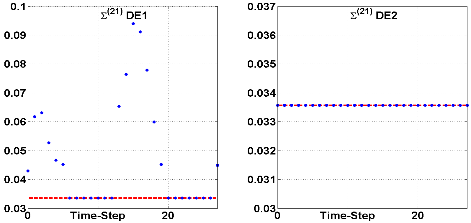
where vect⁡(M)\mathrm{vect}(M) is the vector formed by the diagonal entries of the matrix MM and ‖v‖1\|v\|_{1} is the 11-norm of vector vv. a1=750a_{1}=750 is the weight given to ϵ\epsilon in the cost function. This value of a1a_{1} gives the best trade-off between the following two objectives. The first objective is to minimize the first term in the cost function, where the 11-norm is used as a heuristic for finding diagonal gramians with many entries equal to ϵ\epsilon. We intend to truncate all the temporal and spatial state variables whose corresponding entries in the gramians are equal to ϵ\epsilon. The second objective is to minimize ϵ\epsilon since, by Corollary 1, ‖(G−Gr)‖<2​ϵ\|(G-G_{r})\|<2\epsilon. We get ϵ=0.034\epsilon=0.034, i.e., ‖(G−Gr)‖<2%​γ\|(G-G_{r})\|<2\%\gamma. Figure 2 shows the first and second diagonal entries of Σ(21)​(t)\Sigma^{(21)}(t), for 0≤t<280\leq t<28. The red dashed line corresponds to ϵ\epsilon. The dimension of x(21)x^{(21)} varies between 00 and 11 in GrG_{r} in contrast to 33 in GG, i.e., in GrG_{r}, the interconnection (2,1)(2,1) disappears at certain time-steps from the interconnection structure. As can be seen in Figure 3, between 1414 and 1818 temporal variables and between 2020 and 2525 spatial variables are truncated at each time-step. Clearly, truncation need not be uniform in time even if the dimensions of the states in the full order system are constants. We simulate GG and GrG_{r} for the same set of applied inputs and plot their responses in Figure 4. The inputs vary randomly between −10-10 and 1010 for the first 100100 time-steps and then are set equal to zero. As predicted by the error bound, the responses of GG and GrG_{r} are very close.

Refer to caption
Figure 2: First and second diagonal entries (DE) of Σ(21)​(t)\Sigma^{(21)}(t).
Refer to caption
Figure 3: Number and type of truncated state variables as function of time.
Refer to caption
Figure 4: Responses of the full order and reduced order systems for the same set of applied inputs.

7 Conclusion

This work applies BT for the model reduction of distributed LTV systems. The method provides a priori error bounds, preserves the interconnection structure, and allows for its simplification. While BT is only applicable to strongly stable systems, CFR extends the applicability of BT to strongly stabilizable and strongly detectable systems.

Acknowledgment

This work is supported by the National Science Foundation under Grant CMMI-1333785.

References

  • Abou Jaoude and Farhood (2015) Abou Jaoude, D., Farhood, M., 2015. Balanced truncation of linear systems interconnected over arbitrary graphs with communication latency, in: Proceedings of the 54th IEEE Conference on Decision and Control, Osaka, Japan. pp. 5346–5351.
  • Abou Jaoude and Farhood (2016) Abou Jaoude, D., Farhood, M., 2016. Coprime factors model reduction of spatially distributed LTV systems over arbitrary graphs. IEEE Transactions on Automatic Control doi:10.1109/TAC.2016.2638039.
  • Al-Taie and Werner (2016) Al-Taie, F., Werner, H., 2016. Structure-preserving model reduction for spatially interconnected systems with experimental validation on an actuated beam. International Journal of Control 89, 1248–1268.
  • Beck et al. (1996) Beck, C.L., Doyle, J., Glover, K., 1996. Model reduction of multidimensional and uncertain systems. IEEE Transactions on Automatic Control 41, 1466–1477.
  • Dullerud and DflAndrea (2004) Dullerud, G.E., DflAndrea, R., 2004. Distributed control of heterogeneous systems. IEEE Transactions on Automatic Control 49, 2113–2128.
  • Dullerud and Lall (1999) Dullerud, G.E., Lall, S., 1999. A new approach for analysis and synthesis of time-varying systems. IEEE Transactions on Automatic Control 44, 1486––1497.
  • Farhood (2012) Farhood, M., 2012. LPV control of nonstationary systems: A parameter-dependent Lyapunov approach. IEEE Transactions on Automatic Control 57, 212––218.
  • Farhood and Beck (2014) Farhood, M., Beck, C.L., 2014. On the balanced truncation and coprime factors reduction of Markovian jump linear systems. Systems and Control Letters 64, 96–106.
  • Farhood et al. (2015) Farhood, M., Di, Z., Dullerud, G.E., 2015. Distributed control of linear time-varying systems interconnected over arbitrary graphs. International Journal of Robust and Nonlinear Control 25, 179–206.
  • Farhood and Dullerud (2007) Farhood, M., Dullerud, G.E., 2007. Model reduction of nonstationary LPV systems. IEEE Transactions on Automatic Control 52, 181–196.
  • Hinrichsen and Pritchard (1990) Hinrichsen, D., Pritchard, A.J., 1990. An improved error estimate for reduced-order models of discrete-time systems. IEEE Transactions on Automatic Control 35, 317–320.
  • Kubrusly (2011) Kubrusly, C.S., 2011. The elements of operator theory. Second ed., Birkhauser, Basel.
  • Li and Paganini (2005) Li, L., Paganini, F., 2005. Structured coprime factor model reduction based on LMIs. Automatica 41, 145–151.
  • Lofberg (2004) Lofberg, J., 2004. YALMIP: A toolbox for modeling and optimization in MATLAB, in: Proceedings of the CACSD Conference, Taipei, Taiwan. pp. 284–289.
  • Sandberg and Murray (2009) Sandberg, H., Murray, R.M., 2009. Model reduction of interconnected linear systems. Optimal Control Applications and Methods 30, 225––245.
  • Sandberg and Rantzer (2004) Sandberg, H., Rantzer, A., 2004. Balanced truncation of linear time-varying systems. IEEE Transactions on Automatic Control 49, 217–229.
  • Sootla and Anderson (2016) Sootla, A., Anderson, J., 2016. On existence of solutions to structured Lyapunov inequalities, in: Proceedings of the American Control Conference, Boston, MA. pp. 7013–7018.
  • Toh et al. (1999) Toh, K.C., Todd, M.J., Tutuncu, R.H., 1999. SDPT3 — a Matlab software package for semidefinite programming. Optimization Methods and Software 11, 545–581.
  • Trnka et al. (2013) Trnka, P., Sturk, C., Sandberg, H., Havlena, V., Rehor, J., 2013. Structured model order reduction of parallel models in feedback. IEEE Transactions on Control Systems Technology 21, 739–752.