Stochastic spatial models in ecology: a statistical physics approach
Abstract
Ecosystems display a complex spatial organization. Ecologists have long tried to characterize them by looking at how different measures of biodiversity change across spatial scales. Ecological neutral theory has provided simple predictions accounting for general empirical patterns in communities of competing species. However, while neutral theory in well-mixed ecosystems is mathematically well understood, spatial models still present several open problems, limiting the quantitative understanding of spatial biodiversity. In this review, we discuss the state of the art in spatial neutral theory. We emphasize the connection between spatial ecological models and the physics of non-equilibrium phase transitions and how concepts developed in statistical physics translate in population dynamics, and vice versa. We focus on non-trivial scaling laws arising at the critical dimension of spatial neutral models, and their relevance for biological populations inhabiting two-dimensional environments. We conclude by discussing models incorporating non-neutral effects in the form of spatial and temporal disorder, and analyze how their predictions deviate from those of purely neutral theories.
I Introduction
Community ecology aims at shedding light on how competing species assemble and coexist in their habitats [1]. This has proven to be a formidable challenge. A main reason is that ecological dynamics span a wide range of spatial and temporal scales, from those typical of individuals to those characterizing large populations or communities. Ecologists have empirically characterized biodiversity at the different spatial scales; for example, counting the average number of species hosted in a given area – species area relationship (SAR) [2, 3]–, or the distribution of their abundances – species abundance distribution (SAD) [4, 5]. Often, the ecological forces determining these patterns act at a given spatio-temporal scale but can affect others as well. The inverse problem, i.e. linking observed patterns with the causes originating them at different scales, is arguably the central problem in ecology [6].
This kind of problem sounds familiar to experts in statistical physics, where large-scale emergent behavior results from interactions among simple local units. Tools of statistical physics are indeed very useful to make progress on the aforementioned crucial issues in ecology. In particular, a natural approach to such complex problems is to radically simplify them. To this aim, we consider ecosystems made up of competing non-motile species, such as trees, or having a motility range much smaller than the typical linear size of the population, such as communities of microorganisms. Further possible simplifications are that all emergent phenomena originate at the single-individual scale and, more drastically, that differences among individuals, possibly belonging to different species, can be neglected. These assumptions constitute the basis of the ecological neutral theory proposed by Hubbell [7].
Ecological neutral theory [7] was built upon theoretical ideas of Kimura’s neutral theory of population genetics [8]. Both theories underscore the role of stochastic demographic fluctuations in determining the fate of populations and completely neglect deterministic effects stemming from fitness differences. The assumption of ecological neutrality has elicited heated controversies, as it hinted that classical ecological concepts, such as niches, might play a marginal role in structuring communities of competing species. Despite these contentions, neutral theory had a considerable impact on ecological thinking, owing to its ability to quantitatively predict non-trivial patterns of biodiversity with simple models characterized by very few adjustable parameters [9, 10, 11].
Spatially implicit neutral models describe well-mixed communities of individuals subject to immigration from a larger reservoir of species where diversity is maintained via speciation. They can be solved analytically [12, 13, 14, 15, 16], yielding analytical expressions for the SAD. Beside the mathematical appeal, these exact solutions have been extremely helpful for fitting empirical data and therefore testing neutral theory or, at least, promote it as a null-model [17]. For more exhaustive surveys of ecological neutral theory, we refer the reader to Hubbell’s book [7] and the reviews [9, 10, 11].
The focus of this review is on spatially-explicit neutral and near-neutral population models. Explicitly describing space is crucial to address the fundamental ecological questions sketched at the beginning of the introduction. However, spatially-explicit models – that are often variants of familiar models in non-equilibrium statistical physics [18] – are still poorly understood, especially if compared with their well-mixed counterparts [19]. One of the most studied neutral model is the voter model with speciation, or multi-species voter model [20, 21, 22], which generalizes the more common two-species voter model [23]. The stepping-stone model [24, 25, 26, 27] and the contact process [23, 28, 29] are other examples of spatial models that have been studied in both the physics and population biology literature. We shall discuss how these analogies can be used to advance our understanding of spatial ecology and the main open problems. This review heavily relies on extensive numerical computations of lattice models based on previous works by the authors. This might have biased the choice of some topics and we apologize if some relevant works are not properly discussed.
The review is organized as follows. In Sect. II we introduce the multispecies voter model on a lattice and its dual representation in terms of coalescing random walkers. We then discuss its predictions of macroecological patterns: the SAR, and the SAD. For the latter, we compare two recent analytical approaches [30, 31, 32] with novel computational results. We mainly discuss the two-dimensional case due to its ecological relevance, but also briefly present the one-dimensional case for comparison. We conclude the section by presenting new results on an important dynamical property: the distribution of species persistence-times. In Sect. III we discuss other neutral models, where, at variance with the voter model, lattice sites are not necessarily occupied by exactly one individual at all times. In particular, we consider the stepping stone model, where each lattice site hosts a local community of individuals. This generalization is relevant for modeling microorganisms and their macroecological patterns. We then consider a multispecies variant of the contact process, where lattice sites can be either empty of occupied by single individual. In Section IV we introduce non-neutral effects on a simplified two-species competition model, where adjusting a single parameter one can tune the departure from neutrality, here modeled as a specific habitat preference. Physically, this habitat preference can be thought as a form of quenched disorder. We discuss how this disorder generically favors species coexistence using the language of statistical mechanics, and also discuss other forms of disorder such as temporal heterogeneity. Finally, Sect. V is devoted to perspectives and conclusions.
II Voter Model with speciation
II.1 Description of the model
A paradigmatic example of spatial neutral model is the voter model with speciation, [20], which is is a multispecies generalization of the voter model [23]. The latter is a widely studied model that has been applied in diverse contexts, from population genetics to spatial conflicts [33], spreading of epidemic diseases [34], opinion dynamics [35] and linguistics [36].
The voter model with speciation is defined on a lattice, where each site hosts one individual belonging to some species. At each discrete time step, a lattice site is chosen at random and the residing individual is removed (death event). Then, as illustrated Fig. 1, the dead individual is replaced:
- •
- •
With complementary probability , by a new individual of an existing species (reproduction event). In this case, the newborn belongs to the same species of a parent individual chosen at random in the neighborhood of the vacant site. In the simplest case, the nearest-neighbors (NN) are chosen with uniform probability. More generally, the parent individual is selected according to a probability distribution (the dispersal kernel) over the neighbors within a distance .

Most of this section will be devoted to the ecologically relevant case where the system is a two-dimensional () square lattice, although we will briefly present some results in for comparison.
II.2 Duality
The voter model with speciation is dual to a system of coalescing random walkers with an annihilation rate [38, 39, 20]. In this context, “duality” means that each trajectory of one system can be mapped in one of the other system having equal probability [38]. The dual process is constructed as follows. We start by placing on each lattice site a random walker. The dynamic of the dual process proceeds backward in time. At each discrete (backward) time step, with probability , a randomly chosen walker is moved to a new site, where the dispersal kernel here plays the role of the distribution of possible displacements. If the site is occupied, the two walkers coalesce, i.e. one of the two is removed keeping trace of the coalescing partner. With complementary probability a randomly chosen random walker is annihilated, i.e. removed from the system. This event corresponds to a speciation event in the forward dynamics. The whole tree of coalescing random walkers, before annihilation, represents the entire genealogical tree of a species up to the speciation event that originated it.
The standard forward in time evolution of the voter-model with speciation and its dual dynamics are sketched, for the one-dimensional case, in Fig. 2a and 2b, respectively.

Duality is a very useful property to understand the physics of the voter model. For example, it immediately stems from duality that the limit is fundamentally different in and . As a matter of fact, in the random walk is recurrent, meaning that the probability of two randomly chosen individuals to belong to the same species approaches one as . In other words, in the absence of speciation, one has monodominance of one species in the long term. The same property does not hold in , where random walkers are not recurrent and, in an infinite system, multiple species coexist on the long term even in the limit . Interestingly, the ecologically most relevant case, , is the critical dimension of this model. We shall see that this fact is a source of non-trivial behaviors of ecologically relevant quantities.
Duality is also an extremely powerful tool for computational analyses [21, 22]. If one is interested in the static, long-term, properties of the voter model with speciation, it is numerically much more efficient to simulate the dual dynamics than the forward one. In a dual simulation, after all walkers coalesced or were annihilated, species can be assigned to the start site of each walker, obtaining a stationary configuration of the voter model. Beside computational speed, this approach has also the advantage of eliminating finite-size effects induced by the boundary conditions, as the coalescing random walkers can be simulated in a virtually infinite system. For illustrative purposes, in Fig. 2c and 2d we show two configurations of the voter model obtained with the dual dynamics for two different dispersal kernels.
II.3 diversity
The first ecological pattern we consider is the -diversity, which is a measure of how the species composition in an ecosystem varies with the distance. We define the -diversity as the probability , that two randomly chosen individuals at a distance are conspecific, i.e. belong to the same species. We remark that, although this is the natural definition in this context, other definitions have been used in the ecological literature [40]. Mathematically, can be expressed in terms of the two-point correlation function , where denotes the number of individuals of species at location
| (1) |
where the sums extend over all species in the ecosystem [11]. Eq. (1) can be used to estimate the -diversity as the ratio between the couples of conspecific over the total number of couples in a sample.
Let us now study the evolution equation of for the voter model with speciation and NN dispersal. Although we shall focus on the case, it is useful to present the general calculation in dimensions. Following [41, 42, 11] we write
| (2) | |||||
The first term in the r.h.s. of Eq. (2) represents the fact that does not change if two generic individuals at distance are not removed in a given time step and therefore survive. The second term represents the events in which one of the two individuals dies (with prob. ), no speciation occurs (with prob. ) and the dead individual is replaced by a conspecific from the neighbor sites. Taking the continuous limit with the lattice spacing , the speciation probability , and a finite value of , one obtains at stationarity the differential equation
| (3) |
where is the dimensional Dirac delta, and because of isotropy the -diversity is now function of only. The solution of Eq.(3) is [11]
| (4) |
where is the modified Bessel function of the second kind of order and the constant is fixed by the condition . We recall that Eq. (4) is a continuous expression, valid for distances much larger than the lattice spacing [41]. Although we derived Eq. (4) for NN dispersal, the same results hold for a general dispersal kernel for distances larger than the kernel range, provided that the kernel range is finite.
For , Eq. (4) implies that , which is characterized by a slow logarithmic decay, , up to distances of order , followed by a faster, exponential falloff. Remarkably, the -diversity empirically measured in several tropical forests in Central and South America is consistent with a logarithmic decay for large distances [43]. We remark that this logarithmic decay is the signature that is the critical dimension for the voter model. In contrast, in , Eq. (4) becomes . We mention for later convenience that, in with NN dispersal, Eq. (2) can be solved without using the continuous approximation, giving [42]
| (5) |
where for .
Although the -diversity decays exponentially on scales both in and , there are important differences. Because is the critical dimension, a large biodiversity (i.e. a large average number of species) can be sustained by very low values of the speciation rate . This implies that in there are many species living on scales much smaller than , where the correlations decay logarithmically. Conversely, in to maintain biodiversity one needs a large value of , so that is the only characteristic scale and there is no additional structure on scales smaller than . This crucial point will be further elucidated in the rest of the section, where we will discuss other observables in (subsections II.4 and II.5) and compare them with their counterparts.
II.4 Species-Area Relationships
We now focus on the SAR, defined as the average number of species, of a given taxonomic level occupying a given area of size . SARs are widely studied as a measure of spatial biodiversity and quantify how larger habitats support more species than smaller ones [3]. Empirical measures of SARs at multiple scales often reveal three different regimes [2, 3, 7]. At small areas, the number of species increases rather steeply, nearly linearly, with the sampled areas. A similar steep increase is observed at very large, continental scales. Instead, at intermediate scales, a slower, sublinear growth is often found. Such a growth is well approximated by a power law , , over a wide range of taxa [44], though a logarithmic behavior has also been proposed. An extensive meta-study by Drakare et al. [45] reconsidered a large body of SAR studies from the literature, revealing that the power law provides a better fit in about half of the cases. This study also observed that the exponent correlates positively with the body size of the considered group of species, so that small microorganisms typically display very shallow SAR curves as compared with larger organisms (see also [46] and Sect. III.1).
Simulations of the (dual) voter model with speciation yields SARs qualitatively similar to those obtained from field data, see Fig. 3a. In the voter model, the steep initial regime is mostly determined by the dispersal range . For areas significantly larger than , a sublinear growth is observed (see Fig. 3b. In this regime, the growth becomes progressively more shallow as the speciation rate is decreased. For larger scales, the logarithmic slope of the SAR curves become steeper again. The area at which this final crossover occurs increases as is decreased.
An interesting question is whether the sublinear growth regime in the voter model can be characterized by a power-law and, in this case, what is the value of the exponent as a function of . To address this question, we begin by reviewing a classic estimate of by Durrett and Levin [20] relying on duality (see Sect. II.2). The speciation rate sets a time scale which also corresponds to a characteristic length scale because of the diffusive behavior of random walkers in the dual model. Walkers with an initial separation much larger than are likely to be annihilated before coalescence occurs. This observation alone explains the linear scaling of for areas . At these scales, species are uncorrelated, as can also be inferred from the analysis of the -diversity in the previous section. For a system of coalescing random walkers in , the density of occupied sites decays asymptotically as [47, 48]
| (6) |

The characteristic logarithmic coarsening of clusters observed in the voter model without speciation can be related to the logarithm appearing in Eq. (6) [49]. Assuming , the annihilation rate at time in an area can be approximated as the annihilation rate per walker times the number of walkers in the absence of annihilations . Integrating over time, we find that the total number of annihilations, i.e. the total number of species, is [39]
| (7) | |||||
where is the time at which the asymptotic expression (6) starts to be valid. The upper temporal cut-off is set to (with ) because the number of killing events occurring after a time is bounded by the number of walkers in the system, which is [39]. Finally, combining Eq. (7), the fact that and matching a power law behavior in the range of scales from to , one finds [20]
| (8) |
Also in this case, the logarithmic dependence of the exponent on derives from the fact that is the critical dimension for the voter model.
More recent results disputed the validity of Eq. (8). Scaling arguments hinted that should approach a finite value in the limit of vanishing (see [42] and Sec. II.5.1), while numerical simulations suggested a power law dependence, [21]. Finally, further numerical simulations, based on the dual representation of the voter model with speciation (see Sect. II.2) and spanning a very wide range of speciation rates from to confirmed the logarithmic behavior predicted by Eq. (8) [22]. The exponents measured in such simulations, shown in Fig. 3c, are well fitted by a phenomenological expression of the form
| (9) |
which is consistent with Eq. (8) up to order , see also Fig. 3d. However, fitted values of the prefactors and are not consistent with Eq. (8). This discrepancy is probably due to pre-asymptotic effects as well as to the approximation of assuming a power-law range between and .
Let us briefly discuss the role of the dispersal kernel. As illustrated in Figs. 3c and 3d, a comparison between NN dispersal and a square dispersal kernel of range demonstrates that the exponent depends to some extent on the dispersal kernel. However, numerical evidence [21, 22] suggests that when the dispersal kernel range is large enough (approximately ) the exponents are very weakly dependent on . Moreover, SARs obtained with different values of can be rescaled onto a universal function of and via the transformation with a fitted value of . To the best of our knowledge, a formal derivation of this scaling law and of the exponent is currently an open problem.
The non-trivial area dependence of the SAR results is a special feature of the critical dimension . To highlight this point, we now discuss the case as comparison. This case is also relevant to describe quasi one-dimensional ecosystems, such as river basins [50]. For simplicity, we limit ourselves to the case of NN dispersal.
To the best of our knowledge, also in , an exact expression for the average number of species, , in a segment of length is unknown. Nevertheless, it is possible to provide a lower and upper bound for . In , the density of walkers behaves as , to be contrasted with eq. (6) valid in the case. Dimensional arguments then suggest that the average number of species must a function of only, i.e. . Computational results (Fig. 4a and inset) support well this simple argument. As shown in the figure, the non-trivial power-law regime characteristic of SARs is absent in . Indeed, the function is linear for large arguments, with a coefficient around and it is nearly constant for .

We can derive an upper bound to using that, in , individuals are organized in segments of conspecific individuals, so that , with the equality holding if no species is present in more than one segment. We compute from the probability , with given by Eq. (5), that two sites and are occupied by conspecific individuals [51]
| (10) | |||||
which for can be approximated as .
II.5 Species-Abundance Distributions
We now discuss Species-Abundance Distributions (SADs), , that measure the relative abundance of species in a given area . More precisely, denoting the total number of species sampled in an area , each composed by () individuals, is the probability that a randomly picked species has an abundance between and . While the expression of for well-mixed neutral models is known [14], computing it for spatially explicit models, such as the voter model with speciation, has proven to be a rather hard problem. We first discuss in section II.5.1 an approach based on standard finite-size scaling, and underline its limitations. In Sec. II.5.2, we discuss how this approach can be generalized at the critical dimension, present numerical results, and discuss a recent attempt to compute exploiting duality. Although we focus ond comparing the scaling theory with results from the voter model with speciation, we remark that the theoretical approach presented in this section is more general and can be applied to a vast class of models at the critical dimension.
II.5.1 Power-law scaling relation
In the voter model with speciation, the SAD is not only a function of the system size , but also of the speciation rate . Although we are mainly interested in , it is instructive to consider the general case in which , where is the linear size of the sample. Following [42, 11], we assume a standard scaling form for the SAD
| (12) |
where the exponents and remain unspecified for the time being, whereas the exponent stems from the diffusive nature of neutral models . Note that in models with long-range, non-diffusive dispersal [52] the scaling form might differ. Equation (12) describes a power-law dependence of on , holding up to a scale determined by the scaling function , that depends on dimensionless combinations of the population size , the speciation rate , and the system size . To the best of our knowledge, there is no available analytical prediction for the exponent . The exponent can be estimated in the dual formulation of the voter model with speciation, where the population size is the number of coalescences that occur before an annihilation (see Sec. II.2). This implies that is the same exponent characterizing the temporal decay of the density of coalescing random walkers, . However, decays as for and in , see eq. (6) and [53, 48]. Consequently, one should expect the power-law scaling of Eq. (12) to hold in and , but not at the critical dimension , where logarithmic corrections should appear.
II.5.2 Generalized scaling relation
In order to allow for logarithmic corrections, Zillio et al. [30] proposed the generalized scaling relation
| (13) |
The dependence on was omitted as the above scaling law was applied to observational data for which the speciation rate is unknown and assumed to be fixed. The key aspect of Eq. (13) is that and , are general functions and not necessarily power-laws as in conventional scaling, allowing for the possibility to include logarithms or other functional dependencies. The scaling function is still assumed to be a power law
| (14) |
for small values of , where is an exponent to be determined. Thus, also Eq. (13) postulates a power-law dependence on , but with a more general cut-off for large areas. After specifying the functions and , Eq. 13 can be tested by plotting versus for a set of different areas and assessing the quality of the data collapse onto a single curve, .
To determine the functions and , we impose that has to be normalized, , and that its average value has to be . Substituting the scaling form (14) into these two equations, it is possible to derive conditions that the functions and must obey, depending on the value of . In particular, the case is marginal and needs to be treated with care (other values are analyzed in the Appendix). Approaching such a limit as with , Eq.(14) becomes
| (15) |
up to first order in . At the same order in , the two conditions for become and , respectively, from which we finally obtain
| (16) |
up to first order in . Notice that both functions and include logarithmic corrections. By means of a similar calculation, one can estimate the -th moment , and verify that all the moment ratios scale in the same way, up to a multiplicative constant
| (17) |
revealing a highly anomalous scaling.
Zillio et al. [30], showed that this scaling form provides a much better collapse of empirical data from the Barro Colorado tropical forest than a power-law scaling relation such as Eq. (12). This supports the idea that is close to its marginal value in tropical forests.

We tested computationally whether Eqs. (13) and (16) provide a good collapse of SADs obtained from the voter model with speciation and whether the relationship between the moments, Eq.(17), holds. In simulations, an additional parameter is the speciation rate . As discussed above, appears in scaling relationships via the dimensionless combination , that in equals . Thus, although Eqs. (13) and (16) do not include speciation explicitly, we expect these relationships to hold if is kept constant. We therefore performed computational analyses fixing , although the conclusions are robust against this choice. Results are summarized in Figure 5 which shows plots of the SAD, for systems with different linear size, and different speciation rates (with ). Observe in Fig. 5a that the smaller the size (or the larger the speciation rate) the smaller the maximal abundance. Figure 5b show the data collapse as given by Eqs. (13) and (16), where is the average number of individuals measured in each area and is a free parameter that we fitted obtaining and a remarkable collapse of the different curves. The small value of , is consistent with the assumed small deviation from . A similar collapse for leads to an even smaller value (not shown). We verified that either removing all logarithmic corrections (thus plotting results as a function of ) or simply fixing in Eq. (13) and (16) leads to less convincing collapses, as shown in Fig. 5c and 5d, respectively. Clearly, these deviations can pass unnoticed in the presence of statistical fluctuations. Probably, this is the reason why in [54] a simple scaling law was claimed to hold for the voter model with speciation. Finally, we also verified that moment ratios scale as , as predicted by Eq.(17) and illustrated in Fig.6.

In summary, a non-standard scaling form, including logarithmic corrections, provides an excellent collapse both for empirical data and for numerical simulations of the voter model. We remark that the scaling theory is phenomenological, and the small parameter controlling the importance of logarithmic corrections is, at this level, a non-universal free parameter. These results are in sharp contrast with the one-dimensional case, where logarithmic corrections are not expected. Indeed, Fig. (7) shows that the naive scaling form vs. (derived in Appendix A for the case ) yields a perfect collapse for SADs in one-dimensional systems.
It is interesting to remark that the data collapsed in [30] were obtained from tropical forests of different areas . It is reasonable to assume that the speciation rate do not vary much among these forests. Therefore, the product is not fixed, as in our computational analyses. A possible explanation is that, although the collapse achieved in this way is not perfect, the deviations from perfect scaling are too small to be appreciated in observational data due to the limited sample size. We have verified in simulations (not shown) that keeping constant (rather than constant) small deviations from perfect collapse are observed.

We conclude this section mentioning that a heuristic expression for the SAD has been recently derived for the voter model with speciation following a completely different approach [32, 31]. Let us define as the distribution of the number of individual of a given species at time . If we approximate as a continuous quantity, we can heuristically write a Fokker-Planck equation for the evolution of
| (18) |
where the first term in the right hand side is the negative drift due to speciation, and the second is the fluctuation in population size, where is the average number of interfaces of a species of size . The crucial underlying approximation is to neglect fluctuations of , which is appropriate if the distribution of the number of interfaces at fixed value of is a very peaked function. In this simple framework, all the dependence on the spatial dimension of the voter model is recap into the function . The steady-state solution of Eq. (18) is
| (19) |
From duality considerations [32, 31], the average number of interfaces must scale in as where is a non-universal constant. Notice how the expression of includes familiar logarithmic terms and that the constant plays the role of the exponent in the scaling theory. Substituting this expression into Eq. (19) leads to an explicit expression for the SAD, which obeys a scaling law with logarithmic corrections similar to Eq. (16), though not identical. A more detailed comparison between this result and the previous scaling form is an interesting issue, but beyond the scope of this review.
II.6 Species persistence-times
So far, we have considered neutral predictions of static ecological observables. However, neutral theory can also be used to predict time-dependent properties. A chief example is the distribution of survival times. The survival time (also called ”persistence time”) within a geographic region is defined as the time occurring between the speciation event originating a given species and its local extinction [15]. Recent empirical work on north-american birds and herbaceous plants revealed that the probability of observing a persistence time decays as as power laws and respectively, with area-dependent exponential cut-offs [55, 56].
In the voter model with speciation, the survival probability as a function of time can be computed analytically. Also in this case, the calculation relies on duality [47, 48, 57]. In and in the limit of vanishing one obtains
| (20) |
while standard power-law scaling is expected in 1D. For non-negligible values of , these scaling forms are cut-off by a -dependent exponential factor in either dimension. Also in this case, diffusive scaling relates the characteristic time scale with a length scale via . This explains the aforementioned area-dependent cut-offs observed in empirical data [55].

Species persistence times in simulations of the voter model with speciation are shown in Fig. 8a. Panels (b) and (c) show compensated plots of the simulation results. The simulations support the prediction of eq. (20) (panel b), and also illustrate that a power law with an exponent close to ( in this case) provides a good approximation of the scaling predicted by Eq. (20) in a broad range of scales (panel c), consistently with the empirical findings in [55, 56].
III Other neutral models
In the voter model with speciation, the habitat is saturated and each site is always occupied by an individual. In this section, we study neutral spatial models where the number of individuals that can inhabit a site is varied. We consider three variants: the stepping-stone model with speciation, where each site can host many individuals but the landscape remains saturated; the contact process with speciation, where occupancy is limited to a maximum of one individual per site, but sites can also be empty; and the O’Dwyer-Green model, where occupancy is unbounded.
III.1 Stepping-Stone Model with speciation
In the voter model, each lattice site hosts a single individual. This assumption is appropriate for big sessile species, such as trees, where each individual occupies a well-defined area and exploits its local resources. On the other side of the spectrum, microorganisms, such as small eukaryotes or bacteria, are often present in very large numbers on tiny spatial scales, where all individuals share the same resources. For these species, it is more appropriate to think of the habitat as subdivided into small patches, connected by migration and each hosting a large number of individuals directly competing with each other [58]. To model such ecological cases, in this section we consider the stepping-stone model [25, 26] with speciation, which generalizes the voter model with speciation to the case in which each site hosts a fixed number of individuals.
Similar to the voter model with speciation, at each time step an individual is randomly chosen and killed. With probability , it is replaced by an individual of a novel species. With complementary probability , a reproduction event occurs. The parent of the new individual is selected with probability among the surviving individuals present at the same site, and with probability among the individuals in a randomly chosen neighboring patch (according to a probability distribution on the neighbors , similar to the case of the voter model). The particular case of reduces to the voter model with speciation up to a time rescaling . Like the voter model, the stepping-stone model admits a dual representation in terms of coalescing random walkers with annihilation, which can be exploited for efficient numerical simulations. The main difference with respect to the dual of the voter model is that, in the dual stepping-stone model, at each step a random walker can either move to another site or stay in the site of origin. Coalescence can happen in both circumstances, corresponding to reproduction of an individual from neighboring sites or from the same site. For full details on the implementation we refer to [27].
As revealed by numerical simulations of the stepping-stone model based on the dual representation, SARs are qualitatively similar to those of the voter model, although the exponents are, in general, smaller than in the voter model [27]. In particular, the exponent depends not only on , but also on the combination of parameters , which determines the regimes of the model. For , each local site is likely to contain only one species. In this limit, each site behaves as one individual up to a time rescaling, so that one should expect the same exponents as in the voter model with speciation. In the opposite limit , there is a large diversity of species at each site. An analytical argument suggests that, in this latter limit, the exponent should be a factor two smaller than in the former limit [27]. Let us study the limit in the dual representation. Since random walkers in the same site have a low probability of coalescence, they will wander for a long time before coalescing. Therefore, we can assume that, asymptotically, they will behave as in the well-mixed case. This implies that their density in an area smaller or equal than approximately decays according to the mean-field formula
| (21) |
Observe that in this case the characteristic length is , as random walks diffuse with probability at each time step. Proceeding as in Eq. (7), the average number of species in an area can be estimated as
| (22) |
To compute , we also need an estimate for , that in this case is not trivially equal to one. As the population is assumed to be well-mixed in an area equal to or smaller, the composition of a single site can be thought as a sample of individuals from this well-mixed population. The probability distribution of the abundance in such a sample is given by Ewens’ sampling formula [59]. Substituting its expression yields
| (23) |
Combining Eqs. (22) and (23) and assuming a power law in the range from to , we find an exponent
| (24) |
which, to the leading order, is a factor smaller than the corresponding estimate for the voter model (8). The decrease of the exponent with the combination of parameters is confirmed in numerical simulation, see Fig. 9, although the asymptotic reduction is less than the factor two predicted by the approximate estimate of eq. (24).

Summarizing, the stepping-stone model at large local community size yields smaller values of the species-area exponent than the voter model [27]. This fact is consistent with the ecological observation that microbial communities, characterized by very large local community sizes, typically display very shallow species-area relations, and that in general there seems to be a positive correlation between the exponent and the body size of a taxonomic group [46]. In the stepping-stone model, a decrease in the SAR exponent is observed in the regime where each site hosts a large number of species and therefore provides a buffer for biodiversity [27]. This interpretation is also consistent with the “cosmopolitan” nature of many microbial species, i.e. the fact that relatively small communities of microbes host a biological diversity comparable with that observed in the whole planet [60, 58]. This feature has sometimes been explained invoking the fact that microbes have the possibility of long-range dispersal [60]. However, numerical simulations show that, in the voter-model with speciation, long-range dispersal leads to steeper, rather than shallower SARs [52].
III.2 Contact Process with speciation
In the voter model, every dead individual is instantly replaced by a newborn, leading to a constantly saturated environment. The implicit underlying assumption is that the birth rate is infinite, so that death events are the rate-limiting steps. Such assumption constitutes a good approximation in resource-rich ecosystems. In less rich ecosystems, where the birth rate is finite, the environment is not always saturated and empty gaps can exist [61].
To explore this latter case, we study here the contact process with speciation, which is the multi-species variant of the well-known contact process [62, 38, 18, 28, 29]. As usual, we consider the model on a square lattice. Sites of the lattice can be occupied by individuals belonging to different species or empty. The model is defined in continuous time; each individual dies at a rate and reproduces at a rate . In case of a death, the site is simply left vacant. A reproduction event is considered successful only if the individual has at least one vacant neighboring site. In such a case, one of the vacant neighboring sites is chosen at random. With probability , the site is occupied by an individual of a new species (speciation event); with complementary probability, , the newborn is of the same species as the parent.
As in the standard contact process [62, 38], the parameter determining the asymptotic density of occupied sites is the dimensionless birth-to-death ratio . For the absorbing state in which all sites are empty is stable. A non-equilibrium phase transition at separates this region from a stable active phase () characterized by a non-vanishing value of that depends on [28, 29]. For one has and the model is equivalent to the voter model with speciation [18].
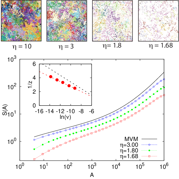
The CP is a self-dual model. Therefore, duality cannot be exploited in numerical simulations as in the case of the voter model. Forward simulations show that the SAR and the corresponding exponents are remarkably similar to the voter model with speciation even at small values of , corresponding to very fragmented ecosystems as shown in Fig. 10. For values of very close to (but within the active phase) and small values of , SAR exponents tend to be smaller than in the voter model, see inset of Fig. 10.
In principle, in a very fragmented ecosystem it would not make sense to sample empty areas, or areas with very few individuals. With this idea in mind, an alternative to the standard definition of SAR used so far is to weigh the sample of a given area with its number of individuals, i.e. of occupied sites. Adopting this definition one finds qualitatively different SARs for small values of [27]. In particular, these SARs do not seem to be characterized by a clear power-law range. We refer the reader to Ref. [27] for a broader discussion of this issue.
III.3 O’Dwyer-Green model
We have seen that finding exact results for neutral spatial models constitutes a formidable problem, and even in the simple case of the voter model only asymptotic results are known.
To make progress in this direction, O’Dwyer and Green proposed a spatial neutral model in which individuals do not compete, i.e. the site occupancy is not bounded [63]. In their model, each individual can reproduce at a rate , giving rise to a newborn located according to a dispersal distribution, die at a rate , or speciate at a rate , giving rise to a newborn of a new species. The model was studied at the critical point . The lack of interaction considerably simplifies the mathematical treatment: the model can be mapped into a field theory from which the authors of [63] obtained an analytical expression for the species-area law and the dependence of on . In particular, the solution was derived by writing an equation for the distribution of a generic species, which was solved by imposing detailed balance. However, Grilli and coworkers [64] pointed out a flaw in this procedure. In this model all species are transient, as the birth rate of each species is always smaller than the death rate because of speciation. This implies that all species eventually go extinct, so that the detailed balance (i.e. equilibrium) assumption is not valid.
An often overlooked aspect of the O’Dwyer and Green model is the lack of a carrying capacity. Although well-mixed neutral models commonly do not have a carrying capacity (beside that of the entire ecosystem), a local carrying capacity, i.e. a maximum occupancy of each lattice site, is a standard ingredient in spatial neutral theory, shared by all models we discussed so far. In the O’Dwyer and Green model, since the dynamics of the entire ecosystem is a critical branching process, the population at each site undergoes huge fluctuations. This fact implies as a drawback that numerically simulating the steady-state of the model and sampling its configurations is extremely difficult. While the authors of [64] clearly pointed out that the detailed balance solution leads to several inconsistencies and is therefore not valid, to the best of our knowledge there have been no attempt of comparing this solution with numerical simulations to see if detailed balance can provide a reasonable approximation of the dynamics in some particular regimes or limits.
Currently, the research of spatial neutral models that can be solved analytically is still open [65]. In this direction, although this review focuses on lattice models, we mention a recent phenomenological attempt based on a spatial Fokker-Planck equation where both space and population sizes are continuous variables [66].
IV Near-neutral models
In the previous sections, we focused on neutral ecological models. However, in real ecosystems the neutral assumption is (at best) a crude approximation. It is thus interesting to examine some of the main effects of non-neutral forces, also because many biodiversity patterns that are well predicted by neutral models are also found in richer, non-neutral models [67, 68, 69]. A main difficulty in comparing neutral and non-neutral models is the large number of possible ecological effects (and corresponding parameters) that typically enter the latter. In this section, with the aim of understanding basic non-neutral effects in a simple setting, we present a minimal model introduced in [70], where one can continuously move from a neutral to a non-neutral scenario by varying a single parameter, tuning the amount of spatial disorder. We then discuss generalizations to other types of spatio-temporal disorder.
IV.1 Habitat-preference model
We consider a variant of the voter model where different sites are preferred habitats for each one of the competing species. For the sake of simplicity, we limit ourselves to the case of two species and with and individuals, respectively. We assume habitat saturation, so that the total population is where the system is a square lattice of size with periodic boundary conditions. Individuals of type and can also migrate to the system from an infinite reservoir where they are equally represented. Each lattice site can be of type or , i.e. being a preferred habitat for colonization by species or , respectively. After colonization, mortality and dispersal do not depend on being on a preference site. Ecologically, this means that the fitness advantage belongs to the seeds and not to the individuals themselves (see [71] for a different choice). The vs character of each site is chosen randomly at the beginning and it remains fixed over time – quenched disorder. To maintain the model globally symmetric, we assume equal proportions of and sites and that intensity of the two biases ( favoring and favoring ) are identical. The dynamics proceeds as follows. At each discrete time step, a lattice site is randomly chosen with uniform probability and the residing individual is killed. The individual is replaced either by an immigrant from the reservoir (with probability ) or by an offspring of an individual residing in one of the four neighboring sites (with probability ). In both cases, the colonization probability is biased by an additional factor for the individuals that have preference for the empty site. In formulas, the probability of colonization of a site by an individual () having (not having) preference for that site is
| (25) |
respectively, where () denotes the number of individuals of species () in the neighborhood of the considered site. Similar models have been proposed also in the context of heterogeneous catalysis [72] and social dynamics [73]. For and , the standard (neutral) voter model with two species is recovered. For but , it corresponds to the noisy voter model [74, 75].
Also in this model, the results can depend on the choice of the dispersal kernel . Here we focus on the NN dispersal and global dispersal (GD), i.e. a mean-field version of (25). The GD case can be thought as a variant of the two islands model [76] of population genetics, where each island host individuals and is favorable to one of the two species. In the mean-field version, the state of the system is univocally determined by the numbers of individuals and residing on their island of preference. The numbers of individuals outside their island of preference are and . The dynamics is then fully specified by the probabilities per elementary steps that (with and ) increases or decreases by a unit:
| (26) |
where and are given by eqs. (25) with and replaced by and , respectively.
IV.2 Extinction times
In the absence of immigration () and for finite populations , persistent coexistence of the two species is not possible: demographic stochasticity eventually drives one of the species to extinction (the absorbing state) with the fixation (in the jargon of population genetics) of the other species. In this case, information on the system can be obtained by studying the dynamics toward extinction [71]. Of particular interest is the average extinction time, , and its dependence on system properties, such as the deviation from neutrality and the population size.
In the neutral case (), as discussed, the system recovers the voter model with NN dispersal and the Moran model [37] in the version with global dispersal. In this limit, the extinction time is set by the population size. In particular, for large we have for NN-dispersal [77] and for global dispersal [37, 78]. To inquire the effect of habitat preferences we performed simulations of the model (25) with an initial condition until the extinction of one of the two species.

Figure 11 shows the average extinction time, measured in generations, i.e. elementary steps of eqs. (25), as a function of the population size for different values of . For we observe the behavior expected in the neutral case. Habitat preference () leads to a dramatic increase of the average extinction time, which becomes exponential in
| (27) |
for large enough . The dependence of the constant on , shown in the inset, is well-fitted by a power-law with exponent . The mean-field version of the model presents similar qualitative features with the only difference that for and with some differences in the dependence of , as shown in [70].
The exponential dependence of the average extinction times on indicates that habitat preference has a stabilizing impact on the population dynamics. Indeed, when is large enough, the two species coexist on any realistic time scale. The stabilizing effect of habitat preference reflects also in the probability of fixation , i.e. the probability that a species, say , gets fixated when initially present as a fraction of the population. In the neutral case, standard computation [78] shows that . As shown in [70], when is increased, develops a much steeper dependence on and quickly reaches values even for small , provided that is large enough. In other words, the stabilization due to habitat preference tends to compensate any initial disproportion between the population of the two species.
IV.3 Coexistence
In the presence of immigration (), a locally extinct species can recolonize, leading to a dynamical coexistence between the two species. However, if the typical recolonization time is large compared to the average extinction time , such recovery from extinction is slow and unlikely. Therefore, most of the time the ecosystem is dominated by one of the two species. Therefore, the distribution of the population size of any of the two species, () is peaked at and at the population size , corresponding to dominance of either of the two species. We denote this regime as monodominance, see Fig. 12a. In the opposite limit , temporary extinctions are very unlikely and the distribution is peaked at leading to pure coexistence of the two species (Fig. 12c). For intermediate values of , temporary extinctions are still possible though the replenishment due to immigration will tend to equilibrate the two populations. In this case of mixed coexistence, the distribution is characterized by three local maxima at (Fig. 12b).

Figs. 12d,e,f show the three regimes of coexistence in the parameter space for the model with NN-dispersal for different habitat preference strength (increasing from left to right). In the mean-field model, we find the same qualitative features, except that for the mixed regime is absent, so that one has a direct transition from monodominance to pure coexistence [70].
The main emerging feature is that increasing habitat preference expands the region of parameter space corresponding to mixed coexistence at the expenses of monodominance. Surprisingly, the pure coexistence regime seems to be insensitive to the degree of habitat preference. In particular, the critical line separating it from the mixed regime seems to be the same that separates coexistence from monodominance in the neutral model () with global dispersal, which is given by the expression . This result can be obtained in the following way. For , the transition rates (26) can be expressed in terms of the rates for to increase/decrease by one
| (28) | |||||
Then, the equilibrium distribution can be computed imposing the detailed-balance condition
| (29) |
which must hold at stationarity since the process is one dimensional [79]. To determine for the transition from monodominance to coexistence, it is sufficient to determine whether, for small , is an increasing or a decreasing function. Using (29) with (28) and imposing one obtains, after some algebra, the inequality , which is verified whenever . Notice that, in the case of global dispersal, the distribution is uniform along this line, i.e. for one finds .
IV.4 Generalizations of the habitat-preference model
To gain physical insight into the different regimes shown in Fig. 12, a variant of the habitat preference model was introduced and analyzed for the global dispersal case in [80]. By considering the first two terms of a system-size expansion of the master equation, results in the infinite-size limit and finite-size corrections were derived. In the infinite-size limit, i.e. neglecting the effect of fluctuations, the introduction of a non-vanishing local preference generates a deterministic force, which can be described as an effective potential for the relative difference of densities . This potential has a minimum at the coexistence state, , corresponding to a maximum in the probability distribution at . In other words, species coexistence emerges for infinitely large sizes. On the other hand, for finite systems, when fluctuations are considered, the only possible true steady states are the absorbing states , where the effective potential is singular. The minimum at is separated from the negative singularities by two potential barriers. As strength of the local preference and/or increase, the basin of attraction of the coexistence state becomes larger and deeper and the two symmetric barriers become closer to the absorbing states and higher. Consequently the time needed to escape the coexistence state becomes much longer, therefore unaccessible in computer simulations. Thus, three different regimes can thus be identified: the absorbing, intermediate (quasi-active) and active phase (much as in Fig. 12). In the absorbing phase, symmetry is broken and one of the two species reaches extinction with certainty. This regime is equivalent to the monodominance regime in Fig. 12. The active phase is characterized by a coexistence of both species, and survives fluctuations only in the infinite-size limit. This corresponds to the coexistence phase of Fig. 12. Finally, the intermediate state is a mixture of the two previous ones: the absorbing states and the coexistence state are locally stable, thus, the system is tri-stable, and the steady state depends on the initial conditions. This is the mixed state of Fig. 12. These results provide a nice analytical example of how noise can effectively change the shape of a deterministic potential. Still, the presence of absorbing states – with the associated singularities in the steady state distribution – prevent true phase transitions from occurring: the only possible steady state for any finite system is an absorbing one. Only in the infinite-size limit, noise vanishes and the coexistence state becomes truly stable [80].
Another study scrutinized the case in which there are local habitat preference only at some specific locations in space, while all other sites are neutral [81]. An interesting example which has been analyzed in details is that of a square lattice where only the left (resp. right) boundary has a preference for species (resp. ), ([81], see also [82, 83]). The conclusion is that even mild biases at a small fraction of locations induce robust and durable species coexistence, also in regions arbitrarily far apart from the biased locations. As carefully discussed in [81] this result stems from the long-range nature of the underlying critical bulk dynamics of the neutral voter model, and is robust to the introduction of non-symmetrical biases –i.e. stronger for one of the species– except for the fact that the state of coexistence is no longer symmetric. These conclusions have a number of potentially important consequences, for example, in conservation ecology as it suggests that constructing local “sanctuaries” for different competing species can result in global increase of stability of their populations, and thus an enhancement of biodiversity, even in regions arbitrarily distant from the protected zones [81].
IV.5 Temporally-dependent habitat preferences
We have seen that spatial quenched disorder generically fosters species coexistence. Another important question is what happens when the preference for a species are time-dependent, i.e. if neutrality is temporarily broken in favor of one of the coexisting species, while the ecosystem remains neutral on average. This question has a long tradition in ecology. Several theoretical studies have looked at the impact of environmental fluctuations on population growth and ecosystem stability [71, 84]. On one hand, environmental stochasticity enhances fluctuations and extinction rates, that can have a destabilizing effect on the ecological community. On the other hand, it can also foster stability, as the temporal alternance of species can effectively reduce the strength of interspecific competition.
Similarly to the case of spatial disorder, one can design quasi-neutral models where habitat-preferences for different species are time-dependent, i.e. where in each time window there is a preference for a randomly chosen species. Different works have recently analyzed this type of models, showing that time-dependent habitat preference greatly improves predictions of empirical ecological patterns with respect to purely neutral theories [85, 31, 86, 87]. In particular, it has been claimed that these models provides more realistic estimates of dynamical quantities, such as average species persistence times and distributions of species turnover [88], compared with their neutral counterparts.
IV.6 Models with density dependence
In ecology, one speaks of density-dependence or Allee effect when the fitness of an individual depends on the abundance of the species it belongs to. The underlying mechanisms can be very diverse, from cooperative defense/feeding to spreading of parasites among conspecific. An interesting scenario is that of negative density-dependence, i.e. when individuals belonging to more abundant species have lower fitness. It is established that, in well mixed systems, negative density-dependence significantly favors species coexistence [89]. Versions of the voter model implementing a negative density-dependence have been studied in the literature [90, 91]. In these models, the reproduction probability of an individual depends on the number of conspecific individuals in a given local neighborhood. Strictly speaking, these models are not neutral: the neutral hypothesis is defined at the level of individuals [7], and here individuals belonging to species of different abundance do not have the same fitness. However, these models, as the other models considered in this Section, are still symmetric, since all species are treated on equal footing. Interesting phenomena like the possibility of spontaneous breakdown of such a symmetry –thus leading to asymmetric species coexistence– have been recently uncovered at the mean field level [92].
V Perspectives and conclusions
The range of ecological problems discussed in this review is by no means exhaustive, and we believe there are many directions that still need to be explored or fully understood.
A prominent example is the role of different speciation mechanisms on spatial biodiversity. In the models discussed in this review, speciation events involve a single individual (point speciation mode, in the language of evolutionary ecology). This assumption is convenient from the modeling perspective, but leads to fitted values of the speciation rate that are incompatible with independent estimates [93]. This assumption also tends to generate too many young species which last for a short time and overweights rare species. To address these issues, recently, another mechanism called protracted speciation has been proposed in the context of neutral models [94]. In protracted speciation, the speciation event does not occur at a single generation, but is a gradual event lasting for some generations. Introducing protracted speciation partially solves some of the aforementioned problems [94]. In real ecosystems, even more speciation mechanisms are at play [95]. For example, in parapatric speciation, two spatially-separated population of the same species can diverge and give rise to two different species. This would correspond to a speciation event involving a group of individuals rather than a single one. The role of different speciation modes in maintaining biodiversity and in patterning the spatial organization of species is still under discussion and modeling results can provide very useful contributions to this debate.
As mentioned in the Introduction, ecological neutral theory elicited a heated debate which is far from being solved as, in many cases, non-neutral models based on the concept of niche and neutral models yield similar fits of biodiversity patterns [96, 67, 68]. In recent years a new view on this debate has been emerging. In Chase and Leibold’s words: “niche and neutral models are in reality two ends of a continuum with the truth most likely in the middle” [97]. Indeed, the ecological forces underlying niche and neutral models are not mutually exclusive, and demographic stochasticity plays an important role also in non-neutral settings. However, it has been difficult to clarify the importance of different neutral and non-neutral mechanisms, as most non-neutral model are characterized by a large number of parameters. Some progress in this direction has been obtained in simplified settings which, similarly to the model presented in Sect. IV, allow for a controlled departure from neutrality. For instance, Haegeman and Loreau [98] added the main ingredients of neutral theory, demographic stochasticity and immigration, to a Lotka-Volterra competition model. Similar problems have been studied in Refs. [99, 100, 101]. An interesting future direction would be to study similar models in a spatial context.
In many ecological communities, in particular of microbial organisms, ecological and evolutionary timescales are not separated. Eco-evolutionary models describing both processes are becoming more and more important [102]. Neutral theory has provided a simple framework to describe patterns in these communities, for example in gut microbiota [103]. These systems call for new theoretical efforts and new observables, such as generalizations of the -diversity taking into account genetic differences among individuals [104].
We have seen throughout this review how some observables measured by ecologists corresponds to well known quantities in statistical physics: for instance, the -diversity is closely related with a two-point correlation function. Other observables, such as SARs and SADs, are less common in statistical physics. A potentially fruitful future direction is to consider other observables which are common in statistical mechanics, such as multi-point correlation functions, and measure them in ecosystems. In this direction, it is very interesting the study of species clustering in [105] based on the theory of continuum percolation.
In summary, we presented an overview of different stochastic spatial models in population ecology. We have seen that even very simple models are a source of challenging problems in statistical physics. In particular, because of speciation, each species is bound to extinction and is therefore ultimately transient. This feature is in contrast with traditional classical spin system defined on a lattice where, even when in out-of-equilibrium conditions, the number of spin components is fixed from the beginning. Further, ecosystems are typically two-dimensional and, due to the underlying diffusive behavior, is the critical dimension for these models. We have shown that this fact often leads to logarithmic corrections to scaling laws, which have been difficult to analyze both analytically and numerically. Despite these difficulties, remarkable progress has been made in recent years. We believe that cross-fertilization between statistical physics and ecology will be more and more important in the future to deepen our quantitative understanding of how ecosystems are organized.
Appendix: General scaling relationships
In this brief Appendix, we discuss general condition imposed on the functions and by the properties of the function , depending on the exponent , see eq.(13), eq. (14) and [30]. Let us write the normalization condition for
| (30) |
The infrared cutoff is related to the fact that the function is a power-law for small only and rapidly decays for larger arguments, see e.g. Fig. 5. The integral is singular for small and and thus
| (31) |
On the other hand, if , the integral is weakly dependent on , so that
| (32) |
Similarly, the first moment of is
| (33) |
if and
| (34) |
for . Combining the expressions above, different regimes emerge as a function of : if , , while for , , while no specific prediction for can be made in the case . In particular, for one has a simple scaling form and which applies, for example, to the case as described in the main text. The marginal case is treated in detail in Sec. II.5.
Acknowledgements.
MAM is grateful to the Spanish-MINECO for financial support (under grant FIS2013-43201-P; FEDER funds), as well as to J. Hidalgo, S. Suweis, A. Maritan, C. Borile for a long term collaboration on topics related to the content of this paper.References
- [1] M. L. Cody and J. M. Diamond, Ecology and evolution of communities (Harvard University Press, 1975).
- [2] F. Preston, Ecology 41, 611 (1960), ISSN 0012-9658.
- [3] M. Rosenzweig, Species diversity in space and time (Cambridge Univ Pr, 1995), ISBN 0521499526.
- [4] R. MacArthur, Am. Nat. 94, 25 (1960).
- [5] M. Tokeshi, Adv. Ecol. Res. 24, 111 (1993).
- [6] S. A. Levin, Ecology 73, 1943 (1992).
- [7] S. Hubbell, The unified neutral theory of biodiversity and biogeography Princeton University Press (Princeton, New Jersey, USA, 2001).
- [8] M. Kimura, The neutral theory of molecular evolution (Cambridge University Press, 1983).
- [9] D. Alonso, R. S. Etienne, and A. J. McKane, Trends Ecol. Evol. 21, 451 (2006).
- [10] J. Rosindell, S. P. Hubbell, and R. S. Etienne, Trends Ecol. Evol. 26, 340 (2011).
- [11] S. Azaele, S. Suweis, J. Grilli, I. Volkov, J. R. Banavar, and A. Maritan, Rev. Mod. Phys. 88, 035003 (2016).
- [12] M. Vallade and B. Houchmandzadeh, Phys. Rev. E 68, 061902 (2003).
- [13] A. J. McKane, D. Alonso, and R. V. Solé, Theor. Pop. Biol. 65, 67 (2004).
- [14] I. Volkov, J. Banavar, S. Hubbell, and A. Maritan, Nature 424, 1035 (2003).
- [15] S. Pigolotti, A. Flammini, M. Marsili, and A. Maritan, Proc. Nat. Acad. Sci. 102, 15747 (2005).
- [16] R. S. Etienne and D. Alonso, J. Stat. Phys. 128, 485 (2007).
- [17] J. Rosindell, S. P. Hubbell, F. He, L. J. Harmon, and R. S. Etienne, Trends Ecol. Evol. 27, 203 (2012).
- [18] R. Durrett and S. A. Levin, Philos. Trans. Royal Soc. London B: Biol. Sci. 343, 329 (1994).
- [19] R. S. Etienne and J. Rosindell, PloS one 6, e14717 (2011).
- [20] R. Durrett and S. Levin, J. Theor. Biol. 179, 119 (1996).
- [21] J. Rosindell and S. Cornell, Ecol. Lett. 10, 586 (2007), ISSN 1461-0248.
- [22] S. Pigolotti and M. Cencini, J. Theor. Biol. 260, 83 (2009), ISSN 0022-5193.
- [23] T. Liggett, Interacting particle systems (Springer Verlag, 1985), ISBN 3540226176.
- [24] M. Kimura, Ann. Rept. Nat. Inst. Genetics, Japan 3, 62 (1953).
- [25] M. Kimura and G. H. Weiss, Genetics 49, 561 (1964).
- [26] K. S. Korolev, M. Avlund, O. Hallatschek, and D. R. Nelson, Rev. Mod. Phys. 82, 1691 (2010).
- [27] M. Cencini, S. Pigolotti, and M. A. Muñoz, PloS one 7, e38232 (2012).
- [28] J. Marro and R. Dickman, Nonequilibrium Phase Transitions in Lattice Models (Cambridge University Press, Cambridge, 1999).
- [29] H. Hinrichsen, Adv. in Phys. 49, 815 (2000).
- [30] T. Zillio, J. R. Banavar, J. L. Green, J. Harte, and A. Maritan, Proc. Nat. Acad. Sci. 105, 18714 (2008).
- [31] Y. Shem-Tov, M. Danino, and N. M. Shnerb, Sci. Rep. 7 (2017).
- [32] M. Danino, Y. Shem-Tov, and N. M. Shnerb, arXiv preprint arXiv:1606.02837 (2016a).
- [33] P. Clifford and A. Sudbury, Biometrika 60, 581 (1973).
- [34] O. A. Pinto and M. A. Munoz, PloS one 6, e21946 (2011).
- [35] C. Castellano, S. Fortunato, and V. Loreto, Rev. Mod. Phys. 81, 591 (2009).
- [36] W. Croft, Selection 3, 75 (2002).
- [37] P. A. P. Moran, in Math. Proc. Camb. Philos. Soc. (Cambridge University Press, 1958), vol. 54, pp. 60–71.
- [38] R. Holley and T. Liggett, Ann. Prob. 3, 643 (1975), ISSN 0091-1798.
- [39] M. Bramson, J. Cox, and R. Durrett, Ann. Prob. 24, 1727 (1996).
- [40] H. Tuomisto, Ecography 33, 2 (2010).
- [41] J. Chave and E. G. Leigh, Theoretical population biology 62, 153 (2002).
- [42] T. Zillio, I. Volkov, J. R. Banavar, S. P. Hubbell, and A. Maritan, Phys. Rev. Lett. 95, 098101 (2005).
- [43] R. Condit, N. Pitman, E. G. Leigh, J. Chave, J. Terborgh, R. B. Foster, P. Núnez, S. Aguilar, R. Valencia, G. Villa, et al., Science 295, 666 (2002).
- [44] O. Arrhenius, J. Ecol. 9, 95 (1921), ISSN 0022-0477.
- [45] S. Drakare, J. J. Lennon, and H. Hillebrand, Ecol. Lett. 9, 215 (2006).
- [46] M. Horner-Devine, M. Lage, J. Hughes, and B. Bohannan, Nature 432, 750 (2004), ISSN 0028-0836.
- [47] M. Bramson and J. L. Lebowitz, J. Stat. Phys. 62, 297 (1991).
- [48] L. Peliti, J. Phys. A: Math. Gen. 19, L365 (1986).
- [49] I. Dornic, H. Chaté, J. Chave, and H. Hinrichsen, Phys. Rev. Lett. 87, 045701 (2001).
- [50] S. Suweis, E. Bertuzzo, L. Mari, I. Rodriguez-Iturbe, A. Maritan, and A. Rinaldo, J. of Theor. Biol. 303, 15 (2012a).
- [51] B. Derrida and B. Jung-Muller, J. Stat. Phys. 94, 277 (1999).
- [52] J. Rosindell and S. Cornell, Ecology 90, 1743 (2009), ISSN 0012-9658.
- [53] M. Bramson and J. Lebowitz, Phys. Rev. Lett. 61, 2397 (1988).
- [54] J. Rosindell and S. J. Cornell, Oikos 122, 1101 (2013).
- [55] E. Bertuzzo, S. Suweis, L. Mari, A. Maritan, I. Rodríguez-Iturbe, and A. Rinaldo, Proc. Natl. Acad. Sci. 108, 4346 (2011).
- [56] S. Suweis, E. Bertuzzo, L. Mari, I. Rodriguez-Iturbe, A. Maritan, and A. Rinaldo, J. Theor. Biol. 303, 15 (2012b).
- [57] B. P. Lee, J Phys. A: Math. Gen. 27, 2633 (1994).
- [58] T. Fenchel and B. J. Finlay, BioScience 54, 777 (2004).
- [59] W. Ewens, Theor. Pop. Biol. 3, 87 (1972).
- [60] B. Finlay and T. Fenchel, Protist 155, 237 (2004), ISSN 1434-4610.
- [61] M. Loreau, Ecol. Lett. 3, 73 (2000).
- [62] D. Griffeath, Stoch. Proc. Appl. 11, 151 (1981).
- [63] J. P. O’Dwyer and J. L. Green, Ecol. Lett. 13, 87 (2010).
- [64] J. Grilli, S. Azaele, J. R. Banavar, and A. Maritan, EPL (Europhysics Letters) 100, 38002 (2012).
- [65] J. P. O’Dwyer and S. J. Cornell, arXiv preprint arXiv:1705.07856 (2017).
- [66] S. Azaele and F. Peruzzo, bioRxiv p. 074336 (2016).
- [67] B. McGill, Oikos 102, 679 (2003).
- [68] D. Tilman, Proc. Nat. Acad. Sci. 101, 10854 (2004).
- [69] B. Gilbert and M. J. Lechowicz, Proc. Nat. Acad. Sci. 101, 7651 (2004).
- [70] S. Pigolotti and M. Cencini, J. Theor. Biol. 265, 609 (2010).
- [71] P. L. Chesson and R. R. Warner, Am. Nat. 117, 923 (1981).
- [72] L. Frachebourg, P. Krapivsky, and S. Redner, Phys. Rev. Lett. 75, 2891 (1995).
- [73] N. Masuda, N. Gibert, and S. Redner, Phys. Rev. E 82, 010103 (2010).
- [74] A. Kirman, Quart. J. Econom. 108, 137 (1993).
- [75] B. L. Granovsky and N. Madras, Stoch. Proc. Appl. 55, 23 (1995).
- [76] P. A. P. Moran, The statistical process of evolutionary theory (Clarendon Press, 1962).
- [77] P. Krapivsky, Phys. Rev. A 45, 1067 (1992).
- [78] J. Gillespie, Population genetics: a concise guide (Johns Hopkins University Press, 2004), ISBN 0801880092.
- [79] C. Gardiner, Stochastic methods, Springer Series in Synergetics (Springer-Verlag, Berlin, 2009), 2009).
- [80] C. Borile, A. Maritan, and M. A. Muñoz, J. Stat. Mech.: Th. Exp. 2013, P04032 (2013).
- [81] C. Borile, D. Molina-Garcia, A. Maritan, and M. A. Muñoz, J. Stat. Mech.: Th. Exp. 2015, P01030 (2015).
- [82] M. Mobilia, Phys. Rev. Lett. 91, 028701 (2003).
- [83] M. Mobilia, A. Petersen, and S. Redner, J. Stat. Mech.: Th. Exp. 2007, P08029 (2007).
- [84] L. Ridolfi, P. D’Odorico, and F. Laio, Noise-induced phenomena in the environmental sciences (Cambridge University Press, 2011).
- [85] M. Danino, N. M. Shnerb, S. Azaele, W. E. Kunin, and D. A. Kessler, J. Theor. Biol. 409, 155 (2016b).
- [86] J. Hidalgo, S. Suweis, and A. Maritan, J. Theor. Biol. 413, 1 (2017).
- [87] T. Spanio, J. Hidalgo, and M. A. Muñoz, Phys. Rev. E 96, 042301 (2017).
- [88] S. Azaele, S. Pigolotti, J. R. Banavar, and A. Maritan, Nature 444, 926 (2006).
- [89] P. Chesson, Annual review of Ecology and Systematics pp. 343–366 (2000).
- [90] J. Molofsky, R. Durrett, J. Dushoff, D. Griffeath, and S. Levin, Theoretical Population Biology 55, 270 (1999).
- [91] F. Schweitzer and L. Behera, The European Physical Journal B-Condensed Matter and Complex Systems 67, 301 (2009).
- [92] C. Borile, M. A. Muñoz, S. Azaele, J. R. Banavar, and A. Maritan, Phys. Rev. Lett. 109, 038102 (2012).
- [93] R. E. Ricklefs, Ecology 87, 1424 (2006).
- [94] J. Rosindell, S. J. Cornell, S. P. Hubbell, and R. S. Etienne, Ecology Letters 13, 716 (2010).
- [95] J. A. Coyne and H. A. Orr, Speciation (Sinauer Associates, Inc, 2004).
- [96] J. Chave, H. C. Muller-Landau, and S. A. Levin, Am. Nat. 159, 1 (2002).
- [97] J. M. Chase and M. A. Leibold, Ecological niches: linking classical and contemporary approaches (University of Chicago Press, 2003).
- [98] B. Haegeman and M. Loreau, J. Theor. Biol. 269, 150 (2011).
- [99] A. E. Noble, A. Hastings, and W. F. Fagan, Phys. Rev. Lett. 107, 228101 (2011).
- [100] A. E. Noble and W. F. Fagan, arXiv preprint arXiv:1102.0052 (2011).
- [101] S. Pigolotti and M. Cencini, J. Theor. Biol. 338, 1 (2013).
- [102] P. Villa Martin, J. Hidalgo, R. Rubio de Casas, and M. Muñoz, Plos Comp. Biol 12, e1005139 (2016).
- [103] P. Jeraldo, M. Sipos, N. Chia, J. M. Brulc, A. S. Dhillon, M. E. Konkel, C. L. Larson, K. E. Nelson, A. Qu, L. B. Schook, et al., Proceedings of the National Academy of Sciences 109, 9692 (2012).
- [104] B. Houchmandzadeh, Physical Review E 95, 012402 (2017).
- [105] J. B. Plotkin, J. Chave, and P. S. Ashton, Am. Nat. 160, 629 (2002).