Resilient Linear Classification: An Approach to Deal with Attacks on Training Data
Abstract.
Data-driven techniques are used in cyber-physical systems (CPS) for controlling autonomous vehicles, handling demand responses for energy management, and modeling human physiology for medical devices. These data-driven techniques extract models from training data, where their performance is often analyzed with respect to random errors in the training data. However, if the training data is maliciously altered by attackers, the effect of these attacks on the learning algorithms underpinning data-driven CPS have yet to be considered. In this paper, we analyze the resilience of classification algorithms to training data attacks. Specifically, a generic metric is proposed that is tailored to measure resilience of classification algorithms with respect to worst-case tampering of the training data. Using the metric, we show that traditional linear classification algorithms are resilient under restricted conditions. To overcome these limitations, we propose a linear classification algorithm with a majority constraint and prove that it is strictly more resilient than the traditional algorithms. Evaluations on both synthetic data and a real-world retrospective arrhythmia medical case-study show that the traditional algorithms are vulnerable to tampered training data, whereas the proposed algorithm is more resilient (as measured by worst-case tampering).
Keywords:
cyber-physical systems, linear classification, training data attacks1. Introduction
The penetration of data-driven techniques (e.g., machine learning) to monitor and control a broad range of cyber-physical systems has sharply increased. Autonomous cars rely on visual object detectors learned from image data for recognizing objects(Chen et al., 2015b; Hadsell et al., 2009; Krizhevsky et al., 2012). Building demand response can be effectively handled by data-driven modeling and prediction of the electric usage of buildings (Madhur Behl and Mangharam, 2016). Smart insulin pumps can adapt to type 1 diabetic patients using data-driven modeling of user-specific eating and pump-using behavior (Chen et al., 2015a). While data-driven CPS offer remarkable capabilities for enhanced performance, they also introduce unprecedented security vulnerabilities with the risk of malicious attacks having catastrophic consequences. Specifically, the training data used for learning (be it online or offline), is vulnerable to malicious tampering that can result in data-driven CPS reacting incorrectly to safety-critical events.
The training data for data-driven CPS can be tampered in several ways, depending on the application. In modern automobiles, multiple vulnerabilities have been demonstrated where hackers obtain full control of automobiles by eavesdropping a Controller Area Network (CAN) and injecting CAN messages (Checkoway et al., 2011; Koscher et al., 2010), which provides possibilities to inject malicious data being used for online learning algorithms (Chen et al., 2015b; Hadsell et al., 2009). Furthermore, automobiles and robots, which rely on sensor inputs from global positioning system (GPS), inertial measurement unit (IMU) or wheel speed sensors, can be susceptible on spoofing attacks (Humphreys et al., 2008; Shoukry et al., 2013; Son et al., 2015). This means attackers can tamper training data collected from sensors. Hacking incidents on medical devices and hospitals (med, 2016; jji, 2016; Met, 2016) suggest attackers can tamper both device-level and data center-level training data. Moreover, attackers with knowledge of the underlying machine learning techniques – e.g., support vector machines (SVMs), principal component analysis, logistic regression, artificial neural network, and (ensemble) decision trees – can strategically alter the training data to minimize the accuracy of the algorithms (Biggio et al., 2013; Biggio et al., 2012; Goodfellow et al., 2015; Kantchelian et al., 2015; Mei and Zhu, 2015; Szegedy et al., 2014), to maliciously affect the performance of data-driven CPS (Chen et al., 2015b; Chen et al., 2015a; Hadsell et al., 2009; Madhur Behl and Mangharam, 2016; Paridari et al., 2016; Seo et al., 2014; Valenzuela et al., 2013).
Capabilities provided by traditional cyber defenses (e.g., communication channel encryption and authentication), fault tolerant techniques (e.g., data sanitization (Cretu et al., 2008), robust loss functions (Wu and Liu, 2012; Zhang, 2004), and robust learning (Chen et al., 2013; Feng et al., 2014)), and adversarial learning (Brückner and Scheffer, 2011; Dalvi et al., 2004; Feige et al., 2015) are necessary to secure data-driven CPS, but they are not sufficient. Specifically, the cyber defenses are insufficient for defending against cyber-physical attacks (e.g., GPS spoofing (Humphreys et al., 2008)) where a sensing environment can be maliciously altered such that correctly functioning sensors and systems can act erroneously. These challenges are compounded in dynamic applications (e.g., autonomous driving and closed-loop physiological control) where accurate physical models, commonly required for fault tolerant systems, are challenging to obtain. Moreover, adversarial learning literature (e.g., (Brückner and Scheffer, 2011; Dalvi et al., 2004; Feige et al., 2015)) usually assumes a known attacker behavior and/or goal – which is likely unknown in complex CPS applications. Due to the shortcomings of traditional approaches for securing the training data of data-driven CPS, it is necessary to consider techniques for resilient machine learning that can defend against cyber-physical attacks and make minimal assumptions on environments and attackers.
Towards the ultimate goal of attack-resilient machine learning, we propose a resilience metric for the analysis and design of learning algorithms under cyber-physical attacks. The metric aims to quantify the resilience of learning algorithms for analysis, which in turn contributes to designing resilient learning algorithms. Specifically, this work considers binary linear classification algorithms in the presence of maliciously tampered training data. Binary linear classification represents a basic building block for more complex classification approaches, such as neural network, decision trees, and boosting; thus, developing attack resilient linear classifiers can lead to more advance resilient machine learning algorithms. To analyze binary classifiers in the presence of training data attacks, we introduce a generic measure of resilience for classification in terms of worst-case errors.
Based on the resilience metric, traditional linear classification algorithms are evaluated. First, we prove the maximal resilience of any linear classification algorithm, which provides an upper bound of a resilience condition that can be achievable. Then, we prove that convex loss linear classification algorithms, such as SVMs, and - loss linear classification algorithm can not achieve maximal resilience. Based on these results, we introduce a majority - loss linear classification algorithm that is strictly more resilient than the traditional approaches and achieves the maximal resilience condition.
Finally, we evaluate the different classification algorithms, in the presence of attacks, on a synthetic dataset and a medical case-study, introduced in (Guvenir et al., 1997), to design a detector for arrhythmia (i.e., irregular heart beat). The evaluation on synthetic data illustrates conditions when the different algorithms are (and are not) resilient, while the arrhythmia dataset serves to illustrate resilient binary classification in a real-world data-driven medical CPS (described in Section 7).
In summary, the contributions of this work include: (i) introducing, to our knowledge, the first assessment metric for analyzing binary classifier resilience; (ii) providing an analysis of the resilience of traditional binary classification techniques illustrating their shortcomings; (iii) describing a resilient classification approach that provides maximal resilience; (iv) evaluating in a retrospective real-world arrhythmia classification case-study.
The following section describes the work most closely related to the resilient classification problem considered herein. In Section 3, we define attacker capabilities and a resilience metric. In Section 4, the resilient classification problem is formally defined while an analysis of traditional linear classification algorithms is provided in Section 5. In Section 6, a new resilient linear classification algorithm is proposed which achieves maximal resilience for the attacker’s capabilities considered. Section 7 illustrates the theoretical results using case studies on synthetic and medical data. The final section provides conclusions with discussion about countermeasures and future work.
2. Related Work
This section presents the related works for CPS security (Section 2.1) and traditional error/attack models in the machine learning literature (Section 2.2).
2.1. CPS security
Though the security of learning systems for data-driven CPS has been an afterthought, the security of CPS has seen much effort in the past decade. A mathematical framework considering attacks on CPS is proposed in (Cárdenas et al., 2008; Pasqualetti et al., 2013). The necessary and sufficient conditions on CPS with a failure detector such that a stealthy attacker can destabilize the system are provided in (Mo and Sinopoli, 2010). State estimation for an electric power system is analyzed in (Teixeira et al., 2010) assuming attackers know a partial model of the true system. Resilient state estimators for CPS that tolerate a bounded number of sensors and/or actuators attacks are considered in (Fawzi et al., 2014; Pajic et al., 2014). In mobility-as-a-Service systems (e.g., ride-sharing services), it has been demonstrated that a fraction of cars are maliciously called by fake reservation for denial-of-service (Yuan et al., 2016). Surgical tele-operated robotic systems can be affected by denial-of-service attacks on communication channels (Bonaci et al., 2015). Energy management systems, especially when connected to building networks, are vulnerable to cyber attacks that impact on the systems operation. This vulnerability can be attenuated by applying resilient policy when attacks are detected (Paridari et al., 2016). While there has been much recent work on CPS security, these approaches are (in general) not directly applicable to data-driven CPS.
2.2. Learning with Errors
In this subsection, we review the literature on learning in the presence of training data errors most closely related to our work, where a more complete survey of the entire literature can be found in (Goldman and Sloan, 1995; Natarajan et al., 2013). The error models can be categorized as either label errors or feature errors in Table 1, according to their classical definitions (Goldman and Sloan, 1995; Natarajan et al., 2013). Under each error model, the performance of a learning algorithm is analyzed against whether it achieves a desired classifier.
| label errors | class-independent (CICE) | (Angluin and Laird, 1988) |
|---|---|---|
| class-dependent (CDCE) | (Natarajan et al., 2013) | |
| feature errors | uniform random (URAE) | (Sloan, 1988) |
| product random (PRAE) | (Goldman and Sloan, 1995) | |
| malicious errors (ME) | (Kearns and Li, 1993) |
When labels in training data are corrupted, the training data is said to have label errors, which can be divided into two subtypes: class-independent classification errors (CICE) (Angluin and Laird, 1988) and class-dependent classification errors (CDCE) (Natarajan et al., 2013). The class-independent classification error model assumes the error probability of positive and negative labels are same while the class-dependent classification error model allows the different error probability for positive and negative labels.
When features in the training data are corrupted, the training data is said to have feature errors, which can be divided into three subtypes: uniform random attribute errors (Sloan, 1988), product random attribute errors (Goldman and Sloan, 1995), and malicious errors (Kearns and Li, 1993). Both the uniform random attribute error (URAE) and the product random attribute error (PRAE) models assume errors on features (i.e., columns of the feature matrix), where URAE assumes the same error probability for all features and PRAE allows for variable error probabilities. From a CPS perspective, attacks on individual features require that each column of the feature matrix corresponds to a single attack surface (e.g., a single sensor) – which restricts the use of multiple sensors in a single feature, as common in data-driven CPS (Chen et al., 2015b; Hadsell et al., 2009). Different from URAE and PRAE, the malicious error (ME) model assumes arbitrary attacks on feature vectors (i.e., rows of the feature matrix). However, the ME model assumes the probabilities of attacking the feature vectors corresponding to positive and negative labels are the same – a condition which may not be satisfied by savvy attackers. In contrast to this, our error (or attack) model assumes the probabilities can be different.
3. Setup for Resilient Binary Classification
This section introduces essential definitions that are the bases for describing resilient binary classification problem. In the following subsections, we present a traditional binary linear classification problem (Section 3.1), define our attacker assumptions (Section 3.2), and introduce a resilience metric (Section 3.3).
Notationally, we write , , and to denote the set of real numbers, non-negative real numbers, non-negative integers, and integers from to , respectively. We write as the ones vector of an appropriate size and to denote the cardinality (i.e., number of elements) of a finite set. The sign function is written as and corresponds to the indicator function that maps true and false to and . Additionally, we write to denote a - loss function, such that . Lastly, and denotes the -norm and the -norm, respectively. See Table 2 for the glossary of mathematical notations in this paper.
| symbol | description |
|---|---|
| actual training data | |
| class of training data | |
| positive training data | |
| negative training data | |
| set of attacker capability parameters | |
| attacker capability parameter where | |
| tapered training data | |
| class of tampered training data | |
| positive tampered training data | |
| negative tampered training data | |
| number of training data pairs (i.e., ) | |
| pair of and | |
| set of classifiers | |
| subset of classifiers (i.e., ) | |
| set of linear classifiers | |
| set of loss functions | |
| loss function in | |
| convex loss function in | |
| 0-1 loss function in | |
| classification algorithm | |
| class of classification algorithms | |
| classification algorithm | |
| class of linear classification algorithms | |
| convex loss linear classification algorithm | |
| - loss linear classification algorithm | |
| majority - loss linear classification algorithm | |
| resilience bound of a classification algorithm | |
| set of resilience bounds | |
| resilience attack condition of a classification algorithm where | |
| perfectly attackable condition of a classification algorithm where |
3.1. Traditional Binary Classification
We begin by considering the traditional problem of binary classification in the absence of attacks (or errors). Namely, we consider un-attacked training data , where is the number of training data pairs, is a class of training data with pairs, corresponds to a set of feature vectors (or attributes), denotes the set of labels (or classes), and each element of is called a feature. In a traditional (binary) classification problem, such as (Vapnik, 1999), given training data, a designer specifies a set of (real-valued) classifiers , and a loss function , to learn a (real-valued) classifier , according to
| (1) |
where is the diagonal matrix with the positive risk weight and the negative risk weight on the diagonal, and zeros elsewhere. denotes the bi-dimensional vector of empirical risks corresponding to the positive and negative training data. Specifically, we write , where is the normalized empirical risk evaluated over the training data and and corresponds to the mutually exclusive sets of positive and negative training data pairs, respectively, such that . We note that we use Equation (1) for distinguishing empirical risks over positive and negative training data, but it is equivalent to the standard notation (Vapnik, 1999) if and , and we assume the standard notion in this paper. Also, we call a classifier (i.e., ) or a real-valued classifier (i.e., ), interchangeably, assuming the composition of a sign function and a real-valued classifier (i.e., ) is a classifier. Moreover, we say is the number of training data pairs or , interchangeably.
In this paper, we consider a set of classification algorithms , where is a set of classifiers and is the set of monotonically non-increasing functions that are lower-bounded by a - loss function. Specifically, the loss function is represented as , where , is lower-bounded by , , is a monotonically non-increasing function, and for some scalar . We note that these assumptions generalize a convex loss (Bartlett et al., 2006) to cover a non-convex loss.
Each algorithm in is a map from a class of training data to a subset of that uses a loss function in (i.e., ). Thus, empirical risk minimization (Equation (1)) for any hypothesis space and a loss function is also a classification algorithm considered here (i.e., ).
3.2. Attacker Capabilities
In this work, we introduce a new class of an attack based on the number of training data elements the attacker can manipulate, referenced to as a bounded feature attack (BFA). Specifically, in this class of an attack, we assume the attacker has the following three capabilities; (i) The attacker knows the classification algorithm to be attacked, (ii) the attacker has unbounded computing power, (iii) the attacker knows all the training data (both before and after tampering), and (iv) the attacker can tamper the training data. However, the ability to tamper the training data is limited such that the tampered training data differs from the original training data by a finite number of elements. We parameterize the tampered training data using an attacker capability parameter such that at most and number of positive and negative feature vectors are maliciously manipulated, respectively. Formally, the -bounded feature attack is defined as follows:
Definition 1 (bounded feature attack).
Given , , and , then is a bounded feature attack (BFA) if satisfies the following two conditions:
| (2) |
Additionally, let be the set of all such (i.e., ). We emphasize that Definition 1 only specifies what an attacker can do and which information can be used – but does not indicate how the attacker changes the data. This definition is consistent with the attacker capability definition used in the CPS security literature (e.g., (Fawzi et al., 2014; Pajic et al., 2014)). Moreover, is unknown in general, so algorithms considered in this paper do not assume anything on .
The BFA represents a practical model of attacker capabilities. For example, assume several devices collect medical data and store it in the hospitals central data center. An attacker can exploit known vulnerabilities of the enterprise system of the data center to gain read access on all data (i.e., knows all data), but can only alter data from specific devices having a certain vulnerabilities (i.e., attacks some of the data). Here, we assume obtaining write access is more difficult than obtaining read access.
In comparison to other attack models discussed in Section 2, we emphasize that the proposed attacker capabilities are quite general; we only limit the number of tampered feature vectors. By definition, the BFA includes the ME; moreover, the BFA can represent attacks on (maliciously) manipulating labels in training data. This is achieved by manipulating a positive feature vector into one of the negative feature vectors, which effectively switches the label from positive to negative and suggests the BFA includes the CICE and CDCE models.
3.3. Resilience Metric
To evaluate a classification algorithm in the presence of a BFA, we aim to quantify the effect of a BFA on the learned classifier’s worst-case error metric over all training data and all possible attacks. In traditional detection and classification theory, the true-positive and true-negative rates (or the corresponding false-positive and false-negative rates) are commonly used to evaluate the performance of a classifier. We introduce a generic metric that utilizes the false-positive and false-negative rates such that it measures the worst-case weighted -norm of the two error rates over all training data and all feasible attacks, defined as follows:
Definition 2 (resilience metric).
Given and , the resilience of is quantified as the worst-case weighted -norm of error rates over all and , stated as
| (3) |
This resilience metric measures the performance of a classification algorithm (i.e., ) in the presence of the worst-cast attack given the attacker capability parameter .
In this work, we select and . So, ranges from zero to one and equals one if outputs any classifier such that an attack could result in mis-classification of all the positive or negative feature vectors in the un-attacked training data . For notational simplicity, we denote as . Our selection of means each label is equally important to model the unknown attacker’s preference for each label. The choice of is motivated by the worst-case classification approach that minimizes the maximum of class-conditional error rates (Lanckriet et al., 2002).
We note that other norm measures could have been chosen rather than the -norm. For instance, selecting results in evaluating the -norm of the false-positive and false-negative rates, where implies that the classifier is at least as bad as a weighted coin-flip (i.e., a trivial classifier) (Van Trees, 2004). Additionally, selecting specifies to be the Euclidean distance to the classifier error of zero. In general, the selection of in Equation (3) can vary based upon the security concerns.
Applying the resilience metric in Equation (3), a binary classification algorithm can be evaluated for given and . Furthermore, the resilience metric can be upper bounded by a function in and , i.e., where is the set of all such . Then, the upper bound characterizes the property of an algorithm over various attack parameters. In this case, the classification algorithm is called a -resilient algorithm. Formally, we define the resilience property of a classification algorithm in the context of this work as follows.
Definition 3 (-resilience).
A classification algorithm is -resilient to a BFA if
| (4) |
where denotes the worst-case resilience bound.
This worst-case resilience bound plays a key role in defining resilient binary classification problem, which is defined in the following section.
4. Problem Formulation
This section formulates the problem of analyzing (and ultimately designing) resilient binary classification algorithms with respect to training data attacks. Specifically, given the number of positive and negative training data , a set of classifiers , a set of loss functions , and a class of algorithms , the goal of this paper is finding a classification algorithm and a resilience bound that minimize the error of the resilience bound such that is -resilient to a BFA. Here, to measure the error of the resilience bound we use the number of that makes the resilience bound maximum (i.e., ), but any other error measure can be used. In short, a resilient binary classification problem is defined as follows:
Problem 0 (BFA resilient binary classification problem).
Given , , , and , a BFA resilient binary classification problem is to find a classification algorithm and a resilience bound according to
| (5) | ||||
| (6) | s.t. |
We note several implications of the above problem. First, a feasible classification algorithm of this problem guarantees the worst-case performance characterized by since the constraint of the problem enforces that the worst-case error (i.e., ) is bounded by for all possible attacks (i.e., ). Next, the problem can consider the capabilities of classification algorithms by encoding prior knowledge on the class of classification algorithms . Specifically, can be the class of classification algorithms that uses empirical risk minimization over with convex loss functions. The resilient classification problem then finds a classification algorithm in the restricted class of . We note that when choosing the restricted class of classification algorithms in this paper, we do not consider the attacker capability parameter , implying we focus on finding an algorithm without assumptions on . Then, the ultimate goal of the resilient binary classification problem is making for some and for all given conditions on , where is a sufficiently small scalar. Finally, we note that the resilience binary classification problem is related to the problem of minimizing generalization error of a classifier considered in traditional classification (See Section A).
We note that in this paper a BFA resilient binary classification problem is simply called a resilient binary classification problem assuming a BFA as an attack model. denotes the optimal of the resilient binary classification problem to explicitly represent the dependency on . Also, an algorithm is more resilient than an algorithm if , and , , and satisfy the constraint in the problem (Equation (6)). In the following section, we utilize the definition of the resilient binary classification problem to analyze traditional linear classification algorithms for resilience under a BFA.
5. Resilience of Traditional
Linear Classification
Traditional classification algorithms (e.g. SVMs or 0-1 loss linear classification) rarely consider a learning environment that is partially controlled by attackers. Here, we focus on linear classification algorithms (i.e., , where is the set of linear functions), which is a basic building block for more complex classification algorithms. In this section, we analyze whether traditional linear classification algorithms are resilient. First, linear classification algorithms with various convex loss functions are analyzed (Section 5.1). Next, a linear classification algorithm with a 0-1 loss function is analyzed (Section 5.2).
In the following, we strictly consider un-attacked training data for which a perfect classifier exists – i.e., for some , – such that only errors are introduced by attacks. We note that, in practice, the empirical risk over training data is rarely equal to zero due to errors from noise and an assumption on . However, by treating errors as attacks, the theoretical results in the following sections can be interpreted as assuming worst-case errors – e.g., attacks.
The resilient binary classification problem finds a classification algorithm and a resilience bound , but the resilience bound may be trivial for some , i.e., . Thus, it is worthwhile to find a resilience attack condition, , such that is non-trivial for all . In this case, we say that is resilient w.r.t. .
Definition 4 (resilient w.r.t. ).
Given , , , and , a classification algorithm is resilient w.r.t if the algorithm is -resilient to a BFA and for all .
Here, we emphasize that finding an attack condition on that makes a classification algorithm -resilient to a BFA (i.e., finding some set such that ) is equally important to finding the resilience attack condition since can be a “breaking point” of the algorithm . We refer to as the perfectly attackable condition of . Thus, we introduce a new notion, perfectly attackable w.r.t , which is formally described as follows:
Definition 5 (perfectly attackable w.r.t. ).
Given , , and , a classification algorithm is perfectly attackable w.r.t if the algorithm is -resilient to a BFA for all .
Next, we introduce a maximal resilience attack condition . It is a resilience attack condition of some linear classification algorithm or a combination of algorithms where the size of the condition is maximal. Formally,
Definition 6 (maximally resilient condition).
is a maximal resilient condition if , where and is defined in Section 6.
We note that if the resilience attack condition of a classification algorithm is same as , we say that is maximally resilient. To find the maximal resilience attack condition , we consider some superset of it (i.e., such that ), which is a theoretical upper bound of the maximal resilience attack condition. We argue that there exists some classification algorithm that achieves the attack condition . This then implies is the maximal resilience attack condition (See Theorem 2).
One example of can be some subset of due to . The following theorems formally state and a condition when is the maximal resilience attack condition.
Theorem 1.
Given and , let be
| (7) |
For all , is perfectly attackable w.r.t. .
proof sketch.
For all , , and , we find some and where . See Section B.2.1 for details. ∎
Theorem 2.
If there exists such that , then is the maximal resilience attack condition.
proof sketch.
We use the following two set relations to prove : (1) and (2) . See Section B.2.2 for details. ∎
The intuitive interpretation of is that if the number of tampered positive or negative feature vectors is greater than or equal to the half of or , respectively, then any linear classification algorithm trained with this training data can be perfectly attackable w.r.t. . We note that in Section 6 we show is actually the maximal resilience attack condition. Thus, we assume this from now on. In the following subsections, we show that two classical approaches do not achieve the maximal resilience: (i) convex loss linear classification; and (ii) 0-1 loss linear classification.
5.1. Convex Loss Linear Classification
In this section, the class of convex-loss linear classification algorithms is considered, where it is the collection of , where is any convex relaxation of a 0-1 loss function, such as a hinge loss function. SVMs and a maximum likelihood learning of logistic regression belong to this class. We prove that any algorithm in this class is perfectly attackable w.r.t. some attack condition where an attacker can tamper at least one feature vector. Let be the attack condition for the convex-loss linear classification algorithms being perfectly attackable, and then the attack condition is formally stated as follows:
Proposition 1.
Let be the set of that satisfies one of the following two conditions:
| (8) |
Then, is perfectly attackable w.r.t and resilient w.r.t. .
proof sketch.
The idea of “perfectly attackable” proof is that for all and we find some and where . The “resilient” proof is trivial. See Section B.2.3 for details. ∎
This implies even though an attacker has weak ability to tamper training data, it can make the algorithm misclassify all positive or all negative feature vectors of un-attacked training data by tampering only one positive or negative feature vector (See Figure 1(a) for the visualization of the perfectly attackable condition on ). For example, data-driven CPS that use SVMs to train intrusion detectors (Paridari et al., 2016) can be vulnerable if an attacker can tamper at least one feature vector. We note that convex-loss linear classification algorithms are not maximally resilient since .
5.2. 0-1 Loss Linear Classification
A 0-1 loss linear classification algorithm is defined as , where is a 0-1 loss function. We prove that the 0-1 loss linear classification algorithm is perfectly attackable w.r.t. some attack condition where the number of tampered positive or negative feature vectors is greater than or equal to the half of or , respectively, or the sum of the number of tampered positive feature vectors and the number of tampered negative feature vectors is greater than or equal to or . Let be the attack condition for the 0-1 loss linear classification algorithm being perfectly attackable, and then the attack condition is formally stated as follows:
Proposition 2.
Given and , let be the set of that satisfies one of the following four conditions:
| (i) | (ii) | |||||
| (9) | (iii) | (iv) |
Then, is perfectly attackable w.r.t. .
proof sketch.
For all and we find some and where . See Section B.2.4 for details. ∎
This proposition implies the - loss linear classification is strictly more resilient than convex one (See Figure 1(b) for comparison). Thus, different to the convex case, tampering single feature vector is not critical for the - loss linear classification. This means any CPS using convex linear classification algorithms (Paridari et al., 2016; Chen et al., 2015b; Seo et al., 2014) can be converted into the - linear classification algorithm to defend against the single feature vector tampering; however, neither approach can provide maximal resilience due to .
6. Resilient Linear Classification
In this section, we propose a maximally resilient linear classification algorithm. A majority - loss linear classification is defined as , where denotes a majority constraint that restricts a feasible set of classifiers by only allowing a classifier that correctly classifies at least half of positive and negative feature vectors, according to
| (10) |
In the following subsections, the resilience proof and the worst-case resilience bound of the majority 0-1 classification are provided.
6.1. Resilience of Majority 0-1 Loss Linear Classification
The majority 0-1 loss linear classification is perfectly attackable w.r.t. some attack condition where an attacker can manipulate greater than or equal to the half of or . Let be the attack condition for the majority 0-1-loss linear classification algorithms being perfectly attackable, and then the attack condition is formally stated as follows:
Theorem 3.
Given and , let be
| (11) |
Then, is perfectly attackable w.r.t. and resilient w.r.t. .
proof sketch.
The ideal of “perfectly attackable” proof is that for all and we find some and where . For the “resilient” proof, we exploit the property of the majority constraint. See Section B.2.5 for details. ∎
This result shows that the majority - loss linear classification algorithm is more resilient than traditional linear classification algorithms, which is also illustrated in Figure 1(c). Furthermore, it achieves the maximal resilience condition (Theorem 1) due to , showing this algorithm achieves the maximal resilience attack condition.
6.2. Robustness of Resilient Classification
If a classification algorithm is resilient, it is worth analyzing the degree of resilience. If , where , then the worst-case resilience bound of the majority - loss classification algorithm is nearly proportional to the tampering ability of an attacker, which is formally stated as follows:
Theorem 4.
Given , , and , the resilience bound of can be computed as follows:
| (12) |
proof sketch.
To prove is bounded by for all and , we exploit the optimality condition of an optimal classifier and the property of the majority constraint. To prove that the bound is tight for all and , we find some and where . See Section B.2.6 for details. ∎
This theorem shows that if , the resilience bound is non-trivial. Also, it shows that even if the attacker capability parameter is restricted (i.e., ) to ensure that the algorithm is resilient w.r.t. , the tampered portion of training data still affects on the accuracy of the algorithm. Finally, we note that the resilience bound is tight.
7. Case Study
In this section, we validate the proven resilience of algorithms experimentally. Qualitative results on synthetic data are presented in Figure 3 and results on a real-world retrospective arrhythmia data are shown in Table 3.
The majority - loss linear classification algorithm is formulated in the following mixed integer linear program (MILP).
| s.t. | |||
where is an th training data pair, is a real-valued classifier, denotes a scaled classification error, is a vector that indicates misclassification of each training data pair, is a regularization constant, set to zero, and is a sufficiently large positive constant, where . and represent vectors where a th element is filled with one if and , respectively, and zeros elsewhere. We note that the - loss linear classification algorithm is formulated in the same way to the above MILP except for the last two constraints (See Section C), related to the majority constraint, and we adopt a standard SVMs formulation (Cortes and Vapnik, 1995) without a regularization term for fair comparison. Theoretically, the performance of the - loss linear classification algorithm is as good as that of the convex loss linear classification algorithms (Bartlett et al., 2006). If there are no attack and no error, the - loss linear classification algorithm is same as the majority - loss linear classification algorithm since the last two constraints of MILP are not activated if there are no attacks and no error.
In experiments, we consider two types of attacks: a point attack and an overlap attack, which are concrete instances of a BFA. The point attack is an attack that manipulates a single feature vector to be located far from the training data as illustrated in Figure 3. The attacked single feature vector is chosen and tampered as follows. Let , and and be the mean of positive and negative feature vectors, respectively. Any positive feature vector is chosen and replaced to a scaled vector where the scaled vector is on the half-line from to the direction of , and the scale value is a sufficiently large scalar.
The overlap attack is an attack that manipulates positive and/or negative feature vectors to be overlapped negative and/or positive feature vectors, respectively, as illustrated in Figure 3. The overlap attack is briefly described as follows: when , and number of positive and negative feature vectors are randomly chosen for tampering, respectively. The chosen positive and negative feature vectors are randomly overlapped to negative and positive un-attacked feature vectors, respectively. These steps are repeated until a target classification algorithm achieves a maximum desired resilience value .
| Approach | |||
|---|---|---|---|
| Attack Type | SVMs | - | - with majority |
| No Attack | |||
| Point Attack | |||
| Overlap Attack | |||
| Approach | ||||
|---|---|---|---|---|
| Attack Type | Training Data | SVMs | 0-1 | 0-1 with majority |
| No Attack | ||||
| Point Attack | ||||
| Overlap Attack | ||||
Synthetic data. In Figure 3, the classification results of each linear classification algorithm, such as SVMs, the - loss linear classification, and the majority - loss linear classification, are illustrated with different types of an attack. The original training data without attacks is randomly drawn from two Gaussian distributions, as illustrated in the first column and the first row, where and . When there is no attack (the first row in Figure 3), all three algorithms correctly classify training data. If there is a point attack (the second row in Figure 3), only SVMs algorithm is affected by the attack, outputting a classifier that misclassifies all positive feature vectors of un-attacked training data. When an overlap attack (the third row in Figure 3) is applied, where , both SVMs and the - loss linear classification output classifiers that misclassifies all positive feature vectors of un-attacked training data while the majority - loss classification algorithm still correctly classifies the portion of the positive feature vectors of un-attacked training data, showing that the majority - loss classification algorithm is more resilient than others.
Moreover, using the synthetic data, the theoretical worst-case resilience bound (Equation (12)) of the majority - loss linear classification is experimentally shown in Figure 4. The blue line represents the theoretical worst-case resilience bound. Red points are the resilience over the corresponding . Specifically, 100 different are randomly generated, where and are drawn from two Gaussian distributions of positive and negative labels, respectively. For each and for each , which ranges from 0 to the total number of positive feature vectors, an attacker moves number of positive feature vectors beyond the negative features in 100 different ways to obtain so that positive and negative feature vectors cannot be linearly separable. By taking the maximum of for 100 different and 100 different , the resilience is obtained for each , which is represented in a red cross. In Figure 4, the red crosses do not excess the theoretical bound and the increasing trend follows the bound.
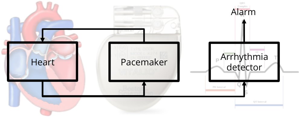
Medical data. We evaluated the resilience of traditional linear classification algorithms and the proposed algorithm using arrhythmia dataset. The arrhythmia, a.k.a irregular heartbeat, is a condition of the heart in which the heartbeat is irregular. An arrhythmia detector cooperated with logs from pacemaker can reduce stroke and death rate (Glotzer et al., 2003). To design such a detector, electrocardiogram (ECG) training data can be collected from logs of the pacemaker (Figure 2) whether ECG data is normal or abnormal (e.g., atrial fibrillation or sinus tachycardia). But, if the pacemaker is vulnerable, the training data can be tampered to hinder to detect arrhythmia, possibly leading to death.
In Table 3, we have compared the resilience of each algorithm on real medical dataset. Arrhythmia dataset (Guvenir et al., 1997), which can be found at the UCI machine learning repository (Lichman, 2013), is used for evaluating the resilience of each algorithm. The Arrhythmia dataset is preprocessed as follows. Due to the computational limitation to solve the MILP, we use 20 percent of training data (i.e., and ) and select features from 40th and 99th for training classifiers. We’ve obtained the same results as illustrated with synthetic data. SVMs algorithm outputs a classifier that misclassifies all positive or negative feature vectors under both a point attack and an overlap attack. - loss linear classification does not affect on a point attack but outputs a classifier that misclassifies all positive or negative feature vectors when an overlap attack is applied by tampering 43.2 and 42.8 percent of positive and negative feature vector, respectively. However, the majority - loss linear classification still correctly classifies the portion of positive and negative feature vectors even though about 43 percent of training data were tampered. We emphasize that values in Table 3 are not prediction results, but they are evaluated over training data, making possible. However, a higher value implies higher prediction error.
Comparison with (Kearns and Li, 1993). Kearns and Li’s paper (Kearns and Li, 1993) analyzes a binary classification problem under the malicious error (ME) model, but our paper analyzes a binary linear classification problem under a BFA, which is a general case of the ME model. Here, we compare each paper’s result by providing an example. Assume a binary linear classification problem under the ME model, where and . Kearns and Li’s paper states that if a designer wants to have the expected accuracy of , then regardless of a classification algorithm. This means at most percent of training data can be tampered to guarantee the expected accuracy. However, this does not state anything on the expected accuracy when . In comparison to this, our paper implies that, in the case of the majority - linear classification algorithm, . This means that a designer can expect the accuracy on training data that is at least . This further implies the expected minimum accuracy can be approximately when . We note that the connection between the accuracy on training data (i.e., the performance measure of this paper) and the expected accuracy (i.e., the performance measure of traditional classification) can be found in Section A.
8. Conclusions
In particularly, the incorrect decisions on CPS directly affect on a physical environment, so learning techniques under training data attacks should be scrutinized. Toward the goal of resilient machine learning, we propose a resilience metric for the analysis and design of a resilient classification algorithm under training data attacks. Traditional algorithms, such as convex loss linear classification algorithms and the - loss linear classification algorithm, are proved to be resilient under restricted conditions. However, the proposed - loss linear classification with a majority constraint is more resilient than others, and it is the maximally resilient algorithm among linear classification algorithms. The worst-case resilience bound of the proposed algorithm is then provided, suggesting how resilient the algorithm is under training data attacks.
Countermeasures. The resilience analysis on different linear classification algorithms provides us clues for countermeasures on training data attacks. Here, we briefly discuss a possible direction for countermeasures and its challenges. In general, additional algorithms can be considered to eliminate the worst-case situations in the analysis of each classification algorithm. For example, to defend against the point attack on SVMs, it might be considered to add a preprocessing step that saturates large values in training data. Specifically, if a designer knows the minimum and maximum range of features, then range can saturate the large values that contribute to the point attack. However, this might not be an effective countermeasure since the range of features is not known in general and the point attack can be conducted after the preprocessing step, not before it.
Here, we emphasize that our analysis, which is purposely focused on a classification algorithm exclusively, helps to devise countermeasures: combining a classification algorithm with a preprocessing step or using a complex classification algorithm (e.g., hierarchical approach and neural networks). We believe that the advanced algorithms work better under the training data attack in general and our analysis on the simple algorithms (e.g., SVMs) can be a building block for analyzing and devising advanced algorithms.
Future works. As a future work, the following issues are worth being considered. A more practical mixed integer linear program can speed up computational time (e.g., (Nguyen and Sanner, 2013)) and it would be promising to design and analyze multiple algorithms in tandem (one to monitor the data, one to learn a classifier). It is also worth incorporating bounded noise error and designing error on in analysis, and extending to non-linear and multiclass classification problem. Finally, to devise countermeasures, it would be promising to consider resilient algorithms that estimate attacker capabilities or model prior knowledge on attackers.
Acknowledgements.
This work was supported in part by NSF CNS-1505799 and the Intel-NSF Partnership for Cyber-Physical Systems Security and Privacy, by ONR N00014-17-1-2012, and by Global Research Laboratory Program (2013K1A1A2A02078326) through NRF, and the DGIST Research and Development Program (CPS Global Center) funded by the Ministry of Science, ICT & Future Planning. This material is also based in part on research sponsored by DARPA under agreement number FA8750-12-2-0247. The U.S. Government is authorized to reproduce and distribute reprints for Governmental purposes notwithstanding any copyright notation thereon. The views and conclusions contained herein are those of the authors and should not be interpreted as necessarily representing the official policies or endorsements, either expressed or implied, of DARPA or the U.S. Government.References
- med (2016) 2016. FBI probing after hackers cripple computer systems at major hospital chain. (Mar. 2016). http://www.cbsnews.com/news/fbi-probing-after-hackers-cripple-computer-systems-at-major-hospital-chain-medstar-health/
- jji (2016) 2016. R7-2016-07: Multiple Vulnerabilities in Animas OneTouch Ping Insulin Pump. (Oct. 2016).
- Met (2016) 2016. U.S. hospitals are getting hit by hackers. (Mar. 2016). http://money.cnn.com/2016/03/23/technology/hospital-ransomware/
- Angluin and Laird (1988) Dana Angluin and Philip Laird. 1988. Learning from noisy examples. Machine Learning 2, 4 (1988), 343–370.
- Bartlett et al. (2006) Peter L Bartlett, Michael I Jordan, and Jon D McAuliffe. 2006. Convexity, classification, and risk bounds. J. Amer. Statist. Assoc. 101, 473 (2006), 138–156.
- Biggio et al. (2013) Battista Biggio, Igino Corona, Davide Maiorca, Blaine Nelson, Nedim Srndic, Pavel Laskov, Giorgio Giacinto, and Fabio Roli. 2013. Evasion attacks against machine learning at test time. In Joint European Conference on Machine Learning and Knowledge Discovery in Databases. Springer, 387–402.
- Biggio et al. (2012) Battista Biggio, Blaine Nelson, and Pavel Laskov. 2012. Poisoning Attacks against Support Vector Machines. In Proceedings of the 29th International Conference on Machine Learning (ICML-12). 1807–1814.
- Bonaci et al. (2015) Tamara Bonaci, Junjie Yan, Jeffrey Herron, Tadayoshi Kohno, and Howard Jay Chizeck. 2015. Experimental analysis of denial-of-service attacks on teleoperated robotic systems. In Proceedings of the ACM/IEEE Sixth International Conference on Cyber-Physical Systems. ACM, 11–20.
- Brückner and Scheffer (2011) Michael Brückner and Tobias Scheffer. 2011. Stackelberg games for adversarial prediction problems. In Proceedings of the 17th ACM SIGKDD international conference on Knowledge discovery and data mining. ACM, 547–555.
- Cárdenas et al. (2008) Alvaro A Cárdenas, Saurabh Amin, and Shankar Sastry. 2008. Research Challenges for the Security of Control Systems.. In HotSec.
- Checkoway et al. (2011) Stephen Checkoway, Damon McCoy, Brian Kantor, Danny Anderson, Hovav Shacham, Stefan Savage, Karl Koscher, Alexei Czeskis, Franziska Roesner, Tadayoshi Kohno, and others. 2011. Comprehensive Experimental Analyses of Automotive Attack Surfaces.. In USENIX Security Symposium. San Francisco.
- Chen et al. (2015b) Chenyi Chen, Ari Seff, Alain Kornhauser, and Jianxiong Xiao. 2015b. Deepdriving: Learning affordance for direct perception in autonomous driving. In Proceedings of the IEEE International Conference on Computer Vision. 2722–2730.
- Chen et al. (2015a) Sanjian Chen, Lu Feng, Michael R Rickels, Amy Peleckis, Oleg Sokolsky, and Insup Lee. 2015a. A Data-Driven Behavior Modeling and Analysis Framework for Diabetic Patients on Insulin Pumps. In Healthcare Informatics (ICHI), 2015 International Conference on. IEEE, 213–222.
- Chen et al. (2013) Yudong Chen, Constantine Caramanis, and Shie Mannor. 2013. Robust sparse regression under adversarial corruption. In Proceedings of the 30th International Conference on Machine Learning (ICML-13). 774–782.
- Cortes and Vapnik (1995) Corinna Cortes and Vladimir Vapnik. 1995. Support-vector networks. Machine learning 20, 3 (1995), 273–297.
- Cretu et al. (2008) Gabriela F Cretu, Angelos Stavrou, Michael E Locasto, Salvatore J Stolfo, and Angelos D Keromytis. 2008. Casting out demons: Sanitizing training data for anomaly sensors. In IEEE Symposium on Security and Privacy (S&P). IEEE, 81–95.
- Dalvi et al. (2004) Nilesh Dalvi, Pedro Domingos, Sumit Sanghai, Deepak Verma, and others. 2004. Adversarial classification. In Proceedings of the tenth ACM SIGKDD international conference on Knowledge discovery and data mining. ACM, 99–108.
- Fawzi et al. (2014) Hamza Fawzi, Paulo Tabuada, and Suhas Diggavi. 2014. Secure estimation and control for cyber-physical systems under adversarial attacks. IEEE Trans. Automat. Control 59, 6 (2014), 1454–1467.
- Feige et al. (2015) Uriel Feige, Yishay Mansour, and Robert Schapire. 2015. Learning and inference in the presence of corrupted inputs. In Proceedings of The 28th Conference on Learning Theory.
- Feng et al. (2014) Jiashi Feng, Huan Xu, Shie Mannor, and Shuicheng Yan. 2014. Robust logistic regression and classification. In Advances in Neural Information Processing Systems. 253–261.
- Glotzer et al. (2003) Taya V Glotzer, Anne S Hellkamp, John Zimmerman, Michael O Sweeney, Raymond Yee, Roger Marinchak, James Cook, Alexander Paraschos, John Love, Glauco Radoslovich, and others. 2003. Atrial high rate episodes detected by pacemaker diagnostics predict death and stroke report of the atrial diagnostics ancillary study of the MOde Selection Trial (MOST). Circulation 107, 12 (2003), 1614–1619.
- Goldman and Sloan (1995) Sally A. Goldman and Robert H. Sloan. 1995. Can pac learning algorithms tolerate random attribute noise? Algorithmica 14, 1 (1995), 70–84.
- Goodfellow et al. (2015) Ian J. Goodfellow, Jonathon Shlens, and Christian Szegedy. 2015. Explaining and harnessing adversarial examples, In International Conference on Learning Representations (ICLR). arXiv preprint arXiv:1412.6572 (2015).
- Guvenir et al. (1997) H Altay Guvenir, Burak Acar, Gulsen Demiroz, and Ayhan Cekin. 1997. A supervised machine learning algorithm for arrhythmia analysis. In Computers in Cardiology 1997. IEEE, 433–436.
- Hadsell et al. (2009) Raia Hadsell, Pierre Sermanet, Jan Ben, Ayse Erkan, Marco Scoffier, Koray Kavukcuoglu, Urs Muller, and Yann LeCun. 2009. Learning long-range vision for autonomous off-road driving. Journal of Field Robotics 26, 2 (2009), 120–144.
- Humphreys et al. (2008) Todd E Humphreys, Brent M Ledvina, Mark L Psiaki, Brady W OÕHanlon, and Paul M Kintner Jr. 2008. Assessing the spoofing threat: Development of a portable GPS civilian spoofer.
- Kantchelian et al. (2015) Alex Kantchelian, JD Tygar, and Anthony D Joseph. 2015. Evasion and Hardening of Tree Ensemble Classifiers. arXiv preprint arXiv:1509.07892 (2015).
- Kearns and Li (1993) Michael Kearns and Ming Li. 1993. Learning in the presence of malicious errors. SIAM J. Comput. 22, 4 (1993), 807–837.
- Koscher et al. (2010) Karl Koscher, Alexei Czeskis, Franziska Roesner, Shwetak Patel, Tadayoshi Kohno, Stephen Checkoway, Damon McCoy, Brian Kantor, Danny Anderson, Hovav Shacham, and others. 2010. Experimental security analysis of a modern automobile. In IEEE Symposium on Security and Privacy (S&P). IEEE, 447–462.
- Krizhevsky et al. (2012) Alex Krizhevsky, Ilya Sutskever, and Geoffrey E Hinton. 2012. Imagenet classification with deep convolutional neural networks. In Advances in neural information processing systems. 1097–1105.
- Lanckriet et al. (2002) Gert RG Lanckriet, Laurent El Ghaoui, Chiranjib Bhattacharyya, and Michael I Jordan. 2002. A robust minimax approach to classification. Journal of Machine Learning Research 3, Dec (2002), 555–582.
- Lichman (2013) M. Lichman. 2013. UCI Machine Learning Repository. (2013). http://archive.ics.uci.edu/ml
- Madhur Behl and Mangharam (2016) Achin Jain Madhur Behl and Rahul Mangharam. 2016. Data-Driven Modeling, Control and Tools for Cyber-Physical Energy Systems. ACM/IEEE 7th International Conference on Cyber-Physical Systems (ICCPS) (apr 2016).
- Mei and Zhu (2015) Shike Mei and Xiaojin Zhu. 2015. Using Machine Teaching to Identify Optimal Training-Set Attacks on Machine Learners.. In AAAI. 2871–2877.
- Mo and Sinopoli (2010) Yilin Mo and Bruno Sinopoli. 2010. False data injection attacks in control systems. In Preprints of the 1st workshop on Secure Control Systems. 1–6.
- Natarajan et al. (2013) Nagarajan Natarajan, Inderjit S Dhillon, Pradeep K Ravikumar, and Ambuj Tewari. 2013. Learning with noisy labels. In Advances in neural information processing systems. 1196–1204.
- Nguyen and Sanner (2013) Tan Nguyen and Scott Sanner. 2013. Algorithms for Direct 0–1 Loss Optimization in Binary Classification. In Proceedings of the 30th International Conference on Machine Learning (ICML-13). 1085–1093.
- Pajic et al. (2014) Miroslav Pajic, James Weimer, Nicola Bezzo, Paulo Tabuada, Oleg Sokolsky, Insup Lee, and George J Pappas. 2014. Robustness of attack-resilient state estimators. In ICCPS’14: ACM/IEEE 5th International Conference on Cyber-Physical Systems (with CPS Week 2014). IEEE Computer Society, 163–174.
- Paridari et al. (2016) Kaveh Paridari, Alie El-Din Mady, Silvio La Porta, Rohan Chabukswar, Jacobo Blanco, André Teixeira, Henrik Sandberg, and Menouer Boubekeur. 2016. Cyber-Physical-Security Framework for Building Energy Management System. In 2016 ACM/IEEE 7th International Conference on Cyber-Physical Systems (ICCPS). IEEE, 1–9.
- Pasqualetti et al. (2013) Fabio Pasqualetti, Florian Dörfler, and Francesco Bullo. 2013. Attack detection and identification in cyber-physical systems. IEEE Trans. Automat. Control 58, 11 (2013), 2715–2729.
- Seo et al. (2014) Young-Woo Seo, Junsung Kim, and Ragunathan Rajkumar. 2014. Predicting dynamic computational workload of a self-driving car. In 2014 IEEE International Conference on Systems, Man, and Cybernetics (SMC). IEEE, 3030–3035.
- Shoukry et al. (2013) Yasser Shoukry, Paul Martin, Paulo Tabuada, and Mani Srivastava. 2013. Non-invasive spoofing attacks for anti-lock braking systems. In International Workshop on Cryptographic Hardware and Embedded Systems. Springer, 55–72.
- Sloan (1988) Robert Sloan. 1988. Types of noise in data for concept learning. In Proceedings of the first annual workshop on Computational learning theory. Morgan Kaufmann Publishers Inc., 91–96.
- Son et al. (2015) Yunmok Son, Hocheol Shin, Dongkwan Kim, Youngseok Park, Juhwan Noh, Kibum Choi, Jungwoo Choi, and Yongdae Kim. 2015. Rocking drones with intentional sound noise on gyroscopic sensors. In 24th USENIX Security Symposium (USENIX Security 15). 881–896.
- Szegedy et al. (2014) Christian Szegedy, Wojciech Zaremba, Ilya Sutskever, Joan Bruna, Dumitru Erhan, Ian Goodfellow, and Rob Fergus. 2014. Intriguing properties of neural networks. In International Conference on Learning Representations (ICLR). http://arxiv.org/abs/1312.6199
- Teixeira et al. (2010) André Teixeira, Saurabh Amin, Henrik Sandberg, Karl H Johansson, and Shankar S Sastry. 2010. Cyber security analysis of state estimators in electric power systems. In 49th IEEE conference on decision and control (CDC). IEEE, 5991–5998.
- Valenzuela et al. (2013) Jorge Valenzuela, Jianhui Wang, and Nancy Bissinger. 2013. Real-time intrusion detection in power system operations. IEEE Transactions on Power Systems 28, 2 (2013), 1052–1062.
- Van Trees (2004) Harry L Van Trees. 2004. Detection, estimation, and modulation theory. John Wiley & Sons.
- Vapnik (1999) Vladimir N Vapnik. 1999. An overview of statistical learning theory. IEEE transactions on neural networks 10, 5 (1999), 988–999.
- Wu and Liu (2012) Yichao Wu and Yufeng Liu. 2012. Robust truncated hinge loss support vector machines. J. Amer. Statist. Assoc. (2012).
- Yuan et al. (2016) Chenyang Yuan, Jérôme Thai, and Alexandre M Bayen. 2016. ZUbers against ZLyfts Apocalypse: An Analysis Framework for DoS Attacks on Mobility-as-a-Service Systems. In 2016 ACM/IEEE 7th International Conference on Cyber-Physical Systems (ICCPS). IEEE, 1–10.
- Zhang (2004) Tong Zhang. 2004. Solving large scale linear prediction problems using stochastic gradient descent algorithms. In Proceedings of the twenty-first international conference on Machine learning. ACM, 116.
Appendices
Appendix A Connection to Statistical Learning Theory
The goal of machine learning should minimize the generalization error; moreover, we believe the proposed resilience metric and generalization error are connected. To illustrate this, first, let us introduce a few standard notations from machine learning community. Let be the empirical risk of a classifier, be the expected risk of a classifier, be the empirical risk of a trained classifier, be the risk of the trained classifier, be the expected risk of the best classifier in , and be the Bayes risk. Roughly speaking, the goal of learning problem is minimizing the generalization error
The generalization error usually decomposed into two errors, called the estimation error and approximation error, as follows:
Minimizing the approximation error is related to finding a “good” hypothesis space, . We acknowledge there are many techniques for identifying a hypothesis space including structural risk minimization, finding a regularization parameter using cross-validation, model selection, drop-out in deep learning, and manual modeling of neural network architecture. However, in our paper, we’ve assumed we have a “good” , meaning contains the true classifier so approximation error always equals zero. Furthermore, since we’ve assumed there is no noise (or uncertainty) so Bayes risk is also zero – which implies that .
If we assume empirical risk minimization as a learning algorithm, the estimation error can be further decomposed as follows:
In statistical learning theory, it is known that the first term (i.e., 11 1 some literatures call this term generalization error.) and the second term (i.e., ) converge in probability to zero due to Vapnik-Chervonenkis (VC) theory. Thus, if the number of training data goes to infinity and if empirical risk minimization is used as a learning algorithm, the estimation error converges in probability to zero. Furthermore, this implies that converges to zero since (as described above) by assumption.
We can consider the resilient learning problem in a similar fashion; the resilient learning problem is minimizing the estimation error
where is a classifier trained over tampered training data. Similar to the traditional approach, this error can be decomposed as:
As before, the term converges in probability to zero due to VC theory and , which implies . But, we believe the behaviors of the term and are uncharacterized and in this work, we consider the term . Note that based on the notations in paper,
where , suggesting the resilience metric Eq. (3) is connected to existing statistical learning theory. Note that we’ve used -norm and instead since our setup also is used in literatures and we think it describes the behavior of the empirical risk of a trained classifier better when an attack is severe (in other words, is large).
Appendix B Proofs on Lemmas, Propositions, and Theorems
In this section, we describe the proofs of propositions and theorems stated in the paper, including supporting lemmas. For the notational simplicity, we use the following shorthands. Let , , and . Let such that . When a - loss function is used, a set of classifiers has a same empirical risk. We denote, given , the class of classifiers that has a same empirical risk with as . In this case, only the representative, , is considered so that, for example, if there are three different classes of classifiers, they are simply called three different classifiers. Figures used in proofs represent training data, where the point means the overlap of the annotated number of feature vectors. The positive and negative feature vectors are color-encoded in blue and red, respectively. Set notations in the papers can be generalized to multiset notations. In the following proof, we assume all sets defined are multisets to handle duplicated training data pairs, which can happen if .
B.1. Lemmas
Lemma B.1.
For all , , , and , the following is true:
Proof.
First, for any classifier, , can increase compared to if an attacker maliciously manipulates training data. Also, the amount of the empirical risk increased is at most depending on the choice of the attacker. Formally,
where . Likewise, .
Next, for any classifier, , can decrease compared to if an attacker helps for classification. Also, the amount of the empirical risk decreased is at most depending on the choice of the attacker. Formally,
where . Likewise, . ∎
Lemma B.2.
Let be a convex loss function and be linear. For all , , and , there exists such that .
Proof.
Let , where , is convex, and , which is a usual setup for convex losses (Bartlett et al., 2006).
By the convexity of and ,
Given , , and , can be chosen such that since can increase arbitrarily by moving toward the direction of the normal vector of if or the opposite direction of the normal vector of if . This implies for some . ∎
B.2. Proposition and Theorem Proofs
B.2.1. Theorem 1
Proof.
Let for the notational simplicity of this proof, and , where . Assume that is lower-bounded by , it is a monotonically non-increasing function, and for some scalar . Note that the assumptions are generalized from the assumptions on convex losses (Bartlett et al., 2006) to cover non-convex ones.
Theorem 1 is formally stated as follows:
| (13) |
Assume . we partition the type of loss functions into two classes. One class is the set of the loss function that has a “flat tail”. Formally, it is the set of such that for some negative and some scalar . Call this set . The other class is the set of the loss function that has a “not-flat tail”. Formally, it is the set of such that for any negative . Call this set . We claim that and illustrated in Figure 6 makes or for any . In Figure 6(b), we denote feature vectors annotated by as and the point means a set, , of -pairs of . Also, the three points are collinear.
First, assume . As illustrated in Figure 6, we consider two classes of classifiers, and , where misclassifies all feature vectors annotated by but correctly classifies others and misclassifies all feature vectors annotated by but correctly classifies others. By the definition of , the followings are true:
Also, from and ,
This implies and . Thus, for some and all .
Next, assume . Same as before, as illustrated in Figure 6, we consider two classes of classifiers, and . By the definition of , an attacker can choose such that
This is because the left term can be arbitrarily large if an attacker moves to the right side in Figure 6(b). However, the right term cannot be arbitrarily large since any correctly classifies . Here, let . Thus, the following is true:
This implies . Thus, for some and all . Likewise, if , then for some and all . Therefore, Equation (13) is true. ∎
B.2.2. Theorem 2
Proof.
Assume . Since in Theorem 1 provides a theoretical upper bound of , . Also, by the definition of the maximal resilience attack condition, . Therefore, . ∎
B.2.3. Proposition 1
Proof.
Let for the notational simplicity of this proof. The proposition is formally stated as follows:
We prove that if and , then is not perfectly attackable. Since an attacker cannot attack any point, and . This implies and , which implies is not perfectly attackable.
We prove that if or , then is perfectly attackable.
First, assume . Consider and illustrated in Figure 5. An attacker converts to by moving one positive data pair, , to the right side, such that three points are collinear as in Figure 5(b).
Given , there are six classes of classifiers, , where and are classifiers illustrated in Figure 5(b). By Lemma B.2, an attacker can choose such that , where
From this, the following is true:
where . Thus, . This implies there exists a classifier that is trained over can misclassify all positive or negative feature vectors in , i.e., or for some . Therefore, is perfectly attackable. ∎
B.2.4. Proposition 2
Proof.
Let . Proposition 2 is formally described as follows:
Prove that if the conditions, , , , or , satisfies, then is perfectly attackable.
First, assume . To show is perfectly attackable, it is enough to find and for all and that make perfectly attackable. Consider and described in Figure 6. By a BFA, can be represented as in Figure 6(b). Note that the attacker does not move negative feature vectors even though it may have the ability to do that. Since , . This means there exists that misclassifies all positive or negative feature vectors in , i.e., or for some . Therefore, for all and , there exist and that make perfectly attackable. Likewise, if , for all and , there exist and that make perfectly attackable.
Next, assume . For all and , there exist and that make perfectly attackable as illustrated in Figure 7. When is trained over , one possible optimal classifier can be as represented in Figure 7(b) among eight different classifiers except for and . Since , and , the empirical risk of is as small as and . Thus, any classifier, , has or , which implies for all and there exists and that make perfectly attackable. Likewise, for all and , if , then is perfectly attackable for some and .
Therefore, for all the above mentioned four cases, there exist and that make perfectly attackable. ∎
B.2.5. Theorem 3
Proof.
Let , , where , and Formally, show the following statement:
First, prove that if the conditions, and , hold, then is feasible and resilient to -BFA for all . To prove , it is enough to show includes at least one element for all , , , and . Consider . By Lemma B.1 and the conditions,
Likewise, , suggesting for all , , , and .
Since , prove that is resilient. By the definition of ,
for all , , and . Thus,
by Lemma B.1, the majority constraint, and the conditions. Likewise, . Therefore, for all , , , and , is resilient to -BFA if .
Next, prove that if is feasible and resilient, then the conditions, , hold. Equivalently,
To show this, it is enough to find and for all and that make infeasible or perfectly attackable. Assume is feasible and check whether it is perfectly attackable. The proof is same as proving is perfectly attackable if or in Section B.2.4. The main difference is the feasible set. Here, is used instead of . But, we can use the same proof to prove is perfectly attackable since in Figure 6(b) still satisfy the majority constraint such that .
Therefore, there exist and that make perfectly attackable if or . ∎
B.2.6. Theorem 4
Proof.
Let , , where , and for the notational simplicity of this proof.
Show that the worst-case resilience of is tightly bounded. Formally,
| (14) |
Note that the proof of Theorem 3 implies if and , then is feasible.
(bounded) First, we prove that the worst-case resilience of is bounded. The optimality of with Lemma B.1 implies the following:
where is a slack variable to satisfy the majority constraint such that .
If , maximizes . Thus,
| (15) |
If , can be the smallest non-zero scalar such that . Thus,
| (16) |
From the above two cases,
| (17) |
Likewise,
| (18) |
Therefore, for all , , , , and , Equation (14) is true.
(tight) Next, we prove that the worst-case resilience bound is tight. To prove the tightness, we show there exist , , and by which the equality of Equation (14) holds for all and if is linear, , and .
The examples of , , and are illustrated on Figure 8. Figure 8(a) shows and the corresponding optimal classifier . Figure 8(b) shows and the projected optimal classifier trained over . Figure 9 represents from which is obtained. Note that the annotated number of positive and negative feature vectors are the difference from the original numbers in Figure 8; i.e., the blue dot has number of positive feature vectors as originally denoted and the red dot has number of negative feature vectors.
If , let . There are 16 different linear classifiers that separate five dots in Figure 9. Each classifier has an empirical risk, , among , , or is infeasible due to the majority constraint. Thus, can be optimal. From this, that satisfies the equality in Equation (15). Likewise, we can find , , and such that .
If , let . There are 16 different linear classifiers that separate 5 dots in Figure 9. Each classifier has an empirical risk, , among , , , or is infeasible due to the majority constraint. Thus, can be optimal. From this, that satisfies the equality in Equation (16). Likewise, we can find , , and such that .
Appendix C Proof on Mixed-Integer Linear Program for 0-1 Linear Classification
In this section, we derive Mixed-Integer Linear Program (MILP) for 0-1 linear classification algorithm from the standard 0-1 linear classification problem.
Proof.
The 0-1 linear classification problem is minimizing the misclassification error of a classifier over training data, or equivalently the sum of a 0-1 loss of a classifier over each training data pairs, according to
We introduce new binary variable such that . Since assuming , if , and if , the equivalent problem (by introducing equality constraints) is as follows:
| s.t. |
Next, we introduce new variables to convert the indicator function into a real-valued function. The equivalent problem is as follows:
| s.t. |
This problem is equivalent to the previous one since the optimal values are identical. Specifically, if there are such that for some , then in the previous problem if and only if and in this problem. Likewise, if there are such that for some , then in the previous problem if and only if and in this problem. Thus, for all .
To remove the indicator function, we introduce new slack variable . Also, let , assuming is sufficiently large. The equivalent problem is as follows:
| s.t. | |||
where is a sufficiently small value. To prove the equivalence, check whether the optimal solution of the previous problem and this problem are same. Let and be the optimal solution of the previous and this problem, respectively. If there are such that for some , then and in the previous problem, and , , and are optimal solutions in this problem, resulting . If there are such that for some , and in the previous problem, and , , and are optimal solutions in this problem, resulting . Thus, for all .
To reduce the number of optimization parameters, we consider the following problem:
| s.t. | |||
The previous problem and this problem are equivalent since the optimal solution on for both problems are same. Specifically, let and are the optimal solution of the previous and this problem, respectively. First, assume . This implies and . Since, in this problem, implies , . Likewise, implies . Next, assume . This implies and . In this problem, implies or . Thus, . Likewise, implies . Therefore, .
Finally, if each constraints are divided by , then we have the following MILP.
| s.t. | |||
and if let , , and , the final MILP is obtained. ∎