An Empirical Study on Writer Identification & Verification from Intra-variable Individual Handwriting
Abstract
The handwriting of an individual may vary substantially with factors such as mood, time, space, writing speed, writing medium and tool, writing topic, etc. It becomes challenging to perform automated writer verification/identification on a particular set of handwritten patterns (e.g., speedy handwriting) of a person, especially when the system is trained using a different set of writing patterns (e.g., normal speed) of that same person. However, it would be interesting to experimentally analyze if there exists any implicit characteristic of individuality which is insensitive to high intra-variable handwriting. In this paper, we study some handcrafted features and auto-derived features extracted from intra-variable writing. Here, we work on writer identification/verification from offline Bengali handwriting of high intra-variability. To this end, we use various models mainly based on handcrafted features with SVM (Support Vector Machine) and features auto-derived by the convolutional network. For experimentation, we have generated two handwritten databases from two different sets of 100 writers and enlarged the dataset by a data-augmentation technique. We have obtained some interesting results.
Keywords:
Intra-variable handwriting , Writer identification , Writer verification.1 Introduction
“Handwriting" is basically a kind of pattern. However, from the pre-historic era, it bears the connotation of human civilization. The handwriting instrument progressed from finger and wedge (on clay/sand and stone-based medium) to quill, pencil, fountain/ball-point pen (on parchment, papyrus/paper), and again finger (on the touch-screen of a smart device). Though the world is going fast towards a paperless e-world, “handwriting remains just as vital to the enduring saga of civilization (–Michael R. Sull)".
For computer scientists, automated analysis of handwriting is a recognized field of study owing to the ever-increasing complexity of extreme variations and having positive impacts on the fields of Forensics, Biometrics, Library Science and Data Science.
The handwriting pattern varies with person due to individual writing style. This may be termed as inter-class variance. It is also noted that handwriting samples of a single person may vary extensively with various factors such as mood, time, space (geographical location), writing medium and tool. This is referred to as intra-class variance. Sometimes, these inter-class and intra-class variations are termed as “between-writer" and “within-writer" variability, respectively [43]. Even for excessive stroke variation among handwritten specimens of a particular writer, the writer and others having long exposure to his/her writing may still recognize it. Some implicit stroke characteristics may be the reason behind this ability.
In the field of forensics and biometrics, verifying/identifying a writer from a handwriting sample is sometimes essential (e.g., in the case of the “2001 anthrax attacks"). Now-a-days, computer-assisted automated analysis is also quite popular in this application. Writer verification is a task used to authenticate a given document whether it is written by a certain individual or not. In writer identification, the goal is to match the writers to their handwriting specimens. The target of the writer identification/verification task is to maximize inter-variability and to minimize intra-variability.
The workflow of writer identification and verification approach is shown in Fig. 1. Here, we have a database of handwritten texts with its known authors/writers. A query text sample Text-i is input to the writer identification system to obtain its writer-id (Writer-i) as an output with a certain degree of accuracy where the database provides support for the retrieval. In the writer verification system, two text samples Text-i and Text-j are fed to decide whether they are written by the “Same" or “Different" persons. The Text-i is a query sample to be verified and the Text-j may be fed from the database of known authors.

In the document image analysis literature, interest has grown in the area of automated writer identification/verification for the last four decades. A detailed survey of the reported research works on this topic up to the year 1989 have been compiled in [51]. Recent advancements on writer identification/verification can be found in [55, 68]. Most of the past research work [51, 55, 68] has focused on ideal handwriting generated in normal circumstances without paying much attention to the intra-variability.
However, a situation may arise where an author needs to be verified based on a quickly written, unadorned handwritten manuscript, whereas only regular neat/clean handwriting with known authorship is available in the training database. Similar situations may occur where we need to identify the writer from unclaimed tidy handwriting, but the available database contains only careless untidy writing. In such a situation, the available writing of the person in the database and the test document written by the same individual can be highly dissimilar. In Fig. 2, two sets of intra-varied handwritten sample of two individual writers are shown. Here, for example, we may need to verify whether the sample of Fig. 2.(B1) is written by Writer-B, on the basis of B’s handwriting of say Fig. 2.(B3).
(A1) (B1)
(B1)
(A2) (B2)
(B2)
(A3) (B3)
(B3)
In this paper, we focus on the situation of intra-variation of individual handwriting to perform writer identification/verification. Ideally, within-writer variation should be less than the between-writer variation, which is the basis of the writer identification/verification task [43]. However, where the intra-variation is relatively higher (refer to Fig. 2), we need to find some handwriting features less sensitive to intra-variability and more sensitive to inter-variability.
We have generated two sets of database of intra-variable handwriting to deal with such realistic scenarios of writing identification/verification. Our database contains offline handwriting of Bengali (endonym, Bangla) script which is a fairly complex Indic script and used by more than 250 million people [49, 10]. Recent advancements in writer identification on Indic scripts have been reported in [13]. The general features of Bengali script can be found in [10]. In connection with writer identification, some useful characteristics of Bengali handwriting are mentioned in [13], for example, matra/headline, delta, hole, coil shape, etc. We have noted that these Bengali handwriting characteristics along with classical handwriting characteristics (inter-text-line and inter-word gap, text-line skew, word/character slant, height/width of a character, text main-body height, character formation, etc.) usually vary with writing.
In our generated database, the intra-variation is relatively higher than most of the existing databases in the literature [68], as confirmed by some handwriting experts. Therefore, here, we need to find some handwriting features which can decrease the intra-variability and increase the inter-variability.
The applicability of this work is as follows. First, it will be helpful in the fields of forensics and biometrics for writer identification and verification. Second, this work studies the impact of working with absent data, i.e., when a particular type of individual writing is absent in the training set, how the system performs while testing with that type. Third, this work may be useful in some applications of cultural heritage and library science. When some unpublished manuscripts of a scholar are found, the authorship is usually verified [32]. Now, for the case of newly-discovered manuscripts, if they contain some unknown writing styles of the scholar, our work may provide some insights to analyze the authorship. Fourth, this work may have a modest understanding of the progress of some diseases such as Parkinson’s, Alzheimer’s, Dysgraphia, Dyslexia, Tourette syndrome, etc., which affect handwriting. Here, before and after the disease progression, handwritten specimens have high intra-variability and provide some applicability of our work.
In this paper, we analyze the intra-variable handwriting for writer identification and verification tasks. The writer identification task is perceived as an -class classification problem to classify handwritten documents in number of writer classes. On the other hand, writer verification is perceived as a binary classification, where a document is marked with “Same" or “Different" class, if it is written by the same or different writer of the given document, respectively. For these tasks, we extract two types of features, handcrafted and auto-derived [42], from an offline handwritten text sample set. Then the extracted features are classified to identify/verify a writer. In writer identification, SVM (Support Vector Machine) is used for handcrafted features and some deep neural models are used for auto-derived features. In writer verification, we employ some similarity metrics on handcrafted and auto-derived features.
Our contribution to this paper is the study of writer identification/verification on the intra-variable handwriting of an individual. Such a rigorous investigation is the earliest attempt of its type. For this study, we have generated two databases containing intra-variable handwriting in a controlled and uncontrolled way. The subgrouping of the uncontrolled database with respect to intra-variability is rather new. Here, the handwritten pages of the uncontrolled database are initially clustered with some deep features, and then finally grouped by confirmation of a classification technique which is pre-trained by the controlled database. We also propose two patch selection tactics to provide the input to the deep architectures without any normalization. Moreover, two writer identification strategies are introduced here, which are relatively new. The data augmentation technique is also a new addition here with respect to the offline handwritten data.
The rest of the paper is organized as follows. Section 2 discusses related work and Section 3 describes the experimental dataset generation procedure. Then Section 4 mentions the preprocessing step before entering into the methodology. After that Section 5 and Section 6 describe the handcrafted and auto-derived feature extraction techniques, respectively. The writer identification procedure is discussed in Section 7, followed by Section 8 with a description of the writer verification process. The subsequent Section 9 is comprised of experimental results and discussions. Finally, Section 10 concludes this paper.
2 Related Work
With our both online and offline searching capacities, we have not found any direct work on intra-variable handwriting for writer identification/verification. In this section, at first, we cite some slightly related works mentioning intra-variability in handwriting. Then we briefly discuss some interesting work on writer investigation (i.e., identification/verification).
2.1 Intra-variability in Handwriting
The handwriting of a person may change for using various writing instruments. The handwriting alteration of a person using a pen and pencil has been studied in [31]. Hilton [46] reported that some pens can suppress the writing characteristics of an individual and may introduce intra-variability.
The handwriting of a person may change with the writing surface, more precisely, by the friction between the writing medium (paper) and tool (pen). Gerth et al. [54] studied this within-writer variability when writing was performed on paper and a tablet computer.
Handwriting also changes with time span and the age of a person [39, 35]. Speedy writing in excitement, or writing with a stressed mind may degrade the writing quality, thus produces within-writer variability [39, 6].
Some diseases such as Parkinson’s, Alzheimer’s, etc. affect the handwriting of an individual [35, 28]. Therefore, before and after such diseases, the writing shows intra-variability.
Alcohol consumption also changes the individual’s writing style and provides an example of intra-variable handwriting [22].
Such mechanical (e.g., writing instrument, surface, etc.), physical (e.g., illness, aging, etc.), psychological (e.g., excitement, anger, mood, etc.) factors may cause large individual handwriting variation [39].
2.2 Writer Investigation
The root of writer analysis can be found around 1000 B.C. when a few Japanese scholars studied the bar formation in writing to judge personal characteristics [53]. However, with the boom of automation, during the late 20th century, such investigations had also started to be automated. In the beginning of the 21st century, the “9/11 attacks” and “2001 anthrax attacks” have escalated automated writer identification/verification research.
In the document image analysis domain, automated writer investigation research is being performed during the last four decades. Plamondon and Lorette [51] surveyed major works in this field up to the year 1989. After that, the offline writer investigation research up to the year 2007, is described in [43]. The recent advancements in this field can be found in [68]. The writer investigation research work on Indic scripts is discussed in [13]. However, most of the past research has dealt with ideal handwriting without degradation [51, 43, 68]. But, a handwritten page may contain various artifacts such as struck-out/crossed-out writing [15, 9, 1], doodles [12], ruled lines, printed text, logos, stamps, etc. [30].
Chen et al. [30] studied the impact of ruled line removal on writer identification. They [30] showed that the performance improved by retaining, instead of deleting the ruled lines. Another work in [15] reported the effect of struck-out texts on writer identification. The authors [15] experimentally showed that the presence of struck-out texts in a handwritten document degrades the writer identification performance. A preliminary work on crossed-out text removal with its effect on writer identification is presented in [1].
3 Experimental Dataset
For our experimental analysis, we needed a database of intra-variable handwritten samples of each writer. We did not find any such publicly available database. Therefore, we had to generate a new database containing such handwriting specimens. We made two offline databases on the basis of a handwriting collection strategy, namely controlled and uncontrolled databases.
3.1 Controlled Database ()
In this case, all volunteers chosen for supplying data were aware of the modality of our experiments. For controlled database collection, we focused on intra-variability occurring mostly due to writing speed [36]. It is noted that typically speedy writing is more distorted than the usual handwriting of a writer, and this inference was confirmed by some handwriting experts.
Collecting previously written samples at various speeds from many writers is quite challenging, since no one typically monitors and records his/her writing speed unless required for a specific reason. Therefore, we collected handwriting under a controlled setup, as follows.
All volunteers were instructed to write at various speeds. At first, they were advised to write at their normal speed of writing. Then they were instructed to write faster than their normal writing speed. Finally, they were requested to write at a slower speed than normal. We labelled these as medium (or, normal), fast, and slow sets of handwriting samples, respectively.
At the stage of full-page writing, we noted the total time of writing using a stop-watch and computed the total length of writing strokes on a page. The handwriting speed in a full page is calculated as stroke length per unit time, i.e., . The stroke length is computed from counting the number of object pixels from the thinned version of the writing strokes. For thinning purpose, the Zhang-Suen thinning method [61] was used which worked better than some other techniques [41]. Additionally, in the thinned version, a spurious branch having length less than half of the average stroke-width is pruned.
The reaction time ( 200 millisecond) [5] for using a stop-watch is negligible with respect to the objective of our task. We prepared our experimental setup to write on a white 70 GSM () A4 page and placing it on a horizontally plane surface with a smooth ball-point pen having black/blue ink. We created our database in offline mode, and did not use any digital pen/surfaces which could obstruct the individual writing habits. Here, our primary aim is to capture the intra-variability of handwriting, on which our technique can work adequately without using accurate, ultramodern speed measuring instruments.
For a writer , a fast handwritten page is chosen where handwriting speed (, a scalar quantity) is greater than a threshold , i.e., . For slow handwriting, , where is another threshold. The medium handwritten page is chosen where . The medium or normal handwriting speed is captured at first from multiple handwritten pages of a writer . We calculate mean () and standard deviation () of medium speed from these pages. Here, we use and . We set , which is decided empirically.
Each writer wrote multiple pages which were ordered in terms of the writing speed. We chose top speedy two pages from the fast handwritten samples, two lowest-speeded pages from the slow writing, and middle-speeded two pages from the medium writing.
Although many volunteers contributed for our database generation, we chose 100 writers whose handwriting patterns varied structurally due to writing speeds, as advised by some handwriting experts. This is performed in order to generate a database of intra-variable handwriting.
The writers were native Bengali from West Bengal, India. The finally selected 100 writers were in the age group of 12-42 years having academic backgrounds from secondary school to university level. The ratio of male to female writers in this database is 14:11.
This controlled dataset () contains 600 pages where each writer contributed 6 pages of Bengali handwriting. Among 6 pages, 2 pages are of fast handwriting speed, 2 pages are of medium and the remaining 2 pages are of slow speed. In other words, we have 3 sets of handwriting namely (fast), (medium), (slow), each containing 2 handwritten pages of every 100 writers.
3.2 Uncontrolled Database ()
For generation of the uncontrolled database, the writers should be unaware of our experiments before the data collection. However, people generally perform their daily writing at a normal pace using various pens and papers, and a uniform data collection setup is missing. Here, we came up with a different strategy for this type of database generation.
After discussions with some handwriting experts, we note that in real-life school examinations, the students generally write at various speeds, since the examination time is limited and the usual target is to score good marks by answering all questions within that stipulated period. Therefore, the students/writers are in a hurry when the clock is ticking towards the end of exam. However, here some behavioral/psychological aspects [7, 36] may influence intra-variable handwriting, besides the writing-speed, due to anxiety, nervousness to finish, panic of a low score, stress to recollect the answer, etc.
Therefore, we have selected a real school-exam scenario to collect suitable data by maintaining uniformity for this data collection. Some details of such situation are as follows:
i)Time: The examination duration was fixed as three hours. Here, the time works as a constraint to ascertain the increase/decrease of writing speed and individual variability.
ii)Question type: We selected a 100-mark Bengali literature examination paper, where most of the question types were broad subjective to be answered in many sentences.
iii)Script: The answers were to be written in Bengali script.
iv)Paper: For writing the answers, white pages of 70 GSM () with a fixed size of 215.9 355.6 were provided.
v)Pen: The writers used their own pens. Most of the pens were of black/blue ink with 0.5 - 1.0 ball-point tip.
vi)Writer: The writers were native Bengali from West Bengal, India, and students of VIII - XII grade Bengali-medium public schools. Their age ranged between 13 - 19 years. All these writers were different from the volunteers participated in controlled database generation.
The exam marking was performed by school teachers. For our task, we chose the answer script of a student who scored at least 40% and wrote at least 6 full pages. A total of 153 writers were chosen in this way. Among these writers, 67 persons wrote 6 pages each, 11 persons wrote 7 pages each, 54 persons 8 pages each, 21 persons 9 pages each. Therefore, 153 writers contributed a total of 1100 pages.
Now, we have 1100 unlabelled pages of 153 writers. We label each page in one of the 3 groups of intra-variable writings, say, , and . For this grouping, at first, we use auto-derived feature-based clustering techniques, as follows.
We use the front part of GoogLeNet [19] for feature extraction, since this architecture provides encouraging accuracy with comparatively lesser dimension of feature vector [44]. From each page, an number of text-patches of size 224 224 is chosen arbitrarily. This is set empirically to 400. For each patch, we have obtained 1024-dimensional deep feature vector from the avg pool layer of GoogLeNet [19]. For clustering, we choose various clustering algorithms such as K-means, Fuzzy C-means, Minibatch K-means, Expectation-Maximization with Gaussian-Mixture-Models (EM with GMM), and Agglomerative Hierarchical Clustering (Agglo_Hierarchical) [2].
Let us assume that pij denotes patch of page. Actually, pij represents a 1024-dimensional feature vector obtained from patch of page. For p1j, we obtain a cluster plot CL1 by patch1’s of all the 1100 pages. Similarly, cluster plot CL2 is obtained from patch2’s of all 1100 pages. And so on, patch400’s of all 1100 pages produce cluster plot CL400. These 400 cluster plots are ordered with a corresponding patch; i.e., patchi’s (or, the patch) of all pages produce CLi. Moreover, we obtain 600 (fixed empirically) cluster plots unordered with patches which are chosen arbitrarily. Therefore, we now have 1000 () cluster plots. Each cluster plot contains 1100 patches (i.e., patch-based feature points), where each patch represents each of the 1100 pages. From these 1000 cluster plots, using the majority rule, we label each page into three groups/clusters , and . For example, suppose in all the 1000 cluster plots, majority of the patches of page1 (pi1) fall in the cluster ; then the page1 is put into the group .
To find which clustering algorithm among K-means, Fuzzy C-means, Minibatch K-means, EM with GMM, and Agglo_Hierarchical, would work well for intra-variable handwriting, we use an external evaluation criterion, called NMI (Normalized Mutual Information) score [16]. For this, we perform a similar feature extraction strategy and clustering techniques on the controlled dataset , which contains the ground-truth. Employing various clustering techniques on , we have obtained the NMI scores, as presented in Table 1. The Agglo_Hierarchical method worked well on , so we use this clustering technique here also on uncontrolled data.
| Clustering method | NMI score |
|---|---|
| K-means | 0.637 |
| Minibatch K-means | 0.610 |
| Fuzzy C-means | 0.646 |
| EM with GMM | 0.679 |
| Agglo_Hierarchical | 0.684 |
Up to this point, the 1100 unlabelled pages of 153 writers are clustered into 3 groups (, and ) using an unsupervised clustering technique (Agglo_Hierarchical).
Now, we classify the 1100 pages into 3 classes (, and ) supervised by the controlled database . For this classification, we use GoogLeNet due to its promising performance in other computer vision related tasks [19]. Here also, we arbitrarily choose (, fixed empirically) number of text patches in a page and input to the GoogLeNet. A page is classified into a certain class where the majority of its patches fall.
To assess the efficiency of the GoogLeNet on intra-variable handwriting, we perform a 3-class classification experiment on to classify in , , sets/classes due to having the appropriate ground-truth. For this, we divide into training, validation, and test sets in the ratio of 2:1:1. The performance on the test set of for this 3-class classification problem is 96.87%, which is quite satisfactory for our task.
For classification of uncontrolled handwritten samples (1100 pages), we perform training on the entire controlled database and test on these 1100 pages. After this classification, we have obtained the members of 3-classes , and .
Our intention is to generate 3 sets (, and ) of samples containing intra-variable handwriting of an individual. Therefore, each of these 3 sets must contain handwriting samples of every writer.
From the unsupervised clustering, we obtain , and sets. From supervised classification, we get the sets , and . From 153 writers, we choose a certain writer who has at least 2 handwriting samples in each of the , , sets and the same 2 samples in each of the corresponding , , sets. Finally, these samples of a writer are put in , and sets, respectively. Out of 153 writers, this constraint is successfully satisfied by 104 writers. Furthermore, we take advice from some handwriting experts and finally choose 100 writers from the 104 writers.
Our uncontrolled database () contains 3 sets (, and ) of intra-variable handwriting samples of 100 writers. Each of the , and sets contain 2 samples per writer. Therefore, similar to the controlled database , this uncontrolled database also contains 600 pages in total. The ratio of male to female writers in is 31:19.
In this uncontrolled database, we observe that the handwriting of most students becomes structurally more distorted and unadorned in the latter pages of the answer booklet.
4 Preprocessing
All the handwritten pages were scanned by a flat-bed scanner at 300 ppi (pixels per inch) in 256 gray-values to obtain digital document images. In the preprocessing stage, we label the components of a handwritten document image using a relatively faster single-pass connected component labeling algorithm [25]. The text region is extracted after removal of the non-text components if present any, using the method of [12]. In the text region, the struck-out texts are also deleted by employing the method of [9], since the presence of struck-out text impedes the usual writer identification performance [15]. However, the style of strike-out strokes [9] may be utilized for writer inspection, which is out of the scope of our current work. Very small sized components such as dots, dashes, commas, colons etc., and noise are also removed. The text-lines and words are segmented using an off-the-shelf 2D Gaussian filter-based method GOLESTAN-a, as discussed in [45]. Character level segmentation is also performed using a water reservoir principle-based method [62].
5 Handcrafted Feature Extraction
A writer identification task can be viewed as a multi-class classification problem, where the task is to assign the writer-id to the unknown handwritten specimens. Similarly, writer verification can be perceived as a binary classification problem where the task is to answer yes/no to a questioned handwritten sample as to whether it has been written by a particular writer. The features used for these tasks are described in this section and the following section. We employ both handcrafted features and auto-derived features [42]. Handcrafted features are required to be predesigned explicitly in the traditional way, whereas auto-derived features do not have any explicit design.
The extracted handcrafted features are discussed as follows.
5.1 Macro-Micro Features ()
The macro and micro features of Srihari et al. [59] are quite popular since those were very effective in writer identification from handwritings of 1500 U.S. population having various ethnic groups/ages/genders. Here, we adopt this set of features for our task.
Initially, we choose the macro feature vector, described in [59], which contains 11 features: gray-level entropy (), gray-level threshold (), count of black pixels (), interior/exterior contour connectivity (-), vertical/negative/positive/horizontal contour slope (-), average slant and height of the text-line (-). From [59], we note that the features , , and are related to the pen pressure. Here, and reveal the writing movement. The features , , , and are related to stroke formation. The feature represents the writing slant and is related to the text proportion.
Two paragraph-level macro features are also considered: height to width ratio of a paragraph, i.e., aspect ratio () and margin width (). Three more word-level macro features are also employed, which are upper zone ratio (), lower zone ratio () and length (). We calculate these paragraph and word-level features over a page and take the average value.
The character-level micro features contain 192-bit gradient, 192-bit structural and 128-bit concavity features, concatenated into a 512-bit feature. The detailed description of these features can be found in [59]. We modify this micro feature slightly to get a page-level feature vector. From a page, we obtain the histogram of this 512-bit feature and normalize it by the character count.
The macro and micro features are concatenated to generate the feature vector .
5.2 Contour Direction and Hinge Features ():
For writer identification, stroke direction and curvature-based features have been reported to work well [51, 68]. Therefore, we use here the famous contour direction and hinge distribution of handwritten strokes proposed by Bulacu and Schomaker [43].
Along the writing stroke contour, an angle () histogram is generated and normalized into a probability distribution . From the horizontal direction, the angle () is calculated as:
| (1) |
where, and denote the row and column indices of the object pixel. The depends on stroke-thickness and is fixed as 5 in [43]. In our task, is data-driven, and worked well for , where is the average stroke-width and is the standard deviation of stroke-width in a page. The number of histogram bins () is set as 12 within the range of . Hence, per bin is engaged. Clearly, the dimension of this feature or is 12.
In [43], for the contour hinge feature , two contour fragments, joined to a common end, making angles and (where, ), spanning all four quadrants (), are considered. A normalized histogram is generated with a joint probability distribution . Similar to [43], the number of histogram bins () is set to 12, leading to -dimensional feature vector.
By concatenating and , we obtain .
5.3 Direction and Curvature Features at Keypoints ()
We intend to ascertain some similarities between handwriting specimens of an individual. Therefore, we focus on some points of interest, i.e., keypoints (), on the handwritten strokes. These keypoints are obtained by combining some structural points (i.e., start/end, branch and curved points) and SIFT (Scale-Invariant Feature Transform) keypoints on Bengali handwritten ink-strokes, as described in [13].
Here, our plan is to observe the movement of writing strokes on these keypoints, and therefore, we capture the stroke direction and curvature at the keypoints. For direction and curvature feature extraction from offline handwritten strokes, we use the idea of “The NPen++ Recognizer” [58] which deals with online handwriting.
We calculate the writing direction between two connected keypoints and in terms of Cosine and Sine values and use them as features and , respectively.
| (2) |
| (3) |
where, and are the row and column indices of , and
.
The curvature of a writing stroke is the angle made by the line fragments (from to ) and (from to ). The Cosine and Sine values of this angle are calculated and employed as features and , respectively.
| (4) |
| (5) |
For each of these four features (, , , ), we generate separate normalized histograms spanning the range of [-1, 1] for a number of bins . Therefore, the dimension of each feature vector is 200.
Concatenating features , , and , we get .
6 Auto-derived Feature Extraction
The auto-derived features are mainly extracted using a convolutional neural network (CNN). The convolutional architecture generally contains two parts: front and rear. The front part typically extracts the features. The rear part is used for classification (refer to Section 7.2).
The front part of the CNN takes an input image. We use some patch-based strategies to feed fixed sized input images [63]. Here, we do not use any image normalization, since it impedes the writer identification performance [8]. The patch selection is not performed through the classical sliding-window technique, since the text-lines are not skew-normalized. Sliding a window horizontally through the middle of the text-line (main text-body height) is conceivable, but the information may be lost for several cases such as for highly skewed text-lines, for overlapping text-lines with lesser inter-text-line gaps, etc.
Here, two types of patches are selected as follows.
(a) patchchar: We already have the character-level information from the pre-processing stage. We find the center of gravity (CG) of a segmented character image. Then we take a window centering the CG, and consider it as a character-level patch, say patchchar.
(b) patchallo: We have obtained some keypoints on writing strokes, as mentioned in Section 5.3. A neighboring window of size centered at a keypoint is used as a patch. This patch is an allographic-level patch, say patchallo.
From a text sample, all the patchchars and patchallos are extracted. Each patchchar is fed to the front part of the CNN and a feature vector is obtained. Similarly, for each patchallo, a feature vector is generated.
In our task, the following deep-learning architectures are used separately for patchchar and patchallo as inputs.
6.1 Basic_CNN
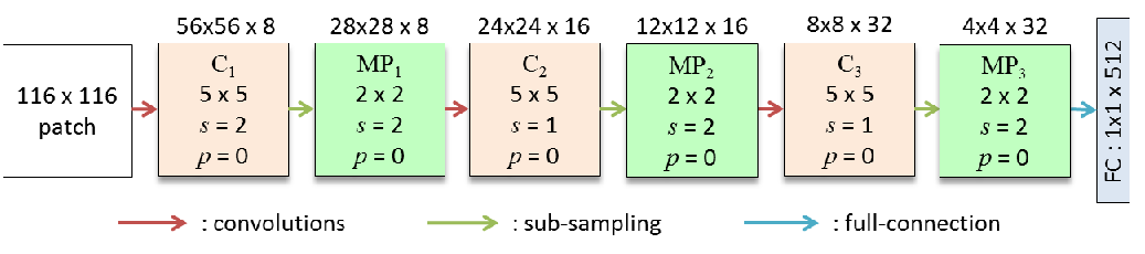
The LeNet-5 is a celebrated convolutional network that works well on various machine learning problems [69]. Our Basic_CNN architecture is primarily influenced by this LeNet-5 and provides an initial flavor of a deep learning model for our task. Here, we use 3 convolutional layers (Ci), each followed by a sub-sampling (max-pooling, MPi) layer. The used feature map count with map size, filter size, stride (), padding () values are shown in Fig. 3. For example, the first convolutional layer (C1) contains 8 feature maps of size each, and each feature map is connected to a neighbor window of the input. Here, and is used. For each convolutional layer, instead of the tanh activation function of LeNet-5, we use ReLU (Rectified Linear Unit) [65] due to its advantages of sparsity and reduced likelihood of vanishing gradient.
For feature extraction using both patchchar and patchallo, the used Basic_CNN architectures (BCNNchar and BCNNallo) are almost similar except some minor differences. The patchchar size is , and patchallo size is . Here, is used. We fix the as 116. For feeding patchchar in the first convolutional layer (C1) of BCNNchar, and are used. However, for C1 of BCNNallo, and are employed. The rest of the BCNNallo architecture is kept similar to BCNNchar (refer to Fig. 3). In this case, we use Stochastic Gradient Descent (SGD) as optimizer with initial_learning_rate = 0.01, momentum = 0.9, and weight_decay = 0.0005. The other parameters of Basic_CNN are similar to the LeNet-5 [69].
Employing this Basic_CNN, we obtain a feature vector of size 512 for each patch.

6.2 SqueezeNet
The AlexNet [4] is one of the pioneering models of deep learning revolution and the winner of ILSVRC (ImageNet Large Scale Visual Recognition Challenge)-2012 [47]. The recent deep learning era has been started from AlexNet [44]. For our task, we employ some major deep learning architectures, discussed here and the following subsections.
The SqueezeNet architecture provides AlexNet-level accuracy with lesser parameters and a reduced demand on memory [24]. Therefore, we use SqueezeNet here, instead of AlexNet. The details of the SqueezeNet can be found in [24], and we use the Simple Bypass version of this network. Here, we call the layers by their names as used in [24]. For our task, we use the same weights trained on ImageNet [47, 4] by adopting the concept of transfer learning [57].
We select sized patchchar and sized patchallo to be fed separately to the SqueezeNets (SNchar and SNallo), where . The SqueezeNet takes a standard input of fixed size, i.e., 224 224. Here, equals to 224 and consequently, becomes 112. Therefore, we use a zero-padding of width 56 () to the boundary of patchallo, as shown in Fig. 4, for maintaining the standard input size of SqueezeNet.
After the conv10 and avgpool10 (refer to [24]) layer of SqueezeNet, we obtain a 100 (number of writers)-sized feature vector for each patch.
6.3 GoogLeNet
We choose this network, since it won the ILSVRC-2014 [47] competition and obtained a performance closer to human-being. The details of this architecture can be found in [19]. This GoogLeNet architecture is also called as Inception V1. We employ two separate GoogLeNets (GNchar and GNallo) to feed patchchar and patchallo. The input patch size is similar to the SqueezeNet. The size of patchchar is and patchallo is . Here also, patchallo is bound by a zero-padding of width 56. The rest of the GNchar and GNallo architectures are similar to the GoogLeNet of [19]. The weights are transferred by pre-training of GoogLeNet using ImageNet data.
After the avg pool layer [19], a 1024-dimensional feature vector can be obtained.
6.4 Xception Net
The refined versions of GoogLeNet (Inception V1) [19] are Inception V2 [56] and Inception V3 [20]. Also, the Xception Net [23] is a stronger version of the Inception V3. Therefore, we use this Xception Net (with two fully connected layers). The name “Xception” is coined from “Extreme Inception”.
The patchchar fed Xception Net (XNchar) takes sized input images and follows the architecture of [23]. Xception Net [23] takes sized input image. Therefore, we use . A separate Xception Net (XNallo) is used to feed patchallo of size . Here, we use = 149. Since, Xception Net takes fixed sized input of 299 299, a zero-padding of width 75 () is employed here, similar to the scheme used for SqueezeNet (refer to Section 6.2, Fig. 4). The pre-trained Xception Net on ImageNet data by the transfer learning [23] is used here with the same weights.
We obtain a 2048-dimensional feature vector from the GlobalAveragePooling layer [23] of both XNchar and XNallo.
6.5 VGG-16
The VGG architecture was the runner-up of the competition ILSVRC-2014. We choose the 16 layers’ VGG architecture due to its simplicity and uniformity in convolutions. The detail of this architecture is reported in [40].
We use two VGG-16 networks (VNchar and VNallo). The VGG-16 takes a fixed size input of . Therefore, we input sized patchchar to the VNchar. Similar to the SqueezeNet, here also, we use sized patchallo with 56 pixel wide zero-padding to feed to the VNallo. Otherwise, VNallo and VNchar networks are the same, and follow the architecture of VGG-16 pre-trained on ImageNet data [40].
After the FC-4096 layer [40], we obtain a 4096-dimensional feature vector from each of VNallo and VNchar.
6.6 ResNet-101
This architecture won ILSVRC-2015 and beat human-level performance on ImageNet data [47]. Although ResNet is very deep, it is faster and has fewer parameters compared to the VGG network. The novelty of the ResNet (Residual Network) is its residual or skip connections. The details of this architecture can be found in [38] and we use the ResNet with 101 layers. Here, we use two such nets (say, RNchar and RNallo).
The ResNet also takes fixed sized, i.e., input. Therefore, we feed sized patchchar as input to the RNchar. Similar to the SqueezeNet, we feed sized patchallo with zero-padding of width of 56 to the RNallo (refer to Section 6.2). The rest of the RNallo is similar to the RNchar, and both of them follow the architecture of ResNet-101 as reported in [38]. The weights are transferred by pre-training on ImageNet database [47, 38].
For each of the RNchar and RNallo, we obtain a 2048-dimensional feature vector after the avg pool layer [38].
7 Writer Identification
As discussed earlier in Section 1, the writer identification problem is a multi-class classification problem, where the number of classes is equal to the total count of writers.
7.1 Handcrafted Feature-based Identification
The handcrafted feature vector obtained from a text sample is fed to an SVM classifier to mark the text sample to its writer-id. The SVM generally works well for multi-class classification in a wide range of pattern recognition applications [70]. With regards to the SVM-based multi-class classification for handwriting-related tasks, the one-against-all strategy works better than the one-against-one [33]. It can also be noted from [18, 9] that the SVM with an RBF (Radial Basis Function) kernel [64] works better than some other classifiers such as k-NN (k-Nearest Neighbors), MLP (Multi-Layer Perceptron), MQDF (Modified Quadratic Discriminant Function) and SVM-linear for Abjad (Farsi), Alphabetic (English) and Abugida (Bengali) handwritings. Hence, we use the one-against-all SVM-RBF for our task.
The SVM-RBF hyper-parameters and are essential to be tuned to avoid overfitting and to regulate the decision boundary, respectively [37]. For optimal performance of the classifier, the hyper-parameters are selected from a tuning set. We use the traditional grid-searching technique for this purpose [64]. A suitable value for is chosen at first from a range of values by cross-validation and then several ’s are tested from a range of values for better ’s.
The best performance is obtained for = within the range [] and within the range []. Here, 5-fold cross-validation is used.
7.2 Auto-derived Feature-based Identification
From the text samples, writers are classified using the rear part of the convolutional neural architectures.
For Basic_CNN, the rear classifier part is actually an MLP with 1 hidden layer containing 256 nodes, set empirically. The output layer’s nodes depict the number of writer classes.
The rear part of SqueezeNet, GoogleNet, Xception Net, VGG-16, ResNet-101 are used for writer identification (classification). The rear parts of the SqueezeNet, GoogleNet, Xception Net, VGG-16, ResNet-101 commence after the avgpool10 [24], avg pool [19], GlobalAveragePooling [23], FC-4096 [40], avg pool [38] layers, respectively. All these respective rear part classifiers follow their original architecture [24, 19, 23, 40, 38].
We have obtained the features from multiple patches of a handwritten page. Now, to identify a writer on a whole page, the following two strategies are used. The inputs of the classifiers are also based on the following two strategies.
(a) Strategy-Major: On the basis of feature vector () extracted from each patch (), we classify the writer () individually on each patch. In other words, we label each of the multiple patches of a page with a writer-id.
Next, we apply majority rule to find the ultimate writer (W) of the page. For example, on a page, if the majority of the text patches are marked with writer-A, then the overall page is considered as written by writer-A. This strategy is presented in Algorithm 1.
(b) Strategy-Mean: The individual feature vector () obtained from each of the patches () of a page is extracted. Here, we calculate the arithmetic mean () of a feature vector () obtained from each patch (). Therefore, for each patch (), we have a single scalar mean value (). From the mean values of all patches, we generate a mean feature vector () for a page. This mean feature vector is used to classify a page into writer class (W). In Algorithm 2, we present this strategy.
For easy and quick understanding, Strategy-Major and Strategy-Mean are diagrammatically represented in Fig. 5.
Two types of patches patchchar and patchallo (refer to Section 6) are used in both Strategy-Major and Strategy-Mean for writer identification.
8 Writer Verification
In this section, we discuss the writer verification task using handcrafted features followed by auto-derived features.
8.1 Handcrafted Feature-based Verification
In the writer verification task, we check whether two handwriting specimens are written by the same person or not. In fact, the goal is to find some distance measure between the two handwritten samples. If this distance is greater than a decision threshold , then we infer that the samples are different, and the same, otherwise () [34].
The distance measure is calculated using the handcrafted features generated from the handwritten sample. We used several distance measures such as Minkowski up to (Manhattan when the , Euclidean when ), Bhattacharya, chi-square () and Hausdorff [11]. Here the chi-square () distance worked well for our purpose.
The chi-square distance () between features obtained from two handwritten samples, i.e., sample-i and sample-j, are calculated as follows:
| (6) |
where, and and are the feature vectors obtained from sample-i and sample-j, respectively. denotes the dimension of the feature-vector and represents the index.
In this writer verification task, two types of error are considered: False Accept () and False Reject (). The nomenclatures of these errors depict their definition. is an error when two documents are falsely accepted as having the “same” source (written by the same writer), though actually they are “different”. is the error when two documents are falsely rejected as “different” (written by different writers), when in fact they are written by the “same” person.
The error rates (False Acceptance Rate) and (False Rejection Rate) are calculated empirically by integration (up to/from the decision threshold ) of the distribution of distances between handwritten samples from different person and the distribution of distances between samples of same person , respectively [43].
| (7) |
From versus plot, we obtained the (Equal Error Rate) where . The writer verification performance in terms of accuracy is obtained as .
8.2 Auto-derived Feature-based Verification
The Siamese Net [29] performs well for weakly supervised similarity metric learning and is successfully applied on various computer vision tasks, e.g., face verification [52], person re-identification [21], geo-localization [60], etc. Therefore, we use this net for writer verification using auto-derived features. Here, our task is treated as a binary classification to classify two handwritten specimens into “same” or “different” sourced.
Siamese Net contains identical twin neural architectures to produce two feature vectors from two images to be compared (Fig. 6) [52, 60]. The neural networks of Section 6 are used for Siamese twins. Here, employing the Strategy-Mean of Section 7.2, we obtain the mean feature vector from a handwritten page , considered as one subnet of the Siamese twins. Parallel to this, another mean feature vector is obtained by the other subnet of the Siamese twins from one more handwritten page to be compared with . These twin architectures of the Siamese Net are joined by a loss function () at the top to train the similarity metric from the data. In this case, we use a margin-based loss function, i.e., contrastive loss function [50], which is given by:
| (8) |
where, label , if and are matched as the same, and , otherwise. Two constants and are chosen empirically as and . The margin is set as the average squared pair distance. is the Euclidean distance between and which are two feature vectors generated by mapping of and to a real vector space through the convolutional network.

For performance evaluation, a threshold is used on to verify whether two handwritten samples are written by the “same” or a “different” writer. All the handwriting pairs , inferred to be written by the same writer are denoted as , whereas all pairs written by different writers are denoted as .
Now, we define the set of true positives () at as follows:
| (9) |
where all the handwriting pairs are correctly classified as the “same”.
Similarly, when all the handwriting pairs are correctly classified as “different”, then the set of true negatives () at is defined as:
| (10) |
The true positive rate () and true negative rate () at are computed as:
| (11) |
The overall accuracy is calculated as:
| (12) |
by varying in the range of with a step of 0.1.
For writer verification, we use page-level auto-derived features obtained from both patch types patchchar and patchallo, using Strategy-Mean of Section 7.2.
9 Experiments and Discussions
In this section, at first, we discuss the database employed and the data augmentation for its distribution among the training, validation and test sets. Then we present the results of writer identification and verification.
9.1 Database
As mentioned in Section 3, we have generated controlled () and uncontrolled () databases, comprised of 600 pages each. contains 3 sets (, , and ) of intra-variable writing. Each of these 3 sets contains 2 handwritten pages of 100 writers. Likewise, contains 3 sets , and , each having 2 pages by another set of 100 writers.
For intensive experimentation, we need to augment our dataset. The data augmentation technique used here is presented below.
9.1.1 Data Augmentation
For augmenting our dataset, we are influenced by the idea of “DropStroke” [66] that is inspired by “Dropout” method from the deep neural network [26]. In [66], the DropStroke method is used to generate new data by omitting some strokes randomly from an online handwritten Chinese character.
Here, the offline data lacks the advantage of stroke drawing information of online data. However, we remodel the DropStroke as per our requirement for offline handwriting. We use the keypoint information here (refer to Section 5.3). The ink-pixel connection between two consecutive keypoints is considered as an edge/path/stroke. We drop one edge from a text component (i.e., mostly character, obtained in Section 4) in such a strategy, so that the number of connected components does not increase. Thus, in Fig. 7, edge ‘1’ or ‘5’ or ‘6’ cannot be dropped since it will generate extra component; all the remaining edges can be dropped without any violation of this strategy.

To generate new samples from a page, we drop number of edges arbitrarily subject to the above condition. Here, is the number of characters in a page and is a parameter in a range of [0.1, 1], set empirically. The value of is computed in Section 4.
Initially, a handwritten page is roughly horizontally split into two half-pages, which is a common technique for expansion of data samples in the writer identification task [67]. From each of these two half pages, we generate 10 different samples using our data augmentation technique. Therefore, a handwritten page produces 2 half-pages and 20 () augmented handwritten samples, i.e., overall 22 () text samples (refer to Fig. 8).
Thus, each of the databases and contains 13200 (= 600 pages 22 samples) text samples. Now, each of the subsets , , and , , contains 44 (2 pages 22 samples) text samples from each of the 100 writers.
(a) (b)
(b)
We divide both databases and into training, validation, and test sets with a 2:1:1 ratio. The set is divided into (training), (validation) and (test) subsets. The , , contains 22, 11, 11 text samples, respectively, from each of the 100 writers. We have ensured distinctiveness among training, validation and test sets, so that no common data is in between any pair of these sets. More elaborately, the contains 22 text samples generated from the full page-1 of a writer in . The subset contains 11 samples obtained from the top-half of the full page-2, and contains 11 samples generated from the bottom-half of this page-2. This is diagrammatically represented in Fig. 8 for easy understanding. In this case, . Similarly, , and , , sets are divided into training, validation and test sets. Here, , ; , , .
Now, for our writer identification/verification task, we train and test with various types of intra-variable data. The experiments are performed in this way to imitate real-life situations, where a particular type of handwriting may be absent (refer to Section 1).
9.2 Writer Identification Performance
In this subsection, we discuss the performance of the writer identification models based on handcrafted features and auto-derived features.
The writer identification accuracy is computed using a “Top-” criterion, where the correct writer is marked at least one time within the ‘’ ( total number of writers) top-most classifier output confidences. Here, we compute results of Top-1, Top-2, and Top-5 criteria. However, Top-1 accuracies are presented in more detail for comparison among models. Top-2 and Top-5 accuracies are also presented when a better outcome is achieved.
9.2.1 Writer Identification Performance with Handcrafted Features
Here, we discuss the writer identification performance on both databases, and , by employing handcrafted features.
9.2.1.1. Writer Identification by Handcrafted Features on
The Top-1 writer identification performance on database by employing feature with SVM classifier (say, system “”) is shown in Table 3.
Here, by training with all the training data () of , and testing only on , we obtain a 62.78% accuracy. Likewise, training on , and testing on and , we obtain 62.23% and 61.31% accuracies, respectively.
Experimenting on the same type set yields better accuracy, e.g., training on subset and testing on subset (say, experimental setup or, ) provides 61.23% accuracy, where both training and testing are parts of the set . Similarly, experimental setup () and () provides a 60.48% and 59.32% accuracy, respectively.
Next, we look at the performance of experiments on different training and test sets. For example, training on and testing on (say, experimental setup or, ) yields 37.17% accuracy, which is quite low. The reverse experimental setup, i.e., () also shows poor performance (38.45% accuracy). Similarly, experimental setups , , , provide poor results, with accuracies 36.67%, 34.59%, 29.49%, 31.45%, respectively. The reason behind such a low outcome is the presence of high variability between the training and test sets. Experimental setups and show the lowest performance, since they contain highly intra-variable writing.
For our task, we define the performance of our model by a tuple of 9 major accuracies (%) obtained by various experimental setups. This 9-tuple is (, , , , , , , , ) which is used to compare multiple models used in this paper. , , are the accuracy measures obtained from the , , experimental setups, respectively. These , , accuracies show the efficacy of a model on low intra-variable handwriting, which are mostly similar types. In Table 3, we show these accuracies highlighted in green, which can be seen better in the softcopy of this paper.
| Set | Accuracy (%) | ||
|---|---|---|---|
| 61.23 | 37.17 | 29.49 | |
| 38.45 | 60.48 | 36.67 | |
| 31.45 | 34.59 | 59.32 | |
| 61.42 | 61.89 | 37.04 | |
| 62.24 | 38.47 | 60.33 | |
| 40.72 | 60.95 | 59.86 | |
| 62.78 | 62.23 | 61.31 | |
| Set | Accuracy (%) | ||
|---|---|---|---|
| 72.67 | 44.71 | 37.29 | |
| 45.53 | 71.86 | 44.17 | |
| 39.23 | 43.59 | 70.93 | |
| 72.92 | 72.84 | 44.85 | |
| 72.86 | 45.42 | 71.54 | |
| 46.28 | 72.37 | 71.72 | |
| 73.49 | 73.36 | 72.26 | |
is the average (arithmetic mean) accuracy obtained from experimental setups () and (). This is depicted with red shade in Table 3. Similarly, is obtained from , (blue shaded in Table 3) and is obtained from , (yellow in Table 3), respectively. , , demonstrate the system performance when both training and test sets contain highly intra-variable writing.
is the accuracy obtained from the experimental setup , where training is performed on , and testing is executed on . and are obtained by testing on and , respectively, while training is performed on , similar to the training of . Here, , , show the performance when the system is trained with all available handwriting varieties of an individual. In Table 3, we show these accuracies in gray shade.
The performance of the system in terms of 9-tuple is (61.23, 60.48, 59.32, 37.81, 30.47, 35.63, 62.78, 62.23, 61.31).
The Top-1 writer identification performance on database using feature with SVM (say, system “”) is shown in Table 3. The performance of system in terms of 9-tuple is (72.67, 71.86, 70.93, 45.12, 38.26, 43.88, 73.49, 73.36, 72.26). This can be tallied with Table 3, as we tallied performance with Table 3.
The Top-1 writer identification performance on database using feature with SVM (say, system “”) is shown in Table 4. The performance of system in terms of 9-tuple is (71.54, 70.25, 69.71, 43.56, 36.38, 40.80, 72.48, 71.85, 70.93). This can be tallied with Table 4.
| Set | Accuracy (%) | ||
|---|---|---|---|
| 71.54 | 43.20 | 37.04 | |
| 43.92 | 70.25 | 41.06 | |
| 35.72 | 40.54 | 69.71 | |
| 71.75 | 70.84 | 41.74 | |
| 71.66 | 43.37 | 70.14 | |
| 44.47 | 71.45 | 70.68 | |
| 72.48 | 71.85 | 70.93 | |
| Model | 9-tuple Accuracy (%) | Rank | ||||||||
|---|---|---|---|---|---|---|---|---|---|---|
| 61.23 | 60.48 | 59.32 | 37.81 | 30.47 | 35.63 | 62.78 | 62.23 | 61.31 | 3 | |
| 72.67 | 71.86 | 70.93 | 45.12 | 38.26 | 43.88 | 73.49 | 73.36 | 72.26 | 1 | |
| 71.54 | 70.25 | 69.71 | 43.56 | 36.38 | 40.80 | 72.48 | 71.85 | 70.93 | 2 | |
Combining Tables 3, 3 and 4, we generate Table 5 to present only the 9-tuple accuracies of all handcrafted feature-based writer identification models dealing with , for comparison and easy visualization.
The models are ranked using the Borda count [48]. Here, the models are initially ranked with respect to each accuracy of the 9-tuple (i.e., performance on each experimental setup), then the aggregate ranking is computed by the max rule. If there is a draw between two models, then we provide weightage on the accuracies , , . The aggregate ranks are shown in the last columns of Tables 5 - 8. Here, Rank ‘1’ denotes first, i.e., the best performing model, Rank ‘2’ indicates the second best performing model, and so on.
9.2.1.2. Writer Identification by Handcrafted Features on
By employing database , here also, we generate three similar handcrafted feature-based writer identification models as mentioned in Section 9.2.1.1. In Table 6, we present the performance of these models on with respect to the 9-tuple accuracy.
In this case, while employing , the accuracy is obtained from an experimental setup where is used for training and is used for testing. Similarly, for obtaining , training is performed on (), and testing is executed on . Likewise, other accuracies of 9-tuple are obtained (refer to Section 9.2.1.1).
| Model | 9-tuple Accuracy (%) | Rank | ||||||||
|---|---|---|---|---|---|---|---|---|---|---|
| 60.08 | 58.51 | 57.72 | 37.01 | 29.77 | 33.92 | 61.63 | 61.04 | 60.01 | 3 | |
| 71.79 | 71.21 | 70.19 | 43.85 | 37.01 | 42.21 | 72.93 | 72.66 | 71.97 | 1 | |
| 69.77 | 68.69 | 68.54 | 42.43 | 34.96 | 39.16 | 70.82 | 70.02 | 69.66 | 2 | |
Experimenting on both the databases and using handcrafted features, overall the feature-based model performed the best and the feature-based model achieved the lowest results.
9.2.2 Writer Identification Performance with Auto-derived Features
We perform writer identification by feeding patchchar to the Basic_CNN with the Strategy-Major, and call this model: “BCNN_char_major”. Likewise, feeding patchchar to the Basic_CNN with the Strategy-Mean, is called a “BCNN_char_mean” model. The patchallos when input into the Basic_CNN with the Strategy-Major and the Strategy-Mean, are called the “BCNN_allo_major” and the “BCNN_allo_mean”, respectively.
Thus, a convolutional network produces 4 variations of auto-derived feature-based models for writer identification, i.e., “x_char_major”, “x_char_mean”, “x_allo_major”, and “x_allo_mean”. Here, ‘x’ is to be replaced by the convolutional network name. The ‘x’ is replaced by ‘SN’, ‘GN’, ‘XN’, ‘VN’, ‘RN’ while employing SqueezeNet, GoogLeNet, Xception Net, VGG-16, ResNet-101, respectively. For example, feeding patchchar in GoogLeNet with the Strategy-Mean is called: “GN_char_mean”.
Consequently, 6 types of convolutional networks, each of 4 various configurations, produce a total of 24 () models. Here, we present the previously mentioned 9-tuple accuracy measure for each model (refer to Section 9.2.1.1).
9.2.2.1. Writer Identification by Auto-derived Features on
In Table 7, we present the 9-tuple writer identification accuracies of auto-derived feature-based models performing on the database.
| Model | 9-tuple Accuracy (%) | Rank | ||||||||||
|---|---|---|---|---|---|---|---|---|---|---|---|---|
| () | ||||||||||||
| Basic | _CNN | BCNN_char_major | 81.25 | 81.72 | 81.51 | 57.58 | 50.03 | 53.67 | 83.72 | 83.32 | 82.58 | 23 |
| BCNN_allo_major | 81.78 | 81.48 | 81.09 | 58.25 | 48.92 | 53.35 | 84.16 | 82.35 | 81.89 | 24 | ||
| BCNN_char_mean | 83.56 | 83.12 | 82.37 | 60.02 | 51.27 | 55.93 | 85.58 | 84.73 | 83.89 | 22 | ||
| BCNN_allo_mean | 84.53 | 83.63 | 82.92 | 60.59 | 51.34 | 55.25 | 86.21 | 85.33 | 84.74 | 21 | ||
| Squeeze | Net | SN_char_major | 87.27 | 85.54 | 85.14 | 62.92 | 53.15 | 58.03 | 88.16 | 87.69 | 86.29 | 19 |
| SN_allo_major | 86.75 | 84.55 | 85.37 | 62.25 | 52.71 | 57.35 | 87.25 | 85.56 | 87.02 | 20 | ||
| SN_char_mean | 88.46 | 87.79 | 87.31 | 65.35 | 56.79 | 61.53 | 90.27 | 89.35 | 89.05 | 18 | ||
| SN_allo_mean | 89.23 | 88.48 | 87.72 | 66.56 | 56.05 | 61.45 | 90.53 | 89.72 | 89.25 | 17 | ||
| Net | GN_char_major | 91.09 | 90.07 | 87.97 | 67.37 | 57.08 | 62.58 | 91.60 | 91.44 | 90.44 | 13 | |
| GN_allo_major | 90.29 | 90.16 | 87.48 | 66.28 | 56.68 | 61.42 | 90.81 | 90.79 | 90.07 | 16 | ||
| GN_char_mean | 91.34 | 89.78 | 89.29 | 68.04 | 58.28 | 63.99 | 92.58 | 90.62 | 91.20 | 12 | ||
| GN_allo_mean | 91.39 | 90.48 | 90.04 | 69.12 | 58.92 | 63.24 | 93.13 | 92.16 | 91.25 | 11 | ||
| VGG | -16 | VN_char_major | 91.02 | 89.25 | 88.58 | 67.33 | 57.53 | 62.22 | 91.71 | 90.03 | 90.43 | 15 |
| VN_allo_major | 90.62 | 89.57 | 88.48 | 66.76 | 57.80 | 62.26 | 91.49 | 90.73 | 90.51 | 14 | ||
| VN_char_mean | 91.91 | 91.24 | 90.47 | 68.27 | 59.13 | 64.17 | 92.53 | 92.07 | 92.29 | 10 | ||
| VN_allo_mean | 92.74 | 90.91 | 91.29 | 69.23 | 60.04 | 64.37 | 93.43 | 91.89 | 92.63 | 9 | ||
| ResNet | -101 | RN_char_major | 92.01 | 92.43 | 91.76 | 69.27 | 59.66 | 65.24 | 93.62 | 92.97 | 92.86 | 7 |
| RN_allo_major | 92.44 | 91.72 | 91.05 | 69.69 | 59.61 | 64.98 | 93.42 | 92.33 | 92.27 | 8 | ||
| RN_char_mean | 93.26 | 93.49 | 92.83 | 70.99 | 61.34 | 66.21 | 94.51 | 93.77 | 94.42 | 6 | ||
| RN_allo_mean | 94.07 | 93.66 | 92.93 | 71.32 | 61.63 | 66.42 | 95.25 | 94.72 | 94.34 | 5 | ||
| Xception | Net | XN_char_major | 95.56 | 94.53 | 93.73 | 71.47 | 62.51 | 67.54 | 95.51 | 95.73 | 94.82 | 3 |
| XN_allo_major | 94.83 | 93.66 | 93.50 | 70.93 | 62.58 | 66.83 | 95.07 | 95.19 | 94.48 | 4 | ||
| XN_char_mean | 96.73 | 95.46 | 95.12 | 72.75 | 63.74 | 68.66 | 97.04 | 96.97 | 96.12 | 2 | ||
| XN_allo_mean | 97.02 | 95.71 | 95.47 | 73.74 | 64.12 | 68.94 | 97.87 | 96.46 | 96.84 | 1 | ||
The ranks of the models are shown in the rightmost column of the Table 7. Here, the XN_allo_mean model performed best for writer identification on the database. Although in this model, the , accuracies are more than 97%, the performance is comparatively lower with respect to , , accuracies.
In Table 7, the overall Strategy-Mean worked better than Strategy-Major. In general, the patchallo with the Strategy-Mean worked better, but patchallo with Strategy-Major did not work so well.
9.2.2.2. Writer Identification by Auto-derived Features on
In Table 8, we present the 9-tuple writer identification accuracies of auto-derived feature-based models performing on the database.
| Model | 9-tuple Accuracy (%) | Rank | ||||||||||
|---|---|---|---|---|---|---|---|---|---|---|---|---|
| () | ||||||||||||
| Basic | _CNN | BCNN_char_major | 80.69 | 80.53 | 80.43 | 56.26 | 47.65 | 52.59 | 82.19 | 80.77 | 80.72 | 23 |
| BCNN_allo_major | 79.57 | 79.94 | 79.31 | 57.10 | 48.98 | 52.33 | 82.65 | 81.38 | 80.49 | 24 | ||
| BCNN_char_mean | 81.96 | 82.05 | 82.78 | 58.16 | 49.47 | 53.04 | 84.22 | 83.23 | 82.01 | 22 | ||
| BCNN_allo_mean | 83.01 | 81.73 | 81.64 | 59.5 | 50.02 | 54.15 | 85.13 | 84.24 | 82.81 | 21 | ||
| Squeeze | Net | SN_char_major | 86.06 | 83.91 | 83.93 | 60.88 | 51.78 | 56.81 | 86.47 | 86.13 | 85.11 | 19 |
| SN_allo_major | 85.25 | 83.51 | 83.29 | 62.26 | 50.96 | 55.71 | 86.13 | 85.43 | 83.85 | 20 | ||
| SN_char_mean | 88.12 | 86.82 | 86.78 | 63.80 | 54.45 | 58.53 | 89.48 | 89.25 | 88.98 | 18 | ||
| SN_allo_mean | 89.33 | 88.03 | 87.06 | 65.27 | 54.84 | 60.17 | 90.57 | 89.54 | 88.57 | 17 | ||
| Net | GN_char_major | 90.31 | 89.96 | 87.82 | 66.14 | 55.75 | 60.79 | 90.85 | 91.34 | 89.82 | 13 | |
| GN_allo_major | 89.77 | 88.83 | 86.96 | 64.45 | 55.73 | 61.51 | 90.15 | 89.93 | 89.09 | 16 | ||
| GN_char_mean | 90.43 | 90.47 | 88.39 | 66.41 | 56.48 | 60.86 | 92.14 | 90.79 | 91.07 | 12 | ||
| GN_allo_mean | 90.54 | 89.46 | 89.24 | 67.39 | 57.59 | 61.94 | 91.82 | 91.41 | 90.45 | 11 | ||
| VGG | -16 | VN_char_major | 90.37 | 89.55 | 87.51 | 65.67 | 55.82 | 60.54 | 91.49 | 90.69 | 90.52 | 14 |
| VN_allo_major | 89.74 | 88.85 | 88.63 | 66.92 | 55.64 | 60.41 | 91.61 | 89.20 | 90.41 | 15 | ||
| VN_char_mean | 91.60 | 90.18 | 90.38 | 67.09 | 57.39 | 63.12 | 90.78 | 90.49 | 91.65 | 10 | ||
| VN_allo_mean | 92.69 | 90.34 | 90.55 | 67.94 | 58.46 | 63.02 | 92.52 | 91.55 | 91.46 | 9 | ||
| ResNet | -101 | RN_char_major | 91.82 | 92.72 | 90.28 | 68.16 | 58.95 | 63.42 | 93.16 | 92.96 | 92.35 | 7 |
| RN_allo_major | 91.85 | 91.42 | 90.73 | 68.60 | 57.41 | 63.07 | 92.42 | 91.41 | 91.97 | 8 | ||
| RN_char_mean | 92.72 | 93.38 | 92.27 | 69.03 | 60.02 | 64.64 | 93.79 | 93.01 | 93.57 | 6 | ||
| RN_allo_mean | 94.13 | 93.42 | 92.36 | 69.45 | 59.63 | 65.13 | 94.47 | 94.21 | 93.48 | 5 | ||
| Xception | Net | XN_char_major | 95.13 | 94.31 | 92.82 | 69.15 | 60.89 | 65.77 | 95.27 | 95.34 | 93.85 | 3 |
| XN_allo_major | 94.62 | 93.01 | 92.51 | 69.95 | 61.51 | 65.78 | 94.42 | 94.84 | 94.16 | 4 | ||
| XN_char_mean | 96.49 | 94.56 | 94.56 | 70.85 | 61.85 | 67.81 | 96.25 | 96.04 | 95.74 | 2 | ||
| XN_allo_mean | 96.81 | 95.52 | 95.03 | 72.52 | 62.79 | 66.53 | 97.09 | 96.59 | 95.62 | 1 | ||
Here also, from Table 8, we note that performance on the intra-variable handwritten sample with different training and testing sample types is not so well, i.e., , , accuracies are comparatively low. The model XN_allo_mean produces the best outcome. The other model rankings can be observed in the rightmost column of Table 8. In this case, it can be noted that the overall Strategy-Mean worked better than the Strategy-Major.
Comparing Tables 7 and 8, it can be observed that the general performance on database is better than . The rank orders are almost similar in cases of Tables 7 and 8. Here, only the ranks of model VN_char_major and VN_allo_major are interchanged. This scenario suggests that our model is quite stable for different databases.
All the auto-derived feature-based models worked better than handcrafted feature-based models. However, the , , accuracies are also low here in comparison with the other accuracies of the 9-tuple. Using auto-derived features, the Top-2 (Top-5) writer identification accuracies of , , increased at most 1.56% (7.76%) and 1.35% (6.89%) for and , respectively.
9.3 Writer Verification Performance
In this section, we discuss writer verification performances of the models employed using both handcrafted features and auto-derived features.
The writer verification accuracies are obtained as mentioned in Section 8. Similar to writer identification, here we also use multiple experimental setups and finally obtain 9-tuple accuracies (refer to Section 9.2.1). The Borda count [48] is also used here to rank the models and shown in the last columns of Tables 9 - 12.
9.3.1 Writer Verification Performance with Handcrafted Features
Similar to the three writer identification models employing handcrafted features (refer to Section 9.2.1), here also we obtain three writer verification models. These writer verification models are experimented on both the databases and . The procedure of model accuracy computation is described in Section 8.1. The performance of the models is discussed as follows.
9.3.1.1. Writer Verification by Handcrafted Features on
We have obtained , , models for writer verification similar to the writer identification models (refer to Section 9.2.1.1). For example, is such a writer verification model, where handcrafted features are used on database .
In Table 9, we present the writer verification performance of these three models in terms of 9-tuple accuracy. The ranks of these models are mentioned in the rightmost column of Table 9. Here, the model performed best.
| Model | 9-tuple Accuracy (%) | Rank | ||||||||
|---|---|---|---|---|---|---|---|---|---|---|
| 72.07 | 71.15 | 69.92 | 48.50 | 36.58 | 41.43 | 73.66 | 73.12 | 71.34 | 3 | |
| 86.64 | 86.06 | 85.69 | 53.72 | 43.57 | 48.18 | 87.87 | 87.57 | 86.02 | 1 | |
| 83.60 | 82.85 | 82.48 | 52.46 | 41.09 | 46.08 | 84.85 | 84.21 | 82.80 | 2 | |
9.3.1.2. Writer Verification by Handcrafted Features on
Here also, we have generated three handcrafted feature-based writer verification models , , for experimentation on database .
In Table 10, the writer verification results of these three models are presented, where the rightmost column shows their ranking. In this case, the model performed best.
| Model | 9-tuple Accuracy (%) | Rank | ||||||||
|---|---|---|---|---|---|---|---|---|---|---|
| 69.58 | 69.05 | 67.09 | 47.96 | 35.76 | 40.26 | 71.43 | 70.12 | 69.34 | 3 | |
| 84.87 | 84.45 | 84.52 | 52.34 | 40.88 | 46.50 | 86.20 | 86.24 | 84.03 | 1 | |
| 81.50 | 80.38 | 81.12 | 50.86 | 39.32 | 45.74 | 83.09 | 83.05 | 81.34 | 2 | |
For experimentation on both databases and , the rankings are similar when using the same feature-based model. Overall, the feature-based model performed best and the feature-based model achieved lowest results for verification also.
9.3.2 Writer Verification Performance with Auto-derived Features
In this section, we discuss the performance of auto-derived feature-based writer verification models. The procedure to obtain the verification accuracy using auto-derived features is mentioned in Section 8.2. Here, only the Strategy-Mean is used, since the Strategy-Major performed insignificantly. Therefore, we have obtained 12 models from 6 types of convolutional networks, with 2 forms of patch (patchchar and patchallo), fed using only one strategy. The naming convention of these verification models is kept similar to the writer identification models.
9.3.2.1. Writer Verification by Auto-derived Features on
In Table 11, we present the 9-tuple writer verification accuracies using auto-derived features while experimenting on . Here, XN_allo_mean performed best. All the model rankings are presented in the rightmost column of Table 11. In general, patchallo worked better than patchchar. Only for VGG-16, the patchchar performed better than patchallo.
| Model | 9-tuple Accuracy (%) | Rank | ||||||||
|---|---|---|---|---|---|---|---|---|---|---|
| () | ||||||||||
| BCNN_char_mean | 92.22 | 91.48 | 92.13 | 69.19 | 60.94 | 66.59 | 94.17 | 93.53 | 93.44 | 12 |
| BCNN_allo_mean | 92.45 | 91.78 | 92.75 | 70.69 | 61.84 | 66.28 | 93.33 | 92.12 | 92.72 | 11 |
| SN_char_mean | 95.74 | 94.85 | 95.53 | 74.85 | 65.14 | 70.97 | 97.24 | 97.31 | 96.55 | 10 |
| SN_allo_mean | 96.09 | 95.09 | 96.52 | 77.08 | 66.16 | 70.75 | 96.53 | 95.93 | 96.07 | 9 |
| GN_char_mean | 96.55 | 95.60 | 96.21 | 75.39 | 65.97 | 71.42 | 97.97 | 97.97 | 96.73 | 8 |
| GN_allo_mean | 96.24 | 95.83 | 96.55 | 77.90 | 66.18 | 71.47 | 97.38 | 96.79 | 96.58 | 7 |
| VN_char_mean | 97.77 | 96.36 | 97.02 | 75.80 | 66.69 | 72.19 | 98.39 | 98.17 | 97.67 | 5 |
| VN_allo_mean | 97.20 | 96.81 | 96.73 | 78.04 | 66.48 | 72.35 | 97.82 | 96.96 | 97.08 | 6 |
| RN_char_mean | 98.21 | 97.85 | 98.24 | 77.48 | 67.83 | 73.28 | 99.50 | 99.47 | 99.05 | 4 |
| RN_allo_mean | 98.74 | 98.15 | 98.27 | 79.72 | 68.36 | 73.51 | 99.76 | 98.73 | 98.95 | 3 |
| XN_char_mean | 98.95 | 98.79 | 98.82 | 78.68 | 69.70 | 75.24 | 99.76 | 99.68 | 99.27 | 2 |
| XN_allo_mean | 99.24 | 99.06 | 98.68 | 80.79 | 70.02 | 74.98 | 99.84 | 99.73 | 99.18 | 1 |
9.3.2.2. Writer Verification by Auto-derived Features on
On database , the 9-tuple writer verification accuracies of various auto-derived feature-based models are shown in Table 12. In this case, XN_allo_mean performed best. The ranks of other models are shown in the rightmost column of Table 12. Overall, patchallo worked better than patchchar except for VGG-16 and GoogLeNet.
| Model | 9-tuple Accuracy (%) | Rank | ||||||||
|---|---|---|---|---|---|---|---|---|---|---|
| () | ||||||||||
| BCNN_char_mean | 91.55 | 90.57 | 91.26 | 69.15 | 60.17 | 65.54 | 93.24 | 92.57 | 92.06 | 12 |
| BCNN_allo_mean | 91.78 | 90.92 | 91.78 | 70.29 | 61.31 | 65.91 | 92.63 | 91.81 | 92.53 | 11 |
| SN_char_mean | 95.36 | 94.25 | 94.54 | 74.77 | 64.15 | 69.98 | 96.50 | 96.95 | 96.12 | 10 |
| SN_allo_mean | 95.86 | 94.46 | 96.50 | 76.84 | 65.35 | 70.54 | 96.06 | 95.90 | 95.47 | 9 |
| GN_char_mean | 95.86 | 95.29 | 96.02 | 74.95 | 65.36 | 71.27 | 97.07 | 97.09 | 96.67 | 7 |
| GN_allo_mean | 95.55 | 95.29 | 96.54 | 77.14 | 65.81 | 70.52 | 97.23 | 96.76 | 96.12 | 8 |
| VN_char_mean | 97.36 | 96.02 | 96.72 | 75.10 | 66.58 | 71.62 | 97.06 | 97.94 | 97.62 | 5 |
| VN_allo_mean | 96.43 | 96.75 | 95.99 | 77.28 | 66.18 | 72.34 | 97.67 | 96.61 | 96.45 | 6 |
| RN_char_mean | 97.46 | 97.63 | 98.02 | 77.15 | 67.22 | 73.03 | 99.30 | 99.29 | 98.53 | 4 |
| RN_allo_mean | 98.44 | 98.03 | 98.27 | 79.40 | 68.26 | 73.37 | 98.89 | 97.79 | 98.13 | 3 |
| XN_char_mean | 98.73 | 98.69 | 98.06 | 78.13 | 69.29 | 74.28 | 99.65 | 98.96 | 98.77 | 2 |
| XN_allo_mean | 98.55 | 98.73 | 97.89 | 79.84 | 69.80 | 74.76 | 99.19 | 99.54 | 98.54 | 1 |
9.4 Observations

From the above experiments (refer to Sections 9.2 and 9.3, Tables 5 - 12, Fig. 9 - Fig. 12), our major observations are noted as follows:
i) Among the accuracies in 9-tuple, the , , accuracies are comparatively low for all the models used for writer identification/verification. It suggests that if the training and test set contain similar types of samples, the models can perform better.
Moreover, here the accuracy is lower than and . It indicates that sets and of ( and sets of ) contain higher intra-variable writing than the other set combinations.
ii) The auto-derived features worked better than the handcrafted features for the writer identification/verification. The reason may be the high dimensionality of the auto-derived features and the use of deep convolutional architectures.
Among the handcrafted features, performed best, while performed better than . Among auto-derived features, Xception Net-based features worked best.
iii) For auto-derived feature-based writer identification models, mostly the Strategy-Mean worked better than Strategy-Major.
iv) In general, for auto-derived feature-based writer identification models, patchallo with Strategy-Mean worked best, whereas patchallo with Strategy-Major performed lowest. Combining patchchar, Strategy-Mean worked better than Strategy-Major. In other words, using combinations of patch and Strategy, the overall performance in highest to lowest order is as follows: allo_mean char_mean char_major allo_major.
v) For auto-derived feature-based writer verification models, mostly the patchallo worked better than the patchchar.
vi) All together, the writer identification/verification performance on the controlled database () is better than the uncontrolled database ().
vii) As a whole, all the writer identification/verification models provide quite similar , , accuracies (differences range up to 3.12% Top-1). This implies that our system is quite robust on working with various handwriting types.
viii) In general, the handcrafted feature-based models and auto-derived feature-based models for writer identification/verification follow the same trend, respectively (refer to Tables 5 - 12). It can be visualized by the radar plots of Fig. 9 - Fig. 12. Here, the individual radar plot follows almost the same trend with creating a band of certain width.


9.5 Writer Identification/Verification by Pre-training
From the previous experiments, we have observed that , , accuracies are relatively lower than other accuracies of the 9-tuple. Therefore, in this section, we aim to increase these three accuracies (, , ), say, by 3-tuple.
We have noted that the auto-derived features worked better than the handcrafted features. Therefore, here we focus only on auto-derived features. We have also observed that the Xception Net performed best among all models for our problem. Hence, we continue investigations with this network for increasing the 3-tuple (, , ) accuracies, and present them here and further in this paper.
It can be reiterated that the 100 writers contributing to the database are completely different from the 100 writers in . As a matter of fact, there is no writer overlap between and (refer to Section 3.2).
We pre-train the model using and repeat our experiments on (say, ). We get this idea from the transfer learning approach [57]. For pre-training, the total database is used. Then previous experimental setups, i.e., , , , , and , are used to obtain , , accuracies (refer to Section 9.2). For example, we have pre-trained the model using all the data of , now for the setup, we again train the model with and test on .
| Setup | Model | 3-tuple Accuracy (%) | Setup | Model | 3-tuple Accuracy (%) | ||||
|---|---|---|---|---|---|---|---|---|---|
| () | () | ||||||||
| XN_char_major | 74.68 | 63.92 | 68.09 | XN_char_major | 74.03 | 63.89 | 67.75 | ||
| XN_allo_major | 73.64 | 63.38 | 68.47 | XN_allo_major | 72.78 | 63.24 | 67.54 | ||
| XN_char_mean | 76.31 | 66.38 | 71.03 | XN_char_mean | 75.70 | 65.41 | 70.87 | ||
| XN_allo_mean | 77.37 | 67.21 | 71.95 | XN_allo_mean | 76.57 | 66.56 | 71.76 | ||
Likewise, the experiment is performed where the total is used for pre-training, and then the earlier experiments are repeated on (refer to Section 9.2, 9.3). Here, two databases have assisted each other in pre-training/learning to study the system performance. Such a technique may be referred to as cross-learning.
In Table 13, we present the Top-1 writer identification performances on and experimental setups employing various Xception Net models.
From Table 13, it can be observed that substantially the XN_allo_mean performed best for both and setups. Overall, on 3-tuple accuracy, the highest-to-lowest performance order is as follows: XN_allo_mean XN_char_mean XN_char_major XN_allo_major. The only exception is to obtain accuracy in , where the XN_allo_major worked better than XN_char_major.
Overall, for and experiments, the Top-2 (Top-5) writer identification criteria produced up to 1.86% (7.52%) and 2.08% (8.37%) additional accuracy, respectively.
The writer verification performance for the experimental setups and are presented in Table 14. Here, for both the and experiments, mostly patchallo worked better than patchchar. The only exception is to obtain in where XN_char_mean worked better than XN_allo_mean.
| Setup | Model | 3-tuple Accuracy (%) | ||
|---|---|---|---|---|
| () | ||||
| XN_char_mean | 83.05 | 72.21 | 76.82 | |
| XN_allo_mean | 83.54 | 72.45 | 77.65 | |
| XN_char_mean | 82.58 | 71.69 | 76.25 | |
| XN_allo_mean | 82.34 | 72.47 | 77.76 | |
9.6 Writer Identification/Verification on the Enlarged Writer Set
In this section, we would like to see the system performance on an increased number of writers. For this purpose, we merged the controlled () and uncontrolled () databases and get data from 200 writers. This experimental setup is denoted as .
Here also, we show the 3-tuple accuracies of Xception Net-based models as in Section 9.5, although we have computed 9-tuple accuracies from all models (refer to Section 9.2, 9.3).
The earlier experimental setups, i.e., , , , , and setups, are used here to obtain , , accuracies (refer to Section 9.2). For example, the setup of is trained by the set and is tested on the set.
In Table 15, we present the Top-1 writer identification performance in terms of 3-tuple accuracy, which shows that XN_allo_mean performed best. Overall, on 3-tuple accuracy, the performance from highest to lowest order is as follows: XN_allo_mean XN_char_mean XN_char_major XN_allo_major. However, there is an exception for where XN_allo_major has worked better than XN_char_major.
| Model | 3-tuple Accuracy (%) | ||
|---|---|---|---|
| () | |||
| XN_char_major | 73.96 | 63.84 | 67.27 |
| XN_allo_major | 72.72 | 64.02 | 67.16 |
| XN_char_mean | 76.07 | 66.37 | 70.79 |
| XN_allo_mean | 77.76 | 66.72 | 70.95 |
Overall for , the Top-2 and Top-5 writer identification criteria produced up to 0.47% and 4.38% additional accuracies, respectively.
In Table 16, we present the writer verification performance of the setup. In this case, XN_allo_mean worked better than XN_char_mean.
| Model | 3-tuple Accuracy (%) | ||
|---|---|---|---|
| () | |||
| XN_char_mean | 83.68 | 72.65 | 77.19 |
| XN_allo_mean | 84.02 | 72.81 | 77.87 |
For writer identification/verification on , XN_allo_mean performed best. Here, all the models are compared using Borda count [48].
9.7 Comparison with Other Works
To the best of our knowledge and understanding, our work is the earliest attempt of its kind on such a problem. Also, we did not find any other published research work on this topic to be compared.
10 Conclusion
In this paper, we work on writer identification/verification when there is extensive variation in a person’s handwriting. In brief, we focus on high intra-variable handwriting-based writer investigation. We employ both handcrafted and auto-derived feature-based models to study writer identification/verification performance. We generated two offline Bengali intra-variable handwriting databases from two different sets of 100 writers. For this database generation, we have also worked with auto-derived feature-based grouping technique to form similar groups of intra-variable writing. After experimenting on our databases, we observe that by training and testing on similar writing variability, our system produces encouraging outcomes. However, our system performance is comparatively lower for training and testing on disparate types of handwriting variability. We also attempt with cross-learning and see that the system performance improves with pre-training.
Here, a practical scenario is imitated, whereby a certain writing style of an individual is unknown (i.e., absent during training), and we note that the state-of-the-art methods do not perform well. However, we also observe that the deep features have high potential for this task. In future, we will try to exploit this potential and find some latent characteristics of a person from his/her varying styles of writing.
Acknowledgment
We heartily thank all the volunteers for their immense help in generating our database.
References
References
- [1] A. Brink, H. van der Klauw, L. Schomaker, 2008. Automatic Removal of Crossed-Out Handwritten Text and the Effect on Writer Verification and Identification. DRR, XV, #68150A.
- [2] A. Fahad et al., 2014. A Survey of Clustering Algorithms for Big Data: Taxonomy and Empirical Analysis. IEEE Trans. on Emerging Topics in Computing 2 (3), 267–279.
- [3] A. Gordo, A. Fornés, E. Valveny, 2013. Writer Identification in Handwritten Musical Scores with Bags of Notes. Pattern Recognition 46 (5), 1337–1345.
- [4] A. Krizhevsky, I. Sutskever, G. E. Hinton, 2012. ImageNet Classification with Deep Convolutional Neural Networks. Proc. Int. Conf. on Neural Information Processing Systems (NIPS) 1, 1097–1105.
- [5] A. L. Wong, A. M. Haith, J. W. Krakauer, 2015. Motor Planning. Neuroscientist 21 (4), 385–398.
- [6] A. M. Wing, A. D. Baddeley, 1978. A Simple Measure of Handwriting as an Index of Stress. Bulletin of the Psychonomic Society 11 (4), 245–246.
- [7] A. Naftali, 1965. Behavior Factors in Handwriting Identification. The Journal of Criminal Law, Criminology and Police Science 56 (4), 528–539.
- [8] A. Schlapbach, H. Bunke, 2005. Writer Identification using an HMM-based Handwriting Recognition System: To Normalize the Input or Not? Conference of the IGS, 138–142.
- [9] B. B. Chaudhuri, C. Adak, 2017. An Approach for Detecting and Cleaning of Struck-out Handwritten Text. Pattern Recognition 61, 282–294.
- [10] B. B. Chaudhuri, U. Pal, 1998. A Complete Printed Bangla OCR System. Pattern Recognition 31 (5), 531–549.
- [11] B. McCune, J. B. Grace, 2002. Analysis of Ecological Communities. MjM Software, Gleneden Beach, Oregon, USA, Ch. 6.
- [12] C. Adak, B. B. Chaudhuri, 2013. Extraction of Doodles and Drawings from Manuscripts. Int. Conf. on Pattern Recognition and Machine Intelligence (PReMI), LNCS #8251, 515–520.
- [13] C. Adak, B. B. Chaudhuri, 2015. Writer Identification from Offline Isolated Bangla Characters and Numerals. ICDAR, 486–490.
- [14] C. Adak, B. B. Chaudhuri, M. Blumenstein, 2016. Writer Identification by Training on One Script but Testing on Another. Int. Conference on Pattern Recognition (ICPR), 1148–1153.
- [15] C. Adak, B. B. Chaudhuri, M. Blumenstein, 2017. Impact of Struck-out Text on Writer Identification. IJCNN, 1465–1471.
- [16] C. D. Manning, P. Raghavan, H. Schütze, 2008. Introduction to Information Retrieval. Cambridge University Press.
- [17] C. Djeddi, I. Siddiqi, L. S.- Meslati, A. Ennaji, 2013. Text-Independent Writer Recognition Using Multi-Script Handwritten Texts. Pattern Recognition Letters 34 (10), 1196–1202.
- [18] C. L. Liu, C. Y. Suen, 2009. A New Benchmark on the Recognition of Handwritten Bangla and Farsi Numeral Characters. Pattern Recognition 42 (12), 3287–3295.
- [19] C. Szegedy et al., 2014. Going Deeper with Convolutions. arXiv:1409.4842.
- [20] C. Szegedy, V. Vanhoucke, S. Ioffe, J. Shlens, Z. Wojna, 2015. Rethinking the Inception Architecture for Computer Vision. arXiv:1512.00567.
- [21] E. Ahmed, M. Jones, T. K. Marks, 2015. An Improved Deep Learning Architecture for Person Re-identification. CVPR, 3908–3916.
- [22] F. Aşicioğlu, N. Turan, 2003. Handwriting Changes Under the Effect of Alcohol. Forensic Science International 132 (3), 201–210.
- [23] F. Chollet, 2016. Xception: Deep Learning with Depthwise Separable Convolutions. arXiv:1610.02357v3.
- [24] F. N. Iandola, S. Han, M. W. Moskewicz, K. Ashraf, W. J. Dally, K. Keutzer, 2016. SqueezeNet: AlexNet-level Accuracy with 50x Fewer Parameters and 0.5 MB Model Size. arXiv:1602.07360.
- [25] F. Zhao, H. Z. Lu, Z. Y. Zhang, 2013. Real-time Single-pass Connected Components Analysis Algorithm. EURASIP Journal on Image and Video Processing 21, 1–10.
- [26] G. E. Hinton, N. Srivastava, A. Krizhevsky, I. Sutskever, R. R. Salakhutdinov, 2012. Improving Neural Networks by Preventing Co-Adaptation of Feature Detectors. arXiv: 1207.0580.
- [27] H. Kameya, S. Mori, R. Oka, 2003. Figure-Based Writer Verification by Matching between an Arbitrary Part of Registered Sequence and an Input Sequence Extracted from On-Line Handwritten Figures. ICDAR, 985–989.
- [28] J. Behrendt, 1984. Alzheimer’s Disease and Its Effect on Handwriting. Journal of Forensic Sciences 29 (1), 87–91.
- [29] J. Bromley, I. Guyon, Y. LeCun, E. Säckinger, R. Shah, 1993. Signature Verification using a “Siamese" Time Delay Neural Network. NIPS, 737–744.
- [30] J. Chen, D. Lopresti, G. Nagy, 2016. Conservative Preprocessing of Document Images. IJDAR 19 (4), 321–333.
- [31] J. Mathyer, 1969. The Influence of Writing Instruments on Handwriting and Signatures. The Journal of Criminal Law, Criminology and Police Science 60 (1), 102–112.
- [32] J. Michell, 1996. Who Wrote Shakespeare? Thames and Hudson Ltd., London.
- [33] J. Milgram, M. Cheriet, R. Sabourin, 2006. “One Against One" or “One Against All": Which One is Better for Handwriting Recognition with SVMs? Proc. Int. Workshop on Frontiers in Handwriting Recognition (IWFHR).
- [34] J. Neyman, E. Pearson, 1933. On the Problem of the Most Efficient Tests of Statistical Hypotheses. Philosophical Transactions of the Royal Society of London, series A 231, 289–337.
- [35] J. Walton, 1997. Handwriting Changes Due to Aging and Parkinson’s Syndrome. Forensic Science International 88 (3), 197–214.
- [36] K. Amend, M. S. Ruiz, 1980. Handwriting Analysis: The Complete Basic Book. The Career Press, NJ 07417.
- [37] K. Duan, S. S. Keerthi, A. N. Poo, 2003. Evaluation of Simple Performance Measures for Tuning SVM Hyperparameters. Neurocomputing 51, 41–59.
- [38] K. He, X. Zhang, S. Ren, J. Sun, 2016. Deep Residual Learning for Image Recognition. Proc. CVPR, 770–778.
- [39] K. M. Koppenhaver, 2007. Factors That Cause Changes in Handwriting. Humana Press, New Jersey, Ch. 3 of Forensic Document Examination: Principles and Practice, pp. 27–36.
- [40] K. Simonyan, A. Zisserman, 2014. Very Deep Convolutional Networks for Large-Scale Image Recognition. arXiv:1409.1556.
- [41] L. Lam, S. W. Lee, C. Y. Suen, 1992. Thinning Methodologies - A Comprehensive Survey. IEEE Trans. on PAMI 14 (9), 869–885.
- [42] L. Nanni, S. Ghidoni, S. Brahnam, 2017. Handcrafted vs. Non-Handcrafted Features for Computer Vision Classification. Pattern Recognition 71, 158–172.
- [43] M. Bulacu, L. Schomaker, 2007. Text-Independent Writer Identification and Verification Using Textural and Allographic Features. IEEE Trans. on PAMI 29 (4), 701–717.
- [44] M. Z. Alom et al., 2018. The History Began from AlexNet: A Comprehensive Survey on Deep Learning Approaches. arXiv:1803.01164.
- [45] N. Stamatopoulos et al., 2013. ICDAR 2013 Handwriting Segmentation Contest. ICDAR, 1402–1406.
- [46] O. Hilton, 1984. Effects of Writing Instruments on Handwriting Details. Journal of Forensic Sciences 29 (1), 80–86.
- [47] O. Russakovsky et al., 2015. ImageNet Large Scale Visual Recognition Challenge. IJCV 115 (3), 211–252.
- [48] P. Emerson, 2013. The Original Borda Count and Partial Voting. Social Choice and Welfare 40 (2), 353–358.
- [49] R. D. Banerji, 1919. The Origin of the Bengali Script. University of Calcutta.
- [50] R. Hadsell, S. Chopra, Y. LeCun, 2006. Dimensionality Reduction by Learning an Invariant Mapping. Proc. CVPR, 1735–1742.
- [51] R. Plamondon, G. Lorette, 1989. Automatic Signature Verification and Writer Identification - The State of the Art. Pattern Recognition 22 (2), 107–131.
- [52] S. Chopra, R. Hadsell, Y. LeCun, 2005. Learning A Similarity Metric Discriminatively, with Application to Face Verification. CVPR 1, 539–546.
- [53] S. F. Bolich, 2009. History of Handwriting Analysis. Author House, Indiana, Ch. I of What America Lost: Decades that Made A Difference: Tracking Attitude Changes through Handwriting, pp. 1–4.
- [54] S. Gerth et al., 2016. Is Handwriting Performance Affected by the Writing Surface? Comparing Preschoolers’, Second Graders’, and Adults’ Writing Performance on a Tablet vs. Paper. Frontiers in Psychology 7, article no. 1308.
- [55] S. He, L. Schomaker, 2017. Writer Identification using Curvature-Free Features. Pattern Recognition 63, 451–464.
- [56] S. Ioffe, C. Szegedy, 2015. Batch Normalization: Accelerating Deep Network Training by Reducing Internal Covariate Shift. Proc. Int. Conf. on Machine Learning (ICML), 448–456.
- [57] S. J. Pan, Q. Yang, 2010. A Survey on Transfer Learning. IEEE Trans. on Knowledge and Data Engineering 22 (10), 1345–1359.
- [58] S. Jaeger, S. Manke, J. Reichert, A. Waibel, 2001. Online Handwriting Recognition: The NPen++ Recognizer. IJDAR 3 (3), 169–180.
- [59] S. N. Srihari, S.- H. Cha, H. Arora, S. Lee, 2002. Individuality of Handwriting. Journal of Forensic Sciences 47 (4), 856–872.
- [60] T. Y. Lin, Y. Cui, S. Belongie, J. Hays, 2015. Learning Deep Representations for Ground-to-Aerial Geolocalization. CVPR, 5007–5015.
- [61] T. Y. Zhang, C. Y. Suen, 1984. A Fast Parallel Algorithm for Thinning Digital Patterns. Commun. ACM 27 (3), 236–239.
- [62] U. Pal, S. Datta, 2003. Segmentation of Bangla Unconstrained Handwritten Text. ICDAR, 1128–1132.
- [63] V. Christlein, D. Bernecker, A. Maier, E. Angelopoulou, 2015. Offline Writer Identification Using Convolutional Neural Network Activation Features. German Conference on Pattern Recognition, 540–552.
- [64] V. N. Vapnik, 2000. The Nature of Statistical Learning Theory. Springer-Verlag, New York.
- [65] V. Nair, G. E. Hinton, 2010. Rectified Linear Units Improve Restricted Boltzmann Machines. Proc. ICML, 807–814.
- [66] W. Yang, L. Jin, M. Liu, 2015. Chinese Character-level Writer Identification using Path Signature Feature, Dropstroke and Deep CNN. Proc. ICDAR, 546–550.
- [67] X. Wu, Y. Tang, W. Bu, 2014. Offline Text-Independent Writer Identification Based on Scale Invariant Feature Transform. IEEE TIFS 9 (3), 526–536.
- [68] Y.- J. Xiong, Y. Lu, P. S. P. Wang, 2017. Off-line Text-Independent Writer Recognition: A Survey. Int. Journal of Pattern Recognition and Artificial Intelligence 31 (5), #1756008 (32 pages).
- [69] Y. LeCun, L. Bottou, Y. Bengio, P. Haffner, 1998. Gradient-based Learning Applied to Document Recognition. Proceedings of the IEEE 86 (11), 2278–2324.
- [70] Y. Ma, G. Guo, 2014. Support Vector Machines Applications. Springer International Publishing, Switzerland.