Double Bubbles on the Real Line with Log-Convex Density

Eliot Bongiovanni, Leonardo Di Giosia, Alejandro Diaz, Jahangir Habib, Arjun Kakkar, Lea Kenigsberg, Dylanger Pittman, Nat Sothanaphan, Weitao Zhu

Abstract.

The classic double bubble theorem says that the least-perimeter way to enclose and separate two prescribed volumes in $\mathbb{R}^{N}$ is the standard double bubble. We seek the optimal double bubble in $\mathbb{R}^{N}$ with density, which we assume to be strictly log-convex. For $N=1$ we show that the solution is sometimes two contiguous intervals and sometimes three contiguous intervals. In higher dimensions we think that the solution is sometimes a standard double bubble and sometimes concentric spheres (e.g. for one volume small and the other large).

1. Introduction

The double bubble theorem (see [M, Chapt. 14]) says that in $\mathbb{R}^{N}$ the standard double bubble of Figure 1, consisting of three spherical caps meeting at 120 degrees, provides the least-perimeter way to enclose and separate two given volumes. We want to put density on $\mathbb{R}^{N}$ . We focus on strictly log-convex, $C^{1}$ radial densities, for which the sphere about the origin is stable and indeed, for $C^{3}$ densities, uniquely the best single bubble by Chambers’ [Ch] recent proof of the log-convex density conjecture. In $\mathbb{R}^{2}$ , McGillivray [MG] recently extended Chambers’ results to arbitrary (not necessarily smooth) radial log-convex densities.

Refer to caption — Figure 1. The standard double bubble provides the least-perimeter way to enclose and separate two given volumes in $\mathbb{R}^{3}$ with density 1. We consider more general densities. Image from John M. Sullivan, http://www.math.uiuc.edu/~jms/Images.

For the case of $\mathbb{R}^{1}$ $(N=1)$ , we show that there are two types of optimal double bubbles, as illustrated in Figure 2.

Proposition 1.1 (Prop. 4.10).

On $\mathbb{R}$ with a symmetric, strictly log-convex, $C^{1}$ density, for equal prescribed volumes, the perimeter-minimizing double bubble is a connected double interval, symmetric about the origin.

Proposition 1.2 (Prop. 4.11).

On $\mathbb{R}$ with symmetric, strictly log-convex, $C^{1}$ density $f$ such that $(\log f)^{\prime}$ is unbounded, for given $V_{1}>0$ , for sufficiently large $V_{2}$ , the least-perimeter double bubble is a symmetric interval of volume $V_{1}$ flanked by two contiguous intervals of volume $V_{2}/2$ .

Our main result characterizes when the optimal double bubble transitions from a double interval to a triple interval, for a strictly log-convex density such that the derivative of the log of the density is unbounded:

Theorem 1.3 (Thm. 4.15).

On $\mathbb{R}$ with a symmetric, strictly log-convex, $C^{1}$ density $f$ such that $(\log f)^{\prime}$ is unbounded, for given $V_{1}>0$ , there is a unique $V_{2}=\lambda(V_{1})$ such that the double interval in equilibrium and the triple interval tie. For $V_{2}>\lambda(V_{1})$ , the perimeter-minimizing double bubble is uniquely the triple interval. For $V_{2}<\lambda(V_{1})$ , the perimeter-minimizing double bubble is uniquely the double interval in equilibrium. Moreover, $\lambda$ is a strictly increasing $C^{1}$ function that tends to a positive limit as $V_{1}\to 0$ .

Section 6 studies the growth rate of the tie curve $\lambda(V_{1})$ . Our results imply for example that for Borell density $e^{x^{2}}$ , for $V_{1}$ large,

V_{1}(\log V_{1})^{1/2-\varepsilon}<\lambda(V_{1})<V_{1}^{4+\varepsilon}

(Cors. 6.9, 6.12).

Our numerics indicated to our astonishment that sometimes as the volumes are scaled up, the minimizer changes from a double interval to a triple interval and then back to a double interval, as in Figure 4.

In $\mathbb{R}^{N}$ , we conjecture and provide some numerical evidence that the solution is a standard double bubble (the analog of the double interval) when the sizes are comparable and a bubble inside a bubble (the analog of the triple interval) when one bubble is much larger, as in Figure 3. For equal volumes in 2D, as the volumes increase, the solution tends to a circle centered at the origin plus diameter (Fig. 5).

We conjecture that the smoothness assumption of Theorem 4.15 can be omitted. By smoothing, any symmetric strictly log-convex density on $\mathbb{R}$ is a limit of smooth densities. It follows that Proposition 4.10 holds for any symmetric strictly log-convex density. But this argument does not work in general: in Proposition 4.11, the threshold for the “sufficiently large $V_{2}$ ” condition could go to infinity in the limit. Nevertheless, we think that one may be able to obtain the same results by directly working with non-smooth densities via one-sided derivatives.

The triple bubble problem on the real line can be studied with techniques similar to those used in this paper. In fact, we have made some progress, showing that for a symmetric, strictly log-convex density, there are four possible combinatorial types of perimeter-minimizing triple bubbles. Our results on this problem can be found in our report [So1]. However, the triple bubble problem is much more complicated than the double one. The transition boundary is likely many surfaces in $\mathbb{R}^{3}$ stitched together, making it more difficult to study. Moreover, in the double bubble problem, it happens that there is a single kind of transition (from double to triple intervals) that occurs for every density. We suspect that, in the triple bubble case, there may be different kinds of transitions depending on the density. In particular, we conjecture that only three types of perimeter minimizers occur for some densities and four for others.

The single bubble problem with density was previously studied by Bobkov and Houdré [BH] and Bayle [Ba]. There are results in the literature on double bubbles in the sphere $\mathbb{S}^{N}$ , hyperbolic space $\mathbb{H}^{N}$ , flat tori $\mathbb{T}^{2}$ and $\mathbb{T}^{3}$ , and Gauss space (Euclidean space with density $e^{-r^{2}}$ ); see [M, Chapt. 19]. Recently, Milman and Neeman [MN] proved the Gaussian double bubble conjecture, which states that the solution is three halfspaces meeting at 120 degrees.

Outline of proofs

First we show that a perimeter-minimizing double bubble consists of two or three contiguous intervals, by sliding and rearrangement arguments (Prop. 4.6). Moreover, for fixed $V_{1}$ , as $V_{2}$ increases from $V_{1}$ , it transitions from double to triple (Thm. 4.15). Our most difficult analysis describes how the transition point $\lambda(V_{1})$ increases as $V_{1}$ increases (Props. 6.5 and 6.11).

Outline of paper

Section 2 defines bubbles and densities. Section 3 provides our results on $n$ -bubbles on the real line. Section 4 provides our main results on the double bubbles on the real line with strictly log-convex densities. Section 5 examines some non-strict log-convex densities on the real line. Section 6 gives lower and upper bounds on the tie curve given in Theorem 4.15. Section 7 uses numerical techniques to compute the surface areas of conjectured double bubbles in $\mathbb{R}^{2}$ and $\mathbb{R}^{3}$ with Borell density $e^{r^{2}}$ .

Acknowledgements

This paper is a product of the work of the Williams College SMALL NSF REU 2016 and 2017 Geometry Groups. We thank our adviser Frank Morgan for his guidance on this project. We would also like to thank the National Science Foundation; Williams College (including the John and Louise Finnerty Fund); the Mathematical Association of America; Stony Brook University; Michigan State University; University of Maryland, College Park; and Massachusetts Institute of Technology.

2. Densities and Bubbles

Definition 2.1.

A density on $\mathbb{R}^{N}$ is just a positive function, used to weight volume and perimeter. A bubble in $\mathbb{R}^{N}$ is a region of prescribed (weighted) volume and perhaps many components. An $n$ -bubble consists of $n$ bubbles with disjoint interiors, which may or may not share boundaries. A 2-bubble is also called a double bubble. Each shared boundary is counted only once in the perimeter. An $n$ -bubble that minimizes perimeter for its enclosed volumes is called perimeter minimizing or isoperimetric.

3. $n$ -Bubbles on the Real Line

We consider $\mathbb{R}$ with density $f$ . If $f$ is bounded below and an $n$ -bubble has finite weighted perimeter, then each region consists of finitely many intervals. The boundary points divide $\mathbb{R}$ into closed intervals (which may be infinite on one side) called blocks. A block may be a component of a bubble, or its interior may not intersect any bubble.

This section contains results on existence (Prop. 3.1), equilibrium (Cor. 3.3), and regularity (Prop. 3.5) for $n$ -bubbles on the real line with density. Proposition 3.6 identifies the optimal single bubble as a symmetric interval. Proposition 3.8 proves that a perimeter-minimizing $n$ -bubble has at most $2n-1$ components.

Proposition 3.1.

On $\mathbb{R}$ with continuous density $f$ going to infinity in both directions, given $n$ finite volumes $V_{i}>0$ , a perimeter-minimizing $n$ -bubble exists and consists of finitely many intervals.

Proof.

Since $f$ has a positive lower bound, candidates consist of a bounded number of intervals. Since $f$ goes to infinity in both directions, candidates lie in a bounded region. By compactness, there is a sequence of candidates whose perimeters tend to the infimum and whose endpoints converge. Because $f$ is continuous, the limit of these candidates is an $n$ -bubble enclosing the desired volumes and the perimeter is the infimum. So a perimeter-minimizing $n$ -bubble exists (and consists of finitely many intervals). ∎

Proposition 3.2.

(First Variation Formula). Let $f$ be a $C^{1}$ density on $\mathbb{R}$ . Then the first derivative of perimeter moving a point x to the right at rate $1/f$ to alter volume at unit speed is given by

\frac{dP}{dt}=(\log f)^{\prime}(x).

Proof.

\frac{dP}{dt}=\frac{dP}{dx}\frac{dx}{dt}=f^{\prime}\frac{1}{f}=(\log f)^{\prime}.

∎

Corollary 3.3.

Let $f$ be a $C^{1}$ density on $\mathbb{R}$ . If an $n$ -bubble with boundary points $x_{1}<x_{2}<\dots<x_{k}$ is perimeter minimizing, then

\sum_{i=1}^{k}(\log f)^{\prime}(x_{i})=0.

More generally, if $1\leq a<b\leq k$ are such that the blocks to the left of $x_{a}$ and to the right of $x_{b}$ both belong to the same bubble or to no bubble, then

\sum_{i=a}^{b}(\log f)^{\prime}(x_{i})=0.

Proof.

Since moving the points at rate $1/f$ preserves volumes and the $n$ -bubble minimizes perimeter for fixed volumes, the derivative $dP/dt$ must vanish. Now the result follows from the First Variation Formula (Prop. 3.2). ∎

Remark 3.4.

In Corollary 3.3, if the condition on $f$ is relaxed from $C^{1}$ to one-sided derivatives (for example if $f$ is convex or log-convex), then similarly the sum of the right derivatives is nonnegative and the sum of the left derivatives nonpositive.

Proposition 3.5.

On $\mathbb{R}$ with a continuous density that is nonincreasing on $(-\infty,0]$ and nondecreasing on $[0,\infty)$ , a perimeter-minimizing $n$ -bubble consists of finitely many contiguous intervals.

Proof.

Because the density is nonincreasing on $(-\infty,0]$ and nondecreasing on $[0,\infty)$ , it has a positive lower bound. Hence a perimeter-minimizing $n$ -bubble consists of finitely many intervals, or it would have infinite perimeter.

Suppose that these intervals are not contiguous. Then there exist two components $[a,b]$ and $[c,d]$ with $a<b<c<d$ , where $(b,c)$ does not intersect any bubble. We may assume that $b<0$ by symmetry. But then $[a,b]$ can be moved to the right until it reaches $[c,d]$ or the origin so that the volume is preserved and the perimeter does not increase. If $[a,b]$ meets $[c,d]$ , two boundary points become one and the total perimeter is less than the original configuration’s, contradiction. If $[a,b]$ meets the origin, then $[c,d]$ can be moved to the left while maintaining the volume and reducing the perimeter as before, contradiction. ∎

For completeness we include a proof of the 1D log-convex density theorem [RCBM, Cor. 4.12]:

Proposition 3.6 (Single bubble).

On $\mathbb{R}$ with symmetric, strictly log-convex, continuous density, every interval symmetric about the origin is uniquely isoperimetric.

Proof.

By Proposition 3.1, a perimeter minimizer exists for a given volume. By Proposition 3.5, it is a single interval $[x_{1},x_{2}]$ . Corollary 3.3 implies that

(\log f)^{\prime}(x_{1})+(\log f)^{\prime}(x_{2})=0

for the $C^{1}$ case. Since $(\log f)^{\prime}$ is a strictly increasing odd function, we have $x_{2}=-x_{1}$ and the interval is symmetric about the origin.

By Remark 3.4, for the non- $C^{1}$ case

(1)		$\displaystyle(\log f)_{L}^{\prime}(x_{1})+(\log f)_{L}^{\prime}(x_{2})$	$\displaystyle\leq 0$
(2)		$\displaystyle(\log f)_{R}^{\prime}(x_{1})+(\log f)_{R}^{\prime}(x_{2})$	$\displaystyle\geq 0$

where $(\log f)_{L}^{\prime}$ and $(\log f)_{R}^{\prime}$ denote the left and right derivatives. Since $f$ is symmetric and strictly log-convex, (1) gives that $x_{1}+x_{2}\leq 0$ , while (2) gives that $x_{1}+x_{2}\geq 0$ . Therefore $x_{1}=-x_{2}$ and the interval is symmetric about the origin. Furthermore, for every given volume there is a unique symmetric interval. ∎

Lemma 3.7.

Consider $\mathbb{R}$ with a continuous density that is nonincreasing on $(-\infty,0]$ and nondecreasing on $[0,\infty)$ . Let $M$ be the density minimum set where $f(x)=f(0)$ . Consider two components of the same bubble in a perimeter-minimizing $n$ -bubble. Then the component on the right contains no points to the left of $M$ and some to the right of $M$ . Similarly the component on the left contains no points right of $M$ and some left of $M$ .

Proof.

Let $M=[m_{1},m_{2}]$ and the two components be $[a,b]$ and $[c,d]$ with $a<b<c<d$ . For the right component, we need to show that $c\geq m_{1}$ and $d>m_{2}$ . Slide everything between $b$ and $c$ to the right, preserving volumes while decreasing the volume of $[c,d]$ . If $d\leq m_{2}$ , then the perimeter would not increase before $c$ reaches $d$ , and it would decrease at that moment, a contradiction. Hence $d>m_{2}$ . If $c<m_{1}$ , then while sliding $c$ up to $m_{1}$ , the density never increases and decreases near $m_{1}$ . So perimeter decreases, a contradiction. A similar argument applies to the left component. ∎

Proposition 3.8.

On $\mathbb{R}$ with a continuous density that is nonincreasing on $(-\infty,0]$ and nondecreasing on $[0,\infty)$ , a perimeter-minimizing $n$ -bubble has at most $2n-1$ components.

Proof.

By Proposition 3.5, all the components are contiguous. By Lemma 3.7, each bubble has at most two components, so the $n$ -bubble has at most $2n$ components. Moreover, if it has exactly $2n$ components, then the left component of any bubble lies to the left of the right component of every bubble. The right-most left component $L$ and the left-most right component $R$ meet at a point of minimum density. Denote the second components of the same bubbles by $L^{\prime}$ and $R^{\prime}$ . They appear in the order $R^{\prime},L,R,L^{\prime}$ . Now slide everything between $R^{\prime}$ and $L$ to the right and everything between $R$ and $L^{\prime}$ to the left, preserving volumes and not increasing perimeter, until either $L$ or $R$ disappears (all volume is contained in $L^{\prime}$ or $R^{\prime}$ , respectively), reducing perimeter, a contradiction. Therefore the $n$ -bubble has at most $2n-1$ components. ∎

Remark 3.9.

We suspect that the restriction to at most $2n-1$ components is sharp. In particular, we think that for some densities a perimeter-minimizing $n$ -bubble for volumes $V_{1}\ll V_{2}\ll\cdots\ll V_{n}$ has $2n-1$ components: $V_{1}$ is centered on the origin flanked by $V_{2}/2$ on either side, which is flanked by $V_{3}/2$ on either side, and so on. Proposition 4.11 proves this for $n=2$ .

4. Double Bubbles on the Real Line

We now focus on the double bubble and prove that perimeter minimizers are sometimes double intervals and sometimes triple intervals (Props. 4.10 and 4.11). This is consistent with Proposition 3.8, which states that a perimeter-minimizing double bubble has no more than 3 components. Theorem 4.15 analyzes when each type occurs (see Fig. 9).

Definition 4.1.

A double interval $(x_{1},x_{2},x_{3})$ for prescribed volumes $V_{1}\leq V_{2}$ consists of two contiguous intervals $[x_{1},x_{2}]$ , $[x_{2},x_{3}]$ of volumes $V_{1}$ and $V_{2}$ , respectively, as in Figure 6. For a $C^{1}$ density $f$ , a double bubble is in equilibrium if it satisfies the consequence of perimeter minimization of Corollary 3.3:

(\log f)^{\prime}(x_{1})+(\log f)^{\prime}(x_{2})+(\log f)^{\prime}(x_{3})=0.

The term also applies to the generalization to one-sided derivatives of Remark 3.4.

The triple interval $(y_{1},y_{2})$ for prescribed volumes $V_{1}\leq V_{2}$ consists of three contiguous intervals, two of which flank the middle interval and enclose an equal volume, as in Figure 7. The middle interval is $[-y_{1},y_{1}]$ and encloses volume $V_{1}$ . The left interval is $[-y_{2},-y_{1}]$ and the right interval is $[y_{1},y_{2}]$ , and each encloses volume $V_{2}/2$ .

For a symmetric continuous, piecewise $C^{1}$ density, the triple interval is in equilibrium.

Proposition 4.6 will characterize perimeter-minimizing double bubbles. First we show that a log-convex density can be considered as a convex density in volume coordinate.

Lemma 4.2 (Volume coordinate).

On $\mathbb{R}$ with density f, let

V=\int_{0}^{x}f.

Then $f$ is a log-convex function of $x$ if and only if $f$ is a convex function of $V$ .

Proof.

The result follows from the fact that the one-sided derivatives satisfy

\frac{df}{dV}=\frac{df/dx}{dV/dx}=\frac{df/dx}{f}=\frac{d(\log f)}{dx}.

∎

The next lemma shows how to convert the volume coordinate back to the positional coordinate.

Lemma 4.3.

On $\mathbb{R}$ with density f, let

V=\int_{0}^{x}f.

Then

x(V)=\int_{0}^{V}\frac{1}{f},

where $f$ is a function of $V$ .

Proof.

We have

\int_{0}^{V}\frac{1}{f}\,dV=\int_{0}^{x}\frac{1}{f}\frac{dV}{dx}\,dx=\int_{0}^{x}\frac{1}{f}f\,dx=x.

∎

Lemma 4.4.

On $\mathbb{R}$ with symmetric, strictly log-convex density, for prescribed volumes $V_{1}\leq V_{2}$ , if a perimeter-minimizing double bubble has two components, then it is the unique double interval in equilibrium (up to reflection).

Proof.

Let $f$ be the density. By Proposition 3.5, the intervals are contiguous, so the double bubble must be a double interval $(x_{1},x_{2},x_{3})$ . If $f$ is $C^{1}$ , Corollary 3.3 implies that the equilibrium condition

(\log f)^{\prime}(x_{1})+(\log f)^{\prime}(x_{2})+(\log f)^{\prime}(x_{3})=0.

holds. Moreover, assuming that the region on the left has volume $V_{1}$ , this equation uniquely determines the double interval: as $x_{1}$ moves, $x_{2}$ and $x_{3}$ also move as strictly increasing functions of $x_{1}$ . Hence the left-hand side is a strictly increasing function of $x_{1}$ which tends to a negative value as $x_{1}\to-\infty$ and tends to a positive value as $x_{1}\to\infty$ . The double interval satisfying the equation must therefore be unique.

If $f$ is not $C^{1}$ , a similar argument applies using one-sided derivatives and Remark 3.4. ∎

Proposition 5.4 shows that the strict log-convexity hypothesis in Lemma 4.4 is necessary.

Lemma 4.5.

On $\mathbb{R}$ with symmetric, strictly log-convex density, for prescribed volumes $V_{1}\leq V_{2}$ , if a perimeter-minimizing double bubble has three components, then it is the triple interval.

Proof.

Let $V_{1}\leq V_{2}$ be the prescribed volumes. By Corollary 3.5, the intervals are contiguous. By applying Corollary 3.3 or Remark 3.4 to the middle interval we find that the middle interval is symmetric about the origin, and similarly the whole double bubble is also symmetric about the origin.

Finally, it is optimal to place $V_{1}$ in the middle: since the total volume enclosed in the double bubble is the same regardless of which bubble is in the middle, we only need to examine the two inner boundary points. Since the perimeter is minimized when these points are nearest to the origin, the optimal choice is for the middle bubble to enclose volume $V_{1}$ . Thus the perimeter-minimizing configuration is the triple interval. ∎

We can summarize the results of Proposition 3.8 and Lemmas 4.4 and 4.5 in the following proposition.

Proposition 4.6.

On $\mathbb{R}$ with symmetric, strictly log-convex density $f$ , for prescribed volumes $V_{1}\leq V_{2}$ , a perimeter-minimizing double bubble is one of the following:

(a)

the unique double interval $(x_{1},x_{2},x_{3})$ in equilibrium (up to reflection) or
(b)

the triple interval $(y_{1},y_{2})$ .

See Figure 8.

Volume and perimeter relationships

To understand better the transition from double to triple intervals, we examine volumes and perimeters more carefully. Let $f$ be a symmetric, strictly log-convex, and $C^{1}$ density. For prescribed volumes $V_{1}\leq V_{2}$ , let $P_{2}$ be the perimeter of the double interval in equilibrium and $P_{3}$ the perimeter of the triple interval. In volume coordinates (Lemma 4.2), we have

	$\displaystyle P_{2}$	$\displaystyle=f(\widetilde{V})+f(\widetilde{V}+V_{1})+f(\widetilde{V}+V_{1}+V_{2}),$
	$\displaystyle P_{3}$	$\displaystyle=2\left[f\left(\frac{V_{1}}{2}\right)+f\left(\frac{V_{1}+V_{2}}{2}\right)\right],$

where $\widetilde{V}$ is the unique volume satisfying the equilibrium condition for the double interval

(3)

f^{\prime}(\widetilde{V})+f^{\prime}(\widetilde{V}+V_{1})+f^{\prime}(\widetilde{V}+V_{1}+V_{2})=0.

Notice that the derivatives are in volume coordinates:

f^{\prime}(V)=(\log f)^{\prime}(x)\text{ where }V=\int_{0}^{x}f.

Taking derivatives of $P_{2}$ and $P_{3}$ yields

(4)		$\displaystyle P_{2}^{\prime}$	$\displaystyle=f^{\prime}(\widetilde{V}+V_{1}+V_{2})V_{2}^{\prime}-f^{\prime}(\widetilde{V})V_{1}^{\prime},$
(5)		$\displaystyle P_{3}^{\prime}$	$\displaystyle=f^{\prime}\left(\frac{V_{1}}{2}\right)V_{1}^{\prime}+f^{\prime}\left(\frac{V_{1}+V_{2}}{2}\right)(V_{1}^{\prime}+V_{2}^{\prime}),$

where we used the equilibrium condition from (3) for simplification.

Characterizations of when the double or triple interval is perimeter minimizing

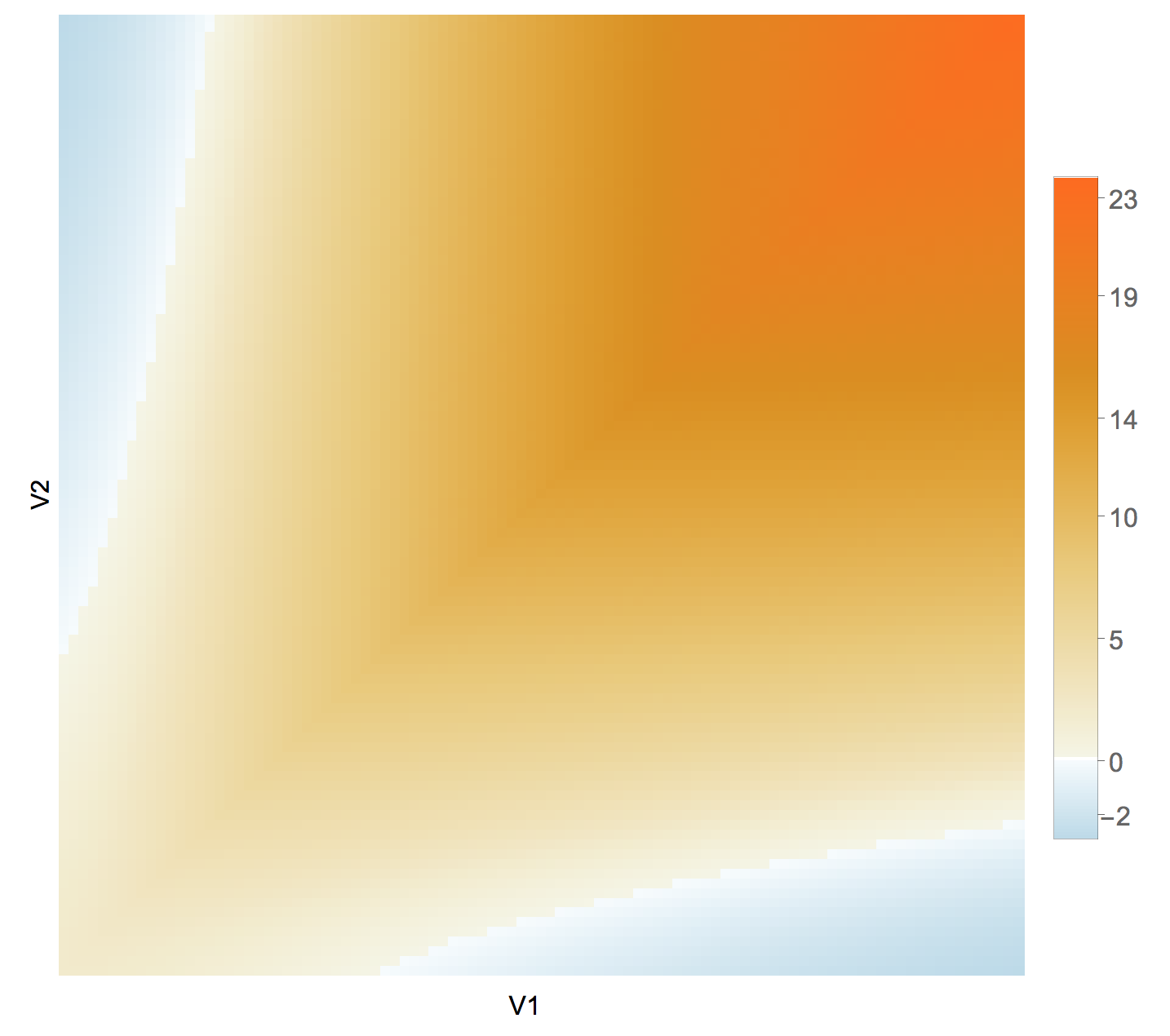
Definition 4.7.

For prescribed volumes $V_{1}\leq V_{2}$ , let

\mu(V_{1},V_{2})=P_{3}-P_{2}

be the difference between the perimeter $P_{3}$ of the triple interval and the perimeter $P_{2}$ of the double interval in equilibrium.

By Proposition 4.6, we obtain the following characterization.

(a)

If $\mu(V_{1},V_{2})<0$ , then the perimeter-minimizing double bubble is uniquely the triple interval.
(b)

If $\mu(V_{1},V_{2})>0$ , then the perimeter-minimizing double bubble is uniquely the double interval in equilibrium.
(c)

If $\mu(V_{1},V_{2})=0$ , then the perimeter-minimizing double bubble is either the triple interval or the double interval in equilibrium.

Let $f$ be a $C^{1}$ density. Observe that by equations (4) and (5), $\mu$ is a $C^{1}$ function with partial derivatives

	$\displaystyle\frac{\partial\mu}{\partial V_{1}}$	$\displaystyle=f^{\prime}\left(\frac{V_{1}}{2}\right)+f^{\prime}\left(\frac{V_{1}+V_{2}}{2}\right)+f^{\prime}(\widetilde{V}),$
	$\displaystyle\frac{\partial\mu}{\partial V_{2}}$	$\displaystyle=f^{\prime}\left(\frac{V_{1}+V_{2}}{2}\right)-f^{\prime}(\widetilde{V}+V_{1}+V_{2}).$

The remainder of this section investigates the behavior of $\mu$ .

Lemma 4.8.

On $\mathbb{R}$ with symmetric, strictly log-convex, $C^{1}$ density, for prescribed volumes $V_{1}<V_{2}$ ,

-\frac{V_{1}+V_{2}}{2}<\widetilde{V}<-V_{1}.

Proof.

Let $f$ be the density. Consider the equilibrium condition

f^{\prime}(\widetilde{V})+f^{\prime}(\widetilde{V}+V_{1})+f^{\prime}(\widetilde{V}+V_{1}+V_{2})=0.

By Lemma 4.2, $f$ is convex in volume coordinate, so the left-hand side is strictly increasing in $\widetilde{V}$ . At $\widetilde{V}=-(V_{1}+V_{2})/2$ , the left-hand side is negative, while at $\widetilde{V}=-V_{1}$ , the left-hand side is positive. Hence the value of $\widetilde{V}$ that makes the left-hand side vanish must lie inside the desired range. ∎

Lemma 4.9.

Consider $\mathbb{R}$ with symmetric, strictly log-convex, $C^{1}$ density. Given $V_{2}>0$ , $\mu$ is a strictly increasing function of $V_{1}\leq V_{2}$ . Given $V_{1}>0$ , $\mu$ is a strictly decreasing function of $V_{2}\geq V_{1}$ .

Proof.

Fix $V_{2}$ . For $V_{1}<V_{2}$ , we have

\frac{\partial\mu}{\partial V_{1}}=f^{\prime}\left(\frac{V_{1}}{2}\right)+f^{\prime}\left(\frac{V_{1}+V_{2}}{2}\right)+f^{\prime}(\widetilde{V})>f^{\prime}\left(\frac{V_{1}}{2}\right)>0

due to Lemma 4.8. Now fix $V_{1}$ . For $V_{2}>V_{1}$ , we have

\frac{\partial\mu}{\partial V_{2}}=f^{\prime}\left(\frac{V_{1}+V_{2}}{2}\right)-f^{\prime}(\widetilde{V}+V_{1}+V_{2})<0

due to Lemma 4.8. ∎

Proposition 4.10.

On $\mathbb{R}$ with symmetric, strictly log-convex, $C^{1}$ density, for equal prescribed volumes $V_{1}=V_{2}$ , we have $\mu>0$ (so the double interval is better).

Proof.

For $V_{1}=V_{2}$ , we have $\widetilde{V}=-V_{1}$ . So

P_{2}=2f(V_{1})+f(0)<2f\left(\frac{V_{1}}{2}\right)+2f(V_{1})=P_{3}.

∎

Proposition 4.11.

On $\mathbb{R}$ with symmetric, strictly log-convex, $C^{1}$ density $f$ such that $(\log f)^{\prime}$ is unbounded, given $V_{1}>0$ , we have $\mu<0$ for large $V_{2}\geq V_{1}$ (so the triple interval is better).

Proof.

Fix $V_{1}$ . For $V_{2}$ large, we need to show that

P_{2}=f(\widetilde{V})+f(\widetilde{V}+V_{1})+f(\widetilde{V}+V_{1}+V_{2})>2\left[f\left(\frac{V_{1}}{2}\right)+f\left(\frac{V_{1}+V_{2}}{2}\right)\right]=P_{3}.

By convexity of $f$ in volume coordinate (Lemma 4.2),

f(-\widetilde{V})+f(\widetilde{V}+V_{1}+V_{2})\geq 2f\left(\frac{V_{1}+V_{2}}{2}\right).

Notice that $f(-\widetilde{V})=f(\widetilde{V})$ by symmetry of $f$ . So we need to show that, for $V_{2}$ large,

f(\widetilde{V}+V_{1})>2f\left(\frac{V_{1}}{2}\right).

It suffices to show that $\widetilde{V}\to-\infty$ as $V_{2}\to\infty$ .

From the equilibrium condition

f^{\prime}(\widetilde{V})+f^{\prime}(\widetilde{V}+V_{1})+f^{\prime}(\widetilde{V}+V_{1}+V_{2})=0,

as $V_{2}\to\infty$ , if $\widetilde{V}$ does not become very small, then the leftmost two terms stay bounded, while the rightmost term goes to infinity because $f^{\prime}(V)$ is unbounded, which is a contradiction. Hence $\widetilde{V}\to-\infty$ as $V_{2}\to\infty$ . ∎

Remark 4.12.

Propositions 5.4 and 5.5 show that the hypothesis of strict log-convexity in Proposition 4.11 is necessary. Moreover, the following example shows that the hypothesis that $(\log f)^{\prime}$ is unbounded is needed.

Example 4.13.

Consider the density in volume coordinate $f(V)=\left\lvert V\right\rvert+e^{-\left\lvert V\right\rvert}$ . Notice that $f$ is $C^{1}$ and $f(V)$ is strictly convex, but $f^{\prime}(V)$ is bounded. For fixed $V_{1}$ , as $V_{2}\to\infty$ , it can be computed that $\widetilde{V}\to-\log(1+e^{V_{1}})$ . We can then check that

\mu\to 2V_{1}-\log(1+e^{V_{1}})+2e^{-V_{1}/2}-1>0

for all $V_{1}>0$ . Since $\mu$ is decreasing in $V_{2}$ (Lemma 4.9), $\mu>0$ and so the double interval is better for all $V_{1}$ and $V_{2}$ .

Lemma 4.14.

On $\mathbb{R}$ with symmetric, strictly log-convex, $C^{1}$ density, for small $V_{2}>0$ , $\mu>0$ for all $V_{1}\leq V_{2}$ (so the double interval is better).

Proof.

For $V_{2}$ small, by Lemma 4.8, $\widetilde{V}$ is also small in magnitude. Hence every density term that contributes to $P_{2}$ and $P_{3}$ is close to $f(0)$ . Thus for $V_{2}$ small, $P_{2}$ is close to $3f(0)$ while $P_{3}$ is close to $4f(0)$ , so that $P_{2}<P_{3}$ . ∎

Theorem 4.15.

On $\mathbb{R}$ with symmetric, strictly log-convex, $C^{1}$ density $f$ such that $(\log f)^{\prime}$ is unbounded, given $V_{1}>0$ , there is a unique $V_{2}=\lambda(V_{1})$ such that the double interval in equilibrium and the triple interval tie. For $V_{2}>\lambda(V_{1})$ , the perimeter-minimizing double bubble is uniquely the triple interval. For $V_{2}<\lambda(V_{1})$ , the perimeter-minimizing double bubble is uniquely the double interval in equilibrium. Moreover, $\lambda$ is a strictly increasing $C^{1}$ function that tends to a positive limit as $V_{1}\to 0$ .

Proof.

Fix $V_{1}$ . By Lemma 4.9, $\mu$ is a strictly decreasing function of $V_{2}$ . By Lemma 4.10, $\mu>0$ for $V_{2}=V_{1}$ . By Lemma 4.11, $\mu<0$ for large $V_{2}$ . These together imply that there is a unique $V_{2}=\lambda(V_{1})$ such that $\mu=0$ and that $\mu>0$ for $V_{2}<\lambda(V_{1})$ and $\mu<0$ for $V_{2}>\lambda(V_{1})$ . Thus $\lambda$ determines the perimeter-minimizing double bubbles as in the theorem statement.

Observe that $\mu$ is a $C^{1}$ function with partial derivative $\partial\mu/\partial V_{2}<0$ at points $(V_{1},\lambda(V_{1}))$ , by Lemma 4.9. So by the implicit function theorem, $\lambda$ is a $C^{1}$ function.

We now show that $\lambda$ is strictly increasing. Suppose not. Then there are $V_{1}<V_{1}^{*}$ with $\lambda(V_{1})\geq\lambda(V_{1}^{*})$ . By Lemma 4.9,

0=\mu(V_{1},\lambda(V_{1}))<\mu(V_{1}^{*},\lambda(V_{1}))\leq\mu(V_{1}^{*},\lambda(V_{1}^{*}))=0,

a contradiction. Note the term in the middle makes sense because $V_{1}^{*}\leq\lambda(V_{1})$ .

Finally we show that $\lambda$ tends to a positive limit as $V_{1}\to 0$ . By Lemma 4.14, there is $v>0$ such that $\mu>0$ for all $V_{1}\leq V_{2}\leq v$ , so $\lambda(V_{1})\neq v$ for all $V_{1}$ . Thus because $\lambda$ is strictly increasing, it tends to a limit which is at least as big as $v$ as $V_{1}\to 0$ . ∎

It is an interesting question what happens in the case where $(\log f)^{\prime}$ is bounded. In our follow-up note [So2], we show that the tie function $\lambda$ still exists but only for $V_{1}\in(0,V_{0})$ for some “blowup time” $0\leq V_{0}\leq\infty$ , and $\lambda\to\infty$ as $V_{1}\to V_{0}$ .

5. Non-Strictly Log-Convex Densities

Section 5 considers some densities which are symmetric, piecewise $C^{1}$ , and log-convex, but not strictly log-convex.

We investigate the following densities:

(i)

The constant density $f(x)=c$ (Prop. 5.4).
(ii)

The exponential density $f(x)=e^{\left\lvert x\right\rvert}$ (Prop. 5.5).

(iii)

The smoothed-out exponential density

(6)

f(x)=\begin{cases}e^{x^{2}}\quad&\text{for }\left\lvert x\right\rvert<a\\ e^{a(2\left\lvert x\right\rvert-a)}\quad&\text{for }\left\lvert x\right\rvert\geq a\end{cases}

with $a>2\sqrt{\log 2}$ (Prop. 5.9).

For the constant density, every double interval is perimeter minimizing. For the exponential density, a perimeter-minimizing double bubble is a double interval with the middle point at the origin. For the smoothed-out exponential density, the triple interval appears for $V_{1}$ small and $V_{2}$ large.

For non-strictly log-convex densities, there may be a continuum of double intervals (or triple intervals) in equilibrium with the prescribed volumes. Lemma 5.1 shows that all such are perimeter minimizing among double intervals (among triple intervals).

Lemma 5.1.

On $\mathbb{R}$ with symmetric log-convex density f, among n-bubbles of prescribed volumes and fixed combinatorial type, every equilibrium is perimeter minimizing.

Proof.

We may assume that $f$ is not constant, since the result is easy in that case. If we switch to volume coordinate (Lemma 4.2), then $f$ is a convex function of volume $V$ . Since $f$ is symmetric, convex, and nonconstant, it goes to infinity in both directions. Hence a minimizer exists. Since every minimizer is in equilibrium, it remains to show that every equilibrium has equal perimeter.

Represent an $n$ -bubble as a tuple of volume coordinates of endpoints of its components. Then given two $n$ -bubbles in equilibrium $B_{1}$ and $B_{2}$ , on the straight line between them, the volume of each component varies linearly. Since the volume of each bubble is equal at $B_{1}$ and $B_{2}$ , the volume of each bubble must be constant along this straight line. Hence all $n$ -bubbles along this straight line have the prescribed volumes. Let $P(t)$ denote the perimeter of the $n$ -bubble $(1-t)B_{1}+tB_{2}$ , $t\in[0,1]$ , on this straight line. Then $P$ is convex because $f$ is convex, and the one-sided derivatives $P^{\prime}_{R}(0)\geq 0$ and $P^{\prime}_{L}(1)\leq 0$ because $B_{1}$ and $B_{2}$ are in equilibria. It follows that $P$ is constant, and so $B_{1}$ and $B_{2}$ have equal perimeter. ∎

Remark 5.2.

Lemma 5.1 reduces the search for a perimeter-minimizing double bubble to any double interval or triple interval in equilibrium. We can pick a perimeter-minimizing triple interval to be the triple interval symmetric about the origin.

The proof shows that the set of (perimeter-minimizing) equilibria is a finite-dimensional cell, convex in the $V$ coordinates.

The hypothesis that $f$ be symmetric, used for the existence of a minimizer, is not necessary. If $f$ approaches but never reaches a limit in either direction, equilibria do not exist (because the derivative of perimeter is negative as you slide the $n$ -bubble in that direction), and the result holds trivially. Otherwise minimizers exist.

Remark 5.3.

By Lemma 5.1, in volume coordinates (Lemma 4.2), the perimeters $P_{2}$ of double and $P_{3}$ of triple intervals in equilibrium are still given by

	$\displaystyle P_{2}$	$\displaystyle=f(\widetilde{V})+f(\widetilde{V}+V_{1})+f(\widetilde{V}+V_{1}+V_{2}),$
	$\displaystyle P_{3}$	$\displaystyle=2\left[f\left(\frac{V_{1}}{2}\right)+f\left(\frac{V_{1}+V_{2}}{2}\right)\right],$

where $\widetilde{V}$ is any volume satisfying the equilibrium condition

f^{\prime}(\widetilde{V})+f^{\prime}(\widetilde{V}+V_{1})+f^{\prime}(\widetilde{V}+V_{1}+V_{2})=0.

We now consider some specific non-strict log-convex densities.

Proposition 5.4.

On $\mathbb{R}$ with density $f(x)=c$ , any double interval enclosing the prescribed volumes is perimeter minimizing.

Proof.

A double interval has perimeter $3c$ . Any other configuration has perimeter at least $4c$ . Therefore a double interval is perimeter minimizing. ∎

Proposition 5.5.

On $\mathbb{R}$ with density $f(x)=e^{\left\lvert x\right\rvert}$ , the perimeter-minimizing double bubble is the double interval with the middle perimeter point at the origin, unique up to reflection across the origin.

Proof.

The density in volume coordinate (Lemma 4.2) is

f(V)=1+\left\lvert V\right\rvert.

We first consider a double interval in equilibrium. The function $f$ is $C^{1}$ everywhere except at the origin with $f^{\prime}(V)=1$ or $-1$ . So the equilibrium condition (Rem. 5.3) cannot be satisfied unless one boundary point is at the origin. By Remark 3.4, the leftmost boundary point cannot be at the origin because the sum of the left derivatives

\sum f^{\prime}_{L}=1

would be positive. Similarly the rightmost boundary point cannot be at the origin. Hence the middle boundary point is at the origin. So the double interval in equilibrium is unique up to reflection across the origin.

Now we can compare the perimeters of double and triple intervals in equilibrium:

P_{2}=f(V_{1})+f(0)+f(V_{2})=V_{1}+V_{2}+3<2V_{1}+V_{2}+4=P_{3}.

Therefore the perimeter-minimizing double bubble is the double interval in equilibrium. ∎

We now consider the smoothed-out exponential density (6).

Lemma 5.6.

Consider $\mathbb{R}$ with the smoothed-out exponential density (6). Let $V_{1}\leq V_{2}$ be prescribed volumes. If

V_{1}+V_{2}\leq\int_{0}^{a}e^{x^{2}}\,dx,

then the perimeter-minimizing double bubbles are the same double and triple intervals as for the Borell density $f(x)=e^{x^{2}}$ of Proposition 4.6.

Proof.

By Proposition 3.5, a perimeter-minimizing double bubble consists of contiguous intervals. Observe that one of these intervals must contain the origin, as otherwise the whole double bubble can be shifted towards the origin and the perimeter will decrease. By the upper bound on $V_{1}+V_{2}$ , the whole bubble is contained in $[-a,a]$ . In this interval, the density is identical to the Borell density. By Proposition 4.6, a perimeter-minimizing double bubble for the Borell density also lies in this interval for the prescribed volumes. So perimeter-minimizing double bubbles for the two densities are identical. ∎

Lemma 5.7.

Consider $\mathbb{R}$ with the smoothed-out exponential density (6). Let $V_{1}\leq V_{2}$ be prescribed volumes, with

V_{1}\geq\int_{-a}^{a}e^{x^{2}}\,dx.

Then the double interval in equilibrium has the middle boundary point at the origin, and a triple interval in equilibrium has boundary points

-y_{2}<-y_{1}\leq-a<0<a\leq y_{1}^{\prime}<y_{2}^{\prime},

free up to the volume constraints.

Proof.

Observe that $f$ is $C^{1}$ and that

(\log f)^{\prime}(x)=\begin{cases}-2a\quad&\text{for }x\leq-a\\ 2x&\text{for }\left\lvert x\right\rvert<a\\ 2a&\text{for }x\geq a.\end{cases}

By Corollary 3.3, the sum of the derivatives of the log of the density at the boundary points of a double interval in equilibrium must equal zero. We claim that the middle boundary point is $0$ . If the middle boundary point were less than zero, then the sum of the derivatives of the log of the density would be negative. If the middle boundary point were greater than $0$ , then the sum of the derivatives of the log of the density would be positive. Therefore the middle boundary point is $0$ , as asserted.

For a triple interval in equilibrium, let the boundary points be $-y_{2}<-y_{1}<y_{1}^{\prime}<y_{2}^{\prime}$ . If $y_{1}^{\prime}$ is less than $a$ , then the sum of the derivatives of the log of the density at the boundary points is negative. If $-y_{1}$ is greater than $-a$ , then the sum of the derivatives of the log of the density at the boundary points is positive. Therefore $-y_{1}\leq-a<a\leq y_{1}^{\prime}$ , and the sum of the derivatives of the log of the density equals zero whenever this holds. So the claim holds. ∎

Lemma 5.8.

Consider $\mathbb{R}$ with the smoothed-out exponential density (6). Let $V_{1}\leq V_{2}$ be prescribed volumes, where

V_{1}<\int_{0}^{a}e^{x^{2}}\,dx,\quad V_{1}+V_{2}\geq\int_{-a}^{a}e^{x^{2}}\,dx.

Then a double interval in equilibrium has perimeter points $x_{1},x_{2},x_{3}$ , where

-a\leq x_{1}<x_{2}=-a-x_{1}\leq 0<a\leq x_{3},

up to reflection across the origin. A perimeter-minimizing triple interval has perimeter points

-y_{2}\leq-a<-y_{1}<0<y_{1}<a\leq y_{2}^{\prime},

where $[-y_{1},y_{1}]$ has volume $V_{1}$ and $y_{2}$ and $y_{2}^{\prime}$ are free up to the volume constraint.

Proof.

Let a double interval in equilibrium have boundary points $x_{1}<x_{2}<x_{3}$ , and assume that the left interval has volume $V_{1}$ . By Corollary 3.3,

(7)

(\log f)^{\prime}(x_{1})+(\log f)^{\prime}(x_{2})+(\log f)^{\prime}(x_{3})=0.

If $x_{1}<-a$ , then $x_{2}<0$ , and so (7) implies that $(\log f)^{\prime}(x_{3})>2a$ , which is impossible. Hence $x_{1}\geq-a$ . Because of the bound on $V_{1}+V_{2}$ , $x_{3}\geq a$ . Now by (7), $(\log f)^{\prime}(x_{2})\leq 0$ , so $x_{2}\leq 0$ . So (7) reduces to $x_{1}+x_{2}+a=0,$ or $x_{2}=-a-x_{1}$ . Then the inequality stated in the proposition holds. The resulting double interval is unique because there is only one $x_{1}$ such that $[x_{1},-a-x_{1}]$ has volume $V_{1}$ , and $x_{3}$ is determined from $x_{1}$ .

For a perimeter-minimizing triple interval, denote the boundary points by $-y_{2}<-y_{1}<y_{1}^{\prime}<y_{2}^{\prime}$ . By Corollary 3.3,

(8)		$\displaystyle(\log f)^{\prime}(-y_{1})+(\log f)^{\prime}(y_{1}^{\prime})$	$\displaystyle=0$
	$\displaystyle(\log f)^{\prime}(-y_{2})+(\log f)^{\prime}(y_{2}^{\prime})$	$\displaystyle=0,$

so either $-y_{2},y_{2}^{\prime}\in(-a,a)$ with $y_{2}=y_{2}^{\prime}$ or $-y_{2}\leq-a$ and $y_{2}^{\prime}\geq a$ . By the bound on $V_{1}+V_{2}$ , the latter must be the case. Similarly, either $-y_{1},y_{1}^{\prime}\in(-a,a)$ with $y_{1}=y_{1}^{\prime}$ or $-y_{1}\leq-a$ and $y_{1}^{\prime}\geq a$ . To determine which is the case, we must first determine whether $[-y_{1},y_{1}^{\prime}]$ encloses volume $V_{1}$ or $V_{2}$ .

We claim that $[-y_{1},y_{1}^{\prime}]$ must enclose volume $V_{1}$ . By the volume restriction on $V_{1}$ and (8), if $[-y_{1},y_{1}^{\prime}]$ has volume $V_{1}$ , then $-y_{1},y_{1}^{\prime}\in(-a,a)$ with $y_{1}=y_{1}^{\prime}$ . If $[-y_{1},y_{1}^{\prime}]$ encloses volume $V_{2}$ , then the magnitudes of $y_{1}$ and $y_{1}^{\prime}$ —and hence the perimeter $f(-y_{1})+f(y_{1}^{\prime})$ —will be greater than when $[-y_{1},y_{1}^{\prime}]$ encloses volume $V_{1}$ , so in order for the triple interval to be perimeter minimizing, $[-y_{1},y_{1}^{\prime}]$ must enclose volume $V_{1}$ . Then $y_{1}^{\prime}=y_{1}\in(0,a)$ , and therefore the boundary points satisfy the inequality in the statement of the proposition. ∎

The following proposition is our most interesting example, which shows that the appearance of the triple interval can depend on $V_{1}$ . The particular value $2\sqrt{\log 2}$ is just for our convenience.

Proposition 5.9.

Consider $\mathbb{R}$ with the smoothed-out exponential density (6):

f(x)=\begin{cases}e^{x^{2}}\quad&\text{for }\left\lvert x\right\rvert<a\\ e^{a(2\left\lvert x\right\rvert-a)}\quad&\text{for }\left\lvert x\right\rvert\geq a\end{cases}

with $a>2\sqrt{\log 2}$ . Let $V_{1}\leq V_{2}$ be prescribed volumes. If

(9)

V_{1}\geq\int_{-a}^{a}e^{x^{2}}\,dx,

then the perimeter-minimizing double bubble is the double interval in equilibrium for all $V_{2}$ (up to reflection). If $V_{1}$ is small, then for $V_{2}$ close to $V_{1}$ the perimeter-minimizing double bubble is the double interval in equilibrium and for $V_{2}$ large a perimeter-minimizing double bubble is a triple interval.

See Figure 10.

Proof.

By Proposition 3.5, a perimeter-minimizing double bubble consists of finitely many contiguous intervals. By Proposition 3.8, a perimeter-minimizing double bubble consists of two or three such intervals.

First consider the case when $V_{1}$ is small $V_{2}$ is close to $V_{1}$ . We assume that

V_{1}+V_{2}\leq\int_{0}^{a}e^{x^{2}}\,dx.

By Lemma 5.6, a perimeter-minimizing double bubble is identical to the one for the Borell density $f(x)=e^{x^{2}}$ with the same prescribed volumes. By Lemma 4.10, it is the double interval in equilibrium for $V_{2}$ close to $V_{1}$ .

Now suppose (9) holds. By Lemma 5.7, the boundary points of the double interval in equilibrium are $x_{1},0,x_{3}$ , where $x_{1}\leq-a$ and $x_{3}\geq a$ , and the boundary points of a triple interval in equilibrium are $-y_{2},-y_{1},y_{1}^{\prime},y_{2}^{\prime}$ , where we may choose $-y_{2}=x_{1}$ and hence $y_{2}^{\prime}=x_{3}$ . Thus we only need to compare the inner boundary points. Because $f(-y_{1})+f(y_{1}^{\prime})>f(0)=1$ , a double interval in equilibrium has less perimeter than a triple interval in equilibrium. Therefore the perimeter-minimizing double bubble is the double interval in equilibrium for all $V_{2}$ .

Finally, suppose that $V_{1}$ is small and $V_{2}$ is large. By Lemma 5.8, a double interval in equilibrium has boundary points $x_{1},x_{2},x_{3}$ , where $x_{2}$ is close to $-a/2$ , and a perimeter-minimizing triple interval has boundary points $-y_{2},-y_{1},y_{1},y_{2}^{\prime}$ , where $y_{1}$ is close to zero, $-y_{2}\leq-a$ , and $y_{2}^{\prime}\geq a$ . Observe that the single bubbles $[-y_{2},y_{2}^{\prime}]$ and $[x_{1},x_{3}]$ have volume $V_{1}+V_{2}$ and that by Corollary 3.3 the first single bubble is in equilibrium. Thus the perimeter of the outer boundary points of a perimeter-minimizing triple interval is less than or equal to the perimeter of the outer boundary points of a double interval in equilibrium. So it remains to examine the perimeter from the inner boundary points. Observe that

f\left(-\frac{a}{2}\right)=e^{{a^{2}}/4}>e^{(2\sqrt{\log 2})^{2}/4}=2=2f(0),

since $a>2\sqrt{\log 2}$ . Because $x_{2}$ is close to $-a/2$ and $y_{1}$ is close to 0, the perimeter from the inner boundary points of a perimeter-minimizing triple interval is less than the perimeter from the inner boundary points of a double interval in equilibrium. Then the total perimeter for a perimeter-minimizing triple interval is less than the total perimeter for a double interval in equilibrium. Therefore for $V_{1}$ small and $V_{2}$ large, a perimeter-minimizing double bubble is a triple interval. ∎

Conjecture 5.10.

Consider $\mathbb{R}$ with the smoothed-out exponential density (6). Let $V_{1}\leq V_{2}$ be prescribed volumes. Then there exists $V_{0}>0$ such that for $V_{1}\geq V_{0}$ , a perimeter-minimizing double bubble is always a double interval. For $0<V_{1}<V_{0}$ , there is a unique $V_{2}=\lambda(V_{1})$ such that double intervals and triple intervals tie. For $V_{2}>\lambda(V_{1})$ , a perimeter-minimizing double bubble is a triple interval. For $V_{2}<\lambda(V_{1})$ , a perimeter-minimizing double bubble is a double interval. Moreover, $\lambda$ is a strictly increasing $C^{1}$ function that tends to a positive limit as $V_{1}\to 0$ and tends to infinity as $V_{1}\to V_{0}$ .

6. Bounds on the Tie Points

We put some bounds on the growth of the function $V_{2}=\lambda(V_{1})$ , where the double and triple intervals tie, as defined in Theorem 4.15. From this point onwards we assume that $f$ is a symmetric, strictly log-convex, $C^{1}$ density such that $(\log f)^{\prime}$ is unbounded.

One of the main results of this section is that $\lambda(V_{1})/V_{1}\to\infty$ as $V_{1}\to\infty$ for densities $f=e^{\psi}$ such that $\psi_{xx}/\psi_{x}$ is bounded for $x$ large (Cor. 6.7). As in Remark 6.8, this implies that a line through the origin can intersect the tie curve $(V_{1},\lambda(V_{1}))$ more than once. For the Borell density, this is illustrated in Figure 4 of the Introduction.

Lemma 6.1.

For prescribed volumes $V_{1}\leq V_{2}$ , let $(x_{1},x_{2},x_{3})$ be the double interval in equilibrium (with the left interval enclosing volume $V_{1}$ ) and $(y_{1},y_{2})$ be the triple interval. Fix $V_{1}$ . As $V_{2}$ increases, $y_{2}$ and $x_{3}$ increase, while $x_{1}$ and $x_{2}$ decrease.

Proof.

It is easy to see that $y_{2}$ increases. As $V_{2}$ increases, $x_{3}$ can be moved to the right to accommodate the increased volume. The double interval is no longer in equilibrium, with

\sum_{i=1}^{3}\psi_{x}(x_{i})>0.

In order to be in equilibrium, the double interval must shift left. This implies that $x_{1}$ and $x_{2}$ decrease. To show that $x_{3}$ increases, note that in equilibrium,

\sum_{i=1}^{3}\psi_{x}(x_{i})=0.

So because $x_{1}$ and $x_{2}$ decrease, $x_{3}$ must increase so that the sum remains zero. ∎

The next lemma shows that the density in volume coordinate grows at least linearly but is approximately linear.

Lemma 6.2.

Let $f$ be a symmetric, strictly log-convex, $C^{1}$ density on $\mathbb{R}$ . In volume coordinate, there is $c>0$ such that for large $V$ ,

f(V)\geq cV.

Moreover,

\int_{0}^{\infty}\frac{1}{f(V)}

diverges.

In particular, this implies that although $f$ grows asymptotically at least as fast as $V$ , it cannot grow asymptotically faster than $V^{c}$ for any $c>1$ .

Proof.

Because $f^{\prime}$ is strictly increasing (Lemma 4.2), there is $\varepsilon>0$ such that for large $V$ , $f^{\prime}>\varepsilon$ . Hence for large $V$ , $f(V)\geq(\varepsilon/2)V$ .

The integral diverges because as we take $V\to\infty$ in the formula in Lemma 4.3, it must be the case that $x(V)\to\infty$ . ∎

The next lemma shows that the rate of growth of the volume of the interval $[0,x]$ is on the order of $f(x)/\psi_{x}$ for typical densities. Notice that the hypothesis $\psi_{x}^{2}\geq M\psi_{xx}$ for large $x$ is mild and holds for all densities we are interested in, namely $e^{x^{n}}$ and $e^{e^{x}}$ . In fact, it holds if the sign of $\psi_{x}^{2}-M\psi_{xx}$ changes only a finite number of times, because we can easily check that a function satisfying $\psi_{x}^{2}<M\psi_{xx}$ blows up in finite time.

Lemma 6.3 (Fundamental Bounding Lemma).

Let $f=e^{\psi}$ be a symmetric, strictly log-convex, $C^{1}$ density on $\mathbb{R}$ . For $x>0$ , define

V=\int_{0}^{x}f.

Then

\liminf_{x\to\infty}\frac{V}{f/\psi_{x}}\geq 1.

Furthermore, if $f$ is $C^{2}$ and $M>1$ is such that $\psi_{x}^{2}\geq M\psi_{xx}$ for $x$ large, then

\limsup_{x\to\infty}\frac{V}{f/\psi_{x}}\leq\frac{M}{M-1}.

In particular, if $\psi_{x}^{2}/\psi_{xx}\to\infty$ as $x\to\infty$ , then

\lim_{x\to\infty}\frac{V}{f/\psi_{x}}=1.

Proof.

In volume coordinate, we can rewrite the quatity in question via Lemma 4.2 as

\frac{V}{f/\psi_{x}}=\frac{V}{f(V)/f^{\prime}(V)}=\frac{Vf^{\prime}(V)}{f(V)}.

Because $f^{\prime}$ is nondecreasing,

f(V)-f(0)=\int_{0}^{V}f^{\prime}\leq Vf^{\prime}(V),

so that

\frac{Vf^{\prime}(V)}{f(V)}\geq\frac{f(V)-f(0)}{f(V)}\to 1

as $V\to\infty$ , implying the desired lower bound.

Now suppose $\psi_{x}^{2}\geq M\psi_{xx}$ for $x$ large. In volume coordinate, $\psi_{x}=f^{\prime}(V)$ and

\psi_{xx}=\frac{df^{\prime}(V)}{dx}=\frac{df^{\prime}(V)}{dV}\frac{dV}{dx}=f^{\prime\prime}(V)f(V).

So $f^{\prime 2}/(ff^{\prime\prime})\geq M$ for large $V$ . Now for $V$ large

\left(\frac{f}{f^{\prime}}\right)^{\prime}=\frac{f^{\prime 2}-ff^{\prime\prime}}{f^{\prime 2}}\geq 1-\frac{1}{M},

so that, for constants $c$ and $c_{1}$ ,

\frac{f}{f^{\prime}}=c+\int_{1}^{V}\left(\frac{f}{f^{\prime}}\right)^{\prime}\geq c_{1}+\frac{M-1}{M}V.

Therefore

\limsup_{V\to\infty}\frac{Vf^{\prime}}{f}\leq\frac{M}{M-1},

as desired. ∎

For lower bounds, we start by showing that, although $V_{2}^{*}\geq V_{1}$ by definition, it never approaches the line $V_{2}=V_{1}$ .

Proposition 6.4.

On $\mathbb{R}$ with a symmetric, strictly log-convex, $C^{1}$ density $f$ such that $(\log f)^{\prime}$ is unbounded, given $V_{1}>0$ , let $V_{2}^{*}$ be the unique value of $V_{2}$ such that the double interval in equilibrium and the triple interval tie. Then $V_{2}^{*}>2V_{1}$ for all $V_{1}>0$ .

Proof.

In volume coordinate (Lemma 4.2), we have

P_{2}=f(\widetilde{V})+f(\widetilde{V}+V_{1})+f(\widetilde{V}+V_{1}+V_{2}^{*})\\ =2f\left(\frac{V_{1}}{2}\right)+2f\left(\frac{V_{1}+V_{2}^{*}}{2}\right)=P_{3},

where $\widetilde{V}$ is the unique value such that the double interval is in equilibrium. If we use $-(V_{1}+V_{2}^{*})/2$ in place of $\widetilde{V}$ , then the resulting double interval has perimeter greater than or equal to the original perimeter:

P_{2}\leq 2f\left(\frac{V_{1}+V_{2}^{*}}{2}\right)+f\left(\frac{V_{2}^{*}-V_{1}}{2}\right).

Therefore

f\left(\frac{V_{2}^{*}-V_{1}}{2}\right)\geq 2f\left(\frac{V_{1}}{2}\right)>f\left(\frac{V_{1}}{2}\right),

so that, because $f$ is increasing, $V_{2}^{*}>2V_{1}$ . ∎

We now show that for slow-growing density $f$ , specifically where $Vf^{\prime\prime}(V)$ is bounded in volume coordinate, the function $\lambda$ grows superlinearly. We do not know whether this hypothesis is sharp.

Proposition 6.5.

Let $f$ be a symmetric, strictly log-convex, $C^{2}$ density on $\mathbb{R}$ . Suppose that, in volume coordinate, $f^{\prime}(V)$ is unbounded and $Vf^{\prime\prime}(V)$ is bounded. Given $V_{1}>0$ , let $V_{2}^{*}$ be the unique value of $V_{2}$ such that the double interval in equilibrium and the triple interval tie. Then $V_{2}^{*}/V_{1}\to\infty$ as $V_{1}\to\infty$ .

Proof.

By Lemma 6.2, there is $c>0$ such that for large $V_{1}$ , $2f(V_{1}/2)>2cV_{1}>cV_{1}+f(0)$ . So

		$\displaystyle cV_{1}\leq 2f\left(\frac{V_{1}}{2}\right)-f(0)=\mu(V_{1},V_{1})-\mu(V_{1},V_{2}^{*})$
		$\displaystyle=-\int_{V_{1}}^{V_{2}^{}}\frac{\partial\mu}{\partial V_{2}}\,dV_{2}=\int_{V_{1}}^{V_{2}^{}}f^{\prime}(\widetilde{V}+V_{1}+V_{2})-f^{\prime}\left(\frac{V_{1}+V_{2}}{2}\right)\,dV_{2}$
		$\displaystyle\leq\int_{V_{1}}^{V_{2}^{}}f^{\prime}(V_{2})-f^{\prime}(V_{1})\,dV_{2}\leq\int_{V_{1}}^{V_{2}^{}}f^{\prime}(V_{2}^{*})-f^{\prime}(V_{1})\,dV_{2}$
		$\displaystyle=(V_{2}^{}-V_{1})(f^{\prime}(V_{2}^{})-f^{\prime}(V_{1}))\leq V_{2}^{}(f^{\prime}(V_{2}^{})-f^{\prime}(V_{1})),$

where the third line follows because $f^{\prime}$ is nondecreasing and $\widetilde{V}<-V_{1}$ due to Lemma 4.8. Therefore, for $V_{1}$ large,

(10)

f^{\prime}(V_{2}^{*})-f^{\prime}(V_{1})\geq\frac{c}{V_{2}^{*}/V_{1}}.

Because $f^{\prime}$ is unbounded, $f(V)/V\to\infty$ as $V\to\infty$ , and so the constant $c$ in (10) can be taken arbitrarily large. By hypothesis on the growth of $f$ , there is $c_{1}>0$ such that $f^{\prime\prime}(V)\leq c_{1}/V$ . So

f^{\prime}(V_{2}^{*})-f^{\prime}(V_{1})=\int_{V_{1}}^{V_{2}^{*}}f^{\prime\prime}\leq c_{1}\int_{V_{1}}^{V_{2}^{*}}\frac{1}{V}=c_{1}\log\frac{V_{2}^{*}}{V_{1}}.

Hence by (10)

\frac{V_{2}^{*}}{V_{1}}\log\frac{V_{2}^{*}}{V_{1}}\geq\frac{c}{c_{1}}.

As $V_{1}\to\infty$ , $c$ can be taken arbitrarily large, and so $V_{2}^{*}/V_{1}\to\infty$ , as desired. ∎

Remark 6.6.

Instead of $f$ being $C^{2}$ , it suffices to assume that $f$ is $C^{1}$ and that there is $c>0$ such that $f^{\prime}(V)-c\log V$ is eventually nonincreasing.

The following corollary translates the hypothesis of Proposition 6.5 to the positional coordinate. It says that the conclusion of Proposition 6.5 holds for well-behaved densities that can grow as fast as $\exp(e^{cx})$ , because this is the density where $\psi_{xx}/\psi_{x}$ is constant. We do not know whether this condition is sharp.

Corollary 6.7.

Let $f=e^{\psi}$ be a symmetric, strictly log-convex, $C^{2}$ density on $\mathbb{R}$ , where $\psi_{x}$ is unbounded and $\psi_{xx}/\psi_{x}$ is bounded for $x$ large. Given $V_{1}>0$ , let $V_{2}^{*}$ be the unique value of $V_{2}$ such that the double interval in equilibrium and the triple interval tie. Then $V_{2}^{*}/V_{1}\to\infty$ as $V_{1}\to\infty$ .

Moreover, there is $c>0$ such that for any $\varepsilon>0$ , for $V_{1}$ large,

V_{2}^{*}\geq V_{1}(\psi_{x}f^{-1}(cV_{1}))^{1-\varepsilon},

where $f^{-1}$ is the inverse function of the density in the positional coordinate.

Proof.

Because $\psi_{x}$ is unbounded and $\psi_{xx}/\psi_{x}$ is bounded for $x$ large, $\psi_{x}^{2}/\psi_{xx}\to\infty$ as $x\to\infty$ , so the Fundamental Bounding Lemma 6.3 applies. We have

Vf^{\prime\prime}(V)=V\frac{df^{\prime}(V)}{dV}=V\frac{d\psi_{x}}{dx}\frac{dx}{dV}=\frac{V\psi_{xx}}{f}.

By Lemma 6.3, $V$ is on the same order as $f/\psi_{x}$ for $x$ large, so $Vf^{\prime\prime}(V)$ is on the same order as $\psi_{xx}/\psi_{x}$ , which is bounded. Therefore the conclusion of the first part follows from Proposition 6.5.

For the second part, we use the method of Proposition 6.5 to arrive at

(11)

\frac{V_{2}^{*}}{V_{1}}\log\frac{V_{2}^{*}}{V_{1}}\geq c\frac{f(V_{1}/2)}{V_{1}}

for some constant $c>0$ . By Lemma 6.3, the quantity on the right-hand side is on the same order as $\psi_{x}(x(V_{1}/2))$ , where $x$ is the function that converts from volume to positional coordinate. By Lemma 6.2, there is a constant $c_{1}>0$ such that

f(x(V))\geq c_{1}V

for $V$ large. Because $f$ is strictly increasing,

x(V)\geq f^{-1}(c_{1}V).

So (11) becomes

\frac{V_{2}^{*}}{V_{1}}\log\frac{V_{2}^{*}}{V_{1}}\geq c\psi_{x}f^{-1}(c_{1}V/2),

which implies the conclusion. ∎

Remark 6.8.

Along a line $V_{2}=rV_{1}$ , the perimeter minimizer may change from a triple interval to a double interval and back to a triple interval, as numerically plotted for the Borell density $f(r)=\exp\left(r^{2}\right)$ in Figure 4 of the introduction, where the line $V_{2}=10V_{1}$ intersects the curve of tie points in two places. Indeed, whenever $\psi_{x}$ is unbounded and $\psi_{xx}/\psi_{x}$ is bounded for $x$ large, Corollary 6.7 implies that $\lambda(V_{1})/V_{1}\to\infty$ as $V_{1}\to\infty$ , while by Theorem 4.15, $\lambda$ tends to a positive limit as $V_{1}\to 0$ , so $\lambda(V_{1})/V_{1}\to\infty$ as $V_{1}\to 0$ . Thus $\lambda(V_{1})/V_{1}$ must assume some value twice in the interval $(0,\infty)$ .

The next two corollaries follow immediately from Corollary 6.7. Corollary 6.9 gives a lower bound on the tie function $\lambda$ for the Borell density. Numerics suggest that the bound is not sharp: Figure 4 of the introduction suggests that $\lambda$ grows approximately quadratically for the Borell density.

Corollary 6.9.

On $\mathbb{R}$ with the Borell density $f(x)=e^{x^{2}}$ , given $V_{1}>0$ , let $V_{2}^{*}$ be the unique value of $V_{2}$ such that the double interval in equilibrium and the triple interval tie. Then for all $\varepsilon>0$ ,

V_{2}^{*}\geq V_{1}(\log V_{1})^{1/2-\varepsilon}

for $V_{1}$ large.

Corollary 6.10.

On $\mathbb{R}$ with the density $f(x)=e^{e^{x}}$ , given $V_{1}>0$ , let $V_{2}^{*}$ be the unique value of $V_{2}$ such that the double interval in equilibrium and the triple interval tie. Then for all $\varepsilon>0$ ,

V_{2}^{*}\geq V_{1}(\log V_{1})^{1-\varepsilon}

for $V_{1}$ large.

The following proposition gives an upper bound for the tie points. Note that the hypothesis $\psi^{2}\geq M\psi_{x}$ for $x$ large is mild. In fact, $\psi^{2}<M\psi_{x}$ cannot hold for all $x$ large, since this inequality implies that the $\psi$ blows up in finite time.

Proposition 6.11.

Let $f=e^{\psi}$ be a symmetric, strictly log-convex, $C^{1}$ density on $\mathbb{R}$ , where $\psi_{x}$ is unbounded and $\psi^{2}\geq M\psi_{x}$ for $x$ large. Given $V_{1}>0$ , let $V_{2}^{*}$ be the unique value of $V_{2}$ such that the double interval in equilibrium and the triple interval tie. Then, for constants $c_{1}>0$ and $c_{2}$ ,

V_{2}^{*}\leq c_{1}\exp\left(\psi\psi_{x}^{-1}(2\psi_{x}A)\right)

for $V_{1}$ large, where

A=\psi^{-1}(\log V_{1}+2\log\log V_{1}+c_{2}).

Proof.

Let $V_{2}=V_{2}^{*}$ . Let the double interval in equilibrium be $(x_{1},x_{2},x_{3})$ and the triple interval be $(y_{1},y_{2})$ . We have

f(x_{1})+f(x_{2})+f(x_{3})=P_{3}=P_{2}=2f(y_{1})+2f(y_{2}).

By Proposition 3.6, the interval $[-y_{2},y_{2}]$ is the best single bubble for volume $V_{1}+V_{2}$ , so

f(x_{1})+f(x_{3})\geq 2f(y_{2}).

Thus

f(x_{2})\leq 2f(y_{1}),

which is equivalent to

(12)

\psi(x_{2})\leq\psi(y_{1})+\log 2.

By the Fundamental Bounding Lemma 6.3, for $x$ large,

(13)

f(x)\leq 2V(x)\psi_{x}(x)\leq\frac{2}{M}V(x)\psi(x)^{2}=\frac{2}{M}V(x)(\log f)^{2},

because $\psi^{2}\geq M\psi_{x}$ for $x$ large. For $x$ large, $\log f\leq f^{1/4}$ , so (13) implies that $f\leq cV^{2}$ for a constant $c$ . Using this on the right-hand side of (13) gives $f\leq cV(\log V)^{2}$ for a new constant $c$ (we allow $c$ to change from line to line). Hence (12) becomes

	$\displaystyle\psi(x_{2})$	$\displaystyle\leq\log f(y_{1})+\log 2\leq\log V(y_{1})+2\log\log V(y_{1})+c$
(14)			$\displaystyle\leq\log V_{1}+2\log\log V_{1}+c,$

because $V(y_{1})=V_{1}/2$ . So $\left\lvert x_{2}\right\rvert\leq A$ , where $A$ is defined as in the proposition statement.

We now estimate $x_{1}$ . We have

V_{1}=\int_{|x_{2}|}^{|x_{1}|}f\geq\frac{1}{\psi_{x}(|x_{1}|)}\int_{|x_{2}|}^{|x_{1}|}\psi_{x}f=\frac{f(x_{1})-f(x_{2})}{\psi_{x}(|x_{1}|)}.

	$\displaystyle f(x_{1})$	$\displaystyle\leq f(x_{2})+\psi_{x}(\|x_{1}\|)V_{1}\leq f(x_{2})+\frac{1}{M}\psi(x_{1})^{2}V_{1}$
		$\displaystyle=f(x_{2})+\frac{1}{M}(\log f(x_{1}))^{2}V_{1}$
(15)			$\displaystyle\leq cV_{1}(\log V_{1})^{2}+\frac{1}{M}(\log f(x_{1}))^{2}V_{1},$

by (14). For $x$ large, $\log f\leq f^{1/4}$ , so by (15),

f(x_{1})\leq cV_{1}(\log V_{1})^{2}+\frac{1}{M}f(x_{1})^{1/2}V_{1}.

Solving gives $f(x_{1})\leq cV_{1}^{2}$ . Applying this to the right-hand side of (15) yields

f(x_{1})\leq cV_{1}(\log V_{1})^{2}.

Hence

(16)

\psi(x_{1})=\log f(x_{1})\leq\log V_{1}+2\log\log V_{1}+c,

which implies that $\left\lvert x_{1}\right\rvert\leq A$ where $A$ is defined as in the proposition statement.

Therefore, for $V_{1}$ large,

	$\displaystyle V_{2}^{*}$	$\displaystyle\leq 2\int_{0}^{x_{3}}f\leq 2\int_{1}^{x_{3}}f\leq\frac{2}{\psi_{x}(1)}\int_{1}^{x_{3}}\psi_{x}f$
		$\displaystyle=\frac{2(f(x_{3})-f(1))}{\psi_{x}(1)}\leq cf(x_{3})=c\exp\psi(x_{3})$
		$\displaystyle=\exp\psi\psi_{x}^{-1}(\psi_{x}(x_{3}))=\exp\psi\psi_{x}^{-1}\left(\psi_{x}(\|x_{1}\|)+\psi_{x}(\|x_{2}\|)\right)$
		$\displaystyle\leq\exp\psi\psi_{x}^{-1}(2\psi_{x}A),$

by (14) and (16), because $f^{\prime}=f\psi_{x}$ and $\psi_{x}(x_{3})=\psi_{x}(|x_{1}|)+\psi_{x}(|x_{2}|)$ due to the equilibrium. ∎

The following corollaries compute the upper bounds explicitly for the densities $e^{x^{2}}$ and $e^{e^{x}}$ .

Corollary 6.12.

V_{2}^{*}\leq V_{1}^{4+\varepsilon}

for $V_{1}$ large.

Proof.

Since $\psi=x^{2}$ and $\psi_{x}=2x$ , $\psi^{2}\geq\psi_{x}$ for $x$ large, so Proposition 6.11 applies. Therefore

	$\displaystyle V_{2}^{*}$	$\displaystyle\leq c_{1}\exp{4(\log V_{1}+2\log\log V_{1}+c_{2})}$
		$\displaystyle=cV_{1}^{4}(\log V_{1})^{8}\leq V_{1}^{4+\varepsilon}$

for any $\varepsilon>0$ and $V_{1}$ large, where $c_{1}$ , $c_{2}$ and $c$ are constants. ∎

Corollary 6.13.

V_{2}^{*}\leq V_{1}^{2+\varepsilon}

for $V_{1}$ large.

Proof.

Since $\psi=\psi_{x}=e^{x}$ , $\psi^{2}\geq\psi_{x}$ for $x$ large, so Proposition 6.11 applies. Therefore

	$\displaystyle V_{2}^{*}$	$\displaystyle\leq c_{1}\exp{2(\log V_{1}+2\log\log V_{1}+c_{2})}$
		$\displaystyle=cV_{1}^{2}(\log V_{1})^{4}\leq cV_{1}^{2+\varepsilon}$

for any $\varepsilon>0$ and $V_{1}$ large, where $c_{1}$ , $c_{2}$ and $c$ are constants. ∎

7. Higher Dimensions

In $\mathbb{R}^{N}$ with radial density going to infinity, for any $n$ given volumes, a perimeter-minimizing $n$ -bubble exists by an argument ([BDKS], Rmk. 3.3) after Morgan and Pratelli ([MP], Thm. 3.3).

In this section we use numerical techniques to determine the shape and surface area of potentially perimeter-minimizing double bubbles in higher dimensions with Borell density $e^{r^{2}}$ as in Figure 3 of the Introduction. The code used for these computations can be found at https://github.com/arjunkakkar8/doublebubble.

To do so, we use the software Brakke’s Surface Evolver [Br]. Starting with an initial shape, the surface evolver iteratively minimizes the energy associated with that configuration by moving its pieces while maintaining the values of constraints defined on the configuration.

To examine the double bubble in space with Borell density, we define the initial configuration of two adjacent cubes (squares in the plane). Then the energy of the system is defined as the weighted perimeter of the cubes. Next the weighted volume of the cubes is calculated by using the divergence theorem. With boundary $B$ , the weighted volume is

V_{B}=\oint_{B}\mathbf{F}\cdot\mathbf{n},\text{ where }\nabla\cdot\mathbf{F}=e^{\mathbf{r}^{2}}.

Note that the choice of $\mathbf{F}$ for which $\nabla\cdot\mathbf{F}=e^{\mathbf{r}^{2}}$ is not unique. We used ?

\mathbf{F}=\bigg(e^{y^{2}+z^{2}}\int e^{x^{2}}dx,\quad 0,\quad 0\bigg).

Since there is no closed form for the integral, the vector field is evaluated by using a series expansion. Care is taken to use sufficiently many terms so that within the relevant radius, the error from the approximation is negligible compared to the 4-digit precision of the Evolver. Then the system is evolved down the energy gradient while fixing the weighted volumes. The final state that the system converges to for the case of 2D and of 3D is depicted in Figure 3.

In closing, we conjecture that some of the behavior on $\mathbb{R}^{1}$ will recur in higher dimensions.

Conjecture 7.1.

In $\mathbb{R}^{N}$ with a smooth, radial, log-convex density, a perimeter-minimizing double bubble is either

(i)

the bubble inside a bubble (e.g. for $V_{1}$ small and $V_{2}$ large), or
(ii)

the standard double bubble (e.g. for $V_{2}$ close to $V_{1}$ ).

References

Ba [Ba] V. Bayle (2004). Propriétés de concavité du profil isopérimétrique et applications, PhD thesis, Institut Joseph Fourier, Grenoble.
BDKS [BDKS] Eliot Bongiovanni, Alejandro Diaz, Arjun Kakkar, Nat Sothanaphan. Isoperimetry in surfaces of revolution with density, Missouri J. Math. Sci. 30 (2018), no. 2, 150–165. https://arxiv.org/abs/1709.06040.
Br [Br] Kenneth Brakke. The surface evolver, http://facstaff.susqu.edu/brakke/evolver/evolver.html.
BH [BH] Serguei G. Bobkov, Christian Houdré (1997). Some connections between isoperimetric and Sobolev-type inequalities, Mem. Amer. Math. Soc. 129, no. 616, viii+111.
Ch [Ch] Gregory R. Chambers (2015). Proof of the Log-Convex Density Conjecture. J. Eur. Math. Soc., to appear.
M [M] Frank Morgan (2016). Geometric Measure Theory: A Beginner’s Guide, Academic press.
MN [MN] Emanuel Milman, Joe Neeman (2018). The Gaussian double-bubble conjecture, preprint. https://arxiv.org/abs/1801.09296.
MP [MP] Frank Morgan, Aldo Pratelli (2013). Existence of isoperimetric regions in $\mathbb{R}^{n}$ with density, Ann. Glob. Anal. Geom. 43, 331-365.
MG [MG] Ivor McGillivray (2017). An isoperimetric inequality in the plane with a log-convex density, preprint. https://arxiv.org/abs/1612.07052.
RCBM [RCBM] César Rosales, Antonio Cañete, Vincent Bayle, Frank Morgan (2008). On the isoperimetric problem in Euclidean space with density, Calc. Var. 31, 27-46.
So1 [So1] Nat Sothanaphan (2018). 1D Triple Bubble Problem with Log-Convex Density. https://arxiv.org/abs/1805.08377.
So2 [So2] Nat Sothanaphan. Double Bubbles on the Line with Log-convex Density $f$ with $(\log f)^{\prime}$ Bounded, Missouri J. Math. Sci. 30 (2018), no. 2, 166–175. https://arxiv.org/abs/1807.02661.

Eliot Bongiovanni
Michigan State University
eliotbonge@gmail.com

Leonardo Di Giosia
Rice University
lsd2@rice.edu

Alejandro Diaz
University of Maryland, College Park
diaza5252@gmail.com

Jahangir Habib
Williams College
jih1@williams.edu

Arjun Kakkar
Williams College
ak23@williams.edu

Lea Kenigsberg
Columbia University in the City of New York
lk2720@columbia.edu

Dylanger Pittman
Williams College
dsp1@williams.edu

Nat Sothanaphan
Massachusetts Institute of Technology
natsothanaphan@gmail.com

Weitao Zhu
Williams College
wz1@williams.edu

		$\displaystyle cV_{1}\leq 2f\left(\frac{V_{1}}{2}\right)-f(0)=\mu(V_{1},V_{1})-\mu(V_{1},V_{2}^{*})$
		$\displaystyle=-\int_{V_{1}}^{V_{2}^{}}\frac{\partial\mu}{\partial V_{2}}\,dV_{2}=\int_{V_{1}}^{V_{2}^{}}f^{\prime}(\widetilde{V}+V_{1}+V_{2})-f^{\prime}\left(\frac{V_{1}+V_{2}}{2}\right)\,dV_{2}$
		$\displaystyle\leq\int_{V_{1}}^{V_{2}^{}}f^{\prime}(V_{2})-f^{\prime}(V_{1})\,dV_{2}\leq\int_{V_{1}}^{V_{2}^{}}f^{\prime}(V_{2}^{*})-f^{\prime}(V_{1})\,dV_{2}$
		$\displaystyle=(V_{2}^{}-V_{1})(f^{\prime}(V_{2}^{})-f^{\prime}(V_{1}))\leq V_{2}^{}(f^{\prime}(V_{2}^{})-f^{\prime}(V_{1})),$

Double Bubbles on the Real Line with Log-Convex Density

Abstract.

1. Introduction

Proposition 1.1 (Prop. 4.10).

Proposition 1.2 (Prop. 4.11).

Theorem 1.3 (Thm. 4.15).

Outline of proofs

Outline of paper

Acknowledgements

2. Densities and Bubbles

Definition 2.1.

3. nn-Bubbles on the Real Line

Proposition 3.1.

Proof.

Proposition 3.2.

Proof.

Corollary 3.3.

Proof.

Remark 3.4.

Proposition 3.5.

Proof.

Proposition 3.6 (Single bubble).

Proof.

Lemma 3.7.

Proof.

Proposition 3.8.

Proof.

Remark 3.9.

4. Double Bubbles on the Real Line

Definition 4.1.

Lemma 4.2 (Volume coordinate).

Proof.

Lemma 4.3.

Proof.

Lemma 4.4.

Proof.

Lemma 4.5.

Proof.

Proposition 4.6.

Volume and perimeter relationships

Characterizations of when the double or triple interval is perimeter minimizing

Definition 4.7.

Lemma 4.8.

Proof.

Lemma 4.9.

Proof.

Proposition 4.10.

Proof.

Proposition 4.11.

Proof.

Remark 4.12.

Example 4.13.

Lemma 4.14.

Proof.

Theorem 4.15.

Proof.

5. Non-Strictly Log-Convex Densities

Lemma 5.1.

Proof.

Remark 5.2.

Remark 5.3.

Proposition 5.4.

Proof.

Proposition 5.5.

Proof.

Lemma 5.6.

Proof.

Lemma 5.7.

Proof.

Lemma 5.8.

Proof.

Proposition 5.9.

Proof.

Conjecture 5.10.

6. Bounds on the Tie Points

Lemma 6.1.

Proof.

Lemma 6.2.

Proof.

Lemma 6.3 (Fundamental Bounding Lemma).

3. $n$ -Bubbles on the Real Line