Final Thoughts on the Power Spectra of Scalar Potential Models
D. J. Brooker1∗, N. C. Tsamis2+ and R. P. Woodard1†
1 Department of Physics, University of Florida,
Gainesville, FL 32611, UNITED STATES
2 Institute of Theoretical Physics & Computational Physics,
Department of Physics, University of Crete,
GR-710 03 Heraklion, HELLAS
ABSTRACT
We give final shape to a recent formalism for deriving the functional
forms of the primordial power spectra of single-scalar potential models
and theories which are related to them by conformal transformation. An
excellent analytic approximation is derived for the nonlocal correction
factors which are crucial to capture the “ringing” that can result from
features in the potential. We also present the full algorithm for using
our representation, including the nonlocal factors, to reconstruct the
inflationary geometry from the power spectra.
PACS numbers: 04.50.Kd, 95.35.+d, 98.62.-g
∗ e-mail: djbrooker@ufl.edu
+ e-mail: tsamis@physics.uoc.gr
† e-mail: woodard@phys.ufl.edu
1 Introduction
The simplest models of primordial inflation are based on general relativity
(for a spacelike metric ) plus a single, minimally coupled
scalar ,
(1)
A key prediction is the generation of tensor [1] and
scalar [2] perturbations. These are the first observable
quantum gravitational phenomena ever recognized as such [3, 4, 5]. They are also our chief means of
testing the viability of scalar potential models [6, 7, 8], and of reconstructing
[9, 10, 11].
Reconstruction is simplest in terms of the Hubble representation
[12] using the Hubble parameter and first slow roll
parameter of the homogeneous, isotropic and spatially flat
background geometry of inflation,111
The connection to the potential
representation is [13, 14, 15, 16, 17],
(2)
Let stand for the time of first horizon crossing, when modes of wave
number obey . The tensor and scalar power spectra
take the form of leading slow roll results at , multiplied by local
slow roll corrections also at , times nonlocal factors involving times
near [18, 19],
(3)
(4)
The local slow roll correction is,
(5)
The nonlocal correction exponents, and ,
vanish for and effectively depend on the geometry only a few
e-foldings before and after [18, 19].
The purpose of this paper is to rationalize and simplify our formalism for
evolving the norms of the mode functions, rather than the mode functions
[20], and then to derive an excellent analytic approximation
for the nonlocal correction exponents and .
We also demonstrate how this approximation can be used to reconstruct the
inflationary geometry from the power spectra, even for models which possess
features. These topics represent sections 2-3, 4 and 5, respectively. In section
6 we discuss some of the many applications [21, 22]
this formalism facilitates.
Figure 1: The left hand graph shows one model’s scalar power spectrum as a
function of , the number of e-foldings from the beginning of inflation
to first horizon crossing. The right hand graph shows the same power spectrum
versus , the number of e-foldings until the end of inflation. Early
times correspond to small and large , whereas late times correspond to
large and small .
We shall often employ the alternate time parameter provided by , the number of e-foldings since inflation’s onset. This is
superior to the co-moving time by virtue of being dimensionless and
relating evolution to the size of the universe. We shall abuse the notation
slightly by writing and , instead of the correct but
cumbersome expressions and . Which time parameter
pertains should be clear from context, and from our exclusive use of ,
and to stand for e-foldings. Over-dots represent time derivatives
and primes stand for derivatives,
(6)
We caution readers against confusing with the common parameter , the number of e-foldings until the end of inflation (at ).
Figure 1 illustrates the difference.
2 Our Formalism in General
The tree order tensor power spectrum is obtained by evolving the graviton
mode function past the time of first horizon crossing
[9, 10, 11],
(7)
We do not possess exact solutions for for realistic geometries
, but we do know the evolution equation, the Wronskian and the
form at asymptotically early times [9, 10, 11, 23],
(8)
Because the power spectrum depends upon the norm-squared, rather than the
rapidly-varying phase, it is better to convert (8) into a
nonlinear evolution equation for
[20],
(9)
If necessary, the mode function can be easily recovered [19],
(10)
Relation (9) can be improved by changing to the dimensionless
time parameter ,
(11)
A further improvement comes by factoring out an (at this stage) arbitrary
approximate solution, , to derive a damped, driven oscillator
equation (with small nonlinearities) for the residual exponent
[18],
(12)
Here the frequency and the tensor source are,
(13)
It is an amazing fact that an exact Green’s function exists for the
left hand side of equation (12), valid for any choice of the
approximate solution [18],
(14)
This permits us to solve (12) perturbatively
by expanding in the nonlinear terms,
(15)
(16)
The tree order scalar power spectrum is obtained by evolving the
mode function past the time of first horizon crossing
[9, 10, 11],
(17)
Just as for its tensor cousin, we lack exact solutions for for realistic
geometries , but we do know the evolution equation, the Wronskian
and the form at asymptotically early times [9, 10, 11, 23],
The scalar mode function mode can be recovered from
[19],
(20)
Converting from co-moving time to gives,
(21)
Factoring out by an arbitrary approximate solution
produces another damped, driven oscillator equation for the residual exponent,
(22)
Here the frequency and the scalar source are,
(23)
(24)
Making the replacement in (14) gives
an exact Green’s function which is valid for any choice of ,
(25)
And we can of course develop a perturbative solution to (22)
,
(26)
(27)
3 Choosing and Effectively
The formalism of the previous section is valid for all choices of the approximate
solutions and . Of course the correction exponents
and will be smaller if the zeroth order solutions are more
carefully chosen. In previous work we used the instantaneously constant
solutions [18, 19],
(28)
where we define,
(29)
However, the choice (28) has the undesirable effect of complicating the
late time limits. The physical quantities and freeze
in to constant values soon after first horizon crossing, but continued evolution
in prevents and from approaching
constants. Hence the residual exponents and must evolve so as
to cancel this effect.
We can make the late time limits simpler by adopting a piecewise choice for the
approximate solutions,
(30)
(31)
By and we mean the
solutions which would pertain for the ersatz geometry,
(32)
Here and henceforth stands for the number of e-foldings
from horizon crossing. To be explicit about the over-lined quantities,
(33)
With the choice (30-31) the approximate solutions rapidly
freeze in to constants,
(34)
This establishes the forms (3-4) for the power spectra and
fixes the nonlocal correction exponents to,
(35)
It remains to specialize the sources to (30-31). First
note the simple relation between the scalar and tensor frequencies,
(36)
This means the scalar source (24) consists of the tensor source
(13) minus a handful of terms mostly involving ,
(37)
To obtain an explicit formula for the tensor source we first note that the
tensor frequency is,
(38)
Hence the derivative of its logarithm is,
(39)
where and . Before horizon crossing
is time dependent and so we have,
(40)
where and involve derivatives of
with respect to and ,
(41)
The analogous result after horizon crossing is much simpler,
(42)
where means with specialized to
and specialized to .
Taking the derivative of before horizon crossing,
(43)
requires three second derivatives of ,
(44)
Bessel’s equation and the Wronskian of imply,
(45)
Substituting relations (39), (40), (43) and
(45) in the definition of the tensor source (13)
gives,
(46)
The analogous result after horizon crossing is,
(47)
There is also a jump at horizon crossing so that the complete result is,
(48)
Figure 2: The left hand graph shows the local slow roll correction factor
(solid blue), which was defined inexpression (5). Also
shown is its global approximation of (dashed yellow) over the
full inflationary range of . The right hand graph shows
(solid blue) versus the better approximation of
(large dots) relevant to the range favored by current
data.
4 Simple Analytic Approximations
The exact analytic results of the previous section are valid for all single-scalar
models of inflation. However, they can be wonderfully simplified by exploiting the
fact that the first slow roll parameter is very small. The confidence
bound on the tensor-to-scalar ration of [24, 25]
implies . This suggests a number of approximations. First, the
local slow roll correction factor , defined in (5), may as
well be set to unity. From Figure 2 we see that the bound of implies . This is not currently resolvable.
Another excellent approximation is taking in the tensor and scalar
Green’s functions of expressions (14) and (25),
(49)
where and . Note that
this expression is valid before and after horizon crossing. An important special
case of (49) is when becomes large, which gives the function
we define as,
(50)
From the graph in Figure 3 we see that suppresses
contributions more than a few e-foldings before horizon crossing.
Figure 3: The left hand graph shows the Green’s function
given in expression (50). The right hand graph
shows the coefficient of in the small form
(58) for . This function is
defined by expressions (52), (54) and (59). The solid blue
curve gives the exact numerical result while the large dots give the
approximation resulting from the series expansion on the right hand side of
expression (54).
Figure 4: The coefficients of (left) and
(right) in the small form (58)
for . In each case the solid blue curve gives the exact
numerical result, while the large dots give the result of using the
series approximations on the far right of (54-56) in
expressions (60) and (61).
We can also take in and the derivatives of it
in expressions (41) and (44). This leads to exact results for
, and in terms of the parameter
,
(51)
(52)
(53)
The three derivatives with respect to do not lead to simple expressions
even for , but they can be well approximated over the
range we require by short series expansions in powers of ,
(54)
(55)
(56)
We can express the ratio of in terms of the deviation
,
(57)
All of this gives an approximation for the tensor source (48),
(58)
where the three coefficient functions are,
(59)
(60)
(61)
Figures 3 and 4 show the various coefficient functions.
Figure 5: The left hand figure shows the Hubble parameter and the
right shows the first slow roll parameter for a model with features.
This model which was proposed [28, 29] to
explain the observed features in the scalar power spectrum at and which are visible in the data
reported from both WMAP [27, 30] and PLANCK
[31, 32]. Note that the feature has little
impact on but it does lead to a distinct bump in .
The smallness of means that the factors of which occur
in the scalar source (37) are hugely important. By comparison we
can ignore the terms and simply write,
(62)
Because we expect to be more than 100 times
as strong as .
The approximations (49), (58) and (62)
are valid so long as is small. If we additionally ignore nonlinear
terms in the equations for and , the correction exponents
of expressions (3-4) become,
(63)
(64)
Recall that , , the Green’s function was defined in (50),
and the coefficient functions ,
and were given in
expressions (59-61).
How large and are depends on what
the inflationary model predicts for derivatives of . For example,
the slow roll approximation of monomial inflation gives,
(65)
For these models the various tensor and scalar contributions are small,
(66)
(67)
Figure 6: These graphs show the scalar power spectrum for the model of
Figure 5. The left hand figure compares the exact result
(solid blue) with the local slow roll approximation (yellow dashed). The
right hand figure compares the exact result (solid blue) with the much
better approximation (yellow dashed) obtained from multiplying by
, using our analytic approximation
(64) for .
The data disfavors monomial inflation [24, 25, 26],
but and will be small for any model
which has only slow evolution of . Much larger effects occur for
models with “features”, which are transient fluctuations above or below the
usual smooth fits [27]. Features imply short-lived changes in
, which do not have much effect on but can lead to large
values of and . Figure 5 shows
and for a model that was proposed [28, 29] to explain a deficit at , and an excess at
, in the data reported by both WMAP [27, 30] and PLANCK [31, 32]. In the range the scalar experiences a step in its potential which has little
effect on but leads to a noticeable bump in .
Figure 6 shows shows the scalar power spectrum for the
model of Figure 5. The left hand graph compares the exact
result to the local slow roll approximation, without including the nonlocal
conrrections from . Not even the main feature is
correct, and the secondary oscillations are completely absent. There is
also a small systematic offset before and after the features. The right
hand graph shows the effect of adding with our
approximation (64). The agreement is almost perfect,
with the small remaining deviations attributable to nonlinear effects. The
small offset of the left hand graph (before and after the features) is due
to the local slow roll approximation missing the steady growth which
needs to reach the threshold of at which
inflation ends. We conclude:
1.
The nonlocal correction fixes the systematic
under-prediction of the local slow roll approximation when is
growing steadily;
2.
The nonlocal correction makes large and essential
contributions when features are present; and
3.
The nonlocal correction is well approximated by
(64).
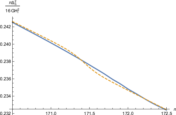
Figure 7: These graphs show the tensor power spectrum for the model of
Figure 5. The left hand figure compares the exact result
(solid blue) with the local slow roll approximation (yellow dashed). The solid blue line on
the right hand graph shows the logarithm of the ratio of to
its local slow roll approximation. The yellow dashed line gives the nonlocal
corrections of expression (63).
Figure 7 shows the tensor power spectrum for the model of
Figure 5. The left hand graph compares the exact result
with the local slow roll approximation. The prominent features of the scalar
power spectrum which can be seen in Figure 6 are several
hundred times smaller, inverted and phase shifted, but they can just be made
out. The right hand graph compares our approximation (63)
for with the exact result. The agreement is again almost
perfect, with the small deviations actually attributable to numerical
roughness in the interpolation of the exact computation, rather than to any
problem with our approximation (63). Correlating tensor
features with their much stronger scalar counterparts might be possible in
the far future and would represent an impressive confirmation of single-scalar
inflation [21].
5 Reconstructing the Geometry
We have so far considered the problem of using the inflationary geometry to
predict the power spectra. Here we wish to consider the inverse problem of
using and to reconstruct
and . (The scalar and its potential can be derived from
and by the formulae given in footnote 1.) It is well to begin by
setting down a few general principles:
1.
Although is measured to 3-digit accuracy,
the tensor power spectrum has yet to be resolved. When is
finally detected it will take a number of years before much precision is
attained. Therefore, reconstruction should be based on ,
with used only to fix the integration constant which gives
the scale of inflation.
2.
The first slow roll parameter is so small that there is no point in
using the exact expression (4) for .
Figure 2 shows that we can ignore the local slow roll correction
factor . Although the nonlocal correction exponent
must be included, Figure 6 shows that
the approximation (64) almost perfect.
3.
The fact that is small and smooth, with small transients,
motivates a hierarchy between , and based
on calculus,
(68)
Hence is insensitive to small errors in , and
is insensitive to small errors in .
Figure 8: Numerical values of exponents 1, 2 and 4 for the model of
Figure 5. The left hand graph gives separate results for
expression (71) in dashed blue, expression (72) in dot-dashed
yellow, and expression (74) in solid green. The right hand graph
shows the sum of all three exponents.
We begin by converting from wave number to , the number of e-foldings
since the beginning of inflation that experienced first horizon crossing.
It is also desirable to factor out the scale of inflation ,
(69)
( is the single number which would come from the tensor power spectrum.)
Based on the three principles we base reconstruction on the formula,
(70)
where the five exponents follow from our approximation (64)
for ,
(71)
(72)
(73)
(74)
(75)
Figure 9: Numerical values of and for
the model of Figure 5. The left hand graph gives
separate results for expression (73) in dashed blue, and expression
(75) in solid yellow. Note that is responsible for
correcting the small, systematic under-prediction of the slow roll
approximation before and after the feature. The right hand graph shows the
sum.
To just reconstruct the Hubble parameter there is no need to include the
correction exponents (71-75). Using only the leading slow
roll terms gives,
(76)
Even for the power spectrum of Figure 6 the reconstruction
of given by expression (76) is barely distinguishable
from the left hand graph of figure 5.
Figure 10: Various choices for the left hand side of the first pass
reconstruction equation for the model of Figure 5. The
left hand graph shows the first pass source
in solid blue with overlaid in dashed yellow. The poor
agreement between the two curves is why using just as
the left hand side of the first pass reconstruction fails to converge when
features are present. The right hand graph shows the much better agreement
between the same source (solid blue) and (dashed yellow).
Not all the exponents (71-75) are equally important.
Figures 8 and 9 show that the set of ,
and are about ten times larger than
and for the model of Figure 5.
That reconstructing features indeed requires the three large exponents is
apparent from Figure 10. Taking the logarithm of (70) and
moving the three large exponents to the left gives,
(77)
This becomes a linear, nonlocal equation for if we drop
and and use expression (76)
for the Hubble parameter,
(78)
The linearity of equation (78) means that it can be solved by
a Green’s function, in spite of being nonlocal. The required Green’s function
becomes a symmetric function of its arguments if we note from Figure 3
and expression (50) that is essentially zero more than
about e-foldings before horizon crossing. The Green’s function
equation is,
(79)
We can solve (78) by integrating against the source on the right
hand side,
(80)
This might be regarded as the first pass of an iterative solution to
(77). After the first pass solution of (78) one would
use the resulting to construct and to evaluate
and on the right hand side of (77).
Then the same Green’s function solution (80) could be used with this
more accurate source to find a more accurate , which would lead
to a more accurate source, and so on.
Figure 11: These graphs show numerical reconstructions of for
the power spectrum of Figure 6. The solid blue line of the left
hand graph shows the exact result while the yellow dashed line gives the result
of integrating — using the first six terms of the sum
over in expression (83) — against the first pass source on the
right hand side of (78). The right hand graph shows the result of
adding the first order improvement — computed using
the first four terms of the sum over in expression (92).
We are not able to solve (79) exactly owing to the factor of
inside the integral. Consideration of Figure 3 suggests
that this troublesome factor might be approximated as a square wave of width
,
(81)
Making the approximation (81) leads to a still-nonlocal equation,
(82)
The “retarded” solution to (82) which avoids exponentially growing
terms is,
(83)
Figure 11 shows the result of using just to
reconstruct with the source taken as the right hand side
of (78).
Figure 12: The solid blue line of the left hand graph shows a numerical evaluation
of the integral of expression (86). The 0th order
approximation of expression (87) is overlaid in large
dots. The solid blue line of the right hand graph shows the deviation . Our fit
of expression (88) is overlaid in large dots.
Further improvement requires a better approximation for the Green’s function
. It is instructive to take the Laplace transform, restoring
the second argument of the Green’s function,
(84)
The Laplace transform of the Green’s function equation (79) is,
(85)
where we define,
(86)
The problem of approximating is therefore related to the
one of approximating (86), and of recognizing the resulting inverse
Laplace transform of . Making the approximation
(81) in (86) gives,
(87)
Figure 12 reveals that this is indeed a good approximation.
Figure 12 also shows that the small residual is well fit by the
function,
(88)
To obtain the first correction to we begin by expanding
in powers of ,
(89)
(90)
(91)
We can recognize the inverse Laplace transform by expanding ,
(92)
Figure 11 shows the effect of using to solve equation (78) approximately for
.
Figure 11 shows that additional improvements are needed before our
technique gives good results for when features
are present. However, our results for are already reasonable,
and those for are staggeringly accurate. For the model of
Figure 5 the largest percentage error on in reconstructing
is , and the percentage error for never exceeds
. This seems considerably better than the General Slow Roll
Approximation [33], or techniques based on local expressions
[34]. A recent proposal based on inverse-scattering
[35] reports percentage errors of of as much as
for flat potentials, and up to when features are present.
It is significant that our Green’s function depends
only on the difference of its arguments, and we just need it over a range
of about ten e-foldings. Further, its Laplace transform is defined by
relations (85-86). Figure 12 shows that
there is only a single, simple pole on the real axis, somewhat below
. If nothing else worked we could therefore evaluate numerically for some and then numerically
compute the inverse Laplace transform,
(93)
No matter how time-consuming the computation proved, it would only need to be
done once.
6 Epilogue
As its title suggests, this paper gives final expression to our formalism
for finding the tree order power spectra by evolving the norm-squared mode
functions [20]. Considered purely as a numerical technique
this is more efficient than evolving the mode functions because it avoids
keeping track of the rapidly fluctuating phase, and because it converges about
twice as fast. Nor is anything lost because the phase can be recovered through
expressions (10) and (20). Our formalism applies not only
to single-scalar inflation but also to any conformally related model, such as
inflation [22], whose power spectra are numerically
identical.
Section 2 reviews our formalism, and explains how to factor out arbitrary
approximate solutions (12) and (22). Section 3 then specializes
to what we believe are the best choices (30-31) for these
approximate solutions. Our results (3-4) for the power
spectra are exact at this stage, with the nonlocal correction exponents
and given by (35).
Section 5 makes the approximation that is small, and that
nonlinear effects can be dropped in the equations (12) and (22)
for the residuals. This results in wonderfully simple, analytic approximations
(63-64) for how the nonlocal correction
exponents depend upon . Figures 6 and
7 exhibit the accuracy of these formulae, even for the model of
Figure 5 which has prominent features. Figure 6
also demonstrates that the local slow roll approximation —
— breaks down badly when features are present, and that it
systematically underestimates even for models
without features. The unmistakable conclusions are:
1.
That quantitative accuracy requires the nonlocal correction exponents
and ; and
2.
That our approximations (63-64) are
valid for any model which is consistent with the bounds on and on the
limits of possible features.
Section 5 explains how our approximation (64) can be used
to reconstruct the geometry from the power spectra. (The scalar and its
potential can be recovered from the formulae of footnote 1.) Further improvements
are needed for accurate reconstructions for derivatives of the first slow roll
parameter, but the undifferentiated parameter is accurate to and our
errors for the Hubble parameter never exceed . This seems much better
than other techniques [33, 34, 35].
Our formalism has many applications because it gives explicit, analytic and
accurate approximations for how the power spectra depend functionally on the
geometry of inflation. For example, our expressions (3-4)
imply an exact relation for the tensor-to-scalar ratio,
(94)
with no local, slow roll corrections. It should be an excellent approximation
to drop and employ the analytic approximation
(64) for .
We have already mentioned the necessity of including the nonlocal correction
exponent to correctly describe features. Our analytic
approximation (64) facilitates precision studies, limited
by the accuracy of the data rather than by the cumbersome connection to
theory. For example, the model of Figure 5 was proposed [28, 29] to account for the deficit in the scalar
power spectrum at , and the excess at ,
which are visible in the data reported from both WMAP [27, 30] and PLANCK [31, 32]. From
Figure 6 we see that the resulting power spectrum indeed
has a deficit at , followed by an excess at .
However, there are weaker features at and .
Do the data show any evidence for these weaker features? If not, to what degree
does their absence rule out the model of Figure 5? And what
sort of model do the data actually support?
A particularly exciting application of our formalism is to exploit the
control it gives over how the mode functions depend upon to
design a new statistic to cross-correlate features in the power spectrum
with non-Gaussianity. This has already been proposed in the context of models
with variable speed of sound [36, 37] but it can
now be done with precision for simple scalar potential models. Of course the
idea is that non-Gaussianity measures self-interaction, which is what a step
in the potential provides. There may be an observable effect which is not
resolvable by generic statistics but could be detected by a precision search.
Another application concerns the far future, after the tensor power spectrum
has been well resolved. Our analytic approximations
(63-64) quantify how the same derivatives of
the first slow roll parameter lead to deviations from the local slow roll
predictions for the tensor and scalar power spectra. Figure 6
shows that these deviations are strongly present in
for models with features. The associated tensor features are much weaker, but
they can just be made out in Figure 7. Demonstrating this
correlation in the data would represent an impressive check on single-scalar
inflation.
In the even farther future it may be possible to resolve one loop corrections
[23]. Comparing these with theory obviously requires a precision
determination of the tree order effect, which is of course possible once the model
of inflation has been fixed. However, one also needs to be able to extract the
potentially large factors of from the propagator, and our
formalism is ideal for that.
Acknowledgements
This work was partially supported by the European Union’s Seventh
Framework Programme (FP7-REGPOT-2012-2013-1) under grant agreement
number 316165; by the European Union’s Horizon 2020 Programme
under grant agreement 669288-SM-GRAV-ERC-2014-ADG;
by NSF grant PHY-1506513; and by the UF’s Institute for
Fundamental Theory.
References
[1]
A. A. Starobinsky,
JETP Lett. 30, 682 (1979)
[Pisma Zh. Eksp. Teor. Fiz. 30, 719 (1979)].
[2]
V. F. Mukhanov and G. V. Chibisov,
JETP Lett. 33, 532 (1981)
[Pisma Zh. Eksp. Teor. Fiz. 33, 549 (1981)].
[3]
R. P. Woodard,
Rept. Prog. Phys. 72, 126002 (2009)
doi:10.1088/0034-4885/72/12/126002
[arXiv:0907.4238 [gr-qc]].
[4]
A. Ashoorioon, P. S. Bhupal Dev and A. Mazumdar,
Mod. Phys. Lett. A 29, no. 30, 1450163 (2014)
doi:10.1142/S0217732314501636
[arXiv:1211.4678 [hep-th]].
[5]
L. M. Krauss and F. Wilczek,
Phys. Rev. D 89, no. 4, 047501 (2014)
doi:10.1103/PhysRevD.89.047501
[arXiv:1309.5343 [hep-th]].
[6]
D. Polarski and A. A. Starobinsky,
Phys. Lett. B 356, 196 (1995)
doi:10.1016/0370-2693(95)00842-9
[astro-ph/9505125].
[7]
J. Garcia-Bellido and D. Wands,
Phys. Rev. D 52, 6739 (1995)
doi:10.1103/PhysRevD.52.6739
[gr-qc/9506050].
[8]
M. Sasaki and E. D. Stewart,
Prog. Theor. Phys. 95, 71 (1996)
doi:10.1143/PTP.95.71
[astro-ph/9507001].
[9]
V. F. Mukhanov, H. A. Feldman and R. H. Brandenberger,
Phys. Rept. 215, 203 (1992).
doi:10.1016/0370-1573(92)90044-Z
[10]
A. R. Liddle and D. H. Lyth,
Phys. Rept. 231, 1 (1993)
doi:10.1016/0370-1573(93)90114-S
[astro-ph/9303019].
[11]
J. E. Lidsey, A. R. Liddle, E. W. Kolb, E. J. Copeland, T. Barreiro and M. Abney,
Rev. Mod. Phys. 69, 373 (1997)
doi:10.1103/RevModPhys.69.373
[astro-ph/9508078].
[12]
A. R. Liddle, P. Parsons and J. D. Barrow,
Phys. Rev. D 50, 7222 (1994)
doi:10.1103/PhysRevD.50.7222
[astro-ph/9408015].
[13]
N. C. Tsamis and R. P. Woodard,
Annals Phys. 267, 145 (1998)
doi:10.1006/aphy.1998.5816
[hep-ph/9712331].
[14]
T. D. Saini, S. Raychaudhury, V. Sahni and A. A. Starobinsky,
Phys. Rev. Lett. 85, 1162 (2000)
doi:10.1103/PhysRevLett.85.1162
[astro-ph/9910231].
[15]
S. Nojiri and S. D. Odintsov,
Gen. Rel. Grav. 38, 1285 (2006)
doi:10.1007/s10714-006-0301-6
[hep-th/0506212].
[16]
R. P. Woodard,
Lect. Notes Phys. 720, 403 (2007)
doi:10.1007/978-3-540-71013-4_14
[astro-ph/0601672].
[17]
Z. K. Guo, N. Ohta and Y. Z. Zhang,
Mod. Phys. Lett. A 22, 883 (2007)
doi:10.1142/S0217732307022839
[astro-ph/0603109].
[18]
D. J. Brooker, N. C. Tsamis and R. P. Woodard,
Phys. Rev. D 93, no. 4, 043503 (2016)
doi:10.1103/PhysRevD.93.043503
[arXiv:1507.07452 [astro-ph.CO]].
[19]
D. J. Brooker, N. C. Tsamis and R. P. Woodard,
arXiv:1605.02729 [gr-qc].
[20]
M. G. Romania, N. C. Tsamis and R. P. Woodard,
JCAP 1208, 029 (2012)
doi:10.1088/1475-7516/2012/08/029
[arXiv:1207.3227 [astro-ph.CO]].
[21]
D. J. Brooker, N. C. Tsamis and R. P. Woodard,
arXiv:1603.06399 [astro-ph.CO].
[22]
D. J. Brooker, S. D. Odintsov and R. P. Woodard,
Nucl. Phys. B 911, 318 (2016)
doi:10.1016/j.nuclphysb.2016.08.010
[arXiv:1606.05879 [gr-qc]].
[23]
R. P. Woodard,
Int. J. Mod. Phys. D 23, no. 09, 1430020 (2014)
doi:10.1142/S0218271814300201
[arXiv:1407.4748 [gr-qc]].
[24]
P. A. R. Ade et al. [BICEP2 and Planck Collaborations],
Phys. Rev. Lett. 114, 101301 (2015)
doi:10.1103/PhysRevLett.114.101301
[arXiv:1502.00612 [astro-ph.CO]].
[25]
P. A. R. Ade et al. [Planck Collaboration],
Astron. Astrophys. 594, A13 (2016)
doi:10.1051/0004-6361/201525830
[arXiv:1502.01589 [astro-ph.CO]].
[26]
P. A. R. Ade et al. [Planck Collaboration],
arXiv:1502.02114 [astro-ph.CO].
[27]
L. Covi, J. Hamann, A. Melchiorri, A. Slosar and I. Sorbera,
Phys. Rev. D 74, 083509 (2006)
doi:10.1103/PhysRevD.74.083509
[astro-ph/0606452].
[28]
J. A. Adams, B. Cresswell and R. Easther,
Phys. Rev. D 64, 123514 (2001)
doi:10.1103/PhysRevD.64.123514
[astro-ph/0102236].
[29]
M. J. Mortonson, C. Dvorkin, H. V. Peiris and W. Hu,
Phys. Rev. D 79, 103519 (2009)
doi:10.1103/PhysRevD.79.103519
[arXiv:0903.4920 [astro-ph.CO]].
[30]
J. Hamann, L. Covi, A. Melchiorri and A. Slosar,
Phys. Rev. D 76, 023503 (2007)
doi:10.1103/PhysRevD.76.023503
[astro-ph/0701380].
[31]
D. K. Hazra, A. Shafieloo, G. F. Smoot and A. A. Starobinsky,
JCAP 1408, 048 (2014)
doi:10.1088/1475-7516/2014/08/048
[arXiv:1405.2012 [astro-ph.CO]].
[32]
D. K. Hazra, A. Shafieloo, G. F. Smoot and A. A. Starobinsky,
JCAP 1609, no. 09, 009 (2016)
doi:10.1088/1475-7516/2016/09/009
[arXiv:1605.02106 [astro-ph.CO]].
[33]
K. Kadota, S. Dodelson, W. Hu and E. D. Stewart,
Phys. Rev. D 72, 023510 (2005)
doi:10.1103/PhysRevD.72.023510
[astro-ph/0505158].
[34]
J. D. Barrow and A. Paliathanasis,
arXiv:1611.06680 [gr-qc].
[35]
J. Mastache, F. Zago and A. Kosowsky,
Phys. Rev. D 95, no. 6, 063511 (2017)
doi:10.1103/PhysRevD.95.063511
[arXiv:1611.03957 [astro-ph.CO]].
[36]
A. Achúcarro, J. O. Gong, G. A. Palma and S. P. Patil,
Phys. Rev. D 87, no. 12, 121301 (2013)
doi:10.1103/PhysRevD.87.121301
[arXiv:1211.5619 [astro-ph.CO]].
[37]
J. Torrado, B. Hu and A. Achucarro,
arXiv:1611.10350 [astro-ph.CO].