Stability Analysis of Constrained Optimization Dynamics via Passivity Techniques
Abstract
In this paper, we present passivity based convergence analysis of continuous time primal-dual gradient method for convex optimization problems. We first show that a convex optimization problem with only affine equality constraints admit a Brayton Moser formulation. This observation leads to a new passivity property derived from a Krasovskii type storage function. Secondly, the inequality constraints are modeled as a state dependent switching system. Using hybrid methods, it is shown that each switching mode is passive and the passivity of the system is preserved under arbitrary switching. Finally, the two systems, (i) one derived from the Brayton Moser formulation and (ii) the state dependent switching system, are interconnected in a power conserving way. The resulting trajectories of the overall system are shown to converge asymptotically, to the optimal solution of the convex optimization problem. The proposed methodology is applied to an energy management problem in buildings and simulations are provided for corroboration.
1 Introduction
The applications of convex optimization are ubiquitous in various fields of research [1] such as, resource allocation [2], utility maximization [3] etc. Numerous methods are proposed to solve these optimization problems [4]. Solution techniques in a distributed setting have gained importance in recent times[5]. One of the standard tools for designing algorithms to solve such optimization problems is through primal-dual gradient method [6, 7]. Gradient based methods are a well known class of mathematical routines for solving convex optimization problems. From a control and dynamics perspective, these primal dual algorithms have much to offer in terms of using tools from system theory to have better understanding of the underlying dynamics. Passivity, a system theoretic tool has been widely used for studying dynamical systems as it relates to energy conservation and used for attaining classical control objectives such as stabilization and performance.
The convergence of gradient based methods and Lyapunov stability relate the solution of the optimization problem to the equilibrium point of a dynamical system. The Krasovskii-Lyapunov function is particularly suited for establishing stability of the continuous time gradient laws, as the equilibrium point (or solution of the optimization problem) is not known apriori. In [8], the authors used this Krasovskii Lyapunov function and hybrid Lasalle’s invariance principle [9] to prove asymptotic stability of a network optimization problem. The gradient structure of the primal-dual equations characterizing the optima of a convex optimization with only equality constraint admit a Brayton Moser (BM) form. Further, using the duality between energy and co-energy the BM form is partially transformed into a port-Hamiltonian (pH) form [10, 11]. These transformations pave the way for passivity/stability analysis using (i) the invariance principle for discontinuous Caratheodory systems [12] and (ii) an incremental passivity property for the misfit dynamics. In [13], the authors provided robustness analysis for primal-dual dynamics of convex optimization problem with only equality constraint. A brief list of applications of primal dual gradient methods is given below: in the context of power systems, these methods have been used to achieve optimal load sharing [14], investigating effects of real-time pricing on stability and volatility of electricity markets [15], and stability analysis of integrated power markets with physical dynamics[11]. In [16], primal-dual gradient method is used to solve the energy management problem in application to HVAC systems.
Increasing energy demand, with supply constraints brings consumers and producers to behave in a manner of maximizing social welfare. In the context of building energy management system, the buildings (consumers) try to optimize their set-point to maximize comfort, whereas utilities try to reduce their generation costs. Traditionally, conventional generators were employed to meet the additional demand. With increasing demand side management programs, utilities provide incentives to consumers to lower the overall power demand. This results in reducing load during the time when prices are high. These programs lead to a process which involve both the supply and the demand-side resources to minimize the overall cost. Building systems being one of the strong contenders for providing ancillary services to the grid [17] in which heating ventilating and airconditioning (HVAC) systems play a significant role, as they account for approximately 30-40% of the total energy demand. There is a vast amount of literature on demand response (DR) strategies in maintaining optimal balance between supply and demand at all times. An overview on the types of DR and taxonomy for demand side management is described in [18]. Real-time pricing based demand response (DR) application [19] has been deployed in smart meters of residential homes to have direct control of loads such as air conditioners etc. Recently the authors [20] have proposed the Brayton - Moser (BM) formulation for modeling and stability analysis of HVAC subsystems.
Motivations and Main contributions
In any stabilization problem, whether it is to stabilize a system to an equilibrium point or to an operating point, the velocities must converge asymptotically to zero. This observation motivates the need for storage functions defined explicitly in velocities. A good candidate, in general, is a positive definite quadratic function of velocities. In [21], the authors showed that for systems specified in BM form a new passivity property can be derived, with differentiation at both the port variables. In this paper, we employ a similar methodology to derive passive maps directly from the BM form of a convex optimization problem with only equality constraints. The primal-dual dynamics of the inequality constraint is modelled as a state dependent switching system. We first show that each switching mode is passive and the passivity of the system is preserved under arbitrary switching using hybrid passivity tools, a methodology similar to switched Lyapunov functions for stability analysis of switch system. Finally, the two systems, (i) one derived from the Brayton Moser formulation and (ii) the state dependent switching system, are interconnected in a manner such that the equilibrium is the solution of the convex optimization problem.
As a case study, we apply primal-dual methodology to a social welfare problem associated with building energy management system. From an application stand point, BM framework presents a design methodology for stabilization [20] of HVAC subsystems. This motivates us to analyze the social-welfare problem, in the context of building systems, formulated as a trade-off between user comfort and generation costs.
An elaborate version of this manuscript can be found at [22].
2 Preliminaries
Brayton-Moser formulation
Consider the standard representation of a dynamical system in Brayton-Moser (BM) formulation
| (1) |
the system state vector and the input vector (). is a scalar function of the state, which has the units of power, also referred to as mixed potential function [10]. and . In BM formulation we represent the system dynamics in pseudo-gradient form, ( and are indefinite). Therefore can not be used as a Lyapunov function for stability analysis. A way of constructing a suitable Lyapunov function involves finding and [23, 21] such that
| (2) |
3 Passivity based formulation of the optimization problem
Consider the following constrained optimization problem
| (3) | ||||||
where is continuously differentiable and strictly convex and is affine. Assume
- (i)
that the objective function has a positive definite Hessian
- (ii)
The solution is an optimal solution to (3) if there exists such that the following Karush-Kuhn-Tucker (KKT) conditions are satisfied.
| (4) |
The Lagrangian of (3) is given by
| (5) |
Since strong duality holds for (3), is a saddle point of the Lagrangian if and only if is an optimal solution to (3) and is optimal solution to its dual problem. Consider the following dynamics
| (6) |
where are positive definite matrices and input . The unforced system () of equations (6) represent primal-dual dynamics corresponding to (5) and the equilibrium corresponds to the KKT conditions (4).
3.1 The Brayton Moser formulation:
Denote . The continuous time gradient laws (6), associated with (3), naturally admit a Brayton-Moser (BM) formulation
| (7) |
with and is a scalar function of the state, which has the units of power, also referred to as mixed potential function [10].
Proposition 3.1.
The proof of this and other propositions are given in Appendix at the end of this paper.
3.2 Inequality constraints
We now define the inequality constraint as the following hybrid dynamics
| (8) |
where and . The positive projection of can be written as
Note that the discontinuity in the above equations occurs when and , the value of switches from to . To make this more visible, we redefine these equations equivalently as follows;
| (9) |
The projection is said to be active in the second case. Let represent the power set of , then we define the function as follows
| (10) |
where the projection is active. With representing the switching signal, equation (8) now takes the form of a switched system
| (11) |
The overall dynamics of the inequality constraints can be written in a compact form as:
| (12) |
where and are components of and respectively. A strictly passive system can be proven to be asymptotically stable, with Lyapunov function as the storage function. But in the case of switching systems its misleading. It is well known that a sufficient condition for a switched system to be passive system is that the storage function should be common for all the individual subsystems [24]. In general it is not easy to find such storage functions. Here we use passivity property defined with ‘multiple storage functions’[25]. Consider the following storage function(s)
| (13) |
Proposition 3.2.
The switched system (12) is passive with multiple storage functions (defined one for each switching state ), input port and output port where . That is, for each with the property that for every pair of switching times , such that and for , we have
| (14) |
Proposition 3.3.
3.3 The overall optimization problem:
The most interesting property of passive systems is their modular nature. One can define power conserving interconnections (such as Newton law’s or Kirchoff’s current/voltage laws) between these systems, and show that the overall system is passive and there by stability. In this subsection we define a power conserving interconnection between passive systems associated with optimization problem with an equality constraint (6) and an inequality constraint (8).
Proposition 3.4.
Consider the interconnection of passive systems (6) and (8), via the following interconnection constraints . The interconnected system is then passive with port variables , . Moreover for the interconnected system represents the primal-dual gradient dynamics of the optimization problem
| (15) | ||||||
and the trajectories converge asymptotically to the optimal solution of (15).
4 Building Energy Management Formulation
This section describes the mathematical formulation of the energy management problem of building HVAC systems. The problem is formulated by taking into account the interaction between the multiple consumers and a single producer in achieving social welfare. The rising opportunities for demand side flexibility enables the consumers to manage their load to reduce their costs, in this context, we model the coalition by group of consumers in order to have access to wholesale energy markets. The coalition coordinator or energy provider purchases the electricity from wholesale energy markets and resells to each member of the coalition using a simple price structure. In this paper we consider a time-of-use (TOU) pricing. A schematic representation of the interaction between coalition coordinator and group of consumers is shown in Fig. 1. Furthermore, each member of the coalition tries to maximize his own benefit by contributing to overall demand reduction. In order to illustrate the energy management problem, we consider a simulated medium sized commercial building with different zones. The zone thermal dynamics is one of the essential component of the modeling building energy systems.

4.1 Thermal dynamics of building
The thermal dynamics of a multi-zone building can be represented using a resistance-capacitance network and the governing dynamics are given by [20]:
| (16) |
where denotes all resistors connected to the capacitor (includes zone and surface capacitances), is the temperature of the zone and, denotes the ambient temperature. is the thermal capacitance of the zone, is the thermal resistance between zone and zone , is the thermal resistance between zone and ambient conditions, is the heating/cooling input to the zone and denotes the heat gain due to sources such as solar, occupancy etc.
4.2 Problem formulation
The optimization problem: The energy management problem is formulated as a group of consumers that form a coalition and a energy provider or coalition coordinator who purchases electricity from the wholesale markets through contracts. The objective is to define the total welfare function of the coalition of consumers under the operational and market clearing constraints. The optimization problems for each consumer and producer at each time slot is given as below. The optimization problem for each consumer is given as follows
Each of these consumers has a private utility function , which represents the utility the consumer derives by consumption of units of power. stands for the market price, is strictly concave function. The objective of energy provider is to maximize his profits and is given by
where, denotes the total supply available to the consumers, N denotes the number of consumers, is strictly convex function . Once we have the consumer and producer cost functions, the social welfare problem is formulated as the net benefits of the consumers and producer [26], and is given by
Using the generic formulation discussed above, the energy management of HVAC system is formulated by considering the discomfort and generation costs as consumer and producer utility functions, respectively [16]. This can be formulated as
| (17) | ||||||
where, , () and denotes the conversion factor from energy consumption to energy demand [27]. The coefficients determines the tradeoff between cost and comfort [28]. The steady state dynamics of (16) is considered to relate energy supply and demand. In the compact notation, the Lagrangian is given as
| (18) | |||||
where, . As discussed in Section 3.3, the primal dual dynamics of (18) is given as
| (19) | |||||
Proposition 4.1.
5 Simulation results
In this section, a simulated study is conducted using a building model emulating the ERS test-bed [29], which represents a small-sized commercial building as shown in Fig. 2.

This simulated model consists of two side-by-side independent and similar zones marked as A and B and distributed in four directions, East, South, West, and North, respectively. These zones are served using two air handling units (AHU) marked A and B, where each AHU will be serving four Variable Air Volume systems (AHU A serving 4 zones (A) in different directions). For simulation purpose, we consider four zones marked as A, distributed in four different directions supplied by a single air handling unit (AHU (A)). The parameters used for the simulation is shown in Table 1.
| , , , | 30, 18, 24, 20.5 |
|---|---|
| Inertial time constants (, , ,,) | 1 |
| , , | 0.5, 0, 0 |
| , , , | 40, 0.5, 11.5, 3 |
To illustrate the effect of load reduction during a price surge, we consider a simulated TOU pricing. TOU pricing essentially provides consumers with different rates at different times in a 24 hour period. Fig. 4 shows the convergence of the algorithm to its optimal value and also the interplay between supply and demand.
Remark 1.
In this study we have four zones, each zone temperature has an upper and lower bound, giving rise to eight inequality constraints. In Figure 3 we have plotted the time evolution of their corresponding Lagrange variables , . Let } denote the ordered sequence of time instances where the Lagrange variables ’s converge to zero.
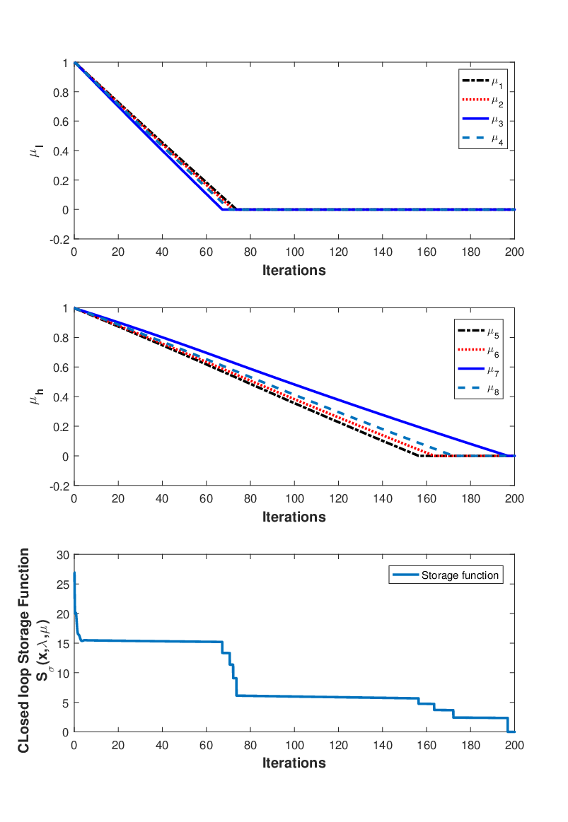
The resulting change in the active sets (switching modes) is captured by the switching signal . In the current scenario, the switching signal have eight different switching modes, and a storage function is defined for each one (refer to Table 2). Figure 3 shows that the closed loop storage function decreases, discontinuously. This discontinuity appears because, at the end of each switching mode, we are switching to a new storage function that is strictly less than the current one. This is coherent with the Proposition 3.2, where passivity property is defined with ‘multiple storage functions’.
| 0 |

In order to evaluate the proposed algorithm for the 24 hour period, we consider the internal load profile as shown in Fig. 5 which is the sum of heat gains due to occupancy and solar radiation. The occupancy load is computed based on the simulated test bed requirements based on [29] using the fraction of total occupancy profile. Similarly the solar load is calculated based on the global horizontal irradiance data collected from [30]. The outside air temperature profile [30] for summer is considered as shown in Fig. 6. The temperature profile for a particular zone (East A) is shown in Fig. 6 to illustrate the zone behavior to the TOU pricing for a hot summer day. It can be seen that during the time when prices are high the zone temperatures vary while contributing to the overall demand reduction.
As a result there is a reduction in cooling load of the building as shown in Fig. 7 in comparison to the building when there is no energy management. Hence, the proposed algorithm effectively reduces the peak load, resulting in overall cost reduction.
6 Conclusions
Starting from an optimization problem with equality constraint we have shown that their primal-dual equations have a naturally existing Brayton Moser representation. Using the interconnection properties of BM systems we extended the optimization problem to include inequality constraints. The overall convergence is guaranteed by proving the asymptotic stability of individual subsystems, whose Lyapunov functions derived from BM formulation have their roots in Krasovskii method. This approach is supported by energy management problem in buildings to reduce the overall demand by varying the zone temperature values during the high prices. This approach further lends itself to include the distributed energy resources such as photo-voltaic systems, etc., as well as battery energy storage into the buildings to find the optimal decisions to benefit both consumers and producers.
APPENDIX
A. Proof of Proposition 3.1:
In BM formulation we represent the system dynamics in pseudo-gradient form, ( and are indefinite). Therefore can not be used as a Lyapunov function for stability analysis. A way of constructing a suitable Lyapunov function involves finding and [23, 21] such that
| (20) |
Considering (20) with and we have
| (21) |
The time derivative of the storage function (21) along the system of equations (6) can be computed as
which implies that the system (6) is passive. Further for we have ( is some constant). Using this in the first equation of (6) we get that is a constant, proving asymptotic stability of .
B. Proof of Proposition 3.2
We start with analyzing the passivity property for a time interval say with fixed . The time derivative of the storage function is
In step two we use (which is true since , if ) and in step three we use the convexity of and non-negativity of the . The above inequality can be equivalently written as
| (22) |
Hence, the system of equation (12) represent a finite family of passive systems and (13) represents their corresponding storage functions.
Since this is not sufficient to prove the passivity property of (12), we further need to analyse the behaviour of the storage functions at all switching times. Let denotes current active projection set as defined in (10), then we have the following scenarios:
- (i)
For some , let the projection of constraint () becomes active (i.e reaches when ) at time . This implies a new element is added to the projection set, . The term in the storage function corresponding to this will not appear in (13) as . This happens discontinuously because switches from to . Hence
(23) - (ii)
In the case when the projection of an active constraint becomes inactive i.e , a new term is added to the summation of the storage function (13). But this happens in a continuous way because has to increase from to by crossing . By continuity argument we have
(24)

Now consider a as given in the proposition. Now consider a with the property that for every pair of switching times , such that and for . We assume that there are switching times between and . Noting that the storage function is not increasing at switching times we have,
Above we used (22), (23) and (24). We thus conclude the system is passive with port variables .
C. Proof of Proposition 3.3
From (6), (23) and (24) in Proposition 3.2, we can infer that the Lyapunov function (13) is non-increasing for a constant , concluding Lyapunov stability. Now we use hybrid Lasalle’s theorem condition [9] to show that is the maximal positively invariant set, defined by
- (i)
for fixed . This is can be verified by substituting a constant in (6).
- (ii)
Consider the quadratic norm . Next, using (8), (9) and (17) together with , we show that the is non-increasing
This implies that the trajectories of (8) are bounded for . If , increases linearly, contradicting the boundedness of the trajectories. The proof follows by noting that conditions in (25) represent set.
D. Proof of Proposition 3.4
Define the storage function . The time differential of is
The interconnection of (6) and (8), with , gives
| (26) |
which represent the primal-dual gradient dynamics of (3).
Hence the overall system take the form of primal-dual gradient dynamics representing optimization problem with both equality and in-equality constraint (15).
When , for the interconnected system. Stability can thus be concluded using the relation between passivity and stability [31] and Propositions 3.2, 3.3.
References
- [1] A. Ben-Tal and A. Nemirovski, Lectures on modern convex optimization: analysis, algorithms, and engineering applications. SIAM, 2001.
- [2] T. Ibaraki and N. Katoh, Resource allocation problems: algorithmic approaches. MIT press, 1988.
- [3] F. P. Kelly, A. K. Maulloo, and D. K. Tan, “Rate control for communication networks: shadow prices, proportional fairness and stability,” Journal of the Operational Research society, vol. 49, no. 3, pp. 237–252, 1998.
- [4] S. Boyd and L. Vandenberghe, Convex optimization. Cambridge university press, 2004.
- [5] L. Xiao and S. Boyd, “Optimal scaling of a gradient method for distributed resource allocation,” Journal of optimization theory and applications, vol. 129, no. 3, pp. 469–488, 2006.
- [6] T. Kose, “Solutions of saddle value problems by differential equations,” Econometrica, Journal of the Econometric Society, pp. 59–70, 1956.
- [7] K. J. Arrow, L. Hurwicz, H. Uzawa, and H. B. Chenery, “Studies in linear and non-linear programming,” 1958.
- [8] D. Feijer and F. Paganini, “Stability of primal–dual gradient dynamics and applications to network optimization,” Automatica, vol. 46, no. 12, pp. 1974–1981, 2010.
- [9] J. Lygeros, K. H. Johansson, S. N. Simic, J. Zhang, and S. S. Sastry, “Dynamical properties of hybrid automata,” IEEE Transactions on automatic control, vol. 48, no. 1, pp. 2–17, 2003.
- [10] D. Jeltsema and J. M. Scherpen, “Multidomain modeling of nonlinear networks and systems,” IEEE Control Systems Magazine, vol. 29, no. 4, 2009.
- [11] T. Stegink, C. De Persis, and A. van der Schaft, “A unifying energy-based approach to stability of power grids with market dynamics,” IEEE Transactions on Automatic Control, vol. PP, no. 99, pp. 1–11, 2016.
- [12] A. Cherukuri, E. Mallada, and J. Cortés, “Asymptotic convergence of constrained primal–dual dynamics,” Systems & Control Letters, vol. 87, pp. 10–15, 2016.
- [13] J. W. Simpson-Porco, “Input/output analysis of primal-dual gradient algorithms,” in Communication, Control, and Computing (Allerton), 2016 54th Annual Allerton Conference on. IEEE, 2016, pp. 219–224.
- [14] P. Yi, Y. Hong, and F. Liu, “Distributed gradient algorithm for constrained optimization with application to load sharing in power systems,” Systems & Control Letters, vol. 83, pp. 45–52, 2015.
- [15] M. Roozbehani, M. A. Dahleh, and S. K. Mitter, “Volatility of power grids under real-time pricing,” IEEE Transactions on Power Systems, vol. 27, no. 4, pp. 1926–1940, 2012.
- [16] K. Ma, G. Hu, and C. J. Spanos, “Energy management considering load operations and forecast errors with application to hvac systems,” IEEE Transactions on Smart Grid, vol. PP, no. 99, pp. 1–10, 2016.
- [17] H. Hao, A. Kowli, Y. Lin, P. Barooah, and S. Meyn, “Ancillary service for the grid via control of commercial building hvac systems,” in American Control Conference (ACC), 2013. IEEE, 2013, pp. 467–472.
- [18] P. Palensky and D. Dietrich, “Demand side management: Demand response, intelligent energy systems, and smart loads,” IEEE transactions on industrial informatics, vol. 7, no. 3, pp. 381–388, 2011.
- [19] J. L. Mathieu, S. Koch, and D. S. Callaway, “State estimation and control of electric loads to manage real-time energy imbalance,” IEEE Transactions on Power Systems, vol. 28, no. 1, pp. 430–440, 2013.
- [20] V. Chinde, K. Kosaraju, A. Kelkar, R. Pasumarthy, S. Sarkar, and N. Singh, “Building hvac systems control using power shaping approach,” in American Control Conference (ACC), 2016. IEEE, 2016, pp. 599–604.
- [21] K. Kosaraju, R. Pasumarthy, N. Singh, and A. Fradkov, “Control using new passivity property with differentiation at both ports,” Indian Control Conference (ICC), pp. 7–11, 2017.
- [22] K. Kosaraju, V. Chinde, R. Pasumarthy, A. Kelkar, and N. Singh, “Stability analysis of constrained optimizationproblem using passivity approach,” arXiv:1708.03212, 2017.
- [23] R. Ortega, D. Jeltsema, and J. M. Scherpen, “Power shaping: A new paradigm for stabilization of nonlinear rlc circuits,” IEEE Transactions on Automatic Control, vol. 48, no. 10, pp. 1762–1767, 2003.
- [24] J. Zhao and D. J. Hill, “A notion of passivity for switched systems with state-dependent switching,” Journal of control theory and applications, vol. 4, no. 1, pp. 70–75, 2006.
- [25] M. Zefran, F. Bullo, and M. Stein, “A notion of passivity for hybrid systems,” IEEE Conference on Decision and Control (CDC), 2001.
- [26] E. Wei, “Distributed optimization and market analysis of networked systems,” Ph.D. dissertation, Massachusetts Institute of Technology, 2014.
- [27] G. P. Henze and M. Krarti, “Predictive optimal control of active and passive building thermal storage inventory,” Architectural Engineering–Faculty Publications, p. 1, 2003.
- [28] R. P. Hämäläinen, J. Mäntysaari, J. Ruusunen, and P.-O. Pineau, “Cooperative consumers in a deregulated electricity market—dynamic consumption strategies and price coordination,” Energy, vol. 25, no. 9, pp. 857–875, 2000.
- [29] ERS, “Energy Resource Station Technical Description,” http://www.iowaenergycenter.org/energy-resource-station-ers/, 2015.
- [30] S. Wilcox and W. Marion, Users manual for TMY3 data sets. National Renewable Energy Laboratory Golden, CO, 2008.
- [31] A. J. van der Schaft, “L2-gain and passivity techniques in nonlinear control.” Springer, London, 2000.