跳到论文正文
W Papers独立论文阅读器 arXiv:1708.03060 论文正文 计算阅读时间 · 0%
引用这篇论文根据当前论文元数据生成,正式投稿前建议核对。


License: CC BY 4.0
arXiv:1708.03060v2 [math.AG] 24 Apr 2020

Initial degenerations of Grassmannians

Daniel Corey Note: UW-Madison, Van Vleck Hall, 480 Lincoln Dr. Madison, WI 53706. dcorey@math.wisc.edu
Abstract

We construct closed immersions from initial degenerations of Gr0⁡(d,n)\Gr_{0}(d,n)—the open cell in the Grassmannian Gr⁡(d,n)\Gr(d,n) given by the nonvanishing of all Plücker coordinates—to limits of thin Schubert cells associated to diagrams induced by the face poset of the corresponding tropical linear space. These are isomorphisms when (d,n)(d,n) equals (2,n)(2,n), (3,6)(3,6) and (3,7)(3,7). As an application we prove Gr0⁡(3,7)\Gr_{0}(3,7) is schön, and the Chow quotient of Gr⁡(3,7)\Gr(3,7) by the maximal torus in PGL(7)\operatorname*{PGL}(7) is the log canonical compactification of the moduli space of 7 points in ℙ2\mathbb{P}^{2} in linear general position, making progress on a conjecture of Hacking, Keel, and Tevelev.

Keywords: Grassmannians, initial degenerations, thin Schubert cells, matroids, Chow quotient, log canonical compactification.

Mathematics Subject Classification: 14T05 (primary), 14M15, 14E25 (secondary).

1 Introduction

Let Gr⁡(d,n)\Gr(d,n) be the Grassmannian of dd-dimensional subspaces of 𝐤n\mathbf{k}^{n}, for an algebraically closed field 𝐤\mathbf{k}, and Gr0⁡(d,n)\Gr_{0}(d,n) the open cell given by the nonvanishing of all Plücker coordinates. We consider its tropicalization TGr0⁡(d,n)\TGr_{0}(d,n) through two frameworks. Via Gröbner theory, TGr0⁡(d,n)\TGr_{0}(d,n) consists of those w∈∧dℝnw\in\wedge^{d}{\mathbb{R}}^{n} such that the initial degeneration inw⁡Gr0⁡(d,n)\inw_{w}\Gr_{0}(d,n) is nonempty. Alternatively, TGr0⁡(d,n)\TGr_{0}(d,n) has a modular interpretation as the space of dd-dimensional tropical linear subspaces of ℝn{\mathbb{R}}^{n} that are realizable over valued extensions of 𝐤\mathbf{k} [35]. The goal of this paper is to study initial degenerations of Gr0⁡(d,n)\Gr_{0}(d,n) via their relation to tropical linear spaces.

Suppose w∈TGr0⁡(d,n)w\in\TGr_{0}(d,n) and LwL_{w} is the corresponding tropical linear space. Then ww induces a regular subdivision Δw\Delta_{w} of the hypersimplex Δ⁡(d,n)⊂ℝn\Delta(d,n)\subset{\mathbb{R}}^{n} into matroid polytopes, and there is a bijection between the bounded cells of LwL_{w} and the internal cells of Δw\Delta_{w}, reversing the face order [34]. Equipping TGr0⁡(d,n)\TGr_{0}(d,n) with its Gröbner fan structure, inw⁡Gr0⁡(d,n)\inw_{w}\Gr_{0}(d,n) and Δw\Delta_{w} depend only on the cone of TGr0⁡(d,n)\TGr_{0}(d,n) that contains ww in its relative interior [38].

The collection of all subspaces realizing a matroid MM defines a locally closed subscheme GrM⊂Gr⁡(d,n)\Gr_{M}\subset\Gr(d,n) called the thin Schubert cell of MM. Let us describe an inverse system of thin Schubert cells associated to the matroid subdivision Δw\Delta_{w}. Given a matroid polytope Q⊂Δ⁡(d,n)Q\subset\Delta(d,n), write MQM_{Q} for its matroid and ρMQ\rho_{M_{Q}} for the rank function. Any facet of QQ has the form Q′=Q∩{∑i∈ηxi=ρM(η)}Q^{\prime}=Q\cap\{\sum_{i\in\eta}x_{i}=\rho_{M}(\eta)\} for some η⊂[n]:={0,1,…,n−1}\eta\subset[n]:=\{0,1,\ldots,n-1\}, and MQ′M_{Q^{\prime}} decomposes as a direct sum of the contraction MQ/ηM_{Q}/\eta and restriction MQ|ηM_{Q}|\eta [10]. If F∈Gr⁡(d,n)F\in\Gr(d,n) realizes MQM_{Q} and μ=[n]∖η\mu=[n]\setminus\eta, then F∩𝐤μF\cap\mathbf{k}^{\mu} and F/(F∩𝐤μ)F/(F\cap\mathbf{k}^{\mu}) realize MQ/ηM_{Q}/\eta and MQ|ηM_{Q}|\eta, respectively. We have a morphism

GrMQ→GrMQ′F↦(F∩𝐤μ)⊕F/(F∩𝐤μ).\displaystyle\Gr_{M_{Q}}\to\Gr_{M_{Q^{\prime}}}\hskip 30.0ptF\mapsto(F\cap\mathbf{k}^{\mu})\oplus F/(F\cap\mathbf{k}^{\mu}).

Thus {GrMQ|Q∈Δw}\{\Gr_{M_{Q}}\,|\,Q\in\Delta_{w}\} defines an inverse system, and we may form the limit lim←Q∈Δw⁡GrMQ\varprojlim_{Q\in\Delta_{w}}\Gr_{M_{Q}}.

Theorem 1.1.

For w∈TGr0⁡(d,n)w\in\TGr_{0}(d,n), there is a closed immersion

ψw:inw⁡Gr0⁡(d,n)↪lim←Q∈Δw⁡GrMQ.\psi_{w}:\inw_{w}\Gr_{0}(d,n)\hookrightarrow\varprojlim_{Q\in\Delta_{w}}\Gr_{M_{Q}}.

The morphisms GrMQ→GrMQ′\Gr_{M_{Q}}\to\Gr_{M_{Q^{\prime}}} and limit  lim←Q∈Δw⁡GrMQ\varprojlim_{Q\in\Delta_{w}}\Gr_{M_{Q}} originally appear in [25]. This limit parameterizes collections of subspaces {FQ∈GrMQ|Q∈Δw}\{F_{Q}\in\Gr_{M_{Q}}\,|\,Q\in\Delta_{w}\}, such that, if Q1Q_{1} and Q2Q_{2} share a common face defined by ∑i∈ηxi=ρMQ1​(η)=d−ρMQ2​(μ)\sum_{i\in\eta}x_{i}=\rho_{M_{Q_{1}}}(\eta)=d-\rho_{M_{Q_{2}}}(\mu) with μ=[n]∖η\mu=[n]\setminus\eta, then

FQ1/(FQ1∩𝐤μ)=FQ2∩𝐤η and FQ2/(FQ2∩𝐤μ)=FQ1∩𝐤ηF_{Q_{1}}/(F_{Q_{1}}\cap\mathbf{k}^{\mu})=F_{Q_{2}}\cap\mathbf{k}^{\eta}\hskip 15.0pt\text{ and }\hskip 15.0ptF_{Q_{2}}/(F_{Q_{2}}\cap\mathbf{k}^{\mu})=F_{Q_{1}}\cap\mathbf{k}^{\eta}

under the identifications 𝐤n/𝐤μ=𝐤η\mathbf{k}^{n}/\mathbf{k}^{\mu}=\mathbf{k}^{\eta} and 𝐤n/𝐤η=𝐤μ\mathbf{k}^{n}/\mathbf{k}^{\eta}=\mathbf{k}^{\mu}.

In the construction of a morphism to lim←Q∈Δw⁡GrMQ\varprojlim_{Q\in\Delta_{w}}\Gr_{M_{Q}}, it suffices to construct compatible morphisms inw⁡Gr0⁡(d,n)→GrMQ\inw_{w}\Gr_{0}(d,n)\to\Gr_{M_{Q}} whenever QQ is an internal cell of Δw\Delta_{w}. Let us sketch a geometric characterization of these morphisms. Choose a 𝐤\mathbf{k}-point xx of inw⁡Gr0⁡(d,n)\inw_{w}\Gr_{0}(d,n) and set 𝕂=𝐤⁡((tℝ))\mathbb{K}=\mathbf{k}(\!(t^{{\mathbb{R}}})\!). By surjectivity of exploded tropicalization [31], there is a 𝕂\mathbb{K}-point pp of Gr0⁡(d,n)\Gr_{0}(d,n) such that 𝔗​𝔯​𝔬​𝔭​(p)=x\mathfrak{Trop}(p)=x; because 𝕂\mathbb{K} is a generalized power series field, 𝔗​𝔯​𝔬​𝔭​(p)\mathfrak{Trop}(p) is simply the vector of lead coefficients. The Plücker vector pp defines a linear subspace FpF_{p} of (𝕂∗)n(\mathbb{K}^{*})^{n} whose tropicalization is LwL_{w}. For any vv in the bounded cell of LwL_{w} dual to QQ, the closure of inv⁡(Fp)\inw_{v}(F_{p}) in 𝐤n\mathbf{k}^{n} is a linear realization of MQM_{Q}. The morphism inw⁡Gr0⁡(d,n)→GrMQ\inw_{w}\Gr_{0}(d,n)\to\Gr_{M_{Q}} sends xx to inv⁡(Fp)\inw_{v}(F_{p}). We will produce a scheme-theoretic construction of these morphisms in Section 3, and provide compatibility with this geometric description in Remark 3.6.

Our main application of Theorem 1.1 is to determine smoothness and irreducibility of initial degenerations of Grassmannians, especially for Gr0⁡(3,7)\Gr_{0}(3,7). Because TGr0⁡(d,n)\TGr_{0}(d,n) is sensitive to the characteristic of the underlying field, we assume that char⁡𝐤=0\operatorname{char}\mathbf{k}=0.

Theorem 1.2.

The initial degenerations of Gr0⁡(3,7)\Gr_{0}(3,7) are smooth and irreducible.

The computation of TGr0⁡(3,7)\TGr_{0}(3,7) in [17] allows us to compute the initial degenerations of Gr0⁡(3,7)\Gr_{0}(3,7) and matroid subdivisions of Δ⁡(3,7)\Delta(3,7). Given the size of the initial ideals, determining smoothness and irreducibility of the inw⁡Gr0⁡(3,7)\inw_{w}\Gr_{0}(3,7) directly is impractical, even with computer assistance. In comparison, thin Schubert cells and the morphisms between them are easier to describe, as we do in Sections 4 and 5. Each GrM⊂Gr⁡(3,7)\Gr_{M}\subset\Gr(3,7) is smooth and irreducible and the morphisms GrM→GrMQ\Gr_{M}\to\Gr_{M_{Q}} are smooth and dominant with connected fibers, provided QQ is not a face of Δ⁡(3,7)\Delta(3,7). This allows us to determine smoothness and irreducibility of lim←Q∈Δw⁡GrMQ\varprojlim_{Q\in\Delta_{w}}\Gr_{M_{Q}}; see Examples 6.2 and 6.3 for an illustration of this analysis. Being a closed immersion of affine schemes, ψw:inw⁡Gr0⁡(d,n)↪lim←Q∈Δw⁡GrMQ\psi_{w}:\inw_{w}\Gr_{0}(d,n)\hookrightarrow\varprojlim_{Q\in\Delta_{w}}\Gr_{M_{Q}} is an isomorphism whenever lim←Q∈Δw⁡GrMQ\varprojlim_{Q\in\Delta_{w}}\Gr_{M_{Q}} is an integral scheme of dimension d⁡(n−d)d(n-d). While the inequality dim(lim←Q∈Δw⁡GrMQ)≥d⁡(n−d)\dim(\varprojlim_{Q\in\Delta_{w}}\Gr_{M_{Q}})\geq d(n-d) may be strict when d=3d=3 and n≥9n\geq 9, as demonstrated in Example 8.2, it is an equality for all ww in the (3,7)(3,7) case. This will yield a proof of Theorem 1.2, and our techniques will allow us to prove an analog of this theorem for any GrM⊂Gr⁡(d,n)\Gr_{M}\subset\Gr(d,n) for (2,n)(2,n), (3,6)(3,6), and (3,7)(3,7), see Theorem 6.1.

As a consequence of Theorem 1.2, Gr0⁡(3,7)\Gr_{0}(3,7) is schön in the sense of Tevelev [38]. This is important because, when X0X_{0} is a schön subvariety of a torus, we may use tropical geometry to construct compactifications of X0X_{0} with desirable properties. Indeed, the closure XX of X0X_{0} in any toric variety whose fan has support Trop⁡X0\Trop X_{0} is a schön compactification [27]. The strata of XX are schön, and (X,B:=X∖X0)(X,B:=X\setminus X_{0}) has toroidal singularities. Hacking, Keel, and Tevelev prove that KX+BK_{X}+B is ample if and only if each irreducible stratum of XX is log minimal, and a schön subvariety of a torus is log minimal if and only if its tropicalization is not invariant under translation by a rational subspace [14]. They apply this to YnY^{n}, the moduli space of smooth marked del Pezzo surfaces of degree 9−n9-n for n≤7n\leq 7, demonstrating that the Sekiguchi cross-ratio variety Y¯n\overline{Y}^{n} [32, 33], introduced by Naruki when n=6n=6 [29], is a schön and log canonical compactification of YnY^{n}.

While Gr0⁡(d,n)\Gr_{0}(d,n) is not log minimal, its quotient X0​(d,n)X_{0}(d,n) by the free action of the maximal torus H⊂PGL⁡(d)H\subset\PGL(d) does have this property [24, Proposition 2.20]. Via the Gelfand-MacPherson correspondence, we interpret X0​(d,n)X_{0}(d,n) as the moduli space of dd marked points in ℙn−1\mathbb{P}^{n-1} in linear general position up to the PGL⁡(d)\PGL(d)-action. The Chow quotient Gr(d,n)//H\Gr(d,n)/\!/H compactifies X0​(d,n)X_{0}(d,n). Let X⁡(d,n)X(d,n) be its normalization. Kapranov [19] proves X⁡(2,n)≅M¯0,nX(2,n)\cong\overline{M}_{0,n}, the Grothendieck-Knudsen moduli space of genus 00 stable nn-marked curves. This compactification of X0​(2,n)X_{0}(2,n) is schön [38] and log canonical [23]. Keel and Tevelev prove X⁡(3,n)X(3,n) is not log canonical when n≥9n\geq 9, and together with Hacking they conjecture X⁡(3,n)X(3,n) is a schön and log canonical compactification for X0​(3,n)X_{0}(3,n) when n=6,7n=6,7, and 88 [38, Theorem 5.7], [24, Conjecture 1.6]. Luxton handles the n=6n=6 case by investigating the relationship between X0​(3,6)X_{0}(3,6) to Y6Y^{6} [26]. He proves that X0​(3,6)X_{0}(3,6) is schön by showing that the toric strata of X⁡(3,6)X(3,6) are smooth via a delicate analysis of how the log canonical fan of Y6Y^{6} maps onto Trop⁡X0​(3,6)\Trop X_{0}(3,6). A direct adaptation of Luxton’s strategy does not carry over to this setting; see Remark 7.4. Instead, we determine that X0​(3,7)X_{0}(3,7) is schön directly from Theorem 1.2. We use this to verify the above conjecture when n=7n=7.

Theorem 1.3.

The variety X⁡(3,7)X(3,7) is a schön and log canonical compactification of X0​(3,7)X_{0}(3,7).

In Section 8, we investigate the behavior of initial degenerations of Gr0⁡(3,n)\Gr_{0}(3,n) for larger values of nn. Given the relationship between thin Schubert cells and initial degenerations of Gr0⁡(d,n)\Gr_{0}(d,n), it is reasonable to expect that in general Gr0⁡(d,n)\Gr_{0}(d,n) will have initial degenerations that are not smooth or reducible. Indeed, the Perles matroid (see Figure 8.1) is a rank 3 matroid PP on [9][9] such that GrP\Gr_{P} is reducible. We use this to find an initial degeneration of Gr0⁡(3,9)\Gr_{0}(3,9) with the same property.

Theorem 1.4.

The Grassmannian Gr0⁡(3,9)\Gr_{0}(3,9) has an initial degeneration with two connected components.

We conclude with three appendices. Appendix A gathers various properties of morphisms that are smooth and dominant with connected fibers. It also includes a discussion on finite limits of 𝐤\mathbf{k}-schemes. Appendix B contains a table with the data necessary for the proof of Lemma 6.4. Appendix C, written by María Angélica Cueto, includes various arguments that reduce the study of thin Schubert cells GrM\Gr_{M}, and the morphisms GrM→GrM′\Gr_{M}\to\Gr_{M^{\prime}} to the case where MM is a simple and connected matroid, and a treatment of the rank 2 case. It also includes an argument that the limits of thin Schubert cells over Δw\Delta_{w} may be computed on the smaller poset consisting of cells that have codimension at most one.

Conventions

Throughout, 𝐤\mathbf{k} will denote an algebraically closed field of characteristic 00. We fix the assumption on the characteristic because of the dependence on computer calculations. However, the proof of Theorem 1.1 works for all characteristics, and we expect that Theorem 1.2 and Theorem 1.4 remain true provided char⁡𝐤≠2\operatorname{char}\mathbf{k}\neq 2 or 55 respectively.

Computations

The software packages gfan [18],  Macaulay2  [12], polymake [7], and sage [39] in the proofs of Proposition 3.9, Lemma 6.4, and Lemma 7.3. The matroid subdivisions in Examples 6.2, 6.3, 8.1, 8.2 and Proposition 8.6 are computed using polymake. No computation takes longer than a few hours on a standard desktop computer. The code may be found at the following website.

https://github.com/dcorey2814/initialDegenerationsOfGrassmannians

Acknowledgments

I am especially grateful to my Ph.D. advisor Sam Payne for his guidance throughout the course of this project, and for his feedback on earlier versions on this paper. Some arguments in Section 5, especially the proofs of Lemmas 5.2 and 5.3, are improvements of those found in an earlier version of this paper [3], inspired by conversations with María Angélica Cueto. I also express my gratitude to her for contributing Appendix C. I thank Dustin Cartwright, Netanel Friedenberg, Dhruv Ranganathan, Yue Ren, Jenia Tevelev, and Jeremy Usatine for many helpful conversations, as well as David Jensen for comments on an earlier draft. I would like to extend my gratitude to the hospitality of the Fields Institute for Research in Mathematical Sciences and the organizers of the Major Thematic Program on Combinatorial Algebraic Geometry (July-December 2016) where this project began. This research was partially supported by NSF grant CAREER DMS-1149054 (PI: Sam Payne) and NSF RTG Award DMS–1502553.

2 Preliminaries

2.1 Initial Degenerations

We recall some facts about initial degenerations and tropicalization of varieties defined over a trivially valued field from the Gröbner-theoretic perspective, see [28, Chapters 2, 3] for a comprehensive treatment, including the non-trivially valued case. Let XX be the closed subvariety of ℙa={Proj}⁡(𝐤⁡[t0,…,ta])\mathbb{P}^{a}=\Proj(\mathbf{k}[t_{0},\ldots,t_{a}]) with homogeneous ideal I⊂𝐤⁡[t0,…,ta]I\subset\mathbf{k}[t_{0},\ldots,t_{a}]. Assume that XX meets the dense torus TT. Set X0=X∩TX_{0}=X\cap T and I0=I⋅𝐤⁡[t0±,…,ta±]I_{0}=I\cdot\mathbf{k}[t_{0}^{\pm},\ldots,t_{a}^{\pm}]. We will often find it easier to work with {Spec}⁡(𝐤⁡[t0±,…,ta±]/I0)\Spec(\mathbf{k}[t_{0}^{\pm},\ldots,t_{a}^{\pm}]/I_{0}). This space is π−1​(X0)\pi^{-1}(X_{0}), where π:𝔸a+1∖{0}→ℙa\pi:\mathbb{A}^{a+1}\setminus\{0\}\to\mathbb{P}^{a} is the natural projection. Note that π−1​(X0)≅X0×𝔾m\pi^{-1}(X_{0})\cong X_{0}\times{\mathbb{G}}_{m}.

Let N≅ℤa+1/ℤ⋅𝟏N\cong{\mathbb{Z}}^{a+1}/{\mathbb{Z}}\!\cdot\!\mathbf{1} denote the cocharacter lattice of TT, where 𝟏=(1,…,1)\mathbf{1}=(1,\ldots,1). For z=(z0,…,za)z=(z_{0},\ldots,z_{a}), we write tz=tz0⋯tzat^{z}=t^{z_{0}}\cdots t^{z_{a}}. The initial form of f∈𝐤⁡[t0±,…,ta±]f\in\mathbf{k}[t_{0}^{\pm},\ldots,t_{a}^{\pm}] with respect to w∈(NT)ℝ:=(NT)⊗ℤℝw\in(N_{T})_{{\mathbb{R}}}:=(N_{T})\otimes_{{\mathbb{Z}}}{\mathbb{R}} is

inwf=∑w:⟨w,z⟩​ minimalaztz where f=∑aztz.\inw_{w}f=\sum_{w:\left\langle w,z\right\rangle\text{ minimal}}a_{z}t^{z}\hskip 10.0pt\text{ where }\hskip 10.0ptf=\sum a_{z}t^{z}.

That is, inw⁡f\inw_{w}f is the sum of all monomials az​tza_{z}t^{z} of ff with minimal ww-weight. The initial ideals of I0I_{0} and II with respect to ww are

inwI0=⟨inwf|f∈I0⟩ and inwI=⟨inwf|f∈I⟩,\inw_{w}I_{0}=\langle\inw_{w}f\,|\,f\in I_{0}\rangle\hskip 10.0pt\text{ and }\hskip 10.0pt\inw_{w}I=\langle\inw_{w}f\,|\,f\in I\rangle,

respectively. The initial degeneration of X0X_{0} with respect to ww is

inw⁡X0=T∩{Proj}⁡(𝐤⁡[t0,⋯,ta]/inw⁡I).\inw_{w}X_{0}=T\cap\Proj(\mathbf{k}[t_{0},\cdots,t_{a}]/\inw_{w}I).

There is a complete polyhedral fan ΣG​(X0)\Sigma_{\Grob}(X_{0}) in NℝN_{{\mathbb{R}}}, called the Gröbner fan, where ww and w′w^{\prime} belong to the relative interior of the same cone in ΣG​(X0)\Sigma_{\Grob}(X_{0}) if and only if inw⁡I=inw′⁡I\inw_{w}I=\inw_{w^{\prime}}I [37, Theorem 1.2]. The tropicalization of X0X_{0} is

Trop⁡X0={w∈(NT)ℝ|inw⁡I0≠⟨1⟩}.\Trop X_{0}=\left\{w\in(N_{T})_{{\mathbb{R}}}\ |\ \inw_{w}I_{0}\neq\left\langle 1\right\rangle\right\}.

When X0X_{0} is irreducible, Trop⁡X0\Trop X_{0} is the support of a pure dim(X0)\dim(X_{0})-dimensional subfan of ΣG​(X0)\Sigma_{\Grob}(X_{0}). Denote the restriction of ΣG​(X0)\Sigma_{\Grob}(X_{0}) to Trop⁡X0\Trop X_{0} by GX0{\pazocal G}_{X_{0}}. While inw⁡X0\inw_{w}X_{0} depends only on the cone of GX0{\pazocal G}_{X_{0}} containing ww in its relative interior, it is possible that inw⁡X0=inw′⁡X0\inw_{w}X_{0}=\inw_{w^{\prime}}X_{0} when ww and w′w^{\prime} belong to distinct locally closed cones. In this case, inw⁡I\inw_{w}I and inw′⁡I\inw_{w^{\prime}}I differ by primary components contained in ⟨t0,…,ta⟩\langle t_{0},\ldots,t_{a}\rangle.

2.2 Matroid polytopes

We assume familiarity with basic notions of matroids and refer the reader to [30] for a detailed treatment. For brevity, we say that a rank dd matroid on [n][n] is a (d,n)(d,n)-matroid. Given a matroid MM, we write B⁡(M){\pazocal B}(M) for its set of bases and ρM\rho_{M} for its rank function. The uniform (d,n)(d,n)-matroid is denoted by U⁡(d,n)U(d,n). For η⊂[n]\eta\subset[n], M/ηM/\eta denotes the contraction of MM by η\eta and M|ηM|\eta denotes the restriction of MM to η\eta.

Let e0,…,en−1e_{0},\ldots,e_{n-1} denote the standard basis of ℝn{\mathbb{R}}^{n}, and for a subset λ={λ0,…,λk}\lambda=\{\lambda_{0},\ldots,\lambda_{k}\} of [n][n], let eλ=eλ0+⋯+eλk.e_{\lambda}=e_{\lambda_{0}}+\cdots+e_{\lambda_{k}}. The hypersimplex Δ⁡(d,n)\Delta(d,n) is the polytope in ℝn{\mathbb{R}}^{n} defined by

Δ(d,n)={(x0,…,xn−1)∈ℝn|x[n]=d, 0≤xi≤1}.\Delta(d,n)=\left\{(x_{0},\ldots,x_{n-1})\in{\mathbb{R}}^{n}\,\left|\,x_{[n]}=d,\ 0\leq x_{i}\leq 1\right.\right\}. (2.1)

The vertices of Δ⁡(d,n)\Delta(d,n) are the points eλe_{\lambda} for λ∈([n]d):={σ⊂[n]||σ|=d}\lambda\in{[n]\choose d}:=\{\sigma\subset[n]\,|\,|\sigma|=d\}. The matroid polytope of MM is

QM={(x0,…,xn−1)∈ℝn|x[n]=d,xη≤ρM(η),η⊂[n]}.Q_{M}=\left\{(x_{0},\ldots,x_{n-1})\in{\mathbb{R}}^{n}\,\left|\,x_{[n]}=d,\ x_{\eta}\leq\rho_{M}(\eta),\ \eta\subset[n]\right.\right\}. (2.2)

The vertices of QMQ_{M} are the points eβe_{\beta} for β∈B⁡(M)\beta\in{\pazocal B}(M). Given a collection of vertices of Δ⁡(d,n)\Delta(d,n), its convex hull QQ is a matroid polytope if and only if every edge of QQ is parallel to some ei−eje_{i}-e_{j} [8, Theorem 4.1]; we write MQM_{Q} for the corresponding matroid. In particular, any face of a matroid polytope is a matroid polytope.

Throughout, we will consider the face order on polytopes: Q′≤QQ^{\prime}\leq Q whenever Q′Q^{\prime} is a face of QQ, and Q′⋖QQ^{\prime}\lessdot Q when Q′Q^{\prime} is a facet of QQ. This induces a partial order on the set of (d,n)(d,n)-matroids: M′≤MM^{\prime}\leq M whenever QM′≤QMQ_{M^{\prime}}\leq Q_{M}, and M′⋖MM^{\prime}\lessdot M if QM′⋖QMQ_{M^{\prime}}\lessdot Q_{M}. Given η⊂[n]\eta\subset[n], let Mη=MQ′M_{\eta}=M_{Q^{\prime}} where Q′=QM∩{xη=ρM(η)}Q^{\prime}=Q_{M}\cap\{x_{\eta}=\rho_{M}(\eta)\}. The bases of MηM_{\eta} are

B⁡(Mη)={β∈B⁡(M)||β∩η|=ρM​(η)},{\pazocal B}(M_{\eta})=\{\beta\in{\pazocal B}(M)\,|\,|\beta\cap\eta|=\rho_{M}(\eta)\},

and the remaining β∈B⁡(M)∖B⁡(Mη)\beta\in{\pazocal B}(M)\setminus{\pazocal B}(M_{\eta}) satisfy |β∩η|<ρM​(η)|\beta\cap\eta|<\rho_{M}(\eta). It is not hard to produce an isomorphism Mη≅M/η⊕M|ηM_{\eta}\cong M/\eta\oplus M|\eta. When MM is connected, a nonempty subset η\eta is nondegenerate if M/ηM/{\eta} and M|ηM|\eta are connected. The following proposition may be found in [10, Section 2.5].

Proposition 2.1.

If MM be a connected matroid on [n][n], then η↦QMη\eta\mapsto Q_{M_{\eta}} is a one-to-one correspondence between nondegenerate subsets η\eta and the facets of QMQ_{M}.

Finally, we remark that if w∈ℤnw\in{\mathbb{Z}}^{n} and MwM_{w} is the matroid of minimal ww-weight as in [1], then our MηM_{\eta} is just M−χ⁡(η)M_{-\chi(\eta)} where χ\chi is the characteristic function.

2.3 Thin Schubert cells

The Grassmannian Gr⁡(d,n)\Gr(d,n) of dd-dimensional linear subspaces of 𝐤n\mathbf{k}^{n} is a subvariety of ℙ(∧d𝐤n)\mathbb{P}(\wedge^{d}\mathbf{k}^{n}) via the Plücker embedding. We write 𝐤⁡[pλ]\mathbf{k}[p_{\lambda}] for the homogeneous coordinate ring of ℙ(∧d𝐤n)\mathbb{P}(\wedge^{d}\mathbf{k}^{n}), Id,n⊂𝐤⁡[pλ]I^{d,n}\subset\mathbf{k}[p_{\lambda}] for the Plücker ideal, and pλ​(F)p_{\lambda}(F) for the λ\lambda-th Plücker coordinate of F∈Gr⁡(d,n)F\in\Gr(d,n). As observed by [8], Gr⁡(d,n)\Gr(d,n) decomposes into locally closed subschemes GrM\Gr_{M} called thin Schubert cells which are indexed by 𝐤\mathbf{k}-realizable (d,n)(d,n)-matroids. Set-theoretically,

GrM={F∈Gr⁡(d,n)|pλ​(F)≠0​ if and only if ​λ∈B⁡(M)}.\Gr_{M}=\{F\in\Gr(d,n)\,|\,p_{\lambda}(F)\neq 0\text{ if and only if }\lambda\in{\pazocal B}(M)\}.

Observe that Gr0⁡(d,n)=GrU⁡(d,n)\Gr_{0}(d,n)=\Gr_{U(d,n)}. We realize GrM\Gr_{M} as a scheme in the following way. Define

  • •

    BM=𝐤⁡[pλ|λ∈B⁡(M)]⊂𝐤⁡[pλ]B_{M}=\mathbf{k}[p_{\lambda}\,|\,\lambda\in{\pazocal B}(M)]\subset\mathbf{k}[p_{\lambda}],

  • •

    IM=(Id,n+⟨pλ|λ∈([n]d)∖B(M)⟩)∩BMI_{M}=\left(I^{d,n}+\left\langle p_{\lambda}\,|\,\lambda\in{[n]\choose d}\setminus{\pazocal B}(M)\right\rangle\right)\cap B_{M},

  • •

    SMS_{M} the multiplicative semigroup of BMB_{M} generated by pλp_{\lambda} such that λ∈B⁡(M)\lambda\in{\pazocal B}(M), and

  • •

    RM=SM−1​BM/IMR_{M}=S_{M}^{-1}B_{M}/I_{M}.

Then

GrM=T⁡(M)∩{Proj}⁡(BM/IM)\Gr_{M}=T(M)\cap\Proj(B_{M}/I_{M})

where T⁡(M)T(M) is the dense torus of {Proj}⁡(BM)\Proj(B_{M}). For computations, we will often find it easier to work with {Spec}⁡(RM)≅GrM×𝔾m\Spec(R_{M})\cong\Gr_{M}\times{\mathbb{G}}_{m}. The ideal IMI_{M} is generated by

PM(μ,ν)=∑i:μ∪i,ν∖i∈B⁡(M)sgn(i;μ,ν)pμ∪ipν∖iP_{M}(\mu,\nu)=\sum_{i:\mu\cup i,\nu\setminus i\in{\pazocal B}(M)}\sgn(i;\mu,\nu)p_{\mu\cup i}p_{\nu\setminus i} (2.3)

where μ∈([n]d−1)\mu\in{[n]\choose d-1} is independent and ν∈([n]d+1)\nu\in{[n]\choose d+1}, ν⊄μ\nu\not\subset\mu has rank dd [28, Equation 4.4.1]. Here, sgn⁡(i,μ,ν)\sgn(i;\mu,\nu) equals (−1)ℓ(-1)^{\ell} where ℓ\ell is the number of j∈νj\in\nu with i<ji<j plus the number of elements j′∈μj^{\prime}\in\mu such that i>j′i>j^{\prime}. The coordinate ring of GrM\Gr_{M} can be presented with far fewer generators and relations by using affine coordinates with respect to a fixed basis, which we now describe.

Construction 2.2.

Suppose MM is a 𝐤\mathbf{k}-realizable (d,n)(d,n)-matroid. Let β={b0<⋯<bd−1}\beta=\{b_{0}<\cdots<b_{d-1}\} be a basis, γ={c0<…<cn−d−1}\gamma=\{c_{0}<\ldots<c_{n-d-1}\} its complement, and 𝐤[xi​j]:=𝐤[xi​j| 0≤i<d, 0≤j<n−d]\mathbf{k}[x_{ij}]:=\mathbf{k}[x_{ij}\ |\ 0\leq i<d,\;0\leq j<n-d]. Define a matrix XX in the following way. The submatrix of XX formed by the columns from β\beta is the identity matrix, and the submatrix formed by the columns from γ\gamma has (i,j)(i,j)-entry equal to xi​jx_{ij}. For example, if β=[d]\beta=[d], then

X=(10⋯0x00x01⋯x0,n−d−101⋯0x10x11⋯x1,n−d−1⋯⋯⋯⋯⋯⋯⋯⋯00⋯1xd−1,0xd−1,1⋯xd−1,n−d−1).X=\begin{pmatrix}1&0&\cdots&0&x_{00}&x_{01}&\cdots&x_{0,n-d-1}\\ 0&1&\cdots&0&x_{10}&x_{11}&\cdots&x_{1,n-d-1}\\ \cdots&\cdots&\cdots&\cdots&\cdots&\cdots&\cdots&\cdots\\ 0&0&\cdots&1&x_{d-1,0}&x_{d-1,1}&\cdots&x_{d-1,n-d-1}\\ \end{pmatrix}.

Given λ∈([n]d)\lambda\in{[n]\choose d}, let XλX_{\lambda} be d×dd\times d the minor of XX formed by the columns from λ\lambda. For i∈[d]i\in[d] and j∈[n−d]j\in[n-d], define λi​j∈([n]d)\lambda_{ij}\in{[n]\choose d} by

λi​j=(β∖{bi})∪{cj}.\lambda_{ij}=(\beta\setminus\{b_{i}\})\cup\{c_{j}\}.

Then xi​j=(−1)ℓ​Xλi​jx_{ij}=(-1)^{\ell}X_{\lambda_{ij}} where ℓ\ell is the number of elements of β\beta strictly between bib_{i} and cjc_{j}. We define

  • •

    BMx=𝐤⁡[xi​j|λi​j∈B⁡(M)]⊂𝐤⁡[xi​j]B_{M}^{x}=\mathbf{k}[x_{ij}\,|\,\lambda_{ij}\in{\pazocal B}(M)]\subset\mathbf{k}[x_{ij}],

  • •

    IMx=⟨Xλ|λ∈([n]d)∖B(M)⟩∩BMxI_{M}^{x}=\left\langle X_{\lambda}\,|\,\lambda\in{[n]\choose d}\setminus{\pazocal B}(M)\right\rangle\cap B_{M}^{x}, and

  • •

    SMxS_{M}^{x} the multiplicative semigroup in BMxB_{M}^{x} generated by X¯λ:=πM​(Xλ)\overline{X}_{\lambda}:=\pi_{M}(X_{\lambda}) for λ∈B⁡(M)\lambda\in{\pazocal B}(M), where πM:𝐤[xi​j]→𝐤[xi​j]/⟨xi​j|λi​j∉B(M)⟩≅BMx\pi_{M}:\mathbf{k}[x_{ij}]\to\mathbf{k}[x_{ij}]/\langle x_{ij}\,|\,\lambda_{ij}\notin{\pazocal B}(M)\rangle\cong B_{M}^{x} is the quotient map.

Then the coordinate ring of GrM\Gr_{M} is isomorphic to RMx:=(SMx)−1​BMx/IMxR_{M}^{x}:=(S_{M}^{x})^{-1}B_{M}^{x}/I_{M}^{x}.

Thin Schubert cells behave well with respect to duality and direct sum of matroids. If M∗M^{*} is the dual of MM, then GrM∗⊂Gr⁡(n−d,n)\Gr_{M^{*}}\subset\Gr(n-d,n), and GrM≅GrM∗\Gr_{M}\cong\Gr_{M^{*}} under the isomorphism Gr⁡(d,n)≅Gr⁡(n−d,n)\Gr(d,n)\cong\Gr(n-d,n). If MM decomposes as M=M1⊕M2M=M_{1}\oplus M_{2}, then GrM≅GrM1×GrM2\Gr_{M}\cong\Gr_{M_{1}}\times\Gr_{M_{2}} [21, Proposition 9.4].

2.4 Matroid subdivisions and the tropical Grassmannian

Throughout, we will use the following abbreviations: TGrM=Trop⁡GrM\TGr_{M}=\Trop\Gr_{M}, GM=GGrM{\pazocal G}_{M}={\pazocal G}_{\Gr_{M}}, TGr0⁡(d,n)=Trop⁡Gr0⁡(d,n)\TGr_{0}(d,n)=\Trop\Gr_{0}(d,n) and Gd,n=GGrU⁡(d,n){\pazocal G}_{d,n}={\pazocal G}_{\Gr_{U(d,n)}}. Given a polytope P⊂ℝnP\subset{\mathbb{R}}^{n} with vertices u0,…,uku_{0},\ldots,u_{k} and w∈ℝk+1w\in{\mathbb{R}}^{k+1}, define

Pw=conv⁡{(ui,wi)| 0≤i≤k}.P_{w}=\conv\{(u_{i},w_{i})\,|\,0\leq i\leq k\}.

Any lower face of PwP_{w} is of the form

facev⁡(Pw)={x∈Pw|⟨x,𝐯⟩≤⟨y,𝐯⟩​ for all ​y∈Pw}\face_{v}(P_{w})=\{x\in P_{w}\,|\,\langle x,\mathbf{v}\rangle\leq\langle y,\mathbf{v}\rangle\text{ for all }y\in P_{w}\}

where v∈ℝnv\in{\mathbb{R}}^{n} and 𝐯=(v,1)\mathbf{v}=(v,1). The lower faces of PwP_{w} project onto PP, forming a polyhedral complex whose support is PP. This is called the regular subdivision of PP induced by ww. The secondary fan ΣS​(P)\Sigma_{\Sec}(P) of PP is the complete fan in ℝk+1{\mathbb{R}}^{k+1} where ww and w′w^{\prime} belong to the relative interior of the same cone if and only if they induce the same regular subdivision on PP [9]. The adjacency graph of this subdivision is the graph with vertex vQv_{Q} for each maximal cell QQ and an edge between vQv_{Q} and vQ′v_{Q^{\prime}} whenever QQ and Q′Q^{\prime} share a common facet.

Given a (d,n)(d,n)-matroid MM and w∈ℝB⁡(M)w\in{\mathbb{R}}^{{\pazocal B}(M)}, we write ΔM,w\Delta_{M,w} for the regular subdivision of QMQ_{M} induced by ww. This subdivision is matroidal, or ΔM,w\Delta_{M,w} is a matroid subdivision, if each Q∈ΔM,wQ\in\Delta_{M,w} is a matroid polytope. The Dressian of MM is the subfan of ΣS​(QM)\Sigma_{\Sec}(Q_{M}) defined by

DrM={w∈ℝB⁡(M)|ΔM,w​ is matroidal}.\Dr_{M}=\left\{w\in{\mathbb{R}}^{{\pazocal B}(M)}\,|\,\Delta_{M,w}\text{ is matroidal}\right\}.

We write Δw=ΔU⁡(d,n),w\Delta_{w}=\Delta_{U(d,n),w} and Dr⁡(d,n)=DrU⁡(d,n)\Dr(d,n)=\Dr_{U(d,n)}. Let ΔM,w\Delta_{M,w} be a matroid subdivision, Q∈ΔM,wQ\in\Delta_{M,w} determined by facev⁡(QM)\face_{v}(Q_{M}), and u∈ℝB⁡(M)u\in{\mathbb{R}}^{{\pazocal B}(M)} the vector with coordinates uλ=⟨v,eλ⟩+wλu_{\lambda}=\langle v,e_{\lambda}\rangle+w_{\lambda}. Then

B⁡(MQ)={λ∈B⁡(M)|uλ≤uλ′​ for all ​λ′∈B⁡(M)}.{\pazocal B}(M_{Q})=\{\lambda\in{\pazocal B}(M)\,|\,u_{\lambda}\leq u_{\lambda^{\prime}}\text{ for all }\lambda^{\prime}\in{\pazocal B}(M)\}. (2.4)

If w∈TGrMw\in\TGr_{M}, then ΔM,w\Delta_{M,w} is matroidal [28, Lemma 4.4.6]. In fact, the inclusion TGrM⊂DrM\TGr_{M}\subset\Dr_{M} is a morphism of fans (when MM is the uniform matroid, this is [38, Theorem 5.4]), thus inw⁡GrM\inw_{w}\Gr_{M} and ΔM,w\Delta_{M,w} depend only on the cone of GM{\pazocal G}_{M} containing ww in its relative interior. We have TGr0⁡(2,n)=Dr⁡(2,n)\TGr_{0}(2,n)=\Dr(2,n) as fans, and TGr0⁡(3,6)\TGr_{0}(3,6) is a refinement of Dr⁡(3,6)\Dr(3,6) [35]. Because char⁡𝐤≠2\operatorname{char}\mathbf{k}\neq 2, TGr0⁡(3,7)\TGr_{0}(3,7) is a refinement of a subfan of Dr⁡(3,7)\Dr(3,7) [17, Theorems 2.1, 2.2]. Therefore, there is a coarser fan structure on TGr0⁡(3,n)\TGr_{0}(3,n) when n=6,7n=6,7, which we denote by 𝒮3,n\mathscr{S}_{3,n}.

3 Limits of thin Schubert cells

In this section, we construct closed immersions

inw⁡GrM↪lim←Q∈ΔM,w⁡GrMQ\inw_{w}\Gr_{M}\hookrightarrow\varprojlim_{Q\in\Delta_{M,w}}\Gr_{M_{Q}}

for any 𝐤\mathbf{k}-realizable matroid MM and w∈TGrMw\in\TGr_{M}, proving Theorem 1.1. We begin with a discussion of the morphsms between thin Schubert cells. Let Q⊂Δ⁡(d,n)Q\subset\Delta(d,n) be a matroid polytope, Q′Q^{\prime} the face defined by the equation xη=ρMQ​(η)x_{\eta}=\rho_{M_{Q}}(\eta), and μ=[n]∖η\mu=[n]\setminus\eta. As discussed in the introduction, F↦(F∩𝐤μ)⊕F/(F∩𝐤μ)F\mapsto(F\cap\mathbf{k}^{\mu})\oplus F/(F\cap\mathbf{k}^{\mu}) characterizes the map GrMQ→GrMQ′\Gr_{M_{Q}}\to\Gr_{M_{Q^{\prime}}} set theoretically. From the canonical isomorphism

∧dF≅∧d−ρMQ​(η)(F∩𝐤μ)⊗∧ρMQ​(η)F/(F∩𝐤μ)\wedge^{d}F\cong\wedge^{d-\rho_{M_{Q}}(\eta)}(F\cap\mathbf{k}^{\mu})\otimes\wedge^{\rho_{M_{Q}}(\eta)}F/(F\cap\mathbf{k}^{\mu})

we see that GrMQ→GrMQ′\Gr_{M_{Q}}\to\Gr_{M_{Q^{\prime}}} is induced by the projection 𝐤B⁡(MQ)→𝐤B⁡(MQ′)\mathbf{k}^{{\pazocal B}(M_{Q})}\to\mathbf{k}^{{\pazocal B}(M_{Q^{\prime}})} [25, Proposition I.6]. We derive a scheme-theoretic characterizations of these morphisms.

Proposition 3.1.

Suppose M′≤MM^{\prime}\leq M are (d,n)(d,n)-matroids. The inclusion BM′⊂BMB_{M^{\prime}}\subset B_{M} induces a morphism of schemes φM,M′:GrM→GrM′\varphi_{M,M^{\prime}}:\Gr_{M}\rightarrow\Gr_{M^{\prime}}. Furthermore, these morphisms satisfy φM,M′′=φM′,M′′​φM,M′\varphi_{M,M^{\prime\prime}}=\varphi_{M^{\prime},M^{\prime\prime}}\varphi_{M,M^{\prime}} if M′′≤M′≤MM^{\prime\prime}\leq M^{\prime}\leq M and φM,M=id\varphi_{M,M}=\id.

Proof.

It suffices to consider the case M′=MηM^{\prime}=M_{\eta} for some η⊂[n]\eta\subset[n]. We must show that IMηI_{M_{\eta}} maps to IMI_{M} under the inclusion BMη⊂BMB_{M_{\eta}}\subset B_{M}. We will do this using the generators for IMηI_{M_{\eta}} and IMI_{M} given by Equation 2.3. Suppose μ∈([n]d−1)\mu\in{[n]\choose d-1} is independent in MηM_{\eta}, and ν∈([n]d+1)\nu\in{[n]\choose d+1} not containing μ\mu such that ρMη​(ν)=d\rho_{M_{\eta}}(\nu)=d. Note that μ\mu is independent in MM and ρM​(ν)=d\rho_{M}(\nu)=d because B⁡(Mη)⊂B⁡(M){\pazocal B}(M_{\eta})\subset{\pazocal B}(M). We must show PMη​(μ,ν)=0P_{M_{\eta}}(\mu,\nu)=0 or PM​(μ,ν)P_{M}(\mu,\nu). If PMη​(μ,ν)≠0P_{M_{\eta}}(\mu,\nu)\neq 0, then there is a i0∈ν∖μi_{0}\in\nu\setminus\mu such that both μ∪i0\mu\cup i_{0} and ν∖i0\nu\setminus i_{0} are in B⁡(Mη){\pazocal B}(M_{\eta}), thus |(μ∪i0)∩η||(\mu\cup i_{0})\cap\eta| and |(ν∖i0)∩η||(\nu\setminus i_{0})\cap\eta| both equal r:=ρM​(η)r:=\rho_{M}(\eta). In particular,

  1. 1.

    |μ∩η|=r−1|\mu\cap\eta|=r-1 and |ν∩η|=r+1|\nu\cap\eta|=r+1 if i0∈ηi_{0}\in\eta, or

  2. 2.

    |μ∩η|=r|\mu\cap\eta|=r and |ν∩η|=r|\nu\cap\eta|=r if i0∉ηi_{0}\notin\eta.

For each i∈ν∖μi\in\nu\setminus\mu, we must show that μ∪i\mu\cup i and ν∖i\nu\setminus i are in B⁡(Mη){\pazocal B}(M_{\eta}) if and only if they are both in B⁡(M){\pazocal B}(M). Since B⁡(Mη)⊂B⁡(M){\pazocal B}(M_{\eta})\subset{\pazocal B}(M), we need only show the “if” direction.

Suppose μ∪i\mu\cup i and ν∖i\nu\setminus i are bases of MM. By the characterization of QMQ_{M} in Equation 2.2,

|(μ∪i)∩η|≤r​ and ​|(ν∖i)∩η|≤r|(\mu\cup i)\cap\eta|\leq r\text{ and }|(\nu\setminus i)\cap\eta|\leq r (3.1)

We show that they both equal rr by considering the possibilities of |μ∩η||\mu\cap\eta| and |ν∩η||\nu\cap\eta| as above. If i0∈ηi_{0}\in\eta, then |μ∩η|=r−1|\mu\cap\eta|=r-1 and |ν∩η|=r+1|\nu\cap\eta|=r+1. By Equation 3.1, we have that |(ν∖i)∩η|=r|(\nu\setminus i)\cap\eta|=r. In particular, i∈ηi\in\eta, so |(μ∪i)∩η|=r|(\mu\cup i)\cap\eta|=r. If i0∉ηi_{0}\notin\eta, then |μ∩η|=r|\mu\cap\eta|=r and |ν∩η|=r|\nu\cap\eta|=r. By Equation 3.1, we have that |(μ∪i)∩η|=r|(\mu\cup i)\cap\eta|=r. In particular, i∉ηi\notin\eta, so |(ν∖i)∩η|=r|(\nu\setminus i)\cap\eta|=r. ∎

Proposition 3.2.

The induced morphism φM,M′#:RM′x→RMx\varphi_{M,M^{\prime}}^{\#}:R_{M^{\prime}}^{x}\to R_{M}^{x} is given by the inclusion BM′x⊂BMxB_{M^{\prime}}^{x}\subset B_{M}^{x}.

Proof.

Suppose [d][d] is a basis of MM and M′M^{\prime}. Setting R~M=SM−1​𝐤​[pλ/p[d]|λ∈B⁡(M)]/IM\tilde{R}_{M}=S_{M}^{-1}\mathbf{k}[p_{\lambda}/p_{[d]}\,|\,\lambda\in{\pazocal B}(M)]/I_{M}, we see that θM:R~M→RMx\theta_{M}:\tilde{R}_{M}\to R_{M}^{x} given by θM​(pλ/p[d])=Xλ\theta_{M}(p_{\lambda}/p_{[d]})=X_{\lambda} is an isomorphism (the inverse sends xi​jx_{ij} to pλi​j/p[d]p_{\lambda_{ij}}/p_{[d]}). By Proposition 3.1, φM,M′\varphi_{M,M^{\prime}} is induced by the ring map ψM,M′:R~M′→R~M\psi_{M,M^{\prime}}:\tilde{R}_{M^{\prime}}\to\tilde{R}_{M} that sends pλp_{\lambda} to itself. Therefore, θM​ψM,M′​θM′−1\theta_{M}\psi_{M,M^{\prime}}\theta_{M^{\prime}}^{-1} sends xi​jx_{ij} to itself (for λi​j∈B⁡(M)\lambda_{ij}\in{\pazocal B}(M)), as required. ∎

Fix a (d,n)(d,n)-matroid MM and w∈TGrMw\in\TGr_{M}. By Proposition 3.1, {GrMQ|Q∈ΔM,w}\{\Gr_{M_{Q}}\,|\,Q\in\Delta_{M,w}\} defines an inverse system. We may form lim←Q∈ΔM,w⁡GrMQ\varprojlim_{Q\in\Delta_{M,w}}\Gr_{M_{Q}}, which we denote by GrM,w\Gr_{M,w}, and write φQ:GrM,w→GrMQ\varphi_{Q}:\Gr_{M,w}\rightarrow\Gr_{M_{Q}} for the structure morphism. When M=U⁡(d,n)M=U(d,n) we write Grw=GrU⁡(d,n),w\Gr_{w}=\Gr_{U(d,n),w}. Finite limits exist in the category of affine schemes because this category has fiber products and a terminal object [2, Proposition 5.21].

Lemma 3.3.

Suppose w∈TGrMw\in\TGr_{M} and Q∈ΔM,wQ\in\Delta_{M,w}. The inclusion BMQ⊂BMB_{M_{Q}}\subset B_{M} induces a morphism ψM,MQ,w:inw⁡GrM→GrMQ\psi_{M,M_{Q},w}:\inw_{w}\Gr_{M}\to\Gr_{M_{Q}}.

Proof.

Suppose QQ is determined by facev⁡(QM)\face_{v}(Q_{M}). Equation 2.4 records the bases of MQM_{Q}. We must show that IMQI_{M_{Q}} maps to inw⁡IM\inw_{w}I_{M} under the inclusion BMQ⊂BMB_{M_{Q}}\subset B_{M}. For this, it suffices to consider the quadratic generators PMQ​(μ,ν)P_{M_{Q}}(\mu,\nu) from Equation 3.1. Let μ∈([n]d+1)\mu\in{[n]\choose d+1} with ρMQ​(μ)=d\rho_{M_{Q}}(\mu)=d and ν∈([n]d−1)\nu\in{[n]\choose d-1} independent in MQM_{Q}. If PMQ​(μ,ν)≠0P_{M_{Q}}(\mu,\nu)\neq 0, there is a i0∈μ∖νi_{0}\in\mu\setminus\nu such that μ∖i0,ν∪i0∈B⁡(MQ)\mu\setminus i_{0},\nu\cup i_{0}\in{\pazocal B}(M_{Q}). Because B⁡(MQ)⊂B⁡(M){\pazocal B}(M_{Q})\subset{\pazocal B}(M), μ,ν,i0\mu,\nu,i_{0} satisfy the same properties for MM. We must show

PMQ​(μ,ν)=inw⁡PM​(μ,ν).P_{M_{Q}}(\mu,\nu)=\inw_{w}P_{M}(\mu,\nu). (3.2)

Observe that for any i,j∈μ∖νi,j\in\mu\setminus\nu,

uμ∖j+uν∪j−uμ∖i−uν∪i=wμ∖j+wν∪j−wμ∖i−wν∪i.u_{\mu\setminus j}+u_{\nu\cup j}-u_{\mu\setminus i}-u_{\nu\cup i}=w_{\mu\setminus j}+w_{\nu\cup j}-w_{\mu\setminus i}-w_{\nu\cup i}. (3.3)

where uλ=⟨v,eλ⟩+wλu_{\lambda}=\langle v,e_{\lambda}\rangle+w_{\lambda}. Now, pμ∖i​pν∪ip_{\mu\setminus i}p_{\nu\cup i} is a summand in PMQ​(μ,ν)P_{M_{Q}}(\mu,\nu) if and only if uμ∖i=uμ∖i0u_{\mu\setminus i}=u_{\mu\setminus i_{0}} and uν∪i=uν∪i0u_{\nu\cup i}=u_{\nu\cup i_{0}}. By Equation 3.3, these equalities hold if and only if wμ∖i+wν∪i=wμ∖i0+wν∪i0w_{\mu\setminus i}+w_{\nu\cup i}=w_{\mu\setminus i_{0}}+w_{\nu\cup i_{0}}. Since wμ∖i0+wν∪i0w_{\mu\setminus i_{0}}+w_{\nu\cup i_{0}} is the smallest such sum, we have this equality if and only if pμ∖i​pν∪ip_{\mu\setminus i}p_{\nu\cup i} is a summand in inw⁡PM​(μ,ν)\inw_{w}P_{M}(\mu,\nu). ∎

Theorem 3.4.

The morphisms ψM,MQ,w:inw⁡GrM→GrMQ\psi_{M,M_{Q},w}:\inw_{w}\Gr_{M}\to\Gr_{M_{Q}} induce a closed immersion ψM,w:inw⁡GrM↪GrM,w\psi_{M,w}:\inw_{w}\Gr_{M}\hookrightarrow\Gr_{M,w}.

Proof.

Clearly φMQ,MQ′​ψM,MQ,w=ψM,MQ′,w\varphi_{M_{Q},M_{Q^{\prime}}}\psi_{M,M_{Q},w}=\psi_{M,M_{Q^{\prime}},w}, so ψM,w\psi_{M,w} is defined by the universal property of GrM,w\Gr_{M,w}. It is a closed immersion because the induced morphism ψM,w#:lim→ΔM,w⁡RM′→SM−1​BM/inw⁡IM\psi_{M,w}^{\#}:\varinjlim_{\Delta_{M,w}}R_{M^{\prime}}\to S_{M}^{-1}B_{M}/\inw_{w}I_{M} is surjective. ∎

The following Corollary is an immediate consequence of Theorem 3.4 and Proposition A.8.

Corollary 3.5.

The closed immersion ψM,w:inw⁡GrM↪GrM,w\psi_{M,w}:\inw_{w}\Gr_{M}\hookrightarrow\Gr_{M,w} is an isomorphism when GrM,w\Gr_{M,w} is integral and of dimension dimGrM\dim\Gr_{M}.

Remark 3.6.

We now show that our definition of ψM,MQ,w:inw⁡GrM→GrMQ\psi_{M,M_{Q},w}:\inw_{w}\Gr_{M}\to\Gr_{M_{Q}} agrees with the characterization discussed in the introduction. For simplicity, suppose M=U⁡(d,n)M=U(d,n). We refer the reader to [28, Chapter 4] for basic facts about circuits of linear subspaces. As before, let xx be a 𝐤\mathbf{k}-point of inw⁡Gr0⁡(d,n)\inw_{w}\Gr_{0}(d,n), 𝕂=𝐤⁡((tℝ))\mathbb{K}=\mathbf{k}(\!(t^{{\mathbb{R}}})\!), and pp a 𝕂\mathbb{K}-point of Gr0⁡(d,n)\Gr_{0}(d,n) so that 𝔗​𝔯​𝔬​𝔭​(p)=x\mathfrak{Trop}(p)=x. The linear subspace Fp⊂{Spec}⁡(𝕂⁡[y0±,…,yn−1±])F_{p}\subset\Spec(\mathbb{K}[y_{0}^{\pm},\ldots,y_{n-1}^{\pm}]) with Plücker vector pp is defined by

ℓμ=∑k=0d(−1)k​pμ∖ik⋅yik,μ={i0,…,id}∈([n]d+1).\ell_{\mu}=\sum_{k=0}^{d}(-1)^{k}p_{\mu\setminus i_{k}}\cdot y_{i_{k}},\hskip 30.0pt\mu=\{i_{0},\ldots,i_{d}\}\in{\textstyle{[n]\choose d+1}}.

These form a universal Gröbner basis for the ideal they generate in 𝕂⁡[y0,…,yn−1]\mathbb{K}[y_{0},\ldots,y_{n-1}]. Also, Lw=Trop⁡FpL_{w}=\Trop F_{p}. Choose a vector v∈Lwv\in L_{w} in the cell dual to QQ. Then inv⁡(Fp)\inw_{v}(F_{p}) is cut out by the linear equations

invℓμ=∑k:uμ∖ik​ minimal(−1)kxμ∖ik⋅yik\inw_{v}\ell_{\mu}=\sum_{k:u_{\mu\setminus i_{k}}\text{ minimal}}(-1)^{k}x_{\mu\setminus i_{k}}\cdot y_{i_{k}} (3.4)

where uλ=⟨v,eλ⟩+wλu_{\lambda}=\langle v,e_{\lambda}\rangle+w_{\lambda}. Recall that the support of a linear form is ℓ=∑ai​yi\ell=\sum a_{i}y_{i} is supp⁡(ℓ)={i∈[n]|ai≠0}\operatorname{supp}(\ell)=\{i\in[n]\,|\,a_{i}\neq 0\}. The linear space inv⁡(Fp)\inw_{v}(F_{p}) realizes a matroid M′M^{\prime} whose circuits are

C(M′)={supp(invℓμ)|μ∈([n]d+1),ρM(μ)=d}{\pazocal C}(M^{\prime})=\{\operatorname{supp}(\inw_{v}\ell_{\mu})\,|\,\mu\in\textstyle{{[n]\choose d+1}},\;\rho_{M}(\mu)=d\}

It is easy to see that B⁡(M′)={λ∈([n]d)|uλ≤uλ′​ for all ​λ′∈([n]d)}{\pazocal B}(M^{\prime})=\{\lambda\in{[n]\choose d}\,|\,u_{\lambda}\leq u_{\lambda^{\prime}}\text{ for all }\lambda^{\prime}\in\textstyle{{[n]\choose d}}\}, hence MQ=M′M_{Q}=M^{\prime}. By Equation 3.4 and the description of C⁡(MQ){\pazocal C}(M_{Q}), we see that the Plücker vector of inv⁡Fμ\inw_{v}F_{\mu} is the projection of x∈∧d𝐤nx\in\wedge^{d}\mathbf{k}^{n} to 𝐤B⁡(MQ)\mathbf{k}^{{\pazocal B}(M_{Q})}. This is ψM,MQ,w​(x)\psi_{M,M_{Q},w}(x), as required.

Now we show how to compute the coordinate ring of GrM,w\Gr_{M,w} in Plücker and affine coordinates. We will use this in Proposition 3.9 below to compute the dimension of GrM,w\Gr_{M,w} for any 𝐤\mathbf{k}-realizable (2,n)(2,n), (3,6)(3,6), or (3,7)(3,7) matroid. Let TCM,w\operatorname{TC}_{M,w} be the collection of top dimensional cells in ΔM,w\Delta_{M,w}, and ΓM,w\Gamma_{M,w} the adjacency graph of ΔM,w\Delta_{M,w}, as defined in Section 2.4. For the uniform matroid, we write TCw=TCU⁡(d,n),w\operatorname{TC}_{w}=\operatorname{TC}_{U(d,n),w} and Γw=ΓU⁡(d,n),w\Gamma_{w}=\Gamma_{U(d,n),w}. There is an inverse system over ΓM,w\Gamma_{M,w} as in Example A.4, and GrM,w≅lim←ΓM,w⁡GrM′\Gr_{M,w}\cong\varprojlim_{\Gamma_{M,w}}\Gr_{M^{\prime}} by Proposition C.12. Let

IM,w=⟨IMQBM|Q∈TCM,w⟩⊂BMI_{M,w}=\langle I_{M_{Q}}B_{M}\,|\,Q\in\operatorname{TC}_{M,w}\rangle\subset B_{M}

and RM,w=SM−1​BM/IM,wR_{M,w}=S_{M}^{-1}B_{M}/I_{M,w}. When the polytopes in TCM,w\operatorname{TC}_{M,w} share a common vertex, let

IM,wx=⟨IMQxBMx|Q∈TCM,w⟩⊂BMxI_{M,w}^{x}=\langle I_{M_{Q}}^{x}B_{M}^{x}\,|\,Q\in\operatorname{TC}_{M,w}\rangle\subset B_{M}^{x}

Given f∈BMQxf\in B_{M_{Q}}^{x}, let f¯=πMQ​(f)\overline{f}=\pi_{M_{Q}}(f) viewed as an element of BMxB_{M}^{x}, where πMQ:𝐤[xi​j]→𝐤[xi​j]/⟨xi​j|λi​j∉B(MQ)⟩≅BMQx\pi_{M_{Q}}:\mathbf{k}[x_{ij}]\to\mathbf{k}[x_{ij}]/\langle x_{ij}\ |\ \lambda_{ij}\notin{\pazocal B}(M_{Q})\rangle\cong B_{M_{Q}}^{x} is the quotient map. Let SM,wxS_{M,w}^{x} be the multiplicative semigroup of BMxB_{M}^{x} generated by X¯λ\overline{X}_{\lambda} for each λ∈B⁡(MQ)\lambda\in{\pazocal B}(M_{Q}) and Q∈TCM,wQ\in\operatorname{TC}_{M,w}. Finally, set RM,wx=(SM,wx)−1​BMx/IM,wxR_{M,w}^{x}=(S_{M,w}^{x})^{-1}B_{M}^{x}/I_{M,w}^{x}.

Proposition 3.7.

For any (d,n)(d,n)-matroid MM and w∈DrMw\in\Dr_{M},

GrM,w≅lim←ΓM,w⁡GrM′≅T⁡(M)∩{Proj}⁡RM,w\Gr_{M,w}\cong\varprojlim_{\Gamma_{M,w}}\Gr_{M^{\prime}}\cong T(M)\cap\Proj R_{M,w}

If the polytopes in TCM,w\operatorname{TC}_{M,w} share a common vertex, then GrM,w≅{Spec}⁡RM,wx\Gr_{M,w}\cong\Spec R_{M,w}^{x}.

Proof.

The first isomorphism is established in Proposition C.12. For each Q∈ΔM,wQ\in\Delta_{M,w} of codimension 0 or 1, we have ring maps RMQ→RM,wR_{M_{Q}}\rightarrow R_{M,w} and RMQx→RM,wxR_{M_{Q}}^{x}\rightarrow R_{M,w}^{x} induced by BMQ⊂BMB_{M_{Q}}\subset B_{M} and BMQx⊂BMxB_{M_{Q}}^{x}\subset B_{M}^{x} respectively. These produce morphisms

Ψ:lim→ΓM,w⁡RMQ⟶RM,w and Ψx:lim→ΓM,w⁡RMQx⟶RM,wx\Psi:\varinjlim_{\Gamma_{M,w}}R_{M_{Q}}\longrightarrow R_{M,w}\hskip 15.0pt\text{ and }\hskip 15.0pt\Psi^{x}:\varinjlim_{\Gamma_{M,w}}R_{M_{Q}}^{x}\longrightarrow R_{M,w}^{x}

Now let us construct inverses Θ\Theta and Θx\Theta^{x}. For λ∈B⁡(M)\lambda\in{\pazocal B}(M) define Θ⁡(pλ)=φMQ#​(pλ)\Theta(p_{\lambda})=\varphi_{M_{Q}}^{\#}(p_{\lambda}) where Q∈TCM,wQ\in\operatorname{TC}_{M,w} and λ∈B⁡(MQ)\lambda\in{\pazocal B}(M_{Q}). If Q′Q^{\prime} is another such polytope, we must show that φMQ#​(pλ)=φMQ′#​(pλ)\varphi_{M_{Q}}^{\#}(p_{\lambda})=\varphi_{M_{Q^{\prime}}}^{\#}(p_{\lambda}). When Q′′=Q∩Q′Q^{\prime\prime}=Q\cap Q^{\prime} has codimension 1,

φMQ#​(pλ)=φMQ′′#​(pλ)=φMQ′#​(pλ).\varphi_{M_{Q}}^{\#}(p_{\lambda})=\varphi_{M_{Q^{\prime\prime}}}^{\#}(p_{\lambda})=\varphi_{M_{Q^{\prime}}}^{\#}(p_{\lambda}).

The general case follows from this observation and Lemma C.11. Similarly, for λi​j∈B⁡(M)\lambda_{ij}\in{\pazocal B}(M) define Θx​(xi​j)=φMQ#​(xi​j)\Theta^{x}(x_{ij})=\varphi_{M_{Q}}^{\#}(x_{ij}) where Q∈TCM,wQ\in\operatorname{TC}_{M,w} and λi​j∈B⁡(MQ)\lambda_{ij}\in{\pazocal B}(M_{Q}). It is easy to see that Θ\Theta and Θx\Theta^{x} take elements in SMS_{M} and SM,wxS_{M,w}^{x}, respectively, to invertible elements.

Finally, we claim that IM,w⊂ker⁡(Θ)I_{M,w}\subset\ker(\Theta). It suffices to show that Θ⁡(a​f)=0\Theta(af)=0 for a∈SMQ−1​BMQa\in S_{M_{Q}}^{-1}B_{M_{Q}} and f∈IMQf\in I_{M_{Q}} where Q∈TCM,wQ\in\operatorname{TC}_{M,w}. But Θ⁡(a​f)=Θ⁡(a)​φMQ#​(f)=0\Theta(af)=\Theta(a)\varphi_{M_{Q}}^{\#}(f)=0. This shows that Θ\Theta is defined on RM,wR_{M,w}. A similar argument shows that IM,wx⊂ker⁡(Θx)I_{M,w}^{x}\subset\ker(\Theta^{x}). Therefore Θ\Theta and Θx\Theta^{x} are defined on RM,wR_{M,w} and RM,wxR_{M,w}^{x} respectively. One may verify that they are inverses to Ψ\Psi and Ψx\Psi^{x} respectively. ∎

Lemma 3.8.

If MM is a rank 22 matroid and w∈TGrMw\in\TGr_{M}, then ψM,w:inw⁡GrM→GrM,w\psi_{M,w}:\inw_{w}\Gr_{M}\to\Gr_{M,w} is an isomorphism.

Proof.

By Theorem 3.4 and Proposition 3.7, the identity on BMB_{M} induces a surjective map RM,w→SM−1​BM/inw⁡IMR_{M,w}\to S_{M}^{-1}B_{M}/\inw_{w}I_{M}, so IM,w⊂inw⁡IMI_{M,w}\subset\inw_{w}I_{M}. The set

T={PM(μ,ν)||μ|=3,|ν|=1,μ∩ν=∅}{\pazocal T}=\left\{P_{M}(\mu,\nu)\,\left|\,|\mu|=3,|\nu|=1,\mu\cap\nu=\emptyset\right.\right\}

is a universal Gröbner basis for IMI_{M} (when M=U⁡(2,n)M=U(2,n), this is the set of three-term Plücker relations). Let PM​(μ,ν)∈TP_{M}(\mu,\nu)\in{\pazocal T}. If Q∈ΔM,wQ\in\Delta_{M,w} such that PMQ​(μ,ν)≠0P_{M_{Q}}(\mu,\nu)\neq 0, then PMQ​(μ,ν)=inw⁡PM​(μ,ν)P_{M_{Q}}(\mu,\nu)=\inw_{w}P_{M}(\mu,\nu) by Equation 3.2, hence IM,w=inw⁡IMI_{M,w}=\inw_{w}I_{M}. ∎

Proposition 3.9.

Let MM be a 𝐤\mathbf{k}-realizable (2,n)(2,n), (3,6)(3,6), or (3,7)(3,7) matroid and w∈TGrMw\in\TGr_{M}. Then dimGrM,w=dimGrM\dim\Gr_{M,w}=\dim\Gr_{M}.

Proof.

The rank 22 case follows from Lemma 3.8, so let MM be a (3,6)(3,6) or (3,7)(3,7) matroid. By Proposition C.9 we may assume that MM is simple. Once ΔM,w\Delta_{M,w} is computed, this calculation may be done by hand, see Example 6.2 and Example 6.3. Due to the large number of cases, we use a computer. The Gröbner fan structure on TGrM\TGr_{M} is computed using gfan, and it catalogs all cones up to Aut⁡(M)\Aut(M)-symmetry. The uniform cases were completed in [35, Theorem 5.4] for (3,6)(3,6), and in [17, Theorem 2.1] for (3,7)(3,7). For each cone, we choose a representative weight vector ww and use polymake to compute ΔM,w\Delta_{M,w}. Let gg be the product of all pλp_{\lambda} for λ∈B⁡(M)\lambda\in{\pazocal B}(M). Then (IM,w:g∞)⊂BM(I_{M,w}:g^{\infty})\subset B_{M} is the homogeneous ideal of the closure of GrM,w\Gr_{M,w} in {Proj}⁡(BM)\Proj(B_{M}). We use Macaulay2  to show that its dimension equals dimGrM\dim\Gr_{M}. The saturation was performed one variable at a time using the saturate function with the Bayer strategy. There are a total of 67 ideals to check among the simple (3,6)(3,6)-matroids, and 2815 ideals in the (3,7)(3,7) case (not counting w=0w=0). The total process takes a couple minutes for (3,6)(3,6) and several hours for (3,7)(3,7). ∎

4 Geometry of thin Schubert cells

By Mnëv universality, there exist (3,n)(3,n) matroids whose thin Schubert cells are singular or reducible, for sufficiently large nn. Nevertheless, GrM\Gr_{M} is smooth and irreducible when MM is a rank 2 matroid, or a rank 33 matroid on [6][6] or [7][7], as we demonstrate in this section. Let MM be a 𝐤\mathbf{k}-realizable matroid. For each rank 1 flat η\eta of MM, choose a non-loop sη∈ηs_{\eta}\in\eta, and set S={sη|η​ is a rank 1 flat}S=\{s_{\eta}\,|\,\eta\text{ is a rank 1 flat}\}. Then M|SM|S is a simple matroid, and GrM\Gr_{M} is the product of GrM|S\Gr_{M|S} with an algebraic torus as discussed in Lemma C.2. Because the only simple (2,n)(2,n)-matroid is U⁡(2,n)U(2,n), this leads to a straightforward proof that GrM\Gr_{M} is smooth and irreducible in the rank 2 case. Therefore, we will focus on rank 33 matroids.

Let MM be a 𝐤\mathbf{k}-realizable loop-free (3,n)(3,n)-matroid for n≥3n\geq 3. We can represent MM as a configuration of nn points p0,…,pn−1p_{0},\ldots,p_{n-1} in ℙ2\mathbb{P}^{2}. The elements i,ji,j are parallel in MM if and only if pi,pjp_{i},p_{j} coincide. A subset β⊂[n]\beta\subset[n] is a basis if and only if |β|=3|\beta|=3 and pip_{i} are not collinear for i∈βi\in\beta, and η⊂[n]\eta\subset[n] is a rank 22 flat if and only if there is a line L⊂ℙ2L\subset\mathbb{P}^{2} such that pi∈Lp_{i}\in L precisely when i∈ηi\in\eta. When drawing these pictures, we will only draw the points (labeled 0,…,n−10,\ldots,n-1) and lines through at least 3 rank 1 flats, see Figures 6.1 and 8.1. With this in mind, we say that η\eta is a line of MM if η\eta is a rank 22 flat and |η∩S|≥3|\eta\cap S|\geq 3. The set of lines of MM, denoted by L⁡(M){\pazocal L}(M), completely determines M|SM|S.

All (3,n)(3,n)-matroids for 3≤n≤73\leq n\leq 7 (up to SnS_{n}-symmetry) can be found in the online Database of Matroids

In showing that GrM\Gr_{M} is smooth and irreducible for these matroids, we start with n=3n=3 and work inductively. At each step, we need only consider simple and connected matroids by Lemmas C.1 and C.2. However, there are still 8, resp. 21, simple and connected 𝐤\mathbf{k}-realizable (3,6)(3,6), resp. (3,7)(3,7)-matroids. We use Lemma 4.1 to handle the remaining cases.

In this section and the next, we will need the following definitions. A morphism of schemes is said to have connected fibers if all of its nonempty fibers are connected. We say that f:X→Yf:X\to Y is a SDC-morphism if it is smooth and dominant with connected fibers.

Lemma 4.1.

Suppose MM is a loop-free 𝐤\mathbf{k}-realizable (3,n)(3,n)-matroid, i∈[n]i\in[n] contained in exactly kk lines where 0≤k≤20\leq k\leq 2, and GrM|[n]∖i\Gr_{M|[n]\setminus i} is integral. The composition of a dominant open immersion GrM↪GrM|[n]∖i×𝔾m3−k\Gr_{M}\hookrightarrow\Gr_{M|[n]\setminus i}\times{\mathbb{G}}_{m}^{3-k}, followed by the projection away from 𝔾m3−k{\mathbb{G}}_{m}^{3-k} produces a SDC-morphism GrM→GrM|[n]∖i\Gr_{M}\to\Gr_{M|[n]\setminus i}.

Proof.

We use affine coordinates as in Construction 2.2. Assume that {0,1,2}\{0,1,2\} is a basis of MM, i=n−1i=n-1, and the first 3 columns of XX form the identity matrix. Suppose n−1n-1 is not contained in any line. This means that {i,j,n−1}∈B⁡(M)\{i,j,n-1\}\in{\pazocal B}(M) for 0≤i<j≤n−20\leq i<j\leq n-2, so IMxI_{M}^{x} is generated by XλX_{\lambda} for suitable λ∈([n−1]3)\lambda\in{[n-1]\choose 3}. Therefore RMxR_{M}^{x} is obtained from RM|[n−1]x​[x0,n−4±,x1,n−4±,x2,n−4±]R_{M|[n-1]}^{x}[x_{0,n-4}^{\pm},x_{1,n-4}^{\pm},x_{2,n-4}^{\pm}] by inverting XβX_{\beta} for β∈B⁡(M)\beta\in{\pazocal B}(M). These ring elements are nonzero divisors since they are not 0 (by 𝐤\mathbf{k}-realizability) and RM|[n−1]R_{M|[n-1]} is an integral domain. This localization produces the open immersion GrM↪GrM|[n−1]×𝔾m3\Gr_{M}\hookrightarrow\Gr_{M|[n-1]}\times{\mathbb{G}}_{m}^{3}.

Suppose n−1n-1 is contained in exactly one line η\eta. By applying a suitable permutation, assume 0,1∈η0,1\in\eta. Since λ2,j−3∉B⁡(M)\lambda_{2,j-3}\notin{\pazocal B}(M) when j∈ηj\in\eta, IMxI_{M}^{x} is generated by XλX_{\lambda} for suitable λ∈([n−1]3)\lambda\in{[n-1]\choose 3}, and RMxR_{M}^{x} is obtained from RM|[n−1]x​[x0,n−4±,x1,n−4±]R_{M|[n-1]}^{x}[x_{0,n-4}^{\pm},x_{1,n-4}^{\pm}] by inverting the nonzero divisors XβX_{\beta} for β∈B⁡(M)\beta\in{\pazocal B}(M), producing the open immersion GrM↪GrM|[n−1]×𝔾m2\Gr_{M}\hookrightarrow\Gr_{M|[n-1]}\times{\mathbb{G}}_{m}^{2}.

Now assume nn is contained in exactly two distinct lines η1\eta_{1} and η2\eta_{2}. We may assume 0,1∈η10,1\in\eta_{1} and 2∈η22\in\eta_{2}. Because λ0,j−3,λ1,j−3∈B⁡(M)\lambda_{0,j-3},\lambda_{1,j-3}\in{\pazocal B}(M) when j∈η2∖{n−1}j\in\eta_{2}\setminus\{n-1\}, the corresponding x0,j−3,x1,j−3x_{0,j-3},x_{1,j-3} are invertible in RMxR_{M}^{x}. Similar to the previous case,

RMx=(SMx)−1RM|[n−1]x[x0,n−4±,x1,n−4±]/⟨x0,j−3x1,n−4−x1,j−3x0,n−4|j∈η2∖{2}⟩.R_{M}^{x}=(S_{M}^{x})^{-1}R_{M|[n-1]}^{x}[x_{0,n-4}^{\pm},x_{1,n-4}^{\pm}]/\langle x_{0,j-3}x_{1,n-4}-x_{1,j-3}x_{0,n-4}\,|\,j\in\eta_{2}\setminus\{2\}\rangle.

Since |η2|≥3|\eta_{2}|\geq 3, this ring is isomorphic to (SMx)−1​RM|[n−1]x​[x1,n−1±](S_{M}^{x})^{-1}R_{M|[n-1]}^{x}[x_{1,n-1}^{\pm}], and we have an open immersion GrM↪GrM|[n−1]×𝔾m\Gr_{M}\hookrightarrow\Gr_{M|[n-1]}\times{\mathbb{G}}_{m}. Finally, GrM→GrM|[n−1]\Gr_{M}\to\Gr_{M|[n-1]} is a SDC-morphism by Proposition A.3 and the fact that the projection away from 𝔾m3−k{\mathbb{G}}_{m}^{3-k} is SDC. ∎

Proposition 4.2.

For 3≤n≤73\leq n\leq 7, GrM\Gr_{M} is smooth and irreducible for any 𝐤\mathbf{k}-realizable (3,n)(3,n)-matroid MM.

Proof.

The only (3,3)(3,3)-matroid is U⁡(3,3)U(3,3), and its thin Schubert cell consists of a single point. Next, of the four (3,4)(3,4)-matroids up to S4S_{4}-symmetry, U⁡(3,4)U(3,4) is the only one that is simple and connected. Since Gr0⁡(3,4)≅𝔾m3\Gr_{0}(3,4)\cong{\mathbb{G}}_{m}^{3}, it is smooth an irreducible. That the thin Schubert cells of the remaining three are also smooth and irreducible follows from Lemmas C.1, C.2, Proposition C.3, and the (3,3)(3,3)-case. If MM is a (3,5)(3,5)-matroid, then M∗M^{*} is a (2,5)(2,5)-matroid, so GrM\Gr_{M} is smooth and irreducible by Proposition C.3 and the isomorphism GrM≅GrM∗\Gr_{M}\cong\Gr_{M^{*}}.

Next, consider the (3,6)(3,6) case. As before, we need only examine the simple and connected matroids. For every such matroid MM, each i∈[6]i\in[6] is contained in 22 or fewer lines of MM. Therefore, GrM\Gr_{M} is smooth and irreducible by Lemma 4.1, Proposition A.1(2), and the previous cases. Finally, if MM is any simple and connected (3,7)(3,7)-matroid other than the Fano matroid, then MM has an i∈[n]i\in[n] contained in no more than 2 lines. Similar to the (3,6)(3,6) case, GrM\Gr_{M} is smooth and irreducible. ∎

5 Morphisms between thin Schubert cells

In this section, we will consider the morphisms φM,M′:GrM→GrM′\varphi_{M,M^{\prime}}:\Gr_{M}\rightarrow\Gr_{M^{\prime}}. For arbitrary matroids MM, SDC-properties of the morphisms φM,M′\varphi_{M,M^{\prime}} are entirely determined by φM|S,M′|S\varphi_{M|S,M^{\prime}|S} with SS as in the beginning of Section 4, hence we need only consider simple MM. These reductions are contained in Appendix C, and yield a straightforward proof that φM,M′\varphi_{M,M^{\prime}} is a SDC-morphism when MM is a (2,n)(2,n)- matroid. Therefore, we focus on the rank 33 case. For the proof of Theorem 1.2, we will only need to verify that φM,M′\varphi_{M,M^{\prime}} is a SDC-morphism for pairs M′⋖MM^{\prime}\lessdot M of (3,7)(3,7)-matroids where QM′Q_{M^{\prime}} is not a face of the hypersimplex. To do this, we will find it convenient to show that φM,M′\varphi_{M,M^{\prime}} is a SDC-morphism for all pairs of (3,m)(3,m)-matroids M′≤MM^{\prime}\leq M where m≤6m\leq 6. Recall from Proposition 2.1 that the facets of QMQ_{M} correspond to the nondegenerate subsets of [n][n], when MM is connected. We begin with a test for nondegeneracy in the rank 3 setting.

Proposition 5.1.

Let MM be a simple and connected 𝐤\mathbf{k}-realizable (3,n)(3,n)-matroid, and η⊂[n]\eta\subset[n]. Then η\eta is nondegenerate if and only if either

  1. 1.

    |η|=1|\eta|=1 and M/ηM/\eta is connected, or

  2. 2.

    |η|=n−1|\eta|=n-1 and M|ηM|\eta is connected, or

  3. 3.

    η\eta is a line.

Proof.

First, we claim that if η\eta is nondegenerate, then |η|=1,n−1|\eta|=1,n-1 or η\eta is a line. To that end, fix a subset η\eta such that 1<|η|<n−11<|\eta|<n-1, and η\eta is not a line (η\eta is clearly degenerate when |η|=0|\eta|=0 or nn). If |η|=2|\eta|=2, then M|η≅U⁡(1,1)⊕U⁡(1,1)M|\eta\cong U(1,1)\oplus U(1,1), hence not connected. Otherwise, 2<|η|<n−12<|\eta|<n-1 and ρM​(η)=2\rho_{M}(\eta)=2 or 33. If ρM​(η)=2\rho_{M}(\eta)=2, then there is a line η′\eta^{\prime} properly containing η\eta. In this case, every element in η′∖η\eta^{\prime}\setminus\eta becomes a loop in M/ηM/\eta. Because M/ηM/\eta has at least 2 elements, having a loop implies that it is not connected. If ρM​(η)=3\rho_{M}(\eta)=3, then every element in [n]∖η[n]\setminus\eta is a loop in M/ηM/\eta. Since MM is connected, n−|η|≥2n-|\eta|\geq 2, thus M/ηM/\eta is not connected. In all cases, η\eta is degenerate, hence the claim.

If |η|=1|\eta|=1, then M|η≅U⁡(1,1)M|\eta\cong U(1,1) which is connected, so η\eta is nondegenerate if and only if M/ηM/\eta is connected. Similarly, if |η|=n−1|\eta|=n-1, then M/η≅U⁡(1,1)M/\eta\cong U(1,1) which is connected, so η\eta is nondegenerate if and only if M|ηM|\eta is connected. Finally, suppose η\eta is a line. Then M|η≅U⁡(2,k)M|\eta\cong U(2,k) (k≥3k\geq 3) and M/η≅U⁡(1,ℓ)M/\eta\cong U(1,\ell) (ℓ≥2\ell\geq 2), both of which are connected, so η\eta is nondegenerate. ∎

Lemma 4.1 and the next two lemmas will allow us to trim down the amount of M′⋖MM^{\prime}\lessdot M that we will need to check in the proofs of Proposition 5.4 and Proposition 5.5.

Lemma 5.2.

Suppose MM is simple and connected and η\eta is a line of MM. If i∈[n]i\in[n] is not contained in any line and GrM|[n]∖i\Gr_{M|[n]\setminus i} is integral, then Mη|([n]∖i)≤M|[n]∖iM_{\eta}|([n]\setminus i)\leq M|[n]\setminus i, and we have a commutative diagram

GrM{\lx@inpgf@ignorespaces\Gr_{M}}GrM|[n]∖i×𝔾m3{\lx@inpgf@ignorespaces\Gr_{M|[n]\setminus i}\times{\mathbb{G}}_{m}^{3}}GrMη{\lx@inpgf@ignorespaces\Gr_{M_{\eta}}}GrMη|[n]∖i×𝔾m{\lx@inpgf@ignorespaces\Gr_{M_{\eta}|[n]\setminus i}\times{\mathbb{G}}_{m}}φM,Mη\scriptstyle{\lx@inpgf@ignorespaces\varphi_{M,M_{\eta}}}φM|[n]∖i,Mη|[n]∖i×π\scriptstyle{\lx@inpgf@ignorespaces\varphi_{M|[n]\setminus i,M_{\eta}|[n]\setminus i}\times\pi}

where the top and bottom arrows are dominant open immersions, and π\pi is a coordinate projection. In particular, if φM|[n]∖i,Mη|[n]∖i\varphi_{M|[n]\setminus i,M_{\eta}|[n]\setminus i} is a SDC-morphism, then so is φM,Mη\varphi_{M,M_{\eta}}.

Proof.

As usual, we use affine coordinates as in Construction 2.2, assume that {0,1,2}\{0,1,2\} is a basis and the first 3 columns of XX form the identity matrix. We may also assume that i=n−1i=n-1 and 0,1∈η0,1\in\eta. As in the proof of Lemma 4.1, the dominant open immersion GrM↪GrM|[n−1]×𝔾m3\Gr_{M}\hookrightarrow\Gr_{M|[n-1]}\times{\mathbb{G}}_{m}^{3} is induced by the inversion of XβX_{\beta}, β∈B⁡(M)\beta\in{\pazocal B}(M) in RM|[n−1]x​[x0,n−4±,x1,n−4±,x2,n−4±]R_{M|[n-1]}^{x}[x_{0,n-4}^{\pm},x_{1,n-4}^{\pm},x_{2,n-4}^{\pm}]. Since Mη≅M/η⊕M|ηM_{\eta}\cong M/\eta\oplus M|\eta and M/ηM/\eta has rank 1, all elements of [n]∖η[n]\setminus\eta become parallel to 22 in MηM_{\eta}, in particular λ0,j−3=λ1,j−3=0\lambda_{0,j-3}=\lambda_{1,j-3}=0 in RMηxR_{M_{\eta}}^{x} for j∉ηj\notin\eta. Similar to RMxR_{M}^{x}, RMηxR_{M_{\eta}}^{x} is obtained from RMη|[n−1]x​[x2,n−4±]R_{M_{\eta}|[n-1]}^{x}[x_{2,n-4}^{\pm}] by inverting XβX_{\beta} for β∈B⁡(Mη)\beta\in{\pazocal B}(M_{\eta}). This localization induces a dominant open immersion GrMη↪GrMη|[n−1]×𝔾m\Gr_{M_{\eta}}\hookrightarrow\Gr_{M_{\eta}|[n-1]}\times{\mathbb{G}}_{m}. The morphism 𝔾m3→𝔾m{\mathbb{G}}_{m}^{3}\to{\mathbb{G}}_{m} is induced by 𝐤⁡[x2,n−4±]⊂𝐤⁡[x0,n−4±,x1,n−4±,x2,n−4±]\mathbf{k}[x_{2,n-4}^{\pm}]\subset\mathbf{k}[x_{0,n-4}^{\pm},x_{1,n-4}^{\pm},x_{2,n-4}^{\pm}]. Commutativity of the diagram is now a simple verification at the level of rings. The last statement follows from Proposition A.3 and the fact that π\pi is a SDC-morphism. ∎

Lemma 5.3.

Suppose MM is simple and connected, η\eta is a line of MM, and GrM|[n]∖i\Gr_{M|[n]\setminus i} is integral. If i∈ηi\in\eta is not contained in any other line, then Mη∖i≤M|[n]∖iM_{\eta\setminus i}\leq M|[n]\setminus i, and we have a commutative diagram

GrM{\lx@inpgf@ignorespaces\Gr_{M}}GrM|[n]∖i×𝔾m2{\lx@inpgf@ignorespaces\Gr_{M|[n]\setminus i}\times{\mathbb{G}}_{m}^{2}}GrMη{\lx@inpgf@ignorespaces\Gr_{M_{\eta}}}GrMη∖i×𝔾m2{\lx@inpgf@ignorespaces\Gr_{M_{\eta\setminus i}}\times{\mathbb{G}}_{m}^{2}}φM,Mη\scriptstyle{\lx@inpgf@ignorespaces\varphi_{M,M_{\eta}}}φM|[n]∖i,Mη∖i×id\scriptstyle{\lx@inpgf@ignorespaces\varphi_{M|[n]\setminus i,M_{\eta\setminus i}}\times\id}

where the top and bottom arrows are dominant open immersions. In particular, if φM|[n]∖i,Mη∖i\varphi_{M|[n]\setminus i,M_{\eta\setminus i}} is a SDC-morphism, then so is φM,Mη\varphi_{M,M_{\eta}}.

Proof.

Similar to the proof of Lemma 5.2, we use affine coordinates as in Construction 2.2, assume that {0,1,2}\{0,1,2\} is a basis, the first 3 columns of XX form the identity matrix, i=n−1i=n-1, and 0,1,n−1∈η0,1,n-1\in\eta. As in the proof of Lemma 4.1, the dominant open immersion GrM↪GrM|[n−1]×𝔾m2\Gr_{M}\hookrightarrow\Gr_{M|[n-1]}\times{\mathbb{G}}_{m}^{2} is induced by the inversion of XβX_{\beta}, β∈B⁡(M)\beta\in{\pazocal B}(M) in RM|[n−1]x​[x0,n−4±,x1,n−4±]R_{M|[n-1]}^{x}[x_{0,n-4}^{\pm},x_{1,n-4}^{\pm}]. Since Mη≅M/η⊕M|ηM_{\eta}\cong M/\eta\oplus M|\eta and M/ηM/\eta has rank 1, all elements of [n]∖η[n]\setminus\eta become parallel to 22 in MηM_{\eta}. Because {0,2,n−1}\{0,2,n-1\} and {1,2,n−1}\{1,2,n-1\} remains bases in MηM_{\eta}, x0,n−4x_{0,n-4} and x1,n−4x_{1,n-4} are still invertible in RMηxR_{M_{\eta}}^{x}. Similar to RMxR_{M}^{x}, RMηxR_{M_{\eta}}^{x} is obtained from RMη∖{n−1}x​[x0,n−4±,x1,n−4±]R_{M_{\eta\setminus\{n-1\}}}^{x}[x_{0,n-4}^{\pm},x_{1,n-4}^{\pm}] by inverting XβX_{\beta} for β∈B⁡(Mη)\beta\in{\pazocal B}(M_{\eta}). This localization induces a dominant open immersion GrMη↪GrMη∖{n−1}×𝔾m2\Gr_{M_{\eta}}\hookrightarrow\Gr_{M_{\eta\setminus\{n-1\}}}\times{\mathbb{G}}_{m}^{2}. Commutativity of the diagram is now a simple verification at the level of rings. The last statement follows from Proposition A.3. ∎

Proposition 5.4.

Let MM be a (3,n)(3,n) matroid for 3≤n≤63\leq n\leq 6 and M′≤MM^{\prime}\leq M. Then φM,M′:GrM→GrM′\varphi_{M,M^{\prime}}:\Gr_{M}\rightarrow\Gr_{M^{\prime}} is a SDC-morphism.

Proof.

By Lemmas C.1 and C.2, it suffices to consider pairs of matroids of the form M′⋖MM^{\prime}\lessdot M where MM is simple and connected. The only (3,3)(3,3)-matroid is U⁡(3,3)U(3,3), and Δ⁡(3,3)\Delta(3,3) is a point, so there is nothing to check. For n=4n=4, the only simple and connected matroid is U⁡(3,4)U(3,4) so φM,M′\varphi_{M,M^{\prime}} is a SDC-morphism by Proposition C.7. The case n=5n=5 follows from Proposition C.8 and Lemma C.6.

Finally consider n=6n=6. We may assume that MM and M∗M^{*} are simple by Lemma C.6, and M′=MηM^{\prime}=M_{\eta} where |η|=1,n−1|\eta|=1,n-1 or η\eta is a line by Proposition 5.1. It suffices to consider pairs Mη⋖MM_{\eta}\lessdot M such that one of the following holds:

  1. 1.

    η=[n]∖{i}\eta=[n]\setminus\{i\} and ii is contained in 3 or more lines (Lemma 4.1),

  2. 2.

    η={i}\eta=\{i\} and ii is contained in 3 or more lines of M∗M^{*} (Lemma C.6), or

  3. 3.

    η∈L⁡(M)\eta\in{\pazocal L}(M), every i∈[n]i\in[n] is contained in a line, (Lemma 5.2) and every j∈ηj\in\eta is contained in another line (Lemma 5.3).

For (3,6)(3,6) matroids (1) and (2) can never happen. Up to symmetry, there is only one pair that satisfies (3):

L⁡(M)={{0,1,3},{0,2,4},{1,2,5},{3,4,5}}{\pazocal L}(M)=\{\{0,1,3\},\{0,2,4\},\{1,2,5\},\{3,4,5\}\}

and η={0,1,3}\eta=\{0,1,3\}. By the isomorphism Mη≅M/η⊕M|ηM_{\eta}\cong M/\eta\oplus M|\eta, {0,1,3}\{0,1,3\} is the only line of MηM_{\eta} and 2,4,52,4,5 are parallel to each other. We use affine coordinates as in Construction 2.2. Assume that the first 3 columns of XX form the identity matrix, so RM′x=𝐤⁡[x00±,x10±,x11±,x22±]R_{M^{\prime}}^{x}=\mathbf{k}[x_{00}^{\pm},x_{10}^{\pm},x_{11}^{\pm},x_{22}^{\pm}] and

RMx=RM′x​[x01±,x12±,x21±]/⟨x00​x12​x21+x01​x10​x22⟩≅RM′x​[x12±,x21±].R_{M}^{x}=R_{M^{\prime}}^{x}[x_{01}^{\pm},x_{12}^{\pm},x_{21}^{\pm}]/\left\langle x_{00}x_{12}x_{21}+x_{01}x_{10}x_{22}\right\rangle\cong R_{M^{\prime}}^{x}[x_{12}^{\pm},x_{21}^{\pm}].

Then RMηx→RMxR_{M_{\eta}}^{x}\rightarrow R_{M}^{x} may be identified with the inclusion RMηx⊂RMηx​[x12±,x21±]R_{M_{\eta}}^{x}\subset R_{M_{\eta}}^{x}[x_{12}^{\pm},x_{21}^{\pm}] and therefore φM,Mη\varphi_{M,M_{\eta}} is a SDC-morphism. ∎

Proposition 5.5.

Let MM be a (3,7)(3,7)-matroid and M′≤MM^{\prime}\leq M such that QM′Q_{M^{\prime}} is not a face of Δ⁡(3,7)\Delta(3,7). Then φM,M′:GrM→GrM′\varphi_{M,M^{\prime}}:\Gr_{M}\rightarrow\Gr_{M^{\prime}} is a SDC-morphism.

Proof.

By Lemmas C.1, C.5, 5.2 and 5.3, we may assume that MM is simple, connected, every element in [7][7] is contained in a line, and there is a line η\eta with the property that every i∈ηi\in\eta is contained in another line. There are only six such matroids. We list these in Table 5.1, together with their nondegenerate subsets (up to symmetry) that define internal facets, i.e., those facets that are not faces of Δ⁡(3,7)\Delta(3,7). This has the effect of excluding the subsets of size 11 or 66. The representatives of the nondegenerate subsets are chosen so that {0,1,2}\{0,1,2\} is a basis of both MηM_{\eta} and MM whenever we need to perform an explicit computation in affine coordinates.

L⁡(M){\pazocal L}(M) Internal Facets
(Aut⁡(M)\Aut(M)-representatives)
7.1 {0,1,3},{0,2,4},{1,2,5},{2,3,6},{4,5,6}\{0,1,3\},\{0,2,4\},\{1,2,5\},\{2,3,6\},\{4,5,6\} (1) {0,1,3}\{0,1,3\}, (2) {0,2,4}\{0,2,4\}
7.2 {0,1,3},{0,2,4},{0,5,6},{1,2,5},{1,4,6},\{0,1,3\},\{0,2,4\},\{0,5,6\},\{1,2,5\},\{1,4,6\}, (1) {0,1,3}\{0,1,3\}
{2,3,6}\{2,3,6\}
7.3 {0,1,3},{0,2,4},{1,2,5},{4,5,6}\{0,1,3\},\{0,2,4\},\{1,2,5\},\{4,5,6\} (1) {0,1,3}\{0,1,3\}, (2) {0,2,4}\{0,2,4\}
7.4 {0,1,3},{0,2,4},{1,2,5},{2,3,6}\{0,1,3\},\{0,2,4\},\{1,2,5\},\{2,3,6\} (1) {0,1,3}\{0,1,3\}, (2) {0,2,4}\{0,2,4\}
7.5 {0,1,3},{0,2,4},{1,2,5},{1,4,6},{2,3,6}\{0,1,3\},\{0,2,4\},\{1,2,5\},\{1,4,6\},\{2,3,6\} (1) {0,1,3}\{0,1,3\}, (2) {1,2,5}\{1,2,5\}
7.6 {0,1,5},{0,2,3,6},{1,4,6},{3,4,5}\{0,1,5\},\{0,2,3,6\},\{1,4,6\},\{3,4,5\} (1) {0,1,5}\{0,1,5\}, (2) {0,2,3,6}\{0,2,3,6\}
Table 5.1: The simple connected rank 33 matroids on [7][7] relevant to Proposition 5.5, together with nondegenerate subsets defining internal facets

Cases 7.3(1), 7.4(2), 7.5(2), 7.6(2) follow from Lemma 5.2, and case 7.6(1) is similar to the case worked out in the proof of Proposition 5.4 (indeed, the matroid in 7.6 is obtained by adding an element to a line of this matroid). For these remaining cases, we proceed by a direct computation using affine coordinates as in Construction 2.2. The first 3 columns of XX will always be the identity matrix. As in the proof of Proposition 5.4, the isomorphism Mη≅M/η⊕M|ηM_{\eta}\cong M/\eta\oplus M|\eta gives a simple way to identify MηM_{\eta}.

Let M′⋖MM^{\prime}\lessdot M be the pair in Case 7.1(1). Then RM′x=𝐤[x00±,x10±,x21±,R_{M^{\prime}}^{x}=\mathbf{k}[x_{00}^{\pm},x_{10}^{\pm},x_{21}^{\pm}, OPENx22±,x23±]x_{22}^{\pm},x_{23}^{\pm}] and RMxR_{M}^{x} is the quotient of (SMx)−1​RM′x​[x01±,x12±,x03±,x13±](S_{M}^{x})^{-1}R_{M^{\prime}}^{x}[x_{01}^{\pm},x_{12}^{\pm},x_{03}^{\pm},x_{13}^{\pm}] by the ideal

⟨x00​x13−x10​x03,x01​(x12​x23−x22​x13)−x21​x12​x03⟩.\left\langle x_{00}x_{13}-x_{10}x_{03},\ x_{01}(x_{12}x_{23}-x_{22}x_{13})-x_{21}x_{12}x_{03}\right\rangle.

Because X¯056=x12​x23−x22​x13\overline{X}_{056}=x_{12}x_{23}-x_{22}x_{13} is in SMxS_{M}^{x}, we have RMx≅RM′x​[x12±,x13±]R_{M}^{x}\cong R_{M^{\prime}}^{x}[x_{12}^{\pm},x_{13}^{\pm}]. So RM′x→RMxR_{M^{\prime}}^{x}\rightarrow R_{M}^{x} may be identified with the inclusion RM′x⊂(SMx)−1​RM′x​[x12±,x13±]R_{M^{\prime}}^{x}\subset(S_{M}^{x})^{-1}R_{M^{\prime}}^{x}[x_{12}^{\pm},x_{13}^{\pm}]. Therefore φM,M′\varphi_{M,M^{\prime}} is a SDC-morphism.

Next consider the pair M′⋖MM^{\prime}\lessdot M in case 7.1(2). Then RM′x=𝐤[x10±,x01±,x21±,R_{M^{\prime}}^{x}=\mathbf{k}[x_{10}^{\pm},x_{01}^{\pm},x_{21}^{\pm}, OPENx12±,x13±]x_{12}^{\pm},x_{13}^{\pm}]. By eliminating the variables x00x_{00} and x22x_{22} from RMxR_{M}^{x}, we may identify the morphism RM′x→RMxR_{M^{\prime}}^{x}\rightarrow R_{M}^{x} with the inclusion RM′x⊂(SMx)−1​RM′x​[x03±,x23±]R_{M^{\prime}}^{x}\subset(S_{M}^{x})^{-1}R_{M^{\prime}}^{x}[x_{03}^{\pm},x_{23}^{\pm}]. Therefore φM,M′\varphi_{M,M^{\prime}} is SDC. Because the matroid in 7.3 is obtained from MM by removing one line, case 7.3(2) is similar.

Finally consider the pair M′⋖MM^{\prime}\lessdot M in case 7.2(1). Then RM′x=𝐤[x00±,x10±,x21±,R_{M^{\prime}}^{x}=\mathbf{k}[x_{00}^{\pm},x_{10}^{\pm},x_{21}^{\pm}, x22±,x_{22}^{\pm}, x23±]x_{23}^{\pm}] and RMxR_{M}^{x} is the quotient of (SMx)−1​RM′x​[x01±,x12±,x03±,x13±](S_{M}^{x})^{-1}R_{M^{\prime}}^{x}[x_{01}^{\pm},x_{12}^{\pm},x_{03}^{\pm},x_{13}^{\pm}] by the ideal

⟨x12​x23−x13​x22,x01​x23−x21​x03,x00​x13−x10​x03⟩.\langle x_{12}x_{23}-x_{13}x_{22},x_{01}x_{23}-x_{21}x_{03},x_{00}x_{13}-x_{10}x_{03}\rangle.

By eliminating the variables x13x_{13}, x03x_{03}, and x12x_{12}, RM′x→RMxR_{M^{\prime}}^{x}\rightarrow R_{M}^{x} may be identified with the inclusion RM′x⊂(SMx)−1​RM′x​[x01±]R_{M^{\prime}}^{x}\subset(S_{M}^{x})^{-1}R_{M^{\prime}}^{x}[x_{01}^{\pm}]. Therefore φM,M′\varphi_{M,M^{\prime}} is SDC. Because the matroids in 7.4 and 7.5 are obtained by removing two, resp. one, lines from MM, cases 7.4(1) and 7.5(1) are similar. ∎

6 Smoothness and irreducibility of initial degenerations

Let MM be a 𝐤\mathbf{k}-realizable (2,n)(2,n), (3,6)(3,6), or (3,7)(3,7) matroid. We compile the results of the previous sections to prove the following more general version of Theorem 1.2.

Theorem 6.1.

The initial degenerations inw⁡GrM\inw_{w}\Gr_{M} are smooth and irreducible for all w∈TGrMw\in\TGr_{M}.

By Corollary 3.5, we must show that GrM,w\Gr_{M,w} is smooth, irreducible, and has the same dimension as GrM\Gr_{M}. Thanks to Proposition C.12, we may compute GrM,w\Gr_{M,w} as a limit over a diagram induced by a graph as in Example A.4. When ΓM,w\Gamma_{M,w} is a tree, Proposition A.6 tells us that GrM,w\Gr_{M,w} is smooth and irreducible when GrMQ\Gr_{M_{Q}} is smooth and irreducible and φMQ,MQ′:GrMQ→GrMQ′\varphi_{M_{Q},M_{Q^{\prime}}}:\Gr_{M_{Q}}\to\Gr_{M_{Q^{\prime}}} is a SDC-morphism for Q∈TCM,wQ\in\operatorname{TC}_{M,w} and Q′⋖QQ^{\prime}\lessdot Q not a face of the hypersimplex. This is illustrated in Example 6.2. However, when ΓM,w\Gamma_{M,w} is not a tree, this data is insufficient to conclude that GrM,w\Gr_{M,w} is smooth and irreducible, see Remark A.7.

Let η⊂[n]\eta\subset[n]. In the examples below and in Section 8, we encounter the matroids M⁡(η)M(\eta) and M​(η)′M(\eta)^{\prime} defined by

B(M(η))={β∈([n]3)||β∩η|≥2},B(M(η)′)={β∈([n]3)||β∩η|=2}.\!{\pazocal B}(M(\eta))=\left\{\left.\beta\in\textstyle{[n]\choose 3}\right||\beta\cap\eta|\geq 2\right\},\hskip 1.0pt{\pazocal B}(M(\eta)^{\prime})=\left\{\left.\beta\in\textstyle{[n]\choose 3}\right||\beta\cap\eta|=2\right\}. (6.1)

A simple computation in affine coordinates yields dimGrM⁡(η)=n+2​|λ|−7\dim\Gr_{M(\eta)}=n+2|\lambda|-7, and dimGrM​(η)′=n+|λ|−5\dim\Gr_{M(\eta)^{\prime}}=n+|\lambda|-5. Also, we set fλ=eλ1∧⋯∧eλd∈∧dℝnf_{\lambda}=e_{\lambda_{1}}\wedge\cdots\wedge e_{\lambda_{d}}\in\wedge^{d}{\mathbb{R}}^{n} for λ={λ1,…,λd}\lambda=\{\lambda_{1},\ldots,\lambda_{d}\}.

Example 6.2.

Let

w=f013+f024+f056+f125+f146+f236w=f_{013}+f_{024}+f_{056}+f_{125}+f_{146}+f_{236}

and CC matroid 7.2 from Table 5.1. The adjacency graph Γw\Gamma_{w} is a star tree with vQCv_{Q_{C}} as the central vertex and a leaf vertex vQM⁡(i​j​k)v_{Q_{M(ijk)}} for each {i,j,k}∈L⁡(C)\{i,j,k\}\in{\pazocal L}(C). The edge between CC and M⁡(i​j​k)M(ijk) corresponds to the matroid M​(i​j​k)′M(ijk)^{\prime}. Because Δw\Delta_{w} is a matroid subdivision and does not lie in the relative interior of the Fano cone as in [17, Theorem 2.1], w∈TGr0⁡(3,7)w\in\TGr_{0}(3,7). The isomorphism from Proposition C.12 yields

Grw≅GrC×∏∏GrM​(i​j​k)′⁡GrM⁡(i​j​k).\Gr_{w}\cong\Gr_{C}\times_{\prod\Gr_{M(ijk)^{\prime}}}\prod\Gr_{M(ijk)}.

The thin Schubert cell GrC\Gr_{C} is smooth and irreducible by Proposition 4.2 and the GrM⁡(i​j​k)→GrM​(i​j​k)′\Gr_{M(ijk)}\rightarrow\Gr_{M(ijk)^{\prime}} are SDC-morphisms by Proposition 5.5. From the preceding comments, dimGrM⁡(i​j​k)=6\dim\Gr_{M(ijk)}=6 and dimGrM​(i​j​k)′=5\dim\Gr_{M(ijk)^{\prime}}=5. A simple computation in affine coordinates yields dimGrC=6\dim\Gr_{C}=6. By Proposition A.6, Grw\Gr_{w} is smooth and irreducible of dimension 1212, as is inw⁡Gr0⁡(3,7)\inw_{w}\Gr_{0}(3,7) by Corollary 3.5.

When the maximal cells QQ of ΔM,w\Delta_{M,w} all share a common vertex, we may determine whether RM,wxR_{M,w}^{x} defines a smooth and irreducible 𝐤\mathbf{k}-scheme by hand, as illustrated in Example 6.3. However, many matroid subdivisions do not have this property, e.g., the subdivision Δ⁡(3,7)\Delta(3,7) in the previous example.

Example 6.3.

Let MM be the following matroid

L⁡(M)={{0,2,4},{0,3,6},{1,2,3},{1,4,6},{2,5,6}}.{\pazocal L}(M)=\{\{0,2,4\},\ \{0,3,6\},\ \{1,2,3\},\ \{1,4,6\},\ \{2,5,6\}\}.

and set

w=−f013+f345−f016+f245+f246+f234+f145−f135−f136+f124+f456.w=-f_{013}+f_{345}-f_{016}+f_{245}+f_{246}+f_{234}+f_{145}-f_{135}-f_{136}+f_{124}+f_{456}.

The subdivision ΔM,w\Delta_{M,w} is matroidal. The matroids of maximal cells and ΓM,w\Gamma_{M,w} are illustrated in Figure 6.1. Similar to Example 6.2, we see that w∈TGrMw\in\TGr_{M}. Because {0,1,2}\{0,1,2\} is a basis for each MiM_{i}, RM,wxR_{M,w}^{x} may be computed using affine coordinates as in Construction 2.2. Assume that the first 3 columns of the matrix XX form the identity. We have IM2x=IM3x=⟨0⟩I_{M_{2}}^{x}=I_{M_{3}}^{x}=\langle 0\rangle, and

IM0x=⟨x10​x23−x13​x20,x01​x23−x21​x03⟩,\displaystyle I_{M_{0}}^{x}=\langle x_{10}x_{23}-x_{13}x_{20},x_{01}x_{23}-x_{21}x_{03}\rangle, IM1x=⟨x02​x13−x03​x12⟩.\displaystyle I_{M_{1}}^{x}=\langle x_{02}x_{13}-x_{03}x_{12}\rangle.

Therefore IM,wx=⟨x10​x23−x13​x20,x02​x13−x03​x12,x01​x23−x21​x03⟩I_{M,w}^{x}=\langle x_{10}x_{23}-x_{13}x_{20},x_{02}x_{13}-x_{03}x_{12},x_{01}x_{23}-x_{21}x_{03}\rangle. Because x03,x13x_{03},x_{13} are in SM,wxS_{M,w}^{x}, we may solve for these variables to produce an isomorphism

RM,wx≅(SM,wx)−1​𝐤​[x01±,x02±,x10±,x12±,x20±,x21±,x22±,x23±].R_{M,w}^{x}\cong(S_{M,w}^{x})^{-1}\mathbf{k}[x_{01}^{\pm},x_{02}^{\pm},x_{10}^{\pm},x_{12}^{\pm},x_{20}^{\pm},x_{21}^{\pm},x_{22}^{\pm},x_{23}^{\pm}].

This realizes GrM,w\Gr_{M,w} as an open subscheme of 𝔾m8{\mathbb{G}}_{m}^{8}. Therefore GrM,w\Gr_{M,w} is smooth and irreducible of dimension 88, as is inw⁡GrM\inw_{w}\Gr_{M} by Corollary 3.5.

Refer to caption
Figure 6.1: The matroids and adjacency graph appearing in Example 6.3

In general, we use a combination of the above techniques to show that all of the GrM,w\Gr_{M,w} are smooth and irreducible. Lemma 6.4 handles the case where ΓM,w\Gamma_{M,w} has no leaves, showing that GrM,w\Gr_{M,w} is smooth and irreducible by a direct analysis of RM,wxR_{M,w}^{x} (for these subdivisions, all maximal cells share a common vertex). We take care of the remaining cases using this lemma together with Proposition A.2, which considers the behavior of smoothness and irreducibility under pullbacks.

Lemma 6.4.

Let MM be a 𝐤\mathbf{k}-realizable, rank 33-matroid on [6][6] or [7][7], and w∈TGrMw\in\TGr_{M} such that ΓM,w\Gamma_{M,w} has no leaves. Then GrM,w\Gr_{M,w} is smooth an irreducible.

Proof.

By Proposition C.9, we may assume that MM is simple. We will work with affine coordinates as in Construction 2.2, and follow a strategy similar to Example 6.3. First, suppose eβe_{\beta} common to all Q∈TCM,wQ\in\operatorname{TC}_{M,w} (if such a vertex exists). Let the columns of XX prescribed by β\beta be the identity matrix. Let

gMjx=∏λ∈B⁡(Mj)X¯λ and gM,wx=∏QMj​ maximalgMjx.g_{M_{j}}^{x}=\prod_{\lambda\in{\pazocal B}(M_{j})}\overline{X}_{\lambda}\hskip 10.0pt\text{ and }\hskip 10.0ptg_{M,w}^{x}=\prod_{Q_{M_{j}}\text{ maximal}}g_{M_{j}}^{x}.

Finally, let JM,wx=(IM,wx:(gM,wx)∞)⊂BMJ_{M,w}^{x}=\left(I_{M,w}^{x}:(g_{M,w}^{x})^{\infty}\right)\subset B_{M} (saturation here has the effect of removing the primary components of the irrelevant ideal). By Proposition 3.7, to show that GrM,w\Gr_{M,w} is smooth an irreducible, it suffices to show that the the quotient of 𝐤⁡[xi​j±|λi​j∈B⁡(M)]\mathbf{k}[x_{ij}^{\pm}\,|\,\lambda_{ij}\in{\pazocal B}(M)] by the extension of JM,wxJ_{M,w}^{x} is isomorphic to a Laurent polynomial ring. Due to the large number of cases that we need to check, we will find it more convenient to show that 𝐤⁡[xi​j±]/(JM,wx⋅𝐤⁡[xi​j±])\mathbf{k}[x_{ij}^{\pm}]/(J_{M,w}^{x}\cdot\mathbf{k}[x_{ij}^{\pm}]) has this property.

We proceed by a direct computation, using computer assistance. (We emphasize that this computation may be carried out by hand for any individual ww, once ΔM,w\Delta_{M,w} is computed. We use a computer due to the large number of cases.) Representatives ww of the cones in GM{\pazocal G}_{M} were computed in proof of Proposition 3.9, along with the subdivisions ΔM,w\Delta_{M,w}. We use  Macaulay2  to compute the adjacency graphs and catalog those ww such that ΓM,w\Gamma_{M,w} has no leaves. There are 17 such graphs among all simple (3,6)(3,6)-matroids, and 877877 for (3,7)(3,7). For each such (M,w)(M,w), there is a vertex eβe_{\beta} common all of the Q∈TCM,wQ\in\operatorname{TC}_{M,w}. We choose such a β\beta that is maximal with respect to the revLex order, compute JM,wxJ_{M,w}^{x} as above, and consider its extension to 𝐤⁡[xi​j±]\mathbf{k}[x_{ij}^{\pm}]. While this produces a large number of ideals, many end up being the same. For (3,6)(3,6), computing the ideals takes about 15 seconds, and there are 3 unique ideals:

⟨0⟩,⟨x02​x11−x01​x12⟩,⟨x02​x10−x00​x12⟩⊂𝐤⁡[xi​j±].\langle 0\rangle,\langle x_{02}x_{11}-x_{01}x_{12}\rangle,\langle x_{02}x_{10}-x_{00}x_{12}\rangle\subset\mathbf{k}[x_{ij}^{\pm}].

By solving for x12x_{12} in the last two ideals, we see that the quotients 𝐤⁡[xi​j±]/(JM,wx⋅𝐤⁡[xi​j±])\mathbf{k}[x_{ij}^{\pm}]/(J_{M,w}^{x}\cdot\mathbf{k}[x_{ij}^{\pm}]) are all isomorphic to Laurent polynomial rings. For (3,7)(3,7), this computation takes about 5050 minutes. We list these ideals in Appendix B, together with variables that may be eliminated to produce an isomorphism of 𝐤⁡[xi​j±]/(JM,wx⋅𝐤⁡[xi​j±])\mathbf{k}[x_{ij}^{\pm}]/(J_{M,w}^{x}\cdot\mathbf{k}[x_{ij}^{\pm}]) with a Laurent polynomial ring. ∎

Let GG be a connected graph. Given a leaf-vertex vv, the branch of GG containing vv is the largest full subgraph of GG that contains vv and does not meet any cycle of GG (note that this is non-standard terminology).

Theorem 6.5.

Let w∈TGrMw\in\TGr_{M} where MM is a 𝐤\mathbf{k}-realizable (2,n)(2,n), (3,6)(3,6), or (3,7)(3,7) matroid. Then GrM,w\Gr_{M,w} is smooth and irreducible.

Proof.

By Proposition C.12, we know that GrM,w\Gr_{M,w} is isomorphic to a limit over the adjacency graph ΓM,w\Gamma_{M,w}. Since all relevant thin Schubert cells are smooth and irreducible, and all relevant morphisms are SDC, we may use Proposition A.6 to conclude that GrM,w\Gr_{M,w} is smooth an irreducible when ΓM,w\Gamma_{M,w} is a tree. In particular, this completes the proof in the d=2d=2 case.

Now suppose (d,n)=(3,6)(d,n)=(3,6) or (3,7)(3,7). We need only consider those ww such that ΓM,w\Gamma_{M,w} is not a tree. We proceed by induction on the largest diameter of a branch of ΓM,w\Gamma_{M,w}. When ΓM,w\Gamma_{M,w} has no leaves, GrM,w\Gr_{M,w} is smooth and irreducible from Lemma 6.4, hence the base case of the induction.

Let vQ1,…,vQkv_{Q_{1}},\ldots,v_{Q_{k}} denote leaf vertices of ΓM,w\Gamma_{M,w}, Li=MQiL_{i}=M_{Q_{i}}, and Li′L_{i}^{\prime} for the matroid corresponding to the edge adjacent to vQiv_{Q_{i}}. There is a hyperplane HkH_{k} in ℝn{\mathbb{R}}^{n} such that ΔM∩Hk=ΔLk′\Delta_{M}\cap H_{k}=\Delta_{L_{k}^{\prime}}, with ΔLk\Delta_{L_{k}} in one of the halfspaces of this hyperplane. The polytope given by the intersection of ΔM\Delta_{M} with the other halfspace is also a matroid polytope: it is the convex hull of the vertices eβe_{\beta} such that β∈(B⁡(M)∖B⁡(Lk))∪B⁡(Lk′)\beta\in({\pazocal B}(M)\setminus{\pazocal B}(L_{k}))\cup{\pazocal B}(L_{k}^{\prime}). The adjacency graph to this subdivision is obtained by removing the vertex and edge corresponding to ΔLk\Delta_{L_{k}} and ΔLk′\Delta_{L_{k}^{\prime}} respectively. Repeating this procedure for the remaining LiL_{i}’s, we see that the union of the polytopes corresponding to non-leaf vertices in ΓM,w\Gamma_{M,w} is a matroid polytope. We denote the corresponding matroid by CC. By Proposition A.5 and C.12,

GrM,w≃GrC,w×∏∏GrLi′⁡GrLi.\Gr_{M,w}\simeq\Gr_{C,w}\times_{\prod\Gr_{L_{i}^{\prime}}}\prod\Gr_{L_{i}}.

The 𝐤\mathbf{k}-scheme GrC,w\Gr_{C,w} is smooth and irreducible by the inductive hypothesis and φLi,Li′\varphi_{L_{i},L_{i}^{\prime}} are SDC-morphisms by Proposition 5.4 and Proposition 5.5. We conclude that GrM,w\Gr_{M,w} is smooth and irreducible by Proposition A.2. ∎

Corollary 6.6.

If MM is a 𝐤\mathbf{k}-realizable (3,6)(3,6) or (3,7)(3,7) matroid and w∈TGrMw\in\TGr_{M}, then ψM,w:inw⁡GrM→GrM,w\psi_{M,w}:\inw_{w}\Gr_{M}\to\Gr_{M,w} is an isomorphism.

Proof.

By Theorem 3.4 and Proposition 3.9, ψM,w\psi_{M,w} is a closed immersion of affine schemes of the same dimension. Moreover GrM,w\Gr_{M,w} is integral by Theorem 6.5. Therefore ψM,w\psi_{M,w} is an isomorphism by Proposition A.8. ∎

Proofs of Theorem 1.2 and Theorem 6.1.

These theorems follow from Lemma 3.8, Theorem 6.5, and Corollary 6.6. ∎

7 The log canonical compactification of X0​(3,7)X_{0}(3,7)

We now prove Theorem 1.3, that the normalization of the Chow quotient of Gr⁡(3,7)\Gr(3,7) by the maximal torus PGL⁡(7)\PGL(7) is the log canonical compactification of X0​(3,7)X_{0}(3,7). For background on log minimality and log canonical compactifications, we see the introduction of [14], for the Chow quotient of Gr⁡(d,n)\Gr(d,n), see [19] [24, Section 2], and for schön compactifications, see [13, 27, 38]. Throughout this section, we use the following notation for polyhedral fans and toric varieties that is consistent with [6]. Let NN be a lattice, TNT_{N} its torus, and Σ\Sigma a rational polyhedral fan in NℝN_{{\mathbb{R}}}. When TT is a torus, we write NTN_{T} for its cocharacter lattice. Given a cone σ\sigma of Σ\Sigma, NσN_{\sigma} denotes the saturated sublattice of NN generated by σ∩N\sigma\cap N, N⁡(σ)=N/NσN(\sigma)=N/N_{\sigma}, and Star⁡(σ)\St(\sigma) the star of σ\sigma, viewed as a fan in N​(σ)ℝN(\sigma)_{{\mathbb{R}}}. We write X⁡(Σ)X(\Sigma) for the toric variety of Σ\Sigma.

Let H⊂PGL⁡(n)H\subset\PGL(n) be the maximal torus, MM a loop-free matroid, and T⁡(M)T(M) the dense torus of {Proj}⁡(BM)\Proj(B_{M}). As before, we let {ei|i∈[n]}\{e_{i}\,|\,i\in[n]\} denote the standard basis of ℤn{\mathbb{Z}}^{n} and fλ=eλ1∧⋯∧eλdf_{\lambda}=e_{\lambda_{1}}\wedge\cdots\wedge e_{\lambda_{d}} for λ={λ1,…,λd}\lambda=\{\lambda_{1},\ldots,\lambda_{d}\}. The cocharacter lattices of HH and T⁡(M)T(M) isomorphic to ℤn/ℤ⋅𝟏{\mathbb{Z}}^{n}/{\mathbb{Z}}\!\cdot\!\mathbf{1} and ℤB⁡(M)/ℤ⋅𝟏{\mathbb{Z}}^{{\pazocal B}(M)}/{\mathbb{Z}}\!\cdot\!\mathbf{1}, respectively. The torus HH embeds into T⁡(M)T(M) by

NH→NT⁡(M)ei↦∑λ∋ifλ.N_{H}\to N_{T(M)}\;\;\;\;\;\;\;\;e_{i}\mapsto\sum_{\lambda\ni i}f_{\lambda}. (7.1)

Thus HH acts on {Proj}⁡(BM)\Proj(B_{M}) via the action of T⁡(M)T(M). This restricts to a free action on GrM\Gr_{M}, and we set XM=GrM/HX_{M}=\Gr_{M}/H. The quotient GrM→XM\Gr_{M}\to X_{M} is induced by a monomial ring map [11, Proposition 2.1], therefore Trop⁡XM=TGrM/(NH)ℝ\Trop X_{M}=\TGr_{M}/(N_{H})_{{\mathbb{R}}}.

Now we focus on M=U⁡(d,n)M=U(d,n); In this case we write T=T⁡(U⁡(d,n))T=T(U(d,n)) and X0​(d,n)=XU⁡(d,n)X_{0}(d,n)=X_{U(d,n)}. The Plücker embedding induces an closed immersion of Chow quotients Gr(d,n)//H↪ℙ(∧d𝐤n)//H\Gr(d,n)/\!/H\hookrightarrow\mathbb{P}(\wedge^{d}\mathbf{k}^{n})/\!/H. By [19, 20], the normalization of ℙ(∧d𝐤n)//H\mathbb{P}(\wedge^{d}\mathbf{k}^{n})/\!/H is the toric variety Yd,n:=X⁡(ΣS​(d,n)/(NH)ℝ)Y_{d,n}:=X(\Sigma_{\Sec}(d,n)/(N_{H})_{{\mathbb{R}}}). Let XS​(d,n)X_{\Sec}(d,n) be the closure of X0​(d,n)X_{0}(d,n) in Yd,nY_{d,n}. Then Yd,n→ℙ(∧d𝐤n)//HY_{d,n}\to\mathbb{P}(\wedge^{d}\mathbf{k}^{n})/\!/H induces a birational morphism XS(d,n)→Gr(d,n)//HX_{\Sec}(d,n)\to\Gr(d,n)/\!/H, thus both have the same normalization, which we denote by X⁡(d,n)X(d,n). When n=6,7n=6,7, X⁡(3,n)X(3,n) is also the closure of X0​(3,n)X_{0}(3,n) in X⁡(𝒮3,n′)X(\mathscr{S}_{3,n}^{\prime}) where 𝒮3,n′=𝒮3,n/(NH)ℝ\mathscr{S}_{3,n}^{\prime}=\mathscr{S}_{3,n}/(N_{H})_{{\mathbb{R}}}.

Lemma 7.1.

The initial degenerations of X0​(3,7)X_{0}(3,7) are smooth and irreducible. In particular, X⁡(3,7)X(3,7) is a schön compactification of X0​(3,7)X_{0}(3,7).

Proof.

Let NHsatN_{H}^{\sat} denote the saturation of the image of the map from Equation 7.1. A splitting of the exact sequence 0→NHsat→NT→NT/H→00\to N_{H}^{\sat}\to N_{T}\to N_{T/H}\to 0 induces an isomorphism Gr0⁡(d,n)≅X0​(d,n)×H\Gr_{0}(d,n)\cong X_{0}(d,n)\times H. As stated earlier, this is monomial at the level of coordinate rings. Therefore inw⁡Gr0⁡(3,7)≅inw~⁡X0​(3,7)×H\inw_{w}\Gr_{0}(3,7)\cong\inw_{\tilde{w}}X_{0}(3,7)\times H where w~\tilde{w} is the projection of ww to (NT/H)ℝ(N_{T/H})_{{\mathbb{R}}}. The first statement now follows from Theorem 1.2. By [27, Theorem 1.5] XS​(3,7)X_{\Sec}(3,7) is a schön compactification, which is already normal by [38, Theorem 1.4]. ∎

Proof of Theorem 1.3.

By Lemma 7.1, XX is a schön compactification of X0​(3,7)X_{0}(3,7). Let BB the boundary divisor of X0​(3,7)⊂X⁡(3,7)X_{0}(3,7)\subset X(3,7). To show that KX⁡(3,7)+BK_{X(3,7)}+B is ample, we follow a strategy laid out in [26] based on [14].

For each cone σ∈𝒮3,7′\sigma\in\mathscr{S}_{3,7}^{\prime}, let XσX_{\sigma} denote the locally closed stratum of X⁡(3,7)X(3,7) in the corresponding torus orbit of X⁡(𝒮3,7′)X(\mathscr{S}_{3,7}^{\prime}). There is an isomorphism inw⁡X0​(3,7)≅Xσ×TNσ\inw_{w}X_{0}(3,7)\cong X_{\sigma}\times T_{N_{\sigma}} for any ww in the relative interior of σ\sigma [16, Lemma 3.6], so each XσX_{\sigma} is smooth and irreducible by Lemma 7.1. Because X⁡(3,7)X(3,7) is a schön compactification, (X⁡(3,7),B)(X(3,7),B) has at worst toroidal singularities [38, Theorem 1.4]. By [14, Theorem 9.1], KX⁡(3,7)+BK_{X(3,7)}+B is ample if and only if each XσX_{\sigma} is log minimal. We know that X0​(3,7)X_{0}(3,7) is log minimal by [24, Proposition 2.18], so we need only consider the XσX_{\sigma} for σ≠0\sigma\neq 0.

By [28, Lemma 3.3.6] Trop⁡Xσ\Trop X_{\sigma} is the underlying set of Star⁡(σ)\St(\sigma) in N​(σ)ℝN(\sigma)_{{\mathbb{R}}}. The stratum XσX_{\sigma} is schön because its closure in X⁡(Star⁡(σ))X(\St(\sigma)) is a schön compactification. Therefore, XσX_{\sigma} is either log minimal or preserved by a nontrivial subtorus S⊂TN⁡(σ)S\subset T_{N(\sigma)} [14, Theorem 3.1], which occurs if and only if Trop⁡Xσ\Trop X_{\sigma} is invariant under translation by the subspace (NS)ℝ⊂N​(σ)ℝ(N_{S})_{{\mathbb{R}}}\subset N(\sigma)_{{\mathbb{R}}} [22, Lemma 5.2]. So it suffices to show that each Trop⁡Xσ\Trop X_{\sigma} is not invariant under translation by any rational subspace of N​(σ)ℝN(\sigma)_{{\mathbb{R}}}. We prove this in Lemma 7.3, using the necessary condition for such subspaces in Lemma 7.2. ∎

Lemma 7.2.

Suppose Σ\Sigma is a rational polyhedral fan in NℝN_{{\mathbb{R}}} that is invariant under translation by the linear subspace V⊂NℝV\subset N_{{\mathbb{R}}}. Then V⊂(Nσ)ℝV\subset(N_{\sigma})_{{\mathbb{R}}} for every maximal cone σ\sigma of Σ\Sigma.

Proof.

If σ\sigma is a maximal cone such that V⊄NσV\not\subset N_{\sigma} then dim(V+Nσ)>dimΣ\dim(V+N_{\sigma})>\dim\Sigma, therefore VV cannot preserve Σ\Sigma. ∎

Lemma 7.3.

For each cone σ\sigma of 𝒮3,7′\mathscr{S}_{3,7}^{\prime}, Trop⁡(Xσ)\Trop(X_{\sigma}) is not preserved under translation by any rational subspace of N​(σ)ℝN(\sigma)_{{\mathbb{R}}}.

Proof.

The case σ=0\sigma=0 follows from the fact that X0​(3,7)X_{0}(3,7) is schön and log minimal as in the proof of Theorem 1.3, so we focus on σ≠0\sigma\neq 0. By Lemma 7.2, to prove that Trop⁡(Xσ)\Trop(X_{\sigma}) is not preserved under translation by any rational subspace of N​(σ)ℝN(\sigma)_{{\mathbb{R}}} it suffices to show

(Nσ)ℝ=⋂(Nτ)ℝ(N_{\sigma})_{{\mathbb{R}}}=\bigcap\,(N_{\tau})_{{\mathbb{R}}} (7.2)

where the intersection is taken over all maximal cones τ∈Star⁡(σ)\tau\in\St(\sigma). By symmetry, it suffices to show Equation 7.2 for a collection of S7S_{7}-orbit representatives of the σ\sigma.

The Gröbner fan G3,7{\pazocal G}_{3,7} was computed in gfan (as before), and we use sage to compute 𝒮3,7′\mathscr{S}_{3,7}^{\prime} by grouping together those cones that correspond to the same matroid subdivision of Δ⁡(3,7)\Delta(3,7). The ff-vector (starting at dimension 0) for 𝒮3,7′\mathscr{S}_{3,7}^{\prime} up to S7S_{7}-symmetry is

f⁡(𝒮3,7′modS7)=(1,5,30,107,217,218,94).f(\mathscr{S}_{3,7}^{\prime}\mod S_{7})=(1,5,30,107,217,218,94).

For each representative we compute Star⁡(σ)\St(\sigma) and the intersection in Equation 7.2, also in sage. This part of the computation may be completed in under 5 minutes on a standard desktop computer. ∎

Remark 7.4.

A direct adaptation of Luxton’s methods for proving that X0​(3,6)X_{0}(3,6) is schön does not work for X0​(3,7)X_{0}(3,7), as we now describe. For a degree 9−n9-n del Pezzo surface SS, let e1,…,en,he_{1},\ldots,e_{n},h denote the standard generators of Pic⁡S\Pic S, and K=3​h−∑eiK=3h-\sum e_{i} the canonical class. In this remark, we focus on the cases n=6,7n=6,7. The subspace K⟂K^{\perp} contains the root system EnE_{n}, let Λ\Lambda be the ℤ{\mathbb{Z}}-lattice generated by EnE_{n}. Set αi​j=ei−ej\alpha_{ij}=e_{i}-e_{j}, β=2​h−∑ei\beta=2h-\sum e_{i} (when n=6n=6), and βj=2​h−∑i≠jei\beta_{j}=2h-\sum_{i\neq j}e_{i} (when n=7n=7).

As in the introduction, YnY^{n} denotes the moduli space of smooth marked del Pezzo surfaces of degree 9−n9-n, and Fn{\pazocal F}_{n} its log canonical fan, whose support is Trop⁡Yn\Trop Y^{n}. We recall the description of Fn{\pazocal F}_{n} in [14]. There is an exact sequences of free abelian groups

0→Sym2⁡Λ∨→ϕℤ(En)+→𝜓N⁡(En)→00\to\Sym^{2}\Lambda^{\vee}\xrightarrow{\phi}{\mathbb{Z}}^{(E_{n})_{+}}\xrightarrow{\psi}N(E_{n})\to 0

where ϕ⁡(f)=∑α∈(En)+f⁡(α)⋅α\phi(f)=\sum_{\alpha\in(E_{n})_{+}}f(\alpha)\cdot\alpha. Given a root subsystem Θ\Theta, let ψ⁡(Θ)=∑ψ⁡(α)\psi(\Theta)=\sum\psi(\alpha) where the sum is over the positive roots of Θ\Theta. The set of AiA_{i} root subsystems of EnE_{n} is denoted by Ai{\pazocal A}_{i} and let

R⁡(E6)=A1⊔(A2×A2×A2),R⁡(E7)=A1⊔A2⊔(A3×A3)⊔A7.{\pazocal R}(E_{6})={\pazocal A}_{1}\sqcup({\pazocal A}_{2}\times{\pazocal A}_{2}\times{\pazocal A}_{2}),\hskip 30.0pt{\pazocal R}(E_{7})={\pazocal A}_{1}\sqcup{\pazocal A}_{2}\sqcup({\pazocal A}_{3}\times{\pazocal A}_{3})\sqcup{\pazocal A}_{7}.

The rays of Fn{\pazocal F}_{n} are ψ⁡(Θ)\psi(\Theta) for any Θ∈R⁡(En)\Theta\in{\pazocal R}(E_{n}), and ψ⁡(Θ1),…,ψ⁡(Θk)\psi(\Theta_{1}),\ldots,\psi(\Theta_{k}) span a cone if and only if Θi⟂Θj\Theta_{i}\perp\Theta_{j}, Θi⊂Θj\Theta_{i}\subset\Theta_{j}, or Θj⊂Θi\Theta_{j}\subset\Theta_{i} (when n=7n=7, exclude the “Fano” simplices spanned by 7 mutually orthogonal A1A_{1} subsystems).

The open immersion Yn↪X0​(3,n)Y^{n}\hookrightarrow X_{0}(3,n) induces a surjective map π:Trop⁡Yn→Trop⁡X0​(3,n)\pi:\Trop Y^{n}\to\Trop X_{0}(3,n) [38, Proposition 3.1]. When n=6n=6, π\pi is induced by a quotient of N​(E6)ℝN(E_{6})_{{\mathbb{R}}} by spanℝ⁡{ψ⁡(β)}\Span_{{\mathbb{R}}}\{\psi(\beta)\}. One step to prove that X0​(3,6)X_{0}(3,6) is schön in Luxton’s thesis was to show that the morphism of toric varieties X⁡(F6)→X⁡(𝒮3,6′)X({\pazocal F}_{6})\to X(\mathscr{S}_{3,6}^{\prime}) is smooth, see [26, Theorem 4.2.2]. When n=7n=7, the map π:Trop⁡Yn→Trop⁡X0​(3,n)\pi:\Trop Y^{n}\to\Trop X_{0}(3,n) is induced by a quotient of N​(E7)ℝN(E_{7})_{{\mathbb{R}}} by spanℝ⁡{ψ⁡(β1),…,ψ⁡(β7)}\Span_{{\mathbb{R}}}\{\psi(\beta_{1}),\ldots,\psi(\beta_{7})\}. We claim that the morphism X⁡(F7)→X⁡(𝒮3,7′)X({\pazocal F}_{7})\to X(\mathscr{S}_{3,7}^{\prime}) is not smooth. Let Θ1={±αi​j}\Theta_{1}=\{\pm\alpha_{ij}\} (an A1A_{1}-subsystem) and Θ2={±αi​j,±βi,±βj}\Theta_{2}=\{\pm\alpha_{ij},\pm\beta_{i},\pm\beta_{j}\} (an A2A_{2}-subsystem). Because Θ1⊂Θ2\Theta_{1}\subset\Theta_{2}, σ=spanℝ≥0⁡{ψ⁡(Θ1),ψ⁡(Θ2)}\sigma=\Span_{{\mathbb{R}}_{\geq 0}}\{\psi(\Theta_{1}),\psi(\Theta_{2})\} is a cone in F7{\pazocal F}_{7}. Then π\pi maps both rays ψ⁡(Θ1)\psi(\Theta_{1}), ψ⁡(Θ2)\psi(\Theta_{2}) to the same ray τ\tau in Trop⁡X0​(3,7)\Trop X_{0}(3,7). Therefore the restriction of X⁡(F7)→X⁡(𝒮3,7′)X({\pazocal F}_{7})\to X(\mathscr{S}_{3,7}^{\prime}) to the toric open sets Uσ→UτU_{\sigma}\to U_{\tau} is not smooth.

8 Behavior for higher Grassmannians

The algebraic properties of both the initial degenerations and the maps between thin Schubert cells that played a central role in the proof of Theorem 1.2 fail to hold outside (d,n)=(2,n)(d,n)=(2,n), (3,6)(3,6), (3,7)(3,7) and their duals. In this section, we give examples for d=3d=3 and n=8,9n=8,9 that show our proof-techniques will not apply beyond the cases treated earlier. We begin by showing how the analog of Proposition 3.9 does not hold when char⁡𝐤=2\operatorname{char}\mathbf{k}=2 or n≥9n\geq 9.

Refer to caption
Figure 8.1: From left to right: the Fano matroid, the Pappus matroid, and the Perles matroid
Example 8.1.

For this example, suppose 𝐤=𝔽¯2\mathbf{k}=\overline{\mathbb{F}}_{2}. The analog of Proposition 3.9 does not hold in this setting. Let FF be the Fano matroid, i.e. the matroid whose set of lines is

L⁡(F)={{0,1,3},{0,2,4},{0,5,6},{1,2,5},{1,4,6},{2,3,6},{3,4,5}}{\pazocal L}(F)=\{\{0,1,3\},\,\{0,2,4\},\,\{0,5,6\},\,\{1,2,5\},\,\{1,4,6\},\,\{2,3,6\},\,\{3,4,5\}\}

as illustrated in Figure 8.1. Let wF∈∧3ℤ7w_{F}\in\wedge^{3}{\mathbb{Z}}^{7} be the vector

wF=f013+f024+f056+f125+f146+f236+f345.w_{F}=f_{013}+f_{024}+f_{056}+f_{125}+f_{146}+f_{236}+f_{345}.

This point lies in TGr0⁡(3,7)\TGr_{0}(3,7), as it is the coordinatewise tt-adic valuation of the Plücker coordinates of the 𝔽4​((t))\mathbb{F}_{4}(\!(t)\!)-valued matrix

(10011t10101t11+t001t111+a​t)\begin{pmatrix}1&0&0&1&1&t&1\\ 0&1&0&1&t&1&1+t\\ 0&0&1&t&1&1&1+at\end{pmatrix}

where a∈𝔽4∖{0,1}a\in\mathbb{F}_{4}\setminus\{0,1\}. The adjacency graph Γw\Gamma_{w} is a star tree whose central node is vQFv_{Q_{F}} and has a leaf vertex vQM⁡(i​j​k)v_{Q_{M(ijk)}} for each {i,j,k}∈L⁡(F)\{i,j,k\}\in{\pazocal L}(F). The edge adjacent to vQM⁡(i​j​k)v_{Q_{M(ijk)}} corresponds to M​(i​j​k)′M(ijk)^{\prime}. A computation in affine coordinates yields dimGrF=6\dim\Gr_{F}=6, hence dimGrw=13\dim\Gr_{w}=13 by Proposition A.8.

Example 8.2.

The analog of Proposition 3.9 is also not true for other (d,n)(d,n), even in characteristic 0. Consider the case (d,n)=(3,9)(d,n)=(3,9) and let MPaM_{\Pa} be the Pappus matroid, i.e. that matroid set of lines is

L(MPa)={\displaystyle{\pazocal L}(M_{\Pa})=\{ {0,1,3},{0,2,4},{0,7,8},{1,2,5},\displaystyle\{0,1,3\},\,\{0,2,4\},\,\{0,7,8\},\,\{1,2,5\},\,
{1,6,8},{2,6,7},{3,4,6},{3,5,7},{4,5,8}}\displaystyle\{1,6,8\},\{2,6,7\},\,\{3,4,6\},\,\{3,5,7\},\,\{4,5,8\}\}

as illustrated in Figure 8.1. Let wPa∈∧3ℤ9w_{\Pa}\in\wedge^{3}{\mathbb{Z}}^{9} be the vector defined by

wPa=f013+f024+f078+f125+f168+f267+f346+f357+f458.w_{\Pa}=f_{013}+f_{024}+f_{078}+f_{125}+f_{168}+f_{267}+f_{346}+f_{357}+f_{458}.

This point lies in TGr0⁡(3,9)\TGr_{0}(3,9) as it is the coordinatewise tt-adic valuation of the Plücker coordinates of the ℚ⁡((t)){\mathbb{Q}}(\!(t)\!)-valued matrix

(10021t1+t−11010−3t1−11−t210012​t3−2111+t)\begin{pmatrix}1&0&0&2&1&t&1+t&-1&1\\ 0&1&0&-3&t&1&-1&1-t^{2}&1\\ 0&0&1&2t&3&-2&1&1&1+t\end{pmatrix}

The adjacency graph Γw\Gamma_{w} is a star tree whose central node is vQMPav_{Q_{M_{\Pa}}} and has a leaf vertex vQM⁡(i​j​k)v_{Q_{M(ijk)}} for each {i,j,k}∈L⁡(MPa)\{i,j,k\}\in{\pazocal L}(M_{\Pa}). The edge adjacent to vQM⁡(i​j​k)v_{Q_{M(ijk)}} corresponds to M​(i​j​k)′M(ijk)^{\prime}. A computation in affine coordinates yields dimGrMPa=10\dim\Gr_{M_{\Pa}}=10, hence dimGrw=19\dim\Gr_{w}=19 by Proposition A.8.

Question 8.3.

Does the analog of Proposition 3.9 hold for (3,8)(3,8)-matroids?

Next, we discuss the general behavior of the maps φM,M′:GrM→GrM′\varphi_{M,M^{\prime}}\colon\Gr_{M}\rightarrow\Gr_{M^{\prime}} for M′≤MM^{\prime}\leq M. Recall that φM,M′\varphi_{M,M^{\prime}} is a SDC-morphism whenever M′M^{\prime} is a (3,6)(3,6)-matroid, or MM is a (3,7)(3,7)-matroid and ΔM′\Delta_{M^{\prime}} is not a face of Δ⁡(3,7)\Delta(3,7). When M′M^{\prime} is a face of Δ⁡(3,7)\Delta(3,7), then φM,M′\varphi_{M,M^{\prime}} may fail to be dominant.

Example 8.4.

Let MM be the (3,7)(3,7)-matroid with lines

L⁡(M)={{0,3,6},{1,4,6},{2,5,6}}.{\pazocal L}(M)=\{\{0,3,6\},\,\{1,4,6\},\,\{2,5,6\}\}.

and M′=M[5]M^{\prime}=M_{[5]}. In a projective realization of MM, the lines 03¯\overline{03}, 14¯\overline{14}, and 25¯\overline{25} all meet at the point 66. Observe that 66 becomes a loop in M′M^{\prime}, and M′≅U⁡(3,6)⊕U⁡(0,1)M^{\prime}\cong U(3,6)\oplus U(0,1). A projective realization of U⁡(3,6)U(3,6) does not require that 03¯\overline{03}, 14¯\overline{14}, and 25¯\overline{25} all meet at a common point. Such a condition defines a codimension 1 subscheme of Gr0⁡(3,6)\Gr_{0}(3,6). Therefore φM,M′\varphi_{M,M^{\prime}} is not dominant. Extending the ground set by adding points in linear general position, we get non-dominant morphisms φM,M′\varphi_{M,M^{\prime}} for any realizable (3,n)(3,n) matroid with n≥7n\geq 7. By adding elements to the ground set parallel to any of the {0,…,6}\{0,\ldots,6\}, one may produce non-dominant morphisms φM,M′\varphi_{M,M^{\prime}} for n≥8n\geq 8 where ΔM′\Delta_{M^{\prime}} is not a face of Δ⁡(3,n)\Delta(3,n).

We end with an example of an initial degeneration of Gr0⁡(3,9)\Gr_{0}(3,9) that is reducible, proving Theorem 1.4. Consider the Perles matroid PP of nine points and nine lines

L(P)={\displaystyle{\pazocal L}(P)=\{ {0,1,2,3},{0,4,8},{1,4,7},{0,5,6},\displaystyle\{0,1,2,3\},\{0,4,8\},\{1,4,7\},\{0,5,6\},
{1,5,8},{3,4,5},{2,5,7},{2,6,8},{3,6,7}}.\displaystyle\{1,5,8\},\{3,4,5\},\{2,5,7\},\{2,6,8\},\{3,6,7\}\}.

This is depicted in Figure 8.1. First, we parameterize its thin Schubert cell.

Proposition 8.5.

The thin Schubert cell GrP\Gr_{P} is isomorphic to XP×𝔾m8X_{P}\times{\mathbb{G}}_{m}^{8} and

XP≅{Spec}⁡(𝐤⁡[z±]/⟨z2−z−1⟩).X_{P}\cong\Spec(\mathbf{k}[z^{\pm}]/\langle z^{2}-z-1\rangle).

In particular, GrP\Gr_{P} has two connected components.

Proof.

As discussed in the beginning of Section 7, the maximal torus H⊂PGL9⁡(𝐤)H\subset\PGL_{9}(\mathbf{k}) acts freely on GrP\Gr_{P} and GrP≅XP×H\Gr_{P}\cong X_{P}\times H. To compute XPX_{P}, we use affine coordinates similar to Construction 2.2. Let XX be the matrix with (1,0,0)(1,0,0), (0,1,0)(0,1,0), (0,0,1)(0,0,1) and (1,1,1)(1,1,1), in columns 00, 11, 44 and 55, respectively. The HH-action allows us to set one nonzero entry of each remaining column to be 1. A standard calculation yields

X:=(10−z1011−z010111011z0000011111).X:=\begin{pmatrix}1&0&-z&1&0&1&1-z&0&1\\ 0&1&1&1&0&1&1&z&0\\ 0&0&0&0&1&1&1&1&1\end{pmatrix}.

where z2−z−1=0z^{2}-z-1=0. Therefore XPX_{P} has the required form. ∎

Let wP∈∧3ℤ9w_{P}\in\wedge^{3}{\mathbb{Z}}^{9} be the vector

wP=f012+f013+f023+f123+f048+f147+f158+f257+f268+f367.w_{P}=f_{012}+f_{013}+f_{023}+f_{123}+f_{048}+f_{147}+f_{158}+f_{257}+f_{268}+f_{367}. (8.1)
Proposition 8.6.

The vector wPw_{P} from Equation 8.1 induces a dominant open immersion

GrwP↪{Spec}⁡(𝐤⁡[z]/⟨z2−z−1⟩)×𝔾m18.\Gr_{w_{P}}\hookrightarrow\Spec(\mathbf{k}[z]/\langle z^{2}-z-1\rangle)\times{\mathbb{G}}_{m}^{18}.

In particular, GrwP\Gr_{w_{P}} is smooth and has two connected components.

Proof.

The adjacency graph ΓwP\Gamma_{w_{P}} is a star tree on nine leaves with central node vQPv_{Q_{P}}. For each λ∈L⁡(P)\lambda\in{\pazocal L}(P), there is a leaf vertex vQM⁡(λ)v_{Q_{M(\lambda)}} connected to vQPv_{Q_{P}}, and QP∩QM⁡(λ)=QM​(λ)′Q_{P}\cap Q_{M(\lambda)}=Q_{M(\lambda)^{\prime}}, where M⁡(λ)M(\lambda) and M​(λ)′M(\lambda)^{\prime} are defined in Equation 6.1. By Proposition C.12,

GrwP≅GrP×∏λ∈L⁡(P)∏λ∈L⁡(P)GrM​(λ)′⁡GrM⁡(λ).\Gr_{w_{P}}\cong\Gr_{P}\times_{\prod_{\lambda\in{\pazocal L}(P)}\Gr_{M(\lambda)^{\prime}}}\prod_{\lambda\in{\pazocal L}(P)}\Gr_{M({\lambda})}.

The embedding in the statement will be obtained by combining the associativity of fiber products with Proposition 8.5,  Proposition A.5 and the following two claims.

  1. 1.

    GrP×GrM​(λ)′GrM⁡(λ)≅GrP×𝔾m\Gr_{P}\times_{\Gr_{M(\lambda)^{\prime}}}\Gr_{M(\lambda)}\cong\Gr_{P}\times{\mathbb{G}}_{m} for λ∈L⁡(P)∖{{0,1,2,3}}\lambda\in{\pazocal L}(P)\smallsetminus\{\{0,1,2,3\}\}, and

  2. 2.

    GrP×GrM​(0123)′GrM⁡(0123)\Gr_{P}\times_{\Gr_{M(0123)^{\prime}}}\Gr_{M(0123)} embeds into GrP×𝔾m2\Gr_{P}\times{\mathbb{G}}_{m}^{2} as a dense open subscheme.

Both verification are similar. We show the second one since it is more subtle. To simplify notation, let M=M⁡(0123)M=M(0123) and M′=M​(0123)′M^{\prime}=M(0123)^{\prime}. We use affine coordinates as in Construction 2.2. Let XX be the matrix of variables xi​jx_{ij} such that the columns 0,1,4 form the identity. Then RM′x≅S′−1ℤ[xi​j±|ij≠02,12]R_{M^{\prime}}^{x}\cong S^{\prime-1}{\mathbb{Z}}[x_{ij}^{\pm}\,|\,ij\neq 02,12] and RMx≅S−1​RM′x​[x20±,x21±]R_{M}^{x}\cong S^{-1}R_{M^{\prime}}^{x}[x_{20}^{\pm},x_{21}^{\pm}], where S′S^{\prime} is generated by X234X_{234} and SS is generated by X023,X123X_{023},X_{123}. From this we conclude that

GrP×GrM′GrM≅{Spec}⁡(S−1​RPx​[x20±,x21±]).\Gr_{P}\times_{\Gr_{M^{\prime}}}\Gr_{M}\cong\Spec(S^{-1}R_{P}^{x}[x_{20}^{\pm},x_{21}^{\pm}]).

Since the x00x_{00}, x01x_{01}, x10x_{10}, and x11x_{11} are units in RPxR_{P}^{x}, X023X_{023} and X123X_{123} are not zero divisors in the above ring. Therefore the natural map RPx​[x20±,x21±]→S−1​RPx​[x20±,x21±]R_{P}^{x}[x_{20}^{\pm},x_{21}^{\pm}]\to S^{-1}R_{P}^{x}[x_{20}^{\pm},x_{21}^{\pm}] is injective and (ii) holds. ∎

Lemma 8.7.

We have an isomorphism inwP⁡Gr0⁡(3,9)≅GrwP\operatorname{in}_{w_{P}}\Gr_{0}(3,9)\cong\Gr_{w_{P}}.

Proof.

Because ψwP:inw⁡Gr0⁡(3,9)↪GrwP\psi_{w_{P}}:\inw_{w}\Gr_{0}(3,9)\hookrightarrow\Gr_{w_{P}} is a closed immersion of affine schemes of the same dimension and GrwP\Gr_{w_{P}} is reduced, it suffices to show that the image of ψwP\psi_{w_{P}} meets the two connected components of GrwP\Gr_{w_{P}} by Proposition A.8. Consider the following 𝐤⁡((t))\mathbf{k}(\!(t)\!)-valued matrix

X⁡(a):=(10−a1011−at10111+t011a3​t00t2​t11+t1+2​t11+3​t).X(a):=\begin{pmatrix}1&0&-a&1&0&1&1-a&t&1\\ 0&1&1&1+t&0&1&1&a&3t\\ 0&0&t&2t&1&1+t&1+2t&1&1+3t\end{pmatrix}.

where a=b,b¯a=b,\bar{b} are the distinct solutions to z2−z−1=0z^{2}-z-1=0. Let pap_{a} be the Plücker vector of X⁡(a)X(a). One may verify that the coordinatewise valuation of pap_{a} is wPw_{P}. The exploded tropicalization 𝔗​𝔯​𝔬​𝔭​(pa)\mathfrak{Trop}(p_{a}) is an element of inw⁡Gr0⁡(3,9)\inw_{w}\Gr_{0}(3,9) [31, Lemma 3.2], and ψP,w\psi_{P,w} maps 𝔗​𝔯​𝔬​𝔭​(pb)\mathfrak{Trop}(p_{b}), 𝔗​𝔯​𝔬​𝔭​(pb¯)\mathfrak{Trop}(p_{\bar{b}}) to different connected components of GrwP\Gr_{w_{P}}, as required. ∎

Proof of Theorem 1.4.

Proposition 8.6 and Lemma 8.7 yield a dominant open immersion inwP⁡Gr0⁡(3,9)↪{Spec}⁡(𝐤⁡[z]/⟨z2−z−1⟩)×𝔾m18\operatorname{in}_{w_{P}}\Gr_{0}(3,9)\hookrightarrow\Spec(\mathbf{k}[z]/\langle z^{2}-z-1\rangle)\times{\mathbb{G}}_{m}^{18}. Therefore inwP⁡Gr0⁡(3,9)\operatorname{in}_{w_{P}}\Gr_{0}(3,9) is smooth with two connected components. ∎

Appendix A Some functorial properties of SDC-morphisms

Throughout this section, all 𝐤\mathbf{k}-schemes are Noetherian and of finite-type over 𝐤\mathbf{k}. In addition, all morphisms of 𝐤\mathbf{k}-schemes are also of finite-type. Recall from the beginning of Section 4 that a SDC-morphism of 𝐤\mathbf{k}-schemes is one that is smooth and dominant with connected fibers. In this section, we will catalog properties of SDC-morphisms used throughout the paper. First, we discuss how to deduce smoothness or connectedness of a 𝐤\mathbf{k}-scheme XX from properties of a morphism X→YX\to Y and YY.

Proposition A.1.

Let X,YX,Y be 𝐤\mathbf{k}-schemes as above.

  1. 1.

    If f:X→Yf:X\to Y is a dominant morphism with connected fibers and YY is irreducible, then XX connected.

  2. 2.

    If f:X→Yf:X\to Y is a SDC-morphism and YY is smooth and irreducible, then so is XX.

Proof.

Let VV be the image of ff. Since ff is dominant and YY is irreducible, VV is also irreducible. Therefore, f:X→Vf:X\to V is a surjective morphism with connected fibers. We conclude that XX is connected by  [36, Tag 0378]. Finally, (2) follows easily from (1). ∎

Next, we explore how SDC-morphisms behave under base change. This proposition is crucial in the proof of Theorem 1.2 as it will allow us to deduce smoothness and irreducibility of initial degenerations by studying thin Schubert cells and the morphisms between them.

Proposition A.2.

Suppose we have a pullback diagram

W×ZX\textstyle{{W\times_{Z}X}\ignorespaces\ignorespaces\ignorespaces\ignorespaces\ignorespaces\ignorespaces\ignorespaces\ignorespaces}h′\scriptstyle{h^{\prime}}f′\scriptstyle{f^{\prime}}X\textstyle{X\ignorespaces\ignorespaces\ignorespaces\ignorespaces}f\scriptstyle{f}W\textstyle{{W}\ignorespaces\ignorespaces\ignorespaces\ignorespaces}h\scriptstyle{h}Z,\textstyle{Z,}

and that W×ZXW\times_{Z}X is nonempty. The following properties hold:

  1. 1.

    If ff is smooth and WW is a smooth 𝐤\mathbf{k}-scheme, W×ZXW\times_{Z}X is smooth.

  2. 2.

    If ff is a SDC-morphism and WW is irreducible, then f′f^{\prime} is also a SDC-morphism.

  3. 3.

    If ff is a SDC-morphism and WW is smooth and irreducible, then W×ZXW\times_{Z}X is smooth and irreducible.

Proof.

To simplify notation, set V:=W×ZYV:=W\times_{Z}Y. If ff and W→{Spec}⁡𝐤W\to\Spec\mathbf{k} are smooth morphisms, then so is V→{Spec}⁡𝐤V\to\Spec\mathbf{k} since smoothness is preserved under composition and base-change. This proves (1).

Now suppose ff is a SDC-morphism and WW is irreducible. So f′:V→Wf^{\prime}:V\to W is smooth, in particular flat. By [15, Exercise III.9.1] f′f^{\prime} is also open. This means that f′​(V)f^{\prime}(V) is a nonempty open subscheme of WW, which is dense by the irreducibility of WW. For w∈f′​(V)w\in f^{\prime}(V), the fiber VwV_{w} is nonempty and isomorphic to Xh⁡(w)X_{h(w)}, which is connected, hence (2). Statement (3) follows from this and Proposition A.1(2). ∎

Proposition A.3.

SDC-morphisms satisfy the following.

  1. 1.

    A dominant open immersion U↪XU\hookrightarrow X is a SDC-morphism.

  2. 2.

    If f:X→Yf:X\to Y and g:Y→Zg:Y\to Z are SDC-morphisms, then g​f:X→Zgf:X\to Z is a SDC-morphism.

Proof.

Statement (1) is clear, so consider (2). It is well known that smoothness and dominance are preserved under composition, so we need only show that g​fgf has connected fibers. Let z∈Zz\in Z, and XzX_{z} (resp. YzY_{z}) be the scheme-theoretic fiber of g​fgf (resp. gg) over zz. Let fz:Xz→Yzf_{z}:X_{z}\to Y_{z} be the morphism obtained by pulling back ff along the inclusion Yz→YY_{z}\to Y. Since YzY_{z} is smooth and connected, it is irreducible. By Proposition A.2(2), fzf_{z} is a SDC-morphism. Therefore XzX_{z} is connected by Proposition A.1(1), as required. ∎

Many of the limits that appear in this paper come from graphs in the following way. Let C{\pazocal C} be a category that has finite limits (e.g., C=𝐤-sch{\pazocal C}=\mathop{\mbox{$\mathbf{k}$-$\sch$}}, the category of 𝐤\mathbf{k}-schemes), and GG a connected graph, possibly with loops or multiple edges. We regard each edge e∈E⁡(G)e\in E(G) as a pair of half-edges. Let us define a quiver Q⁡(G)Q(G). The set of vertices of Q⁡(G)Q(G) is V⁡(G)∪E⁡(G)V(G)\cup E(G); we write qvq_{v} (v∈V⁡(G)v\in V(G)), resp. qeq_{e} (e∈E⁡(G)e\in E(G)), for the corresponding vertex of QQ. For every half edge hh of ee incident to vv, there is an arrow qh:qv→qeq_{h}:q_{v}\to q_{e}. In particular, if ee is a loop edge, then there are two arrows from qvq_{v} to qeq_{e}. Viewing Q⁡(G)Q(G) as a category in the usual way, a diagram of type Q⁡(G)Q(G) in a category C{\pazocal C} is a functor X:Q⁡(G)→CX:Q(G)\to{\pazocal C}. We write Xv=X⁡(qv)X_{v}=X(q_{v}), Xe=X⁡(qe)X_{e}=X(q_{e}), φh=X⁡(qh)\varphi_{h}=X(q_{h}) and XG=lim←Q⁡(G)⁡XX_{G}=\varprojlim_{Q(G)}X. For example, Figure A.1 exhibits a graph and its corresponding diagram.
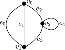
Refer to caption
    Xv0                        Xe2   Xe0   Xe1   Xv2                           Xe4   Xv1                        Xe3    \displaystyle\lx@xy@svg{\hbox{\raise 2.5pt\hbox{\kern 11.63318pt\hbox{\ignorespaces\ignorespaces\ignorespaces\hbox{\vtop{\halign{\entry@#!@&&\entry@@#!@\cr&&&\cr&&&\cr&&&\crcr}}}\ignorespaces{\hbox{\kern-3.0pt\raise 0.0pt\hbox{\hbox{\kern 0.0pt\raise 0.0pt\hbox{\hbox{\kern 3.0pt\raise-2.5pt\hbox{$\textstyle{}$}}}}}}}{\hbox{\kern 35.63318pt\raise 0.0pt\hbox{\hbox{\kern 0.0pt\raise 0.0pt\hbox{\hbox{\kern 3.0pt\raise-2.5pt\hbox{$\textstyle{X_{v_{0}}\ignorespaces\ignorespaces\ignorespaces\ignorespaces\ignorespaces\ignorespaces\ignorespaces\ignorespaces\ignorespaces\ignorespaces\ignorespaces\ignorespaces}$}}}}}}}\ignorespaces\ignorespaces\ignorespaces{}\ignorespaces\ignorespaces{\hbox{\lx@xy@drawline@}}\ignorespaces{\hbox{\kern 11.11455pt\raise-24.0pt\hbox{\hbox{\kern 0.0pt\raise 0.0pt\hbox{\lx@xy@tip{1}\lx@xy@tip{-1}}}}}}\ignorespaces\ignorespaces{\hbox{\lx@xy@drawline@}}\ignorespaces{\hbox{\lx@xy@drawline@}}\ignorespaces\ignorespaces\ignorespaces\ignorespaces{}{\hbox{\lx@xy@droprule}}\ignorespaces{\hbox{\kern 47.4949pt\raise-24.0pt\hbox{\hbox{\kern 0.0pt\raise 0.0pt\hbox{\lx@xy@tip{1}\lx@xy@tip{-1}}}}}}{\hbox{\lx@xy@droprule}}{\hbox{\lx@xy@droprule}}\ignorespaces\ignorespaces\ignorespaces\ignorespaces{}{\hbox{\lx@xy@droprule}}\ignorespaces{\hbox{\kern 83.58517pt\raise 0.0pt\hbox{\hbox{\kern 0.0pt\raise 0.0pt\hbox{\lx@xy@tip{1}\lx@xy@tip{-1}}}}}}{\hbox{\lx@xy@droprule}}{\hbox{\lx@xy@droprule}}{\hbox{\kern 83.58517pt\raise 0.0pt\hbox{\hbox{\kern 0.0pt\raise 0.0pt\hbox{\hbox{\kern 3.0pt\raise-2.5pt\hbox{$\textstyle{X_{e_{2}}}$}}}}}}}{\hbox{\kern 139.71326pt\raise 0.0pt\hbox{\hbox{\kern 0.0pt\raise 0.0pt\hbox{\hbox{\kern 3.0pt\raise-2.5pt\hbox{$\textstyle{}$}}}}}}}{\hbox{\kern-11.63318pt\raise-31.33331pt\hbox{\hbox{\kern 0.0pt\raise 0.0pt\hbox{\hbox{\kern 3.0pt\raise-2.5pt\hbox{$\textstyle{X_{e_{0}}}$}}}}}}}{\hbox{\kern 35.86172pt\raise-31.33331pt\hbox{\hbox{\kern 0.0pt\raise 0.0pt\hbox{\hbox{\kern 3.0pt\raise-2.5pt\hbox{$\textstyle{X_{e_{1}}}$}}}}}}}{\hbox{\kern 83.35663pt\raise-31.33331pt\hbox{\hbox{\kern 0.0pt\raise 0.0pt\hbox{\hbox{\kern 3.0pt\raise-2.5pt\hbox{$\textstyle{X_{v_{2}}\ignorespaces\ignorespaces\ignorespaces\ignorespaces\ignorespaces\ignorespaces\ignorespaces\ignorespaces\ignorespaces\ignorespaces\ignorespaces\ignorespaces\ignorespaces\ignorespaces\ignorespaces\ignorespaces\ignorespaces\ignorespaces}$}}}}}}}\ignorespaces\ignorespaces\ignorespaces\ignorespaces{}{\hbox{\lx@xy@droprule}}\ignorespaces{\hbox{\kern 95.21835pt\raise-8.0pt\hbox{\hbox{\kern 0.0pt\raise 0.0pt\hbox{\lx@xy@tip{1}\lx@xy@tip{-1}}}}}}{\hbox{\lx@xy@droprule}}{\hbox{\lx@xy@droprule}}\ignorespaces\ignorespaces\ignorespaces\ignorespaces{}{\hbox{\lx@xy@droprule}}\ignorespaces{\hbox{\kern 95.21835pt\raise-55.33331pt\hbox{\hbox{\kern 0.0pt\raise 0.0pt\hbox{\lx@xy@tip{1}\lx@xy@tip{-1}}}}}}{\hbox{\lx@xy@droprule}}{\hbox{\lx@xy@droprule}}\ignorespaces\ignorespaces\ignorespaces\ignorespaces\ignorespaces{}{}{}{{}{}{}{}{}{}{}{}{}{}{}{}{}{}{}{}{}{}{}{}{}{}}{}\ignorespaces\hbox{\hbox{\kern 0.0pt\raise 0.0pt\hbox{{}{}{{}}{{}{}{}}{}}}}\ignorespaces{}\ignorespaces{}{}{}{{}{}{}{}{}{}{}{}{}{}{}{}{}{}{}{}{}}{\hbox{\kern 131.08307pt\raise-26.89548pt\hbox{\hbox{\kern 0.0pt\raise 0.0pt\hbox{\lx@xy@tip{1}\lx@xy@tip{-1}}}}}}\ignorespaces\hbox{\hbox{\kern 0.0pt\raise 0.0pt\hbox{{}{}{}{{}}{{}{}{}\lx@xy@spline@}{}}}}\ignorespaces{}\ignorespaces\hbox{\hbox{\kern 0.0pt\raise 0.0pt\hbox{{}{}{{}}{{}{}{}}{}}}}\ignorespaces{}\ignorespaces\ignorespaces\ignorespaces\ignorespaces\ignorespaces{}{}{}{{}{}{}{}{}{}{}{}{}{}{}{}{}{}{}{}{}{}{}{}{}{}}{}\ignorespaces\hbox{\hbox{\kern 0.0pt\raise 0.0pt\hbox{{}{}{{}}{{}{}{}}{}}}}\ignorespaces{}\ignorespaces{}{}{}{{}{}{}{}{}{}{}{}{}{}{}{}{}{}{}{}{}}{\hbox{\kern 131.08307pt\raise-35.77116pt\hbox{\hbox{\kern 0.0pt\raise 0.0pt\hbox{\lx@xy@tip{1}\lx@xy@tip{-1}}}}}}\ignorespaces\hbox{\hbox{\kern 0.0pt\raise 0.0pt\hbox{{}{}{}{{}}{{}{}{}\lx@xy@spline@}{}}}}\ignorespaces{}\ignorespaces\hbox{\hbox{\kern 0.0pt\raise 0.0pt\hbox{{}{}{{}}{{}{}{}}{}}}}\ignorespaces{}{\hbox{\kern 131.08008pt\raise-31.33331pt\hbox{\hbox{\kern 0.0pt\raise 0.0pt\hbox{\hbox{\kern 3.0pt\raise-2.5pt\hbox{$\textstyle{X_{e_{4}}}$}}}}}}}{\hbox{\kern-3.0pt\raise-62.66663pt\hbox{\hbox{\kern 0.0pt\raise 0.0pt\hbox{\hbox{\kern 3.0pt\raise-2.5pt\hbox{$\textstyle{}$}}}}}}}{\hbox{\kern 35.63318pt\raise-62.66663pt\hbox{\hbox{\kern 0.0pt\raise 0.0pt\hbox{\hbox{\kern 3.0pt\raise-2.5pt\hbox{$\textstyle{X_{v_{1}}\ignorespaces\ignorespaces\ignorespaces\ignorespaces\ignorespaces\ignorespaces\ignorespaces\ignorespaces\ignorespaces\ignorespaces\ignorespaces\ignorespaces}$}}}}}}}\ignorespaces\ignorespaces\ignorespaces{}\ignorespaces\ignorespaces{\hbox{\lx@xy@drawline@}}\ignorespaces{\hbox{\kern 11.6332pt\raise-39.00166pt\hbox{\hbox{\kern 0.0pt\raise 0.0pt\hbox{\lx@xy@tip{1}\lx@xy@tip{-1}}}}}}\ignorespaces\ignorespaces{\hbox{\lx@xy@drawline@}}\ignorespaces{\hbox{\lx@xy@drawline@}}\ignorespaces\ignorespaces\ignorespaces\ignorespaces{}{\hbox{\lx@xy@droprule}}\ignorespaces{\hbox{\kern 47.4949pt\raise-39.33331pt\hbox{\hbox{\kern 0.0pt\raise 0.0pt\hbox{\lx@xy@tip{1}\lx@xy@tip{-1}}}}}}{\hbox{\lx@xy@droprule}}{\hbox{\lx@xy@droprule}}\ignorespaces\ignorespaces\ignorespaces\ignorespaces{}{\hbox{\lx@xy@droprule}}\ignorespaces{\hbox{\kern 83.58517pt\raise-62.66663pt\hbox{\hbox{\kern 0.0pt\raise 0.0pt\hbox{\lx@xy@tip{1}\lx@xy@tip{-1}}}}}}{\hbox{\lx@xy@droprule}}{\hbox{\lx@xy@droprule}}{\hbox{\kern 83.58517pt\raise-62.66663pt\hbox{\hbox{\kern 0.0pt\raise 0.0pt\hbox{\hbox{\kern 3.0pt\raise-2.5pt\hbox{$\textstyle{X_{e_{3}}}$}}}}}}}{\hbox{\kern 139.71326pt\raise-62.66663pt\hbox{\hbox{\kern 0.0pt\raise 0.0pt\hbox{\hbox{\kern 3.0pt\raise-2.5pt\hbox{$\textstyle{}$}}}}}}}\ignorespaces}}}}\ignorespaces
Figure A.1: A graph and its associated diagram
Example A.4.

Let ΓM,w\Gamma_{M,w} be the adjacency graph to a matroid subdivision ΔM,w\Delta_{M,w}. Let MvM_{v}, resp. MeM_{e}, denote the matroid corresponding to the vertex vv, resp. edge ee, of ΓM,w\Gamma_{M,w}, and φMv,Me:GrMv,Me\varphi_{M_{v},M_{e}}:\Gr_{M_{v},M_{e}} whenever ee is incident to vv. The data of GrMv,GrMe\Gr_{M_{v}},\Gr_{M_{e}}, and φMv,Me\varphi_{M_{v},M_{e}} defines a diagram of type Q⁡(ΓM,w)Q(\Gamma_{M,w}) in 𝐤-sch\mathop{\mbox{$\mathbf{k}$-$\sch$}}.

Now, let us consider how this construction behaves with respect to contracting a connected subgraph. Let FF be a connected subgraph of GG, and G/FG/F the graph obtained by contracting FF to a single vertex vFv_{F}. Let XF=lim←Q⁡(F)⁡XX_{F}=\varprojlim_{Q(F)}X and ξv:XF→Xv\xi_{v}:X_{F}\to X_{v}, ξe:XF→Xe\xi_{e}:X_{F}\to X_{e} the structure morphisms. Set YvF=XFY_{v_{F}}=X_{F}, and Yv=XvY_{v}=X_{v} for the remaining vv in V⁡(G/F)V(G/F). Similarly, let Ye=XeY_{e}=X_{e} for the edges e∈E⁡(G/F)e\in E(G/F). If hh is a half edge in G/FG/F incident vFv_{F}, set ψh=φh​ξv\psi_{h}=\varphi_{h}\xi_{v}. Otherwise, let ψh=φh\psi_{h}=\varphi_{h}. The data (Yv,Ye,ψh)(Y_{v},Y_{e},\psi_{h}) defines a diagram YY of type Q⁡(G/F)Q(G/F).

Proposition A.5.

We have an isomorphism

lim←G⁡X≅lim←G/F⁡Y.\varprojlim_{G}X\cong\varprojlim_{G/F}Y.
Proof.

To simplify notation, set YG/F=lim←G/F⁡YY_{G/F}=\varprojlim_{G/F}Y. Let λv:YG/F→Yv\lambda_{v}:Y_{G/F}\to Y_{v}, λe:YG/F→Ye\lambda_{e}:Y_{G/F}\to Y_{e} denote the structure morphisms of this limit. We show that YG/FY_{G/F} satisfies the universal property for lim←G⁡X\varprojlim_{G}X. First, we must define morphisms αv:YG/F→Xv\alpha_{v}:Y_{G/F}\to X_{v}, αe:YG/F→Xe\alpha_{e}:Y_{G/F}\to X_{e} that commute with each φh\varphi_{h}. This is achieved by setting αv=ξv​λvF\alpha_{v}=\xi_{v}\lambda_{v_{F}}, (resp. αe=ξe​λvF\alpha_{e}=\xi_{e}\lambda_{v_{F}}) when v∈V⁡(F)v\in V(F) (resp. e∈E⁡(F)e\in E(F)), and αv=λv\alpha_{v}=\lambda_{v}, αe=λe\alpha_{e}=\lambda_{e} otherwise. One may verify that φh​αv=αe\varphi_{h}\alpha_{v}=\alpha_{e}.

Now suppose that we have a collection of morphisms θv:M→Xv\theta_{v}:M\to X_{v} and θe:M→Xe\theta_{e}:M\to X_{e} such that φh​θv=θe\varphi_{h}\theta_{v}=\theta_{e} for every qh:qv→qeq_{h}:q_{v}\to q_{e} in Q⁡(G)Q(G). We will show that there is a unique morphism θ:M→YG/F\theta:M\to Y_{G/F} such that

θ​αv=θv​ and ​θ​αe=θe\theta\alpha_{v}=\theta_{v}\text{ and }\theta\alpha_{e}=\theta_{e} (A.1)

for all v∈V⁡(G)v\in V(G) and e∈E⁡(G)e\in E(G), respectively. By the universal property of XFX_{F}, there is a unique morphism θvF:M→YvF\theta_{v_{F}}:M\to Y_{v_{F}} such that ξv​θvF=θv\xi_{v}\theta_{v_{F}}=\theta_{v} and ξe​θvF=θe\xi_{e}\theta_{v_{F}}=\theta_{e}. If hh is a half edge in G/FG/F incident to vFv_{F}, then

ψh​θvF=φh​ξv​θvF=φh​θv=θe.\psi_{h}\theta_{v_{F}}=\varphi_{h}\xi_{v}\theta_{v_{F}}=\varphi_{h}\theta_{v}=\theta_{e}.

Otherwise, ψh​θv=θe\psi_{h}\theta_{v}=\theta_{e} since ψh=φh\psi_{h}=\varphi_{h}. By the universal property of YG/FY_{G/F}, there is a unique morphism θ:M→YG/F\theta:M\to Y_{G/F} satisfying λv​θ=θv\lambda_{v}\theta=\theta_{v} and λe​θ=θe\lambda_{e}\theta=\theta_{e}.

Now we establish the equalities in Equation A.1. When v∈V⁡(F)v\in V(F),

αv​θ=ξv​λvF​θ=ξv​θvF=θv.\alpha_{v}\theta=\xi_{v}\lambda_{v_{F}}\theta=\xi_{v}\theta_{v_{F}}=\theta_{v}.

A similar argument shows that αe​θ=θe\alpha_{e}\theta=\theta_{e} when e∈E⁡(F)e\in E(F). The cases where v∈V⁡(G)∖V⁡(F)v\in V(G)\setminus V(F) or e∈E⁡(G)∖E⁡(F)e\in E(G)\setminus E(F) follow from the identifications αv=λv\alpha_{v}=\lambda_{v} and αe=λe\alpha_{e}=\lambda_{e}. Finally, the uniqueness of θ\theta follows from the uniqueness of θF\theta_{F} and the universal property of YG/FY_{G/F}. ∎

Proposition A.6.

Suppose GG is a tree, XX a diagram of type Q⁡(G)Q(G) in 𝐤-sch\mathop{\mbox{$\mathbf{k}$-$\sch$}} such XvX_{v} and XeX_{e} are smooth and irreducible 𝐤\mathbf{k}-schemes, and for each half edge hh, X⁡(h):Xv→XeX(h):X_{v}\to X_{e} is a SDC-morphism. Then XGX_{G} is smooth and irreducible. Moreover,

dimXG=∑v∈V⁡(G)Xv−∑e∈E⁡(G)Xe.\dim X_{G}=\sum_{v\in V(G)}X_{v}-\sum_{e\in E(G)}X_{e}.
Proof.

We proceed by induction on the number of vertices. When GG consists of a single vertex, there is nothing to show. Now suppose that the lemma is true for all trees with fewer vertices than GG. Let ww be a one valent vertex of GG, ee the adjacent edge, and G′G^{\prime} the graph consisting of the remaining vertices and edges. By Proposition A.5,

XG≅Xw×XeXG′.X_{G}\cong X_{w}\times_{X_{e}}X_{G^{\prime}}.

It is smooth and irreducible by Proposition A.2 and the inductive hypothesis. Because Xw→XeX_{w}\to X_{e} is smooth of relative dimension dimXw−dimXe\dim X_{w}-\dim X_{e}, so is XG→XG′X_{G}\to X_{G}^{\prime}, and therefore

dimXG=dimXw−dimXe+dimXG′\dim X_{G}=\dim X_{w}-\dim X_{e}+\dim X_{G^{\prime}}

by [15, Corollary 9.6]. By the inductive hypothesis, we get the required formula for dimXG\dim X_{G}. ∎

Remark A.7.

An arbitrary finite limit over a diagram of smooth and irreducible 𝐤\mathbf{k}-schemes in which every morphism is SDC-need not be irreducible. Let h=x2−y2+x+14h=x^{2}-y^{2}+x+\frac{1}{4} and X={Spec}⁡((h)−1​𝐤​[x,y])X=\Spec((h)^{-1}\mathbf{k}[x,y]). Define two morphisms f,g:X→{Spec}⁡𝐤⁡[z]f,g:X\to\Spec\mathbf{k}[z] by:

f#​(z)=x2−y2+x\displaystyle f^{\#}(z)=x^{2}-y^{2}+x g#​(z)=x.\displaystyle g^{\#}(z)=x.

One may verify that ff and gg are SDC-morphisms between smooth and irreducible 𝐤\mathbf{k}-schemes. However, the equalizer of ff and gg is

{Spec}⁡((h)−1​𝐤​[x,y]/⟨x2−y2⟩)\Spec((h)^{-1}\mathbf{k}[x,y]/\langle x^{2}-y^{2}\rangle)

which is neither smooth nor irreducible.

We end with a proposition on when a closed immersion of affine schemes is an isomorphism.

Proposition A.8.

Suppose φ:X↪Y\varphi:X\hookrightarrow Y is a closed immersion of affine schemes, and YY is integral. If dimX=dimY\dim X=\dim Y, then φ\varphi is an isomorphism.

Proof.

Let nn be the Krull dimension of XX and YY. Because φ\varphi is a closed immersion and YY is integral, the induced morphism on rings is of the form φ#:R→R/I\varphi^{\#}:R\to R/I for some integral domain RR and ideal I⊂RI\subset R. A maximal chain of prime ideals 𝔭0⊊𝔭1⊊⋯⊊𝔭n\mathfrak{p}_{0}\subsetneq\mathfrak{p}_{1}\subsetneq\cdots\subsetneq\mathfrak{p}_{n} in R/IR/I lifts to a maximal chain of prime ideals 𝔮0⊊𝔮1⊊⋯⊊𝔮n\mathfrak{q}_{0}\subsetneq\mathfrak{q}_{1}\subsetneq\cdots\subsetneq\mathfrak{q}_{n} in RR with I⊂𝔮0I\subset\mathfrak{q_{0}}. Because RR is an integral domain, 𝔮0=⟨0⟩\mathfrak{q_{0}}=\langle 0\rangle. So I=⟨0⟩I=\langle 0\rangle, and therefore φ#\varphi^{\#} is the identity. ∎

Appendix B Data for Lemma 6.4

In Table B.1, we list the ideals that appear as JM,wxJ_{M,w}^{x} for subdivisions of ΔM,w\Delta_{M,w} such that MM is a simple, connected 𝐤\mathbf{k}-realizable (3,7)(3,7)-matroid and ΓM,w\Gamma_{M,w} has no leaves, as in the proof of Lemma 6.4. We consider all of these as ideals in the ring

𝐤[xi​j±| 0≤i≤2, 0≤j≤3].\mathbf{k}[x_{ij}^{\pm}\ |\ 0\leq i\leq 2,\ 0\leq j\leq 3].

We write 𝐤⁡[xi​j±]\mathbf{k}[x_{ij}^{\pm}] for short. Many of the polynomials that appear are of the form Xi​j,k​ℓ:=xi​k​xj​ℓ−xi​ℓ​xj​kX_{ij,k\ell}:=x_{ik}x_{j\ell}-x_{i\ell}x_{jk}. In the second column, we list variables that may be eliminated to produce an isomorphism of 𝐤⁡[xi​j±]/JM,wx\mathbf{k}[x_{ij}^{\pm}]/J_{M,w}^{x} with a Laurent polynomial ring. For example, consider the last row. In this case,

JM,wx=⟨X01,23,X02,03,X12,12,X12,02,X12,01⟩.J_{M,w}^{x}=\langle X_{01,23},X_{02,03},X_{12,12},X_{12,02},X_{12,01}\rangle.

We use X01,23X_{01,23} to solve for x02x_{02}, X02,03X_{02,03} for x03x_{03}, X12,12X_{12,12} for x11x_{11}, and finally X12,02X_{12,02} for x22x_{22}. This produces an isomorphism 𝐤[xi​j±]/JM,wx→𝐤[xi​j±|ij≠02,03,11,22]\mathbf{k}[x_{ij}^{\pm}]/J_{M,w}^{x}\to\mathbf{k}[x_{ij}^{\pm}\,|\,ij\neq 02,03,11,22].

Ideals xi​jx_{ij} to eliminate
X12,01\!X_{12,01} x21x_{21}
X01,12\!X_{01,12} x12x_{12}
X12,12\!X_{12,12} x22x_{22}
X02,23\!X_{02,23} x23x_{23}
X01,03\!X_{01,03} x13x_{13}
X01,23\!X_{01,23} x13x_{13}
X12,23\!X_{12,23} x23x_{23}
X01,02\!X_{01,02} x12x_{12}
x02​x10​x21+x00​x11​x22\!x_{02}x_{10}x_{21}+x_{00}x_{11}x_{22} x22x_{22}
x00​x12​x21+x01​x10​x22\!x_{00}x_{12}x_{21}+x_{01}x_{10}x_{22} x22x_{22}
x00​x13​x22+x02​x10​x23\!x_{00}x_{13}x_{22}+x_{02}x_{10}x_{23} x23x_{23}
x02​x10​x21−x00​x12​x21−x01​x10​x22\!x_{02}x_{10}x_{21}-x_{00}x_{12}x_{21}-x_{01}x_{10}x_{22} x22x_{22}
x02​x11​x20−x01​x12​x20−x00​x11​x22\!x_{02}x_{11}x_{20}-x_{01}x_{12}x_{20}-x_{00}x_{11}x_{22} x22x_{22}
x03​x10​x22−x00​x13​x22−x02​x10​x23\!x_{03}x_{10}x_{22}-x_{00}x_{13}x_{22}-x_{02}x_{10}x_{23} x23x_{23}
x03​x10​x22−x00​x13​x22+x00​x12​x23\!x_{03}x_{10}x_{22}-x_{00}x_{13}x_{22}+x_{00}x_{12}x_{23} x23x_{23}
x02​x10​x21−x00​x12​x21−x01​x10​x22+x00​x11​x22\!x_{02}x_{10}x_{21}-x_{00}x_{12}x_{21}-x_{01}x_{10}x_{22}+x_{00}x_{11}x_{22} x11x_{11}
X02,23,X12,01\!X_{02,23},X_{12,01} x21,x23x_{21},x_{23}
X02,02,X12,01\!X_{02,02},X_{12,01} x21,x22x_{21},x_{22}
X01,03,X12,01\!X_{01,03},X_{12,01} x13,x21x_{13},x_{21}
X02,03,X12,01\!X_{02,03},X_{12,01} x21,x23x_{21},x_{23}
X02,13,X01,02\!X_{02,13},X_{01,02} x12,x23x_{12},x_{23}
X02,12,X12,01\!X_{02,12},X_{12,01} x01,x22x_{01},x_{22}
X02,13,X12,01\!X_{02,13},X_{12,01} x10,x23x_{10},x_{23}
X01,13,X01,02\!X_{01,13},X_{01,02} x12,x13x_{12},x_{13}
X12,13,x00​x12​x21+x01​x10​x22\!X_{12,13},x_{00}x_{12}x_{21}+x_{01}x_{10}x_{22} x22,x23x_{22},x_{23}
X01,13,x02​x10​x21−x00​x12​x21−x01​x10​x22\!X_{01,13},x_{02}x_{10}x_{21}-x_{00}x_{12}x_{21}-x_{01}x_{10}x_{22} x13,x22x_{13},x_{22}
X12,13,x02​x10​x21−x01​x10​x22+x00​x11​x22\!X_{12,13},x_{02}x_{10}x_{21}-x_{01}x_{10}x_{22}+x_{00}x_{11}x_{22} x02,x23x_{02},x_{23}
X01,12,x03​x10​x22−x00​x13​x22−x02​x10​x23\!X_{01,12},x_{03}x_{10}x_{22}-x_{00}x_{13}x_{22}-x_{02}x_{10}x_{23} x12,x23x_{12},x_{23}
X02,03,X01,12,X12,01\!X_{02,03},X_{01,12},X_{12,01} x12,x21,x23x_{12},x_{21},x_{23}
X01,13,X02,02,X12,01\!X_{01,13},X_{02,02},X_{12,01} x13,x22,x21x_{13},x_{22},x_{21}
X02,13,X02,02,X12,01\!X_{02,13},X_{02,02},X_{12,01} x10,x22,x23x_{10},x_{22},x_{23}
X12,12,X12,02,X12,01\!X_{12,12},X_{12,02},X_{12,01} x22,x21x_{22},x_{21}
X12,03,X01,23,x02​x11​x20+x01​x10​x22−x00​x11​x22\!X_{12,03},X_{01,23},x_{02}x_{11}x_{20}+x_{01}x_{10}x_{22}-x_{00}x_{11}x_{22} x00,x12,x23x_{00},x_{12},x_{23}
X01,03,X02,02,−X12,01−x02​x13​x21+x03​x11​x22\!X_{01,03},X_{02,02},-X_{12,01}-x_{02}x_{13}x_{21}+x_{03}x_{11}x_{22} x00,x01,x13x_{00},x_{01},x_{13}
X02,03,X12,12,X12,02,X12,01\!X_{02,03},X_{12,12},X_{12,02},X_{12,01} x11,x22,x23x_{11},x_{22},x_{23}
X02,13,X01,12,X12,01,x03​x12​x20−x02​x10​x23\!X_{02,13},X_{01,12},X_{12,01},x_{03}x_{12}x_{20}-x_{02}x_{10}x_{23} x12,x21,x23x_{12},x_{21},x_{23}
X02,02,X12,01,x01​x13​x22+x02​x11​x23,x01​x13​x20+x00​x11​x23\!X_{02,02},X_{12,01},x_{01}x_{13}x_{22}+x_{02}x_{11}x_{23},x_{01}x_{13}x_{20}+x_{00}x_{11}x_{23}\! x00,x10,x22x_{00},x_{10},x_{22}
X12,23,X02,13,X02,02,X12,01,\!X_{12,23},X_{02,13},X_{02,02},X_{12,01}, x00,x13,x20,x22,x_{00},x_{13},x_{20},x_{22},\!
x00​x03​x11​x12−x01​x02​x10​x13x_{00}x_{03}x_{11}x_{12}-x_{01}x_{02}x_{10}x_{13} x23x_{23}
X01,23,X02,03,X12,12,X12,02,X12,01\!X_{01,23},X_{02,03},X_{12,12},X_{12,02},X_{12,01} x02,x03,x11,x22x_{02},x_{03},x_{11},x_{22}\!
Table B.1: Here are the unique ideals nontrivial ideals that appear in the proof of Lemma 6.4

Appendix C Maps between thin Schubert cells and inverse limits (written by María Angélica Cueto)

In this appendix, we discuss how to reduce the study of geometric properties of thin Schubert cells to the case of simple and connected matroids. Because the only simple rank 2 matroid is U⁡(2,n)U(2,n), this analysis gives us a complete understanding of GrM\Gr_{M} in the rank 2 case, and simplifies the study of rank 33 matroids in Sections 4 and 5. In the following subsection, we show that the limit of thin Schubert cell GrM,w\Gr_{M,w} induced by a matroid subdivision ΔM,w\Delta_{M,w} depends only on the adjacency graph of ΔM,w\Delta_{M,w}. This allows one to apply the results from Appendix A to study GrM,w\Gr_{M,w} as in Section 6.

C.1 Reduction to simple and connected matroids

The following two Lemmas demonstrate that thin Schubert cells are compatible with decomposition into connected components and removal of loops and parallel elements. Lemma C.1 appears [21, Proposition 9.4] without proof, and Lemma C.2 will appear in an upcoming paper [4]. For the reader’s convenience, we sketch their proofs.

Lemma C.1.

If M=M1⊕M2M=M_{1}\oplus M_{2}, then GrM≅GrM1×GrM2\Gr_{M}\cong\Gr_{M_{1}}\times\Gr_{M_{2}}. In particular, GrM≅GrM|T\Gr_{M}\cong\Gr_{M|T} where T⊂[n]T\subset[n] is the set of non-loop elements.

Proof.

Suppose X1X_{1} and X2X_{2} are matrices giving rise to the rings RM1xR_{M_{1}}^{x}, RM2xR_{M_{2}}^{x} as in Construction 2.2. Let XX be the block matrix with X1X_{1} and X2X_{2} on the diagonal. Then RMx≅RM1x⊗RM2xR_{M}^{x}\cong R_{M_{1}}^{x}\otimes R_{M_{2}}^{x}. The second statement follow from M≅M|T⊕U⁡(0,|T|)M\cong M|T\oplus U(0,|T|). ∎

Given a matroid MM, we define a simple matroid by removing loops and parallel elements in the following way. Let η1,…,ηk\eta_{1},\ldots,\eta_{k} be the rank 1 flats of MM, choose nonloop elements si∈ηis_{i}\in\eta_{i} and set S={s1,…,sk}S=\{s_{1},\ldots,s_{k}\}. Then M|SM|S is a simple matroid. Let ℓ\ell be the number of loops in MM.

Lemma C.2.

We have an isomorphism GrM≅GrM|S×𝔾mn−k−ℓ\Gr_{M}\cong\Gr_{M|S}\times{\mathbb{G}}_{m}^{n-k-\ell}.

Proof.

By Lemma C.1, we may assume that MM has no loops. Suppose i,ji,j are parallel in MM, then GrM≅GrM[n]∖i×𝔾m\Gr_{M}\cong\Gr_{M_{[n]\setminus i}}\times{\mathbb{G}}_{m}. Suppose ii and jj are parallel, and let μ1,μ2∈([n]d−1)\mu_{1},\mu_{2}\in{[n]\choose d-1} such that μk∪{i}\mu_{k}\cup\{i\} and μk∪{j}\mu_{k}\cup\{j\} are bases of MM for k=1,2k=1,2. The quadratic generator from Equation 3.1 yields

PM​(μ1∪{i,j},μ2)=pμ1∪i​pμ2∪j−pμ1∪j​pμ2∪iP_{M}(\mu_{1}\cup\{i,j\},\mu_{2})=p_{\mu_{1}\cup i}p_{\mu_{2}\cup j}-p_{\mu_{1}\cup j}p_{\mu_{2}\cup i}

This means that pμ∪i/pμ∪jp_{\mu\cup i}/p_{\mu\cup j} is independent of μ\mu. At the level of rings, the desired isomorphism RM[n]∖i⊗𝐤⁡[t±]≅RMR_{M_{[n]\setminus i}}\otimes\mathbf{k}[t^{\pm}]\cong R_{M} is given by

RM[n]∖i⊗𝐤⁡[t±]\displaystyle R_{M_{[n]\setminus i}}\otimes\mathbf{k}[t^{\pm}] ⟶RM\displaystyle\longrightarrow R_{M}
pλ⊗1\displaystyle p_{\lambda}\otimes 1 ↦pλ if ​i∉λ,\displaystyle\mapsto p_{\lambda}\;\;\;\;\;\;\;\;\;\;\;\;\;\;\;\text{ if }i\notin\lambda,
1⊗t\displaystyle 1\otimes t ↦pμ∪i/pμ∪j if ​λ=μ∪{i}.\displaystyle\mapsto p_{\mu\cup i}/p_{\mu\cup j}\;\;\;\;\text{ if }\lambda=\mu\cup\{i\}.

The Lemma now follows by induction on the number of parallel elements in MM. ∎

Because the uniform matroid U⁡(2,n)U(2,n) is the only simple (2,[n])(2,[n])-matroid, and affine coordinates realize Gr0⁡(2,n)\Gr_{0}(2,n) as a open subscheme of an algebraic torus, we have the following.

Proposition C.3.

If MM is a rank 2 matroid then

GrM≅Gr0⁡(2,k)×𝔾mn−k−ℓ.\Gr_{M}\cong\Gr_{0}(2,k)\times{\mathbb{G}}_{m}^{n-k-\ell}. (C.1)

where kk is the number of rank 1 flats and ℓ\ell the number of loops. In particular, GrM\Gr_{M} is smooth and irreducible.

Next, we show the morphisms φM,M′:GrM→GrM′\varphi_{M,M^{\prime}}:\Gr_{M}\to\Gr_{M^{\prime}} are compatible with the following operations: decomposition of matroids into connected components, removal of loops and parallel elements, and duality. This will allow us to restrict our attention to pairs M′≤MM^{\prime}\leq M where MM is simple, connected, and d=rM​([n])≤⌊n/2⌋d=r_{M}([n])\leq\lfloor n/2\rfloor.

Lemma C.4.

If M′≤MM^{\prime}\leq M and M=M1⊕M2M=M_{1}\oplus M_{2}, then M′=M1′⊕M2′M^{\prime}=M^{\prime}_{1}\oplus M^{\prime}_{2} with Mi′≤MiM^{\prime}_{i}\leq M_{i} for i=1,2i=1,2. Furthermore, φM,M′=φM1,M1′×φM2,M2′\varphi_{M,M^{\prime}}=\varphi_{M_{1},M^{\prime}_{1}}\times\varphi_{M_{2},M^{\prime}_{2}}.

Proof.

Recall that ΔM=ΔM1×ΔM2\Delta_{M}=\Delta_{M_{1}}\times\Delta_{M_{2}} if and only if M=M1⊕M2M=M_{1}\oplus M_{2}. Thus, a face of ΔM\Delta_{M} must be of the form ΔM1′×ΔM2′\Delta_{M_{1}^{\prime}}\times\Delta_{M_{2}^{\prime}} for Mi′≤MiM_{i}^{\prime}\leq M_{i} for i=1,2i=1,2 so M′=M1′⊕M2′M^{\prime}=M_{1}^{\prime}\oplus M_{2}^{\prime}. The statement regarding φM,M′\varphi_{M,M^{\prime}} follows by combining this decomposition with Proposition 3.2 and Lemma C.1. ∎

Lemma C.5.

If M′≤MM^{\prime}\leq M, then we have M′|S≤M|SM^{\prime}|S\leq M|S and the restrictions fit into the commutative diagram:

    GrM    ≅          φM,M′         GrM|S×𝔾mn−k−ℓ    φM|S,M′|S×i​d         GrM′    ≅         GrM′|S×𝔾mn−k−ℓ.    \displaystyle\lx@xy@svg{\hbox{\raise 2.55554pt\hbox{\kern 30.06198pt\hbox{\ignorespaces\ignorespaces\ignorespaces\hbox{\vtop{\halign{\entry@#!@&&\entry@@#!@\cr&\cr&\crcr}}}\ignorespaces{\hbox{\kern-13.76413pt\raise 0.0pt\hbox{\hbox{\kern 0.0pt\raise 0.0pt\hbox{\hbox{\kern 3.0pt\raise-2.55554pt\hbox{$\textstyle{\Gr_{M}\ignorespaces\ignorespaces\ignorespaces\ignorespaces\ignorespaces\ignorespaces\ignorespaces\ignorespaces}$}}}}}}}\ignorespaces\ignorespaces\ignorespaces\ignorespaces{}{\hbox{\lx@xy@droprule}}\ignorespaces\ignorespaces\ignorespaces{\hbox{\kern 22.186pt\raise 6.15pt\hbox{{}\hbox{\kern 0.0pt\raise 0.0pt\hbox{\hbox{\kern 3.0pt\hbox{\hbox{\kern 0.0pt\raise-1.75pt\hbox{$\scriptstyle{\cong}$}}}\kern 3.0pt}}}}}}\ignorespaces{\hbox{\kern 41.8579pt\raise 0.0pt\hbox{\hbox{\kern 0.0pt\raise 0.0pt\hbox{\lx@xy@tip{1}\lx@xy@tip{-1}}}}}}{\hbox{\lx@xy@droprule}}{\hbox{\lx@xy@droprule}}\ignorespaces\ignorespaces\ignorespaces\ignorespaces{}{\hbox{\lx@xy@droprule}}\ignorespaces\ignorespaces\ignorespaces{\hbox{\kern-30.06198pt\raise-16.46724pt\hbox{{}\hbox{\kern 0.0pt\raise 0.0pt\hbox{\hbox{\kern 3.0pt\hbox{\hbox{\kern 0.0pt\raise-0.11528pt\hbox{$\scriptstyle{\varphi_{M,M^{\prime}}}$}}}\kern 3.0pt}}}}}}\ignorespaces{\hbox{\kern 0.0pt\raise-25.65671pt\hbox{\hbox{\kern 0.0pt\raise 0.0pt\hbox{\lx@xy@tip{1}\lx@xy@tip{-1}}}}}}{\hbox{\lx@xy@droprule}}{\hbox{\lx@xy@droprule}}{\hbox{\kern 41.8579pt\raise 0.0pt\hbox{\hbox{\kern 0.0pt\raise 0.0pt\hbox{\hbox{\kern 3.0pt\raise-2.55554pt\hbox{$\textstyle{\Gr_{M|S}\times{\mathbb{G}}_{m}^{n-k-\ell}\ignorespaces\ignorespaces\ignorespaces\ignorespaces}$}}}}}}}\ignorespaces\ignorespaces\ignorespaces\ignorespaces{}{\hbox{\lx@xy@droprule}}\ignorespaces\ignorespaces\ignorespaces{\hbox{\kern 76.5684pt\raise-16.46724pt\hbox{{}\hbox{\kern 0.0pt\raise 0.0pt\hbox{\hbox{\kern 3.0pt\hbox{\hbox{\kern 0.0pt\raise-0.9pt\hbox{$\scriptstyle{\varphi_{M|S,M^{\prime}|S}\times id}$}}}\kern 3.0pt}}}}}}\ignorespaces{\hbox{\kern 76.5684pt\raise-24.0pt\hbox{\hbox{\kern 0.0pt\raise 0.0pt\hbox{\lx@xy@tip{1}\lx@xy@tip{-1}}}}}}{\hbox{\lx@xy@droprule}}{\hbox{\lx@xy@droprule}}{\hbox{\kern-15.11656pt\raise-32.93448pt\hbox{\hbox{\kern 0.0pt\raise 0.0pt\hbox{\hbox{\kern 3.0pt\raise-2.55554pt\hbox{$\textstyle{\Gr_{M^{\prime}}\ignorespaces\ignorespaces\ignorespaces\ignorespaces}$}}}}}}}\ignorespaces\ignorespaces\ignorespaces\ignorespaces{}{\hbox{\lx@xy@droprule}}\ignorespaces\ignorespaces\ignorespaces{\hbox{\kern 21.49156pt\raise-26.78448pt\hbox{{}\hbox{\kern 0.0pt\raise 0.0pt\hbox{\hbox{\kern 3.0pt\hbox{\hbox{\kern 0.0pt\raise-1.75pt\hbox{$\scriptstyle{\cong}$}}}\kern 3.0pt}}}}}}\ignorespaces{\hbox{\kern 39.11656pt\raise-32.93448pt\hbox{\hbox{\kern 0.0pt\raise 0.0pt\hbox{\lx@xy@tip{1}\lx@xy@tip{-1}}}}}}{\hbox{\lx@xy@droprule}}{\hbox{\lx@xy@droprule}}{\hbox{\kern 39.11656pt\raise-32.93448pt\hbox{\hbox{\kern 0.0pt\raise 0.0pt\hbox{\hbox{\kern 3.0pt\raise-2.55554pt\hbox{$\textstyle{\Gr_{M^{\prime}|S}\times{\mathbb{G}}_{m}^{n-k-\ell}.}$}}}}}}}\ignorespaces}}}}\ignorespaces (C.2)
Proof.

The top horizontal map in (C.2) arises from the isomorphism GrM≃GrM|S×𝔾mn−k−ℓ\Gr_{M}\simeq\Gr_{M|S}\times{\mathbb{G}}_{m}^{n-k-\ell} described in Lemma C.2. Since M′≤MM^{\prime}\leq M, rank-one flats in MM yield rank-one flats in M′M^{\prime} we have M′|S≤M|SM^{\prime}|S\leq M|S. The same lemma yields GrM≅GrM′|S×𝔾mn−k−ℓ\Gr_{M}\cong\Gr_{M^{\prime}|S}\times{\mathbb{G}}_{m}^{n-k-\ell}. This determines the bottom horizontal map. ∎

Now we ensure the compatibility of M′≤MM^{\prime}\leq M with the duality operation and the isomorphism

ψ:Gr⁡(d,n)→Gr⁡(n−d,n)(pβ)β↦((−1)sign⁡(β,βc)​pβc)βc\psi:\Gr(d,n)\to\Gr(n-d,n)\hskip 10.0pt(p_{\beta})_{\beta}\mapsto((-1)^{\operatorname{sign}(\beta,\beta^{c})}p_{\beta^{c}})_{\beta^{c}}

induced from ℙ(∧d𝐤n)≅ℙ(∧n−d𝐤n)\mathbb{P}(\wedge^{d}\mathbf{k}^{n})\cong\mathbb{P}(\wedge^{n-d}\mathbf{k}^{n}). Here, (β,βc)(\beta,\beta^{c}) is a permutation of SnS_{n} in one-line notation and βc=[n]∖β\beta^{c}=[n]\smallsetminus\beta. On affine patches, the correspondence for matrices is explicit: for example, a d×nd\times n matrix (Id|X)(I_{d}|X) in {p[d]≠0}\{p_{[d]}\neq 0\} is identified with the (n−d)×n(n-d)\times n matrix (−Xt|In−d)(-X^{t}|I_{n-d}) in {p[d]c≠0}\{p_{[d]^{c}}\neq 0\}.

Lemma C.6.

If M′≤MM^{\prime}\leq M then (M′)∗≤M∗(M^{\prime})^{*}\leq M^{*} and φM∗,(M′)∗=ψ∘φM,M′∘ψ−1\varphi_{M^{*},(M^{\prime})^{*}}=\psi\circ\varphi_{M,M^{\prime}}\circ\psi^{-1}.

Proof.

By definition, ΔM∗=conv⁡({𝟏−eβ:β∈B⁡(M)})=𝟏−ΔM\Delta_{M^{*}}=\conv(\{\mathbf{1}-e_{\beta}\colon\beta\in{\pazocal B}(M)\})=\mathbf{1}-\Delta_{M}. In particular, if ΔM′\Delta_{M^{\prime}} is a face of ΔM\Delta_{M}, then Δ(M′)∗=(𝟏−ΔM′)≺(𝟏−ΔM)=ΔM∗\Delta_{(M^{\prime})^{*}}=(\mathbf{1}-\Delta_{M^{\prime}})\prec(\mathbf{1}-\Delta_{M})=\Delta_{M^{*}}, as required. The isomorphism ψ\psi identifies each pβ∈𝐤⁡[Gr⁡(d,n)]p_{\beta}\in\mathbf{k}[\Gr(d,n)] with pβc∈𝐤⁡[Gr⁡(n−d,n)]p_{\beta^{c}}\in\mathbf{k}[\Gr(n-d,n)]. The expression φM∗,(M′)∗=ψ∘φM,M′∘ψ−1\varphi_{M^{*},(M^{\prime})^{*}}=\psi\circ\varphi_{M,M^{\prime}}\circ\psi^{-1} follows from this observation. ∎

As an application, we prove that φM,M′\varphi_{M,M^{\prime}} is a SDC-morphism whenever M=U⁡(d,n)M=U(d,n) or MM is a rank 22 matroid.

Proposition C.7.

For any M′≤M:=U⁡(d,n)M^{\prime}\leq M:=U(d,n), the map φM,M′:Gr0⁡(d,n)→GrM′\varphi_{M,M^{\prime}}\colon\Gr_{0}(d,n)\to\Gr_{M^{\prime}} is a SDC-morphism.

Proof.

By Proposition A.3, it suffices to show that φM,M′\varphi_{M,M^{\prime}} is a SDC morphism when M′⋖MM^{\prime}\lessdot M. The nondegenerate subsets of MM are of the form {i}\{i\} or [n]∖i[n]\setminus i for some i∈[n]i\in[n]. If M′=M{i}M^{\prime}=M_{\{i\}}, then (M′)∗=M[n]∖i∗(M^{\prime})^{*}=M^{*}_{[n]\setminus i} where M∗≅U⁡(n−d,n)M^{*}\cong U(n-d,n). By Lemma C.6, it suffices to consider just M′=M[n]∖{i}M^{\prime}=M_{[n]\setminus\{i\}}. In this case, RM′x=(SM′x)−1​BM′R_{M^{\prime}}^{x}=(S_{M^{\prime}}^{x})^{-1}B_{M^{\prime}} and RM′x=(SMx)−1​RM′x​[xi,n−4±|i∈[d]]R_{M^{\prime}}^{x}=(S_{M}^{x})^{-1}R_{M^{\prime}}^{x}[x_{i,n-4}^{\pm}\,|\,i\in[d]\,]. Therefore GrM⊂𝔾md×(n−d)\Gr_{M}\subset{\mathbb{G}}_{m}^{d\times(n-d)}, GrM⊂𝔾md×(n−d−1)\Gr_{M}\subset{\mathbb{G}}_{m}^{d\times(n-d-1)} as open subvarieties, and φM,M′\varphi_{M,M^{\prime}} is induced by a coordinate projection 𝔾md×(n−d)→𝔾md×(n−d−1){\mathbb{G}}_{m}^{d\times(n-d)}\to{\mathbb{G}}_{m}^{d\times(n-d-1)}, which is clearly a SDC-morphism. The result now follows from A.3. ∎

Proposition C.8.

For (2,[n])(2,[n])-matroids M′≤MM^{\prime}\leq M, φM,M′\varphi_{M,M^{\prime}} is a SDC morphism.

Proof.

Because every simple rank 22 matroid is uniform, the Proposition follows from Lemmas C.4, C.5, and C.7. ∎

Our final result in this subsection say that the reduction to simple matroids as above is compatible taking initial degenerations and inverse limits.

Proposition C.9.

Fix w∈TGrMw\in\TGr_{M} and let w~\tilde{w} be the projection of ww to ℝB⁡(M|S)/ℝ⋅𝟏{\mathbb{R}}^{{\pazocal B}(M|S)}/{\mathbb{R}}\!\cdot\!\mathbf{1}. Then w~∈TGrM|S\tilde{w}\in\TGr_{M|S} and

inw⁡GrM≃inw~⁡GrM|S×𝔾mn−k−ℓ\displaystyle\operatorname{in}_{w}\Gr_{M}\simeq\operatorname{in}_{\tilde{w}}\Gr_{M|S}\times{\mathbb{G}}_{m}^{n-k-\ell} GrM,w≅GrM|S,w~×𝔾mn−k−ℓ\displaystyle\Gr_{M,w}\cong\Gr_{M|S,\tilde{w}}\times{\mathbb{G}}_{m}^{n-k-\ell}
Proof.

The assertion on initial degenerations follows from the fact that the isomorphism GrM≅GrM|S×𝔾mn−k−ℓ\Gr_{M}\cong\Gr_{M|S}\times{\mathbb{G}}_{m}^{n-k-\ell} from Lemma C.2 is induced by a monomial map on coordinate rings. The isomorphism of limits follows from this Lemma and the description of the coordinate ring of GrM,w\Gr_{M,w} in Proposition 3.7. ∎

C.2 Limits of thin Schubert cells via adjacency graphs

Recall that the matroid subdivision ΔM,w\Delta_{M,w} yields a system of maps φMQ,MQ′:GrMQ→GrMQ′\varphi_{M_{Q},M_{Q^{\prime}}}:\Gr_{M_{Q}}\to\Gr_{M_{Q^{\prime}}} whenever Q′≤QQ^{\prime}\leq Q that satisfy φMQ,MQ′′=φMQ′,MQ′′​φMQ,MQ′\varphi_{M_{Q},M_{Q^{\prime\prime}}}=\varphi_{M_{Q^{\prime}},M_{Q^{\prime\prime}}}\varphi_{M_{Q},M_{Q^{\prime}}} and φMQ,MQ=id\varphi_{M_{Q},M_{Q}}=\id. This allows us to form the limit

GrM,w:=lim⟵MQ∈ΔM,wGrMQ\Gr_{M,w}:=\lim_{\begin{subarray}{c}\longleftarrow\\ M_{Q}\in\Delta_{M,w}\end{subarray}}\Gr_{M_{Q}} (C.3)

Rather than keeping track of the full face poset of ΔM,w\Delta_{M,w} it is desirable to restrict ourselves to cells of codimension 0 and 1. The following construction mimics the definition of adjacency graphs for triangulations of polytopes [5, Definition 4.5.10], so we use the same name.

Definition C.10.

Given ww in DrM\operatorname{Dr}_{M}, let ΓM,w\Gamma_{M,w} be the adjacency graph of ΔM,w\Delta_{M,w} defined as follows. The graph ΓM,w\Gamma_{M,w} has a vertex vQv_{Q} for each QQ in TCM,w\operatorname{TC}_{M,w}. Two vertices vQ1,vQ2v_{Q_{1}},v_{Q_{2}} are connected by an edge if Q1∩Q2Q_{1}\cap Q_{2} is a facet of both cells. Similarly, given a cell FF of ΔM,w\Delta_{M,w}, we let ΓM,wF\Gamma_{M,w}^{F} be the full subgraph of ΓM,w\Gamma_{M,w} generated by those vertices vQv_{Q} of ΓM,w\Gamma_{M,w} with F≤QF\leq Q.

Our next lemma shows that the graphs defined above are connected. It will play a crucial role in C.12 below.

Lemma C.11.

For any w∈DrMw\in\operatorname{Dr}_{M} and any cell FF of ΔM,w\Delta_{M,w}, the graphs ΓM,w\Gamma_{M,w} and ΓM,wF\Gamma_{M,w}^{F} are connected.

Proof.

The first claim follows by convexity and is valid for the adjacency graph associated to a pure-dimensional polyhedral subdivision of any polytope. We argue for ΔM\Delta_{M} and ΔM,w\Delta_{M,w}. Indeed, given two vertices vQ1,vQ2v_{Q_{1}},v_{Q_{2}} of ΓM,w\Gamma_{M,w}, choose two points x1,x2x_{1},x_{2}, with xi∈rel​int⁡(Qi)x_{i}\in\operatorname{rel\,int}(Q_{i}) so that the segment [x1,x2][x_{1},x_{2}] does not meet any cell whose codimension is 22 or greater. Since ΔM\Delta_{M} is convex, the [x1,x2][x_{1},x_{2}] lies in rel​int⁡(ΔM)\operatorname{rel\,int}(\Delta_{M}). All but finitely many points in [x1,x2][x_{1},x_{2}] lie in the relative interior of top-dimensional cells. We label the encountered cells as we move from x1x_{1} towards x2x_{2} by Q1=:Q0′,Q1′,…,Qk′:=Q2Q_{1}=:\!Q^{\prime}_{0},Q^{\prime}_{1},\ldots,Q^{\prime}_{k}\!:=Q_{2}. The collection {Qi′}i\{Q^{\prime}_{i}\}_{i} yields a path from vQ1v_{Q_{1}} to vQ2v_{Q_{2}} in ΓM,w\Gamma_{M,w}.

A similar argument can be used to prove the statement for ΓM,wF\Gamma_{M,w}^{F}. Let E⊂ℝnE\subset{\mathbb{R}}^{n} be the affine span of ΔM\Delta_{M}. Given FF in ΔM,w\Delta_{M,w}, write s:=dimFs:=\dim F and pick a point pp in its relative interior. We let HH be the orthogonal complement to the linear subspace F−pF-p in E−pE-p, and QQ a (m−s)(m-s)-dimensional cube in HH centered at the origin with diameter 0<ε≪10<\varepsilon\ll 1.

We consider the full-dimensional polytope P′:=(Q+p)∩ΔMP^{\prime}:=(Q+p)\cap\Delta_{M} in H+pH+p, and the polyhedral subdivision on P′P^{\prime} induced by ΔM,w\Delta_{M,w}. Each cell in this subdivision equals Q′∩ΔMQ^{\prime}\cap\Delta_{M} for some Q′Q^{\prime}, and has dimension (s−dimΔM+dimQ)(s-\dim\Delta_{M}+\dim Q). By construction, a matroid polytope Q′Q^{\prime} yields a vertex or edge of ΓM,wF\Gamma_{M,w}^{F} if and only if Q′∈ΔM,wQ^{\prime}\in\Delta_{M,w} and Q′∩(Q+p)≠∅Q^{\prime}\cap(Q+p)\neq\emptyset. Thus, ΓM,w\Gamma_{M,w} agrees with the adjacency graph of the subdivision of P′P^{\prime}. Since the latter is connected by the discussion above, the result follows. ∎

The adjacency graph ΓM,w\Gamma_{M,w} encodes a subsystem of the inverse system GrM,w\Gr_{M,w} from (C.3) as in Example A.4. Our final result shows that GrM,w\Gr_{M,w} agrees with the inverse system induced by ΓM,w\Gamma_{M,w}.

Proposition C.12.

Let MM be a 𝐤\mathbf{k}-realizable (d,[n])(d,[n])-matroid and w∈TGrMw\in\TGr_{M}. Then,

GrM,w≅lim←ΓM,w⁡GrM′.\Gr_{M,w}\cong\varprojlim_{\Gamma_{M,w}}\Gr_{M^{\prime}}. (C.4)
Proof.

We write GrM,wΓ\Gr_{M,w}^{\Gamma} for the inverse limit on the right-hand side of Equation C.4. Given M′M^{\prime} labeling a cell of ΓM,w\Gamma_{M,w}, we write hM′Γ:GrM,wΓ→GrM′h_{M^{\prime}}^{\Gamma}\colon\Gr_{M,w}^{\Gamma}\to\Gr_{M^{\prime}} for the associated morphism. Since ΓM,w\Gamma_{M,w} determines a subsystem of ΔM,w\Delta_{M,w}, the universal property of GrM,wΓ\Gr_{M,w}^{\Gamma} guarantees the existence of a morphism ψ:GrM,w→GrM,wΓ\psi:\Gr_{M,w}\to\Gr_{M,w}^{\Gamma}. Next, we build a morphism ϕ:GrM,wΓ→GrM,w\phi:\Gr_{M,w}^{\Gamma}\to\Gr_{M,w}.

First, we construct morphisms gF:GrM,wΓ→GrFg_{F}\colon\Gr_{M,w}^{\Gamma}\to\Gr_{F} for each cell ΔF\Delta_{F} of ΔM,w\Delta_{M,w}, satisfying gM′′=φM′,M′′∘gM′g_{M^{\prime\prime}}=\varphi_{M^{\prime},M^{\prime\prime}}\circ g_{M^{\prime}} for each pair of cells in ΔM,w\Delta_{M,w} with M′≤M′′M^{\prime}\leq M^{\prime\prime}. The morphism ϕ\phi will be unique determined once we establish the compatibility of all gFg_{F}’s with the subdivision ΔM,w\Delta_{M,w}.

Let 𝒱F\mathscr{V}_{F} be the set of vertices of the graph ΓM,wF\Gamma_{M,w}^{F}. Set gF:=φM′,F∘hM′Γg_{F}:=\varphi_{M^{\prime},F}\circ h_{M^{\prime}}^{\Gamma} where vM′∈𝒱Fv_{M^{\prime}}\in\mathscr{V}_{F}. We must show this morphism is independent of our choice of M′M^{\prime}. Suppose vM′′∈VFv_{M^{\prime\prime}}\in V_{F} as well. Since ΓM,wF\Gamma_{M,w}^{F} is connected by C.11, we can find a collection of vertices vQM′=:vQ0,vQ1,…,vQk:=vQM′′v_{Q_{M^{\prime}}}=:\!v_{Q_{0}},v_{Q_{1}},\ldots,v_{Q_{k}}\!:=v_{Q_{M^{\prime\prime}}} where (vQi,vQi+1)(v_{Q_{i}},v_{Q_{i+1}}) is an edge of ΓM,wF\Gamma_{M,w}^{F} for each i=0,…,k−1i=0,\ldots,k-1. We write Mi:=QMiM_{i}:=Q_{M_{i}}, Mi⁡(i+1):=MQi∩Qi+1M_{i(i+1)}:=M_{Q_{i}\cap Q_{i+1}}, and note that F≤Qi∩Qi+1F\leq Q_{i}\cap Q_{i+1} for each ii. The definition of inverse limit yields kk diagrams

    GrMi   φMi,Mi⁡(i+1)        φMi,F        GrM,wΓ    hMiΓ          hMi+1Γ          hMi⁡(i+1)Γ         GrMi⁡(i+1)    φMi⁡(i+1),F         GrF,   GrMi+1   φMi+1,Mi⁡(i+1)        φMi+1,F         \displaystyle\lx@xy@svg{\hbox{\raise 2.5pt\hbox{\kern 17.6675pt\hbox{\ignorespaces\ignorespaces\ignorespaces\hbox{\vtop{\halign{\entry@#!@&&\entry@@#!@\cr&&&&\cr&&&&\cr&&&&\crcr}}}\ignorespaces{\hbox{\kern-3.0pt\raise 0.0pt\hbox{\hbox{\kern 0.0pt\raise 0.0pt\hbox{\hbox{\kern 3.0pt\raise-2.5pt\hbox{$\textstyle{}$}}}}}}}{\hbox{\kern 45.9384pt\raise 0.0pt\hbox{\hbox{\kern 0.0pt\raise 0.0pt\hbox{\hbox{\kern 3.0pt\raise-2.5pt\hbox{$\textstyle{\Gr_{M_{i}}\ignorespaces\ignorespaces\ignorespaces\ignorespaces\ignorespaces\ignorespaces\ignorespaces\ignorespaces\ignorespaces\ignorespaces}$}}}}}}}\ignorespaces\ignorespaces\ignorespaces\ignorespaces\ignorespaces{}{}{}{{}{}{}{}{}{}{}{}{}{}{}{}{}{}{}{}{}}{}\ignorespaces\hbox{\hbox{\kern 0.0pt\raise 0.0pt\hbox{{}{}{{}}{{}{}{}}{}}}}\ignorespaces{}\ignorespaces{}{}{}{{}{}{}{}{}{}{}{}{}{}{}{}{}{}{}{}{}{}{}{}{}}\ignorespaces\ignorespaces{\hbox{\kern 75.81206pt\raise-12.12898pt\hbox{{}\hbox{\kern 0.0pt\raise 0.0pt\hbox{\hbox{\kern 3.0pt\hbox{\hbox{\kern 0.0pt\raise 0.63472pt\hbox{$\scriptstyle{\varphi_{M_{i},M_{i(i+1)}}}$}}}\kern 3.0pt}}}}}}\ignorespaces{}{}{}{{}{}{}{}{}{}{}{}{}{}{}{}{}{}{}}{\hbox{\kern 104.90309pt\raise-26.59602pt\hbox{\hbox{\kern 0.0pt\raise 0.0pt\hbox{\lx@xy@tip{1}\lx@xy@tip{-1}}}}}}\ignorespaces\hbox{\hbox{\kern 0.0pt\raise 0.0pt\hbox{{}{}{}{{}}{{}{}{}\lx@xy@spline@}{}}}}\ignorespaces{}\ignorespaces\hbox{\hbox{\kern 0.0pt\raise 0.0pt\hbox{{}{}{{}}{{}{}{}}{}}}}\ignorespaces{}\ignorespaces\ignorespaces\ignorespaces\ignorespaces\ignorespaces{}{}{}{{}{}{}{}{}{}{}{}{}{}{}{}{}{}{}{}{}{}{}}{}\ignorespaces\hbox{\hbox{\kern 0.0pt\raise 0.0pt\hbox{{}{}{{}}{{}{}{}}{}}}}\ignorespaces{}\ignorespaces{}{}{}{{}{}{}{}{}{}{}{}{}{}{}{}{}{}{}{}{}{}{}{}{}{}{}}\ignorespaces\ignorespaces{\hbox{\kern 131.39072pt\raise 1.54291pt\hbox{{}\hbox{\kern 0.0pt\raise 0.0pt\hbox{\hbox{\kern 3.0pt\hbox{\hbox{\kern 0.0pt\raise-0.19911pt\hbox{$\scriptstyle{\varphi_{M_{i},F}}$}}}\kern 3.0pt}}}}}}\ignorespaces{}{}{}{{}{}{}{}{}{}{}{}{}{}{}{}{}{}{}{}}{\hbox{\kern 206.24419pt\raise-25.14838pt\hbox{\hbox{\kern 0.0pt\raise 0.0pt\hbox{\lx@xy@tip{1}\lx@xy@tip{-1}}}}}}\ignorespaces\hbox{\hbox{\kern 0.0pt\raise 0.0pt\hbox{{}{}{}{{}}{{}{}{}\lx@xy@spline@}{}}}}\ignorespaces{}\ignorespaces\hbox{\hbox{\kern 0.0pt\raise 0.0pt\hbox{{}{}{{}}{{}{}{}}{}}}}\ignorespaces{}{\hbox{\kern 125.56665pt\raise 0.0pt\hbox{\hbox{\kern 0.0pt\raise 0.0pt\hbox{\hbox{\kern 3.0pt\raise-2.5pt\hbox{$\textstyle{}$}}}}}}}{\hbox{\kern 176.22789pt\raise 0.0pt\hbox{\hbox{\kern 0.0pt\raise 0.0pt\hbox{\hbox{\kern 3.0pt\raise-2.5pt\hbox{$\textstyle{}$}}}}}}}{\hbox{\kern 217.26668pt\raise 0.0pt\hbox{\hbox{\kern 0.0pt\raise 0.0pt\hbox{\hbox{\kern 3.0pt\raise-2.5pt\hbox{$\textstyle{}$}}}}}}}{\hbox{\kern-17.6675pt\raise-32.12279pt\hbox{\hbox{\kern 0.0pt\raise 0.0pt\hbox{\hbox{\kern 3.0pt\raise-2.5pt\hbox{$\textstyle{\Gr_{M,w}^{\Gamma}\ignorespaces\ignorespaces\ignorespaces\ignorespaces\ignorespaces\ignorespaces\ignorespaces\ignorespaces\ignorespaces\ignorespaces\ignorespaces\ignorespaces}$}}}}}}}\ignorespaces\ignorespaces\ignorespaces{}\ignorespaces\ignorespaces{\hbox{\lx@xy@drawline@}}\ignorespaces\ignorespaces\ignorespaces{\hbox{\kern 15.25682pt\raise-8.08913pt\hbox{{}\hbox{\kern 0.0pt\raise 0.0pt\hbox{\hbox{\kern 3.0pt\hbox{\hbox{\kern 0.0pt\raise-1.90048pt\hbox{$\scriptstyle{h_{M_{i}}^{\Gamma}}$}}}\kern 3.0pt}}}}}}\ignorespaces{\hbox{\kern 46.02083pt\raise-8.0pt\hbox{\hbox{\kern 0.0pt\raise 0.0pt\hbox{\lx@xy@tip{1}\lx@xy@tip{-1}}}}}}\ignorespaces\ignorespaces{\hbox{\lx@xy@drawline@}}\ignorespaces{\hbox{\lx@xy@drawline@}}\ignorespaces\ignorespaces\ignorespaces{}\ignorespaces\ignorespaces{\hbox{\lx@xy@drawline@}}\ignorespaces\ignorespaces\ignorespaces{\hbox{\kern 8.85175pt\raise-56.6314pt\hbox{{}\hbox{\kern 0.0pt\raise 0.0pt\hbox{\hbox{\kern 3.0pt\hbox{\hbox{\kern 0.0pt\raise-1.48329pt\hbox{$\scriptstyle{h_{M_{i+1}}^{\Gamma}}$}}}\kern 3.0pt}}}}}}\ignorespaces{\hbox{\kern 47.30017pt\raise-56.91226pt\hbox{\hbox{\kern 0.0pt\raise 0.0pt\hbox{\lx@xy@tip{1}\lx@xy@tip{-1}}}}}}\ignorespaces\ignorespaces{\hbox{\lx@xy@drawline@}}\ignorespaces{\hbox{\lx@xy@drawline@}}\ignorespaces\ignorespaces\ignorespaces\ignorespaces{}{\hbox{\lx@xy@droprule}}\ignorespaces\ignorespaces\ignorespaces{\hbox{\kern 42.31581pt\raise-23.77281pt\hbox{{}\hbox{\kern 0.0pt\raise 0.0pt\hbox{\hbox{\kern 3.0pt\hbox{\hbox{\kern 0.0pt\raise-1.06665pt\hbox{$\scriptstyle{h_{M_{i(i+1)}}^{\Gamma}}$}}}\kern 3.0pt}}}}}}\ignorespaces{\hbox{\kern 104.90541pt\raise-32.12279pt\hbox{\hbox{\kern 0.0pt\raise 0.0pt\hbox{\lx@xy@tip{1}\lx@xy@tip{-1}}}}}}{\hbox{\lx@xy@droprule}}{\hbox{\lx@xy@droprule}}{\hbox{\kern 58.28645pt\raise-32.12279pt\hbox{\hbox{\kern 0.0pt\raise 0.0pt\hbox{\hbox{\kern 3.0pt\raise-2.5pt\hbox{$\textstyle{}$}}}}}}}{\hbox{\kern 104.90541pt\raise-32.12279pt\hbox{\hbox{\kern 0.0pt\raise 0.0pt\hbox{\hbox{\kern 3.0pt\raise-2.5pt\hbox{$\textstyle{\Gr_{M_{i(i+1)}}\ignorespaces\ignorespaces\ignorespaces\ignorespaces}$}}}}}}}\ignorespaces\ignorespaces\ignorespaces\ignorespaces{}{\hbox{\lx@xy@droprule}}\ignorespaces\ignorespaces\ignorespaces{\hbox{\kern 151.54759pt\raise-25.47418pt\hbox{{}\hbox{\kern 0.0pt\raise 0.0pt\hbox{\hbox{\kern 3.0pt\hbox{\hbox{\kern 0.0pt\raise 0.63472pt\hbox{$\scriptstyle{\varphi_{M_{i(i+1)},F}}$}}}\kern 3.0pt}}}}}}\ignorespaces{\hbox{\kern 206.22789pt\raise-32.12279pt\hbox{\hbox{\kern 0.0pt\raise 0.0pt\hbox{\lx@xy@tip{1}\lx@xy@tip{-1}}}}}}{\hbox{\lx@xy@droprule}}{\hbox{\lx@xy@droprule}}{\hbox{\kern 176.22789pt\raise-32.12279pt\hbox{\hbox{\kern 0.0pt\raise 0.0pt\hbox{\hbox{\kern 3.0pt\raise-2.5pt\hbox{$\textstyle{}$}}}}}}}{\hbox{\kern 206.22789pt\raise-32.12279pt\hbox{\hbox{\kern 0.0pt\raise 0.0pt\hbox{\hbox{\kern 3.0pt\raise-2.5pt\hbox{$\textstyle{\Gr_{F},}$}}}}}}}{\hbox{\kern-3.0pt\raise-64.24557pt\hbox{\hbox{\kern 0.0pt\raise 0.0pt\hbox{\hbox{\kern 3.0pt\raise-2.5pt\hbox{$\textstyle{}$}}}}}}}{\hbox{\kern 41.6675pt\raise-64.24557pt\hbox{\hbox{\kern 0.0pt\raise 0.0pt\hbox{\hbox{\kern 3.0pt\raise-2.5pt\hbox{$\textstyle{\Gr_{M_{i+1}}\ignorespaces\ignorespaces\ignorespaces\ignorespaces\ignorespaces\ignorespaces\ignorespaces\ignorespaces\ignorespaces\ignorespaces}$}}}}}}}\ignorespaces\ignorespaces\ignorespaces\ignorespaces\ignorespaces{}{}{}{{}{}{}{}{}{}{}{}{}{}{}{}{}{}{}{}}{}\ignorespaces\hbox{\hbox{\kern 0.0pt\raise 0.0pt\hbox{{}{}{{}}{{}{}{}}{}}}}\ignorespaces{}\ignorespaces{}{}{}{{}{}{}{}{}{}{}{}{}{}{}{}{}{}{}{}{}{}{}}\ignorespaces\ignorespaces{\hbox{\kern 73.05759pt\raise-52.36525pt\hbox{{}\hbox{\kern 0.0pt\raise 0.0pt\hbox{\hbox{\kern 3.0pt\hbox{\hbox{\kern 0.0pt\raise 0.63472pt\hbox{$\scriptstyle{\varphi_{M_{i+1},M_{i(i+1)}}}$}}}\kern 3.0pt}}}}}}\ignorespaces{}{}{}{{}{}{}{}{}{}{}{}{}{}{}{}{}{}{}}{\hbox{\kern 104.90309pt\raise-37.64964pt\hbox{\hbox{\kern 0.0pt\raise 0.0pt\hbox{\lx@xy@tip{1}\lx@xy@tip{-1}}}}}}\ignorespaces\hbox{\hbox{\kern 0.0pt\raise 0.0pt\hbox{{}{}{}{{}}{{}{}{}\lx@xy@spline@}{}}}}\ignorespaces{}\ignorespaces\hbox{\hbox{\kern 0.0pt\raise 0.0pt\hbox{{}{}{{}}{{}{}{}}{}}}}\ignorespaces{}\ignorespaces\ignorespaces\ignorespaces\ignorespaces\ignorespaces{}{}{}{{}{}{}{}{}{}{}{}{}{}{}}{}\ignorespaces\hbox{\hbox{\kern 0.0pt\raise 0.0pt\hbox{{}{}{{}}{{}{}{}}{}}}}\ignorespaces{}\ignorespaces{}{}{}{{}{}{}{}{}{}{}{}{}{}{}{}{}{}{}{}}\ignorespaces\ignorespaces{\hbox{\kern 130.16245pt\raise-65.78732pt\hbox{{}\hbox{\kern 0.0pt\raise 0.0pt\hbox{\hbox{\kern 3.0pt\hbox{\hbox{\kern 0.0pt\raise 0.21808pt\hbox{$\scriptstyle{\varphi_{M_{i+1},F}}$}}}\kern 3.0pt}}}}}}\ignorespaces{}{}{}{{}{}{}{}{}{}{}{}{}{}{}{}{}{}{}{}}{\hbox{\kern 206.24419pt\raise-39.09726pt\hbox{\hbox{\kern 0.0pt\raise 0.0pt\hbox{\lx@xy@tip{1}\lx@xy@tip{-1}}}}}}\ignorespaces\hbox{\hbox{\kern 0.0pt\raise 0.0pt\hbox{{}{}{}{{}}{{}{}{}\lx@xy@spline@}{}}}}\ignorespaces{}\ignorespaces\hbox{\hbox{\kern 0.0pt\raise 0.0pt\hbox{{}{}{{}}{{}{}{}}{}}}}\ignorespaces{}{\hbox{\kern 125.56665pt\raise-64.24557pt\hbox{\hbox{\kern 0.0pt\raise 0.0pt\hbox{\hbox{\kern 3.0pt\raise-2.5pt\hbox{$\textstyle{}$}}}}}}}{\hbox{\kern 176.22789pt\raise-64.24557pt\hbox{\hbox{\kern 0.0pt\raise 0.0pt\hbox{\hbox{\kern 3.0pt\raise-2.5pt\hbox{$\textstyle{}$}}}}}}}{\hbox{\kern 217.26668pt\raise-64.24557pt\hbox{\hbox{\kern 0.0pt\raise 0.0pt\hbox{\hbox{\kern 3.0pt\raise-2.5pt\hbox{$\textstyle{}$}}}}}}}\ignorespaces}}}}\ignorespaces (C.5)

where all four triangles commute. It follows that φM′,F∘hM′Γ=φM′′,F∘hM′′Γ\varphi_{M^{\prime},F}\circ h_{M^{\prime}}^{\Gamma}=\varphi_{M^{\prime\prime},F}\circ h_{M^{\prime\prime}}^{\Gamma}, so gFg_{F} is well-defined.

Finally, the identity gF′=φF,F′∘gFg_{F^{\prime}}=\varphi_{F,F^{\prime}}\circ g_{F} for each pair F′≤FF^{\prime}\leq F in ΔM,w\Delta_{M,w} follows from a similar commutative diagram argument after choosing a vertex M′M^{\prime} in ΓM,wF\Gamma_{M,w}^{F}. These two properties determine ϕ\phi. The universal property of both schemes GrM,w\Gr_{M,w} and GrM,wΓ\Gr_{M,w}^{\Gamma} ensures that ϕ=ψ−1\phi=\psi^{-1}, as desired. ∎

References

  • [1] F. Ardila and C. J. Klivans. The Bergman complex of a matroid and phylogenetic trees. J. Combin. Theory Ser. B, 96(1):38–49, 2006.
  • [2] S. Awodey. Category theory, volume 52 of Oxford Logic Guides. Oxford University Press, Oxford, second edition, 2010.
  • [3] D. Corey. Initial degenerations of Grassmannians. arXiv:1708.03060, 2017.
  • [4] M. A. Cueto. The compact tropical Grassmannian. in preparation, 2020.
  • [5] J. A. De Loera, J. Rambau, and F. Santos. Triangulations, volume 25 of Algorithms and Computation in Mathematics. Springer-Verlag, Berlin, 2010. Structures for algorithms and applications.
  • [6] W. Fulton. Introduction to Toric Varieties. Princeton University Press, 1993.
  • [7] E. Gawrilow and M. Joswig. polymake: a framework for analyzing convex polytopes. In Polytopes—combinatorics and computation (Oberwolfach, 1997), volume 29 of DMV Sem., pages 43–73. Birkhäuser, Basel, 2000.
  • [8] I. Gelfand, M. Goresky, R. MacPherson, and V. Serganova. Combinatorial geometries, convex polyhedra, and Schubert cells. Adv. in Math., 63(3):301–316, 1987.
  • [9] I. M. Gelfand, M. M. Kapranov, and A. V. Zelevinsky. Discriminants, resultants, and multidimensional determinants. Birkhäuser Boston Inc., 1994.
  • [10] I. M. Gelfand and V. V. Serganova. Combinatorial geometries and the strata of a torus on homogeneous compact manifolds. Uspekhi Mat. Nauk, 42(2(254)):107–134, 287, 1987.
  • [11] A. Gibney and D. Maclagan. Equations for Chow and Hilbert quotients. Algebra Number Theory, 4(7):855–885, 2010.
  • [12] D. R. Grayson and M. E. Stillman. Macaulay2, a software system for research in algebraic geometry. http://www.math.uiuc.edu/Macaulay2/.
  • [13] P. Hacking. The homology of tropical varieties. Collect. Math., 59(3):263–273, 2008.
  • [14] P. Hacking, S. Keel, and J. Tevelev. Stable pair, tropical, and log canonical compactifications of moduli spaces of del Pezzo surfaces. Invent. Math., 178(1):173–227, 2009.
  • [15] R. Hartshorne. Algebraic Geometry. Springer, 1977.
  • [16] D. Helm and E. Katz. Monodromy filtrations and the topology of tropical varieties. Canad. J. Math., 64(4):845–868, 2012.
  • [17] S. Herrmann, A. Jensen, M. Joswig, and B. Sturmfels. How to draw tropical planes. The Electronic Journal of Combinatorics, 16(2), 2009.
  • [18] A. N. Jensen. Gfan, a software system for Gröbner fans and tropical varieties. http://home.imf.au.dk/jensen/software/gfan/gfan.html.
  • [19] M. Kapranov. Chow quotients of Grassmannians. I. In I. M. Gelfand Seminar, volume 16 of Adv. Soviet Math., pages 29–110. Amer. Math. Soc., Providence, RI, 1993.
  • [20] M. M. Kapranov, B. Sturmfels, and A. V. Zelevinsky. Quotients of toric varieties. Math. Ann., 290(4):643–655, 1991.
  • [21] E. Katz. Matroid theory for algebraic geometers. In Nonarchimedean and tropical geometry, Simons Symp., pages 435–517. Springer, [Cham], 2016.
  • [22] E. Katz and S. Payne. Realization spaces for tropical fans. In Combinatorial aspects of commutative algebra and algebraic geometry, volume 6 of Abel Symp., pages 73–88. Springer, Berlin, 2011.
  • [23] S. Keel and J. McKernan. Contractible extremal rays on M¯0,n\overline{M}_{0,n}. In Handbook of moduli. Vol. II, volume 25 of Adv. Lect. Math. (ALM), pages 115–130. Int. Press, Somerville, MA, 2013.
  • [24] S. Keel and J. Tevelev. Geometry of Chow quotients of Grassmannians. Duke Math. J., 134(2):259–311, 2006.
  • [25] L. Lafforgue. Chirurgie des grassmanniennes, volume 19 of CRM Monograph Series. American Mathematical Society, Providence, RI, 2003.
  • [26] M. Luxton. The log canonical compactification of the moduli space of six lines in ℙ2{\mathbb{P}}^{2}. ProQuest LLC, Ann Arbor, MI, 2008. Thesis (Ph.D.)–The University of Texas at Austin.
  • [27] M. Luxton and Z. Qu. Some results on tropical compactifications. Trans. Amer. Math. Soc., 363(9):4853–4876, 2011.
  • [28] D. Maclagan and B. Sturmfels. Introduction to Tropical Geometry, volume 161 of Graduate Studies in Mathematics. American Mathematical Society, Providence, RI, 2015.
  • [29] I. Naruki. Cross ratio variety as a moduli space of cubic surfaces. Proc. London Math. Soc. (3), 45(1):1–30, 1982. With an appendix by Eduard Looijenga.
  • [30] J. Oxley. Matroid theory. Oxford Science Publications. The Clarendon Press, Oxford University Press, New York, 1992.
  • [31] S. Payne. Fibers of tropicalization. Math. Z., 262(2):301–311, 2009.
  • [32] J. Sekiguchi. Cross ratio varieties for root systems. Kyushu J. Math., 48(1):123–168, 1994.
  • [33] J. Sekiguchi. Cross ratio varieties for root systems. II. The case of the root system of type E7E_{7}. Kyushu J. Math., 54(1):7–37, 2000.
  • [34] D. Speyer. Tropical linear spaces. SIAM J. Discrete Math., 22(4):1527–1558, 2008.
  • [35] D. Speyer and B. Sturmfels. The tropical Grassmannian. Adv. Geom., 4:389–411, 2004.
  • [36] T. Stacks Project Authors. Stacks project. http://stacks.math.columbia.edu, 2017.
  • [37] B. Sturmfels. Grobner Bases and Convex Polytope, volume 8 of Univ. Lectures Series. American Mathematical Society, Providence, Rhode Island, 1996.
  • [38] J. Tevelev. Compactifications of subvarieties of tori. Amer. J. Math., 129(4):1087–1104, 2007.
  • [39] The Sage Developers. SageMath, the Sage Mathematics Software System (Version 9.0), 2020. https://www.sagemath.org.