A combinatorial method for connecting BHV spaces representing different numbers of taxa
Abstract
The phylogenetic tree space introduced by Billera, Holmes, and Vogtmann ( tree space) is a CAT(0) continuous space that represents trees with edge weights with an intrinsic geodesic distance measure. The geodesic distance measure unique to BHV tree space is well known to be computable in polynomial time, which makes it a potentially powerful tool for optimization problems in phylogenetics and phylogenomics. Specifically, there is significant interest in comparing and combining phylogenetic trees. For example, tree space has been shown to be potentially useful in tree summary and consensus methods, which require combining trees with different number of leaves. Yet an open problem is to transition between tree spaces of different maximal dimension, where each maximal dimension corresponds to the complete set of edge-weighted trees with a fixed number of leaves. We show a combinatorial method to transition between copies of tree spaces in which trees with different numbers of taxa can be studied, derived from its topological structure and geometric properties. This method removes obstacles for embedding problems such as supertree and consensus methods in the treespace framework.
Yingying Ren5, Sihan Zha6, Jingwen Bi2, José A. Sanchez1, Cara Monical1, Michelle Delcourt3, Rosemary Guzman1, and Ruth Davidson4
1Department of Mathematics, University of Illinois Urbana-Champaign, Urbana, Illinois, 61801, U.S.A;
2Department of Engineering, Cornell University, New York, New York, 10044, U.S.A.;
3School of Mathematics, University of Birmingham, Edbagston, Birmingham, B15 2TS, U.K.
4Departments of Mathematics and Plant Biology, University of Illinois Urbana-Champaign, Urbana, Illinois, 61801 U.S.A.
5Departments of Mathematics and Computer Science, University of Illinois Urbana-Champaign, Urbana, Illinois, 61801 U.S.A.
6Departments of Mathematics and Economics, University of Illinois Urbana-Champaign, Urbana, Illinois, 61801 U.S.A.
Corresponding author: Ruth Davidson, Departments of Mathematics and Plant Biology, University of Illinois Urbana-Champaign, Urbana, Illinois, 61801, U.S.A.; E-mail: redavid2@illinois.edu
Keywords: Phylogenetic trees, Billera-Holmes-Vogtmann treespace,
supertree methods, consensus methods, graph theory, CAT(0) spaces
Originally introduced in 200, the Billera, Holmes, and Vogtmann () treespace (Billera et al., 2001) has long intrigued the mathematics and statistics communities, but performing computations relevant to the construction of the tree of life in this space that are of contemporary interest to the computational and systematic biology communities remains difficult for many reasons. Yet significant progress has been made towards removing key obstacles to such computations, beginning with the software and polynomial-time algorithm introduced in (Owen and Provan, 2011). This was a significant advance because space is a CAT(0) space with an intrinsic geodesic distance measure, and the biological significance of how far apart two trees are is an essential issue for assessing the accuracy of phylogenies computed from both biological and simulated data.
Traditional statistical analyses-which are key to assessing confidence levels in phylogeny estimation-are difficult to perform in treespace as it is a non-Euclidean space (Benner et al., 2014). Yet there has been progress in the development of methods for performing statistical analyses in treespace (Nye, 2011; Barden et al., 2013; Miller et al., 2015; Weyenberg et al., 2016). Further, continued exploration of the geometric structure (Lin et al., 2015) and the use of such deeper understanding to improve optimization-based tree inference methods (Skwerer et al., 2014) are promising. Much work remains to be done before the mathematical foundations of this space are fully explored to the extent where phylogeny reconstruction, evaluation, and related data analysis can be applied in this space.
The contribution in this manuscript is to provide a combinatorial paradigm for relating copies of treespace that correspond to trees with differing numbers of leaves as well as differing internal structures. In particular, there is a unique copy of treespace in which components of maximal dimension are determined by the number of internal edges of binary trees. This is an equivalent notion to identifying copies of space that correspond to trees with leaves that are fully resolved; i.e. those not containing polytomies. We present a combinatorial method with a mathematical foundation for moving between copies of space that can be identified with fully resolved phylogenies with leaves.
In the first Section, “Mathematical Foundations and Definitions”, we give a broad overview of the mathematical foundation and common notation from previous publications, as well as novel definitions required for our results and new notation used in this paper. Our results underlying the combinatorial paradigm developed to transition between copies of space designed to study sets of trees with different numbers of leaves are presented in Section entitled “Results.” In the “Discussion” Section, we address the potential for applications of our combinatorial paradigm in computational biology that were not possible without a method to move between spaces corresponding to trees with different numbers of taxa.
1 Mathematical Foundations and Definitions
1.1 Phylogenetic Trees
A phylogeny is a mathematical model of the common evolutionary of a group of taxa. For example, the taxa may be genes, species, or individuals within a conspecific population. We adopt the convention for this manuscript that a phylogeny is a tree graph, and refer to phylogenies as phylogenetic trees. In a fully resolved phylogenetic tree the evolutionary history is represented by a tree with a label set assigned to the leaves of degree one (which also represent the taxa under study) and each internal vertex of has degree of at least 3. The internal vertex set represents the branching points in evolutionary history that result in taxon divergence due to evolutionary events such as point mutation, recombination (Kim et al., 2016), or gene inversion (Francis, 2014). Yet we adopt the perspective that despite these types of events, evolution is fundamentally treelike on a large scale, even when forces such as lateral gene transfer are the likeliest explanation for speciation history, which is supported by publications such as (Abby et al., 2012). Further discussion of such important evolutionary events leading to non-treelike structures is not relevant to our results.
This paper views all phylogenetic trees as non-rooted, and thus the tree structures show relative similarities and differences between species instead of an implied chronological order. From this perspective, the topology (shape) of a phylogenetic tree with three leaves or fewer does not provide any biological information for the species described. Therefore, all definitions and theorems below focus on trees with four leaves or more.

For clarity, in this manuscript we use the same notation for trees as in (Owen and Provan, 2011). A phylogenetic tree is a tree , where is the label set assigned to the leaves of the tree, is the set of interior edges, and is the set of splits of the set induced by the interior edges. In other words, the split associated with edge represents the partition of introduced by removing the edge from .
Following (Semple and Steel, 2003), we say two splits associated with edges , and , are compatible if one of the sets
is empty. This is equivalent to asserting that one of the following set relationships is valid:
Splits induced by a leaf edge are referred to as trivial, as they provide no information from the perspective we adopt in this manuscript about the evolutionary relationships in the phylogeny. Figure 1 shows an unrooted phylogenetic tree inferred from biological data that was published in the supplementary materials for (Joyner et al., 2014). One can observe the biparititons of the taxa that are non-trivial induced by the internal edges of the tree. These correspond to set bipartitions of where each subset in has cardinality at least two.
1.2 Billera-Holmes-Vogtmann () Tree Space
tree space is a continuous tree space that embeds trees using their split weights-where weights are the length of the internal edges corresponding to a non-trivial split. This tree space is formed by a set of Euclidean subspaces, called orthants (a generalization of the notion of, for example, a quadrant in ). Each orthant of space uniquely represents phylogenetic trees of different split weights but the same underlying topology. Orthants are joined together by lower dimensional orthants whenever the topologies they represent share common splits. Yet lower-dimensional orthants in a copy of tree space correspond to tree topologies that have an internal vertex of degree higher than 3. Therefore, paths between orthants of maximal dimension in space that cross lower dimensional orthants can be thought of simply as collapsing internal edges for one labeled topology, thereby introducing a polytomy, and expanding the polytomy in a way that corresponds to a different labeled topology.
space uses the geodesic introduced in (Billera et al., 2001) as its intrinsic metric, which is defined as the shortest path between two points that lies completely inside the space. In (Billera et al., 2001) it was also shown that tree space is CAT(0), or has globally non-positive curvature, and the geodesic is unique. The paper (Owen and Provan, 2011) introduced an algorithm with polynomial time complexity for computing the geodesic distance; this was a major advance towards making space an object for the study of phylogenetic trees.
Definition 1.
Denote a tree space in which the maximum-dimensional orthants corresponding to fully resolved binary trees with taxa as . In other words, all internal vertices have degree three, such as in Figure 1.
In the maximum-dimensional orthants have dimension , where is the number of internal edges in a fully resolved binary tree with taxa. We briefly mention that can be embedded in , where is the number of possible splits on taxa. This embedding is not useful without requiring the use of an extrinsic metric, such as in (Lin and Yoshida, 2016). Extrinsic metrics are useful in contexts beyond the scope of this paper. Here we only mention this to clarify the difference between an embedding of in another space for visualization purposes and mathematical foundations for different lines of research regarding . Our results only rely on the intrinsic metric of the geodesic distance in . In other words, we follow the convention that outside of the CAT(0) surfaces that comprise , there is no mathematical information relevant to our results.

There are fifteen two-dimensional orthants in corresponding to the
fifteen labeled topologies on a five-leave unrooted phylogeny.
Note that the one-dimensional quadrants labeled with edges
correspond to the edges that collapse along the path traversed in the space.
All edges collapse at the origin into a star phylogeny.
1.3 Fundamental Definitions for our Results
Definition 2.
A Connection Cluster is defined upon the following collection of objects: (1) start tree , an unweighted binary phylogenetic tree, (2) start dimension , the number of leaves in the start tree, and (3) connection step , the number of new leaves added to the start tree.
The Connection Cluster denoted is the set of unweighted fully resolved trees with leaves obtained from adding leaves to arbitrary edges (including leaf edges) of the start tree starting with leaves. Thus the new leaf set corresponding to this Connection Cluster is the set containing the leaves of the start tree and the new leaves. We note that the connection step creates a new tree containing both the splits present in the start tree in and new splits induced by the new edges added by the connection step. Hence, the maximum-dimensional orthants in now have dimension .

Trees in a Connection Cluster, , are unweighted fully resolved -leaf trees. If we assign arbitrary edge weights to every tree in the cluster, and define a split weights vector for each tree, we will obtain a set of -dimension orthants in which shares the same leaf set as the cluster.
Definition 3.
Define this set of -dimension orthants and the lower dimensional orthants associated with them as a Connection Space, or . Each point in this space represents a tree, and the coordinates of the point are the split weights of the tree. We define the leaf set of the Connection Space to be the same leaf set as the corresponding Connection Cluster.
Note that the one-dimensional orthants in this space will correspond to splits on the leaf set. We also refer to a one-dimensional orthant as the axis of the space. The distance between two points in the space is the same as the geodesic path for the two points in . Intuitively, the Connection Space is a group of Euclidean orthants glued together, and each individual orthant contains trees with different edge weights but same topology, as in tree space.

Definition 4.
A connection graph, or has vertex set : the set of one-dimensional orthants in . As mentioned earlier, is equivalently the set of splits in all the trees in . The edge set of is : {: and there exists a tree such that contains the two sets of splits represented by and . The leaf set of is the same as the leaf set of .

2 Results
Theorem 2.1.
The number of trees in a Connection Cluster is
Proof.
A fully-resolved -leaf tree has edges, consisting of leaf edges and internal edges; thus there are different fully-resolved -leaf trees that can be obtained from adding a single new leaf to the -leaf start tree. Adding new leaves to distinct original edges are probabilistically independent events. Thus the number of -leaf trees obtained by adding new leaves to an -leaf start tree is
∎
Theorem 2.2.
Connection Space has dimension .
Proof.
Connection Space has dimension equal to the number of unique nontrivial splits from all the trees in the corresponding Connection Cluster, . Because each split has the form , a leaf will either belong to or . If we assign label or to every leaf, then the set of leaves with label , , and the set of leaves with label , , will form a split on the leaf set. The new tree in is denoted
We have different ways of assigning the labels or the new leaf set of size , but there are certain constraints for a label assignment split to be a tree split. Consider the following three cases:
- 1.
We first consider splits where all leaves from the start tree are in one side of the split. Namely, if is the leaf set of and is the new leaf set, then in this first case, we are counting all splits with the form
Without loss of generality, assign label to all leaves from the original start tree. There are choices to assign a label to the new leaves in However, the choice to assign label to all new leaves in results in all leaves in the tree having the same label, which will not define a split. Moreover, if new leaves get label in , and the remaining one leaf gets label , then we have a split defined by the leaf edge, which is a trivial split. Since we have new leaves, there are assignments resulting in this situation. So we are left with different label assignments for .
- 2.
We consider the splits that are derived from the trivial leaf splits of the start tree by adding the new leaves to to obtain . Again, let be the leaf set of and be the new leaf set () in We are counting splits of the form
Assign label to one leaf from the start tree and label to all remaining leaves in the start tree. Denote the leaf with label as . We again have choices for assigning labels to the new leaves in . However, if all new leaves get label , we have a trivial leaf edge split between and the rest of the leaves. So we have choices. Since we choose randomly, we have different choices for . Therefore, we have different label assignments.
- 3.
In the last case, we consider splits that are derived from a nontrivial leaf split of by adding the new leaves to obtain . Using the same notation as in the previous case, we are counting splits in the form of
Recall that is a fully resolved binary tree with leaves, thus the start tree defines unique nontrivial splits. For each split, label the leaves from different sides of the split with label and respectively. Then we have different ways of assigning labels for the new leaves. So there are different label assignments for .
To see these three cases are mutually exclusive to each other, note that we have different label assignments for the leaves in in each case. Specifically, we let the leaves in share in the same label in case (1), assign a different label to a single leaf from the rest of the leaves in case (2), and assign different labels based on a split of in case (3). These three cases also cover all possible assignments for . Therefore, the total number of splits in is
∎
Because a three-leaf unweighted tree in does not provide any biological information, the Connection Space with start tree and connection step is the same space as with the same leaf set as the Connection Space. To observe this more carefully, we can compute the number of orthants and dimension of using the formulas from Theorems 2.1 and 2.2: the number of maximum-dimensional orthants is
and the dimension of these orthants is
We remark that our formulas do not conflict with the dimension calculations of given in (Billera et al., 2001) and (Owen and Provan, 2011).
Lemma 2.3.
For any two vertices in Connection Graph , if they represent two compatible splits, then they are connected in the Connection Graph.
Proof.
For any two vertices, say , in the Connection Graph (we will refer to this graph as for the remainder of this proof) that represent two compatible splits, to prove that they are connected in is equivalent to proving that there exists a tree in the corresponding Connection Cluster that contains both of the splits that and represent. Denote the new leaf set in as . Removing a common leaf from two compatible splits will result in two new compatible splits.
We initialize a list for pairs of splits. and are splits on leaves. Denote . Let be the beginning of the list. The vertices and both contain all leaves in . We generate the two compatible splits in by removing a leaf in from and . In fact, we can generate the two compatible splits in from for all by removing one leaf that is in and also in the two splits in from the two splits in . So we will have a list , where is the beginning of the list and is the end of the list. Notice that the two compatible splits in are splits on the leaf set of , and the splits in will contain one more leaf than the splits in . That leaf is in . To prove that there exists a tree that is formed by adding the new leaves to the start tree and contains both of the splits in , we proceed by induction on . When , contains both of the splits in .
As in our inductive hypothesis, assume there is a tree that contains both of the splits in and the extra leaf in the splits in is denoted as . If the two splits in are and , then without loss of generality, the two splits in will be and . By the construction of all elements in the list, we know the two splits in are compatible. So one and only one of
has to be an empty set. Since , one of
has to be an empty set. On the other hand, the two splits in are also compatible.
So one and only one of
is non-empty. Thus is not an empty set. Denote one of the common leaves in and as , where . If we choose any internal edge in connected to the parent of , we can add a leaf edge to with the leaf vertex as , and the new tree (denoted ) that we obtain will contain both splits in . Therefore, there exists a tree in the Connection Cluster that contains both of the splits represented by and . ∎
Corollary 2.4.
Let be a Connection Graph. For any , if represents a set of compatible splits, then induces a complete subgraph of , and thus the set of compatible splits form an orthant of dimension in the corresponding Connection Space .
Proof.
We proceed by induction. If , then the only vertex in the set is a complete graph in , and it corresponds to an axis in by Definition 3. As in our inductive hypothesis, we assume that if of size represents a set of compatible splits, then induces a complete subgraph of , and the set of compatible splits form an orthant of dimension in . For any of size that represents a set of compatible splits, choose any vertices from ; they will induce a complete subgraph of . The one remaining vertex, , represents a split that is compatible with splits represented by . By Lemma 2.3, and any vertex from is connected to all vertices in the subgraph with vertices in the set . Thus, induces a complete subgraph in . By Definition 4, the orthants formed by the splits represented by exist in .
∎
Lemma 2.5.
For all , the trees along the geodesic between any two trees in will only contain some split if that split is contained in either of the two trees.
Proof.
By (Billera et al., 2001) Proposition 4.1, the geodesic between and traverses a sequence of orthants whose split set is a subset of the union of the split set of and that of . ∎
Theorem 2.6.
The Connection Space is a convex space. In particular, the geodesic between any two trees and in lies within .
Proof.
Denote the split sets of and as and . By Lemma 2.5, for any tree on the geodesic, only contain splits in . Thus the split set of , is a subset of the vertex of Connection Graph . On the other hand, since splits in exist in a tree, they are compatible with each other. By Lemma 2.3, the orthants formed by exist in and thus exists in . Since is chosen arbitrarily along the geodesic, the geodesic is contained in (as shown in (Owen and Provan, 2011) regarding the properties of the geodesic distance in any space). ∎

2.1 Connection Graphs with Connection Step 1
For the rest of this section, we focus on Connection Graphs with connection step 1. We show that we can build Connection Graphs for trees with complicated shapes from simpler trees.
Definition 5.
A caterpillar is a an unrooted tree that can be represented in the plane by a graph where all the leaves have exactly one edge to a single line.

Equivalently, caterpillars are trees where every vertex of degree at least three has at most two non-leaf neighbors. Figure 7 shows a caterpillar with 8 leaves. Binary caterpillars are caterpillars in which all non-leaf vertices have degree three. Due to the simplicity of this tree shape, we are able to easily construct Connection Graphs with connection step for binary caterpillars.
We also observe that such Connection Graphs for all binary trees can be constructed using binary caterpillar trees. The concatenation method proposed in Theorem 2.8 provides a general idea of the structure of the Connection Graph for trees with more complex topologies and arbitrary numbers of leaves.
Theorem 2.7.
The size of a largest independent set in the Connection Graph with step 1, , is . Furthermore, the set of vertices representing splits introduced by adding the new leaf to a leaf edge is the only independent set of of size .
Proof.
When adding a single leaf to a tree, we may either add it to a leaf edge or an internal edge. Suppose the leaf set of is , and . Adding a new leaf to an existing leaf edge in will introduce splits such as where . Adding a new leaf to an internal edge will introduce splits such as where .
By definition, each vertex in a Connection Graph corresponds to a split introduced by adding new leaves. For the remainder of the proof we will refer to the vertex set of as . We partition into parts: the vertices which represent splits introduced by adding the new leaf to a leaf edge, denoted , and vertices which represent splits introduced by adding the new leaf to an internal edge, denoted . Here Moreover, adding a new leaf to an internal edge will introduce two splits so and
Let be the new leaf added to the start tree. For all , we know and are not compatible. Therefore, is an independent set of size in . The following proves that this is also the unique largest independent set in .
Assume for contradiction that the largest independent set in contains vertices from and has size larger than . Define the largest independent set in as . . Any two vertices in are not connected. By Lemma 2.3, they correspond to a pair of incompatible splits. Since the pair of splits introduced by adding a new leaf to an internal edge are compatible, only one of the splits will have a corresponding vertex inside . Thus, will have at most vertices from . Denote some independent set in the induced subgraph of as . Note .
Each vertex in represents a split in the form , where , and . The splits introduced by adding the new leaf to an existing leaf edge which are compatible with have the form , where . Thus, the number of splits introduced by adding the new leaf to a leaf edge that are also compatible with is .


To calculate the total number of vertices in to which vertices in are adjacent, we only need to calculate the total number of splits introduced by adding the new leaf to a leaf edge that are also compatible with splits represented by vertices in : . By the Inclusion - Exclusion principle,
If are leaves with trivial splits incompatible with those corresponding to (which is the case for any two splits in ) then as in (Owen and Provan, 2011):
Since
But and correspond to trivial splits in the start tree and are thus compatible with each other. Therefore, . So we have
This demonstrates that if contains independent vertices from , we need to remove at least vertices from : , which contradicts our previous conclusion that . Thus, does not contain any vertex from , , and . (See Figure 8 for examples.)
∎
Theorem 2.8.
Let be a start tree with leaves and at least one internal edge. Splitting one of the internal edges of results in two subtrees: with leaves and with leaves where
. Then and are subgraphs of . Furthermore,
where represents the edge set of a graph .
Proof.
As shown in Figure 9, we can obtain two subtrees by splitting one of the internal edges of tree . If that edge defines the split , we will have two different representations for . In Figure 9 (b), we use to represent the subtree with leaf vertices from ; in Figure 9 (c), we use to represent the subtree with leaf vertices from . If we treat both and as leaf vertices, we can view these two representations as two trees, and , and construct and by adding a new leaf to each tree.

When we identify and with the leaf vertex sets that they represent, the topologies of and remains unchanged but the leaf vertices now have the same labels as the leaf vertices in obtained by adding to . Note that the vertex set and the vertex set correspond to the two splits obtained by adding the new leaf to the edge . So by adding proper edges between and , we obtain .
Using the definitions from Theorem 2.7, we can define the vertex set: , the internal edge split set: , and the leaf edge split set: for , , and . We denote these as
and
respectively. Observe that for all , if induces a split in the form , then at least one of is a subset of .
Next, we consider the new edges that will be added from leaf vertices in both graphs. Since leaf vertex sets will form independent sets as shown in Theorem 2.7, leaf vertices can only connect to internal vertices in the other tree-meaning leaf vertices added to , for example, can only connect to internal edges adjacent to leaf vertices in .
Leaf vertices in correspond to splits in the form of . On the other hand, will be a subset of one side of the split for exactly half of the splits represented by internal vertices in . There are additional edges from the leaf vertices in when added to the internal vertices in ; similarly, there are additional edges from the leaf vertices in added to the internal vertices in . So another edges will be added in total.
The last case is the edges between and . Half of the vertices in will represent splits with one side containing while for a split corresponding to a vertex in , the side of the split that does not contain will be a subset of . So half of the vertices in can be connected to all vertices in . For the other half of vertices in that represent splits with and on different sides, the side with will be a subset of the side of a split represented by a vertex in that contains , which is half of the vertices in . Thus, edges will be added.
In total, the number of edges that need to be added to the Connection Graph is
∎
To illustrate the proof of Theorem 2.8, consider the situation illustrated in Figure 9: and contain only leaf vertices, Subfigures (b) and (c) are also two subgraphs of , which we denote and . From this perspective, we can construct the Connection Graphs and with a new leaf with label 8, as shown in Subfigure (d). If we expand and to and in the vertex names in and , the union of the vertex sets in and will be equal to the vertex set of the Connection Graph with the new leaf with label 8. Adding edges specified by 2.8, we will obtain the final shown in Subfigure (a).
The following is one application of Theorem 2.8.
Corollary 2.9.
The Connection Graph has edges.
Proof.
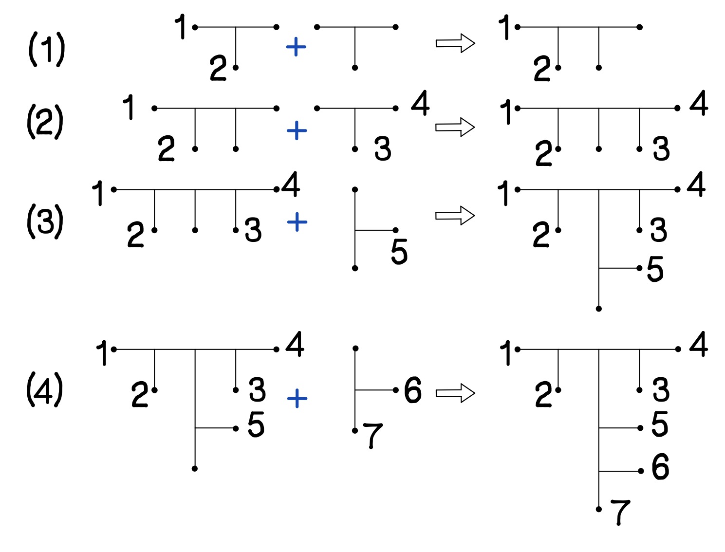
Any tree with more than three leaves can be formed by concatenating a three-leaf tree in the way described in Theorem 2.8 via iteration. See Figure 10 for an example. Using the last equation from Theorem 2.8, the number of edges in Connection Graph is
because
By solving the recurrence relation, we get the following explicit formula:
∎
3 Discussion
The purpose of this manuscript is to provide a combinatorial method to transition between copies of where is allowed to vary. Our combinatorial method only uses the intrinsic geodesic metric of (Owen and Provan, 2011) and the construction of the Connection Space, rather than introducing a complex system of mathematical objects that make our results applicable only in limited situations-meaning situations where there are limits on the number of taxa, types of data (meaning conspecific data, gene data, or species trees that should be combined), or the shape of the input and output trees. In particular, the types of tree topologies in the start tree in the beginning of the transition and the end of the the transition are not limited beyond the constraint that they are binary. We make these comments to emphasize that our combinatorial method opens the door to the study of several problems in computational biology that up to this point were impossible to study in spaces. We list a few examples below.
- 1.
There is potential for new supertree construction methods (that widely vary and are still under development) for combining phylogenies on varying numbers of taxa with myriad biological properties (Wilkinson et al., 2005; Bininda-Emonds, 2004; Akanni et al., 2015). Supertree methods must take inputs with varying numbers of taxa to be useful in a biological context. But in (St. John, 2017) it was made clear that spaces are well-suited for these methods due to the properties of the intrinsic geodesic metric.
- 2.
There is potential for new summary (coalesent-based) methods such as those developed in (Mirarab et al., 2014; Liu et al., 2015) that combine gene phylogenies such as in (Joyner et al., 2014) inferred from short samples from long genomes into a species phylogeny. In practice, it is rare that genomic information for all species taxa is available, and complex methods for dealing with this issue are of current interest to the computational biology community (Streicher et al., 2015; Darriba et al., 2016; Baca et al., 2017) when working with biological data. Summary methods are controversial (Chou et al., 2015; Springer and Gatesy, 2016), but remain of deep interest to the computational biology community and always require exceptions and non-trivial software advances for cases with missing taxa that appeal to complex solutions (Xi et al., 2015). While new methods for dealing with missing taxa are in constant production using computational techniques (Kobert et al., 2016; Thomas et al., 2013; Molloy and Warnow, 2017), it would be surprising if these results did not open the door to the use of spaces in novel quantitative paradigms for the development of fast and accurate novel methods for summary-based species tree estimation.
- 3.
Consensus methods such as the majority consensus method can achieve better results when there is not a restriction on the input trees having the same number of taxa. As pointed out in (St. John, 2017) the geodesic metric allows the construction of paths between trees in a set of trees in spaces that do not inherit splits from trees not in the set . Therefore our results may enable a novel quantitative embedding of the consensus problem for phylogenies that is competitive with our outperforms pre-existing methods. We believe this is a natural extension of this project because consensus methods rely on splits, but spaces have geometric components that allow for polytomic trees, which are not informative in the use of consensus methods that rely on resolved internal splits in a phylogeny.
- 4.
There is also potential for optimization of the results in this paper by further study of the Connection Space and the Connection Cluster. These are novel objects that may provide a more accessible quantitative framework for addressing problems such as quartet-agglomeration (Sumner et al., 2017; Sayyari and Mirarab, 2016; Reaz et al., 2014; Avni et al., 2015; Rusinko and Hipp, 2012) that require combining four-taxon trees into trees with any possible number of taxa. We mention the example of quartet-agglomeration in particular because, as explained thoroughly in (Sumner et al., 2017), the Neighbor-Joining method of tree inference (Saitou and Nei, 1987) is fundamentally a quartet-based method that continues to perform well on many datasets that contain more than four taxa (Yoshida and Nei, 2016). The scientific connection between quartet-agglomeration and Neighbor-Joining should not be ignored if progress in these areas is to be made, and our results provide a way to study these problems in a new setting.
- 5.
Finally, there is potential for using our new quantitative framework in the study of inferred unrooted trees that contain polytomies (vertices of degree of four or higher). The orthants of non-maximal dimension in any -space correspond to polytomic trees. Polytomies are often recovered in studies of biological data due to the fact that the biological signal in any dataset may not be strong enough to indicate that branch length in an inferred tree should have length greater than zero. This is known to be an issue in maximum-likelihood tree estimation on biological datasets (Pamminger and Hughes, 2017; Simmons and Norton, 2014; Slowinski, 2001). Further, it is known that if the true evolutionary history cannot provide sufficient information to resolve a polytomy, distance-based methods, which remain in use not only on their own, but also as components of maximum-likelihood phylogenomic software inference packages such as FastTree-2 (Price et al., 2010) are biased against returning the correct tree (Davidson and Sullivant, 2014).
4 Supporting materials
To generate connection graphs connecting spaces of specific dimensions using our software, use the script connection graph.py which includes dependencies on Dendropy (see (Sukumaran and Holder, 2010) for the original paper about this software package). Go to
https://github.com/cpmoni/igl-polyhedra
to find installation and usage instructions. Figure 11 is the connection graph generated to connect spaces between 9 and 10 dimensions. Please note that the other graphs in this paper is drawn by hand rather than the software, in order to fully clarify the mathematical concepts.

generated by the code released on the github with this paper
5 Acknowledgments
The undergraduate students Y.R, S.Z, J.B., and J. S., as well as the initialization of this project, were supported by a Mathways Grant NSF DMS-1449269 to the Illinois Geometry Lab at the University of Illinois Urbana-Champaign. R.D. was supported by the NSF grant DMS-1401591. M.D. was supported by the NSF Graduate Research Fellowship DGE-1144245. C.M. was supported by a GAANN fellowship from the Department of Education awarded by the University of Illinois Urbana-Champaign.
References
- Billera et al. (2001) L. J. Billera, S. P. Holmes, and K. Vogtmann, “Geometry of the space of phylogenetic trees”, Advances in Applied Mathematics 27 (2001), no. 4, 733–767.
- Owen and Provan (2011) M. Owen and J. S. Provan, “A fast algorithm for computing geodesic distances in tree space”, IEEE/ACM Transactions on Computational Biology and Bioinformatics (TCBB) 8 (2011), no. 1, 2–13.
- Benner et al. (2014) P. Benner, M. Bačák, and P.-Y. Bourguignon, “Point estimates in phylogenetic reconstructions”, Bioinformatics 30 (2014), no. 17, i534–i540.
- Nye (2011) T. M. Nye, “Principal components analysis in the space of phylogenetic trees”, The Annals of Statistics, 2011 2716–2739.
- Barden et al. (2013) D. Barden, H. Le, M. Owen, et al., “Central limit theorems for Fréchet means in the space of phylogenetic trees”, Electronic Journal of Probability 18 (2013).
- Miller et al. (2015) E. Miller, M. Owen, and J. S. Provan, “Polyhedral computational geometry for averaging metric phylogenetic trees”, Advances in Applied Mathematics 68 (2015) 51–91.
- Weyenberg et al. (2016) G. Weyenberg, R. Yoshida, and D. Howe, “Normalizing kernels in the Billera-Holmes-Vogtmann treespace”, IEEE/ACM Transactions on Computational Biology and Bioinformatics (TCBB), 2016.
- Lin et al. (2015) B. Lin, B. Sturmfels, X. Tang, and R. Yoshida, “Convexity in tree spaces”, arXiv preprint arXiv:1510.08797, 2015.
- Skwerer et al. (2014) S. Skwerer, J. Marron, and S. Provan, “Optimization methods for Fréchet means in BHV treespace”, arXiv preprint arXiv:1411.2923, 2014.
- Kim et al. (2016) S. Kim, C.-S. Cho, K. Han, and J. Lee, “Structural variation of Alu element and human disease”, Genomics and Informatics 14 (2016), no. 3, 70–77.
- Francis (2014) A. R. Francis, “An algebraic view of bacterial genome evolution”, Journal of Mathematical Biology 69 (2014), no. 6-7, 1693–1718.
- Abby et al. (2012) S. S. Abby, E. Tannier, M. Gouy, and V. Daubin, “Lateral gene transfer as a support for the tree of life”, Proceedings of the National Academy of Sciences 109 (2012), no. 13, 4962–4967.
- Joyner et al. (2014) J. Joyner, D. Wanless, C. D. Sinigalliano, and E. K. Lipp, “Use of quantitative real-time PCR for direct detection of serratia marcescens in marine and other aquatic environments”, Applied and Environmental Microbiology 80 (2014), no. 5, 1679–1683.
- Semple and Steel (2003) C. Semple and M. A. Steel, “Phylogenetics”, Oxford University Press on Demand, 2003.
- Lin and Yoshida (2016) B. Lin and R. Yoshida, “Tropical Fermat-Weber points”, arXiv preprint arXiv:1604.04674, 2016.
- Wilkinson et al. (2005) M. Wilkinson, J. A. Cotton, C. Creevey, O. Eulenstein, S. R. Harris, F.-J. Lapointe, C. Levasseur, J. O. Mcinerney, D. Pisani, and J. L. Thorley, “The shape of supertrees to come: tree shape related properties of fourteen supertree methods”, Systematic Biology 54 (2005), no. 3, 419–431.
- Bininda-Emonds (2004) O. R. Bininda-Emonds, “Phylogenetic supertrees: combining information to reveal the tree of life”, Springer Science & Business Media, 2004.
- Akanni et al. (2015) W. A. Akanni, M. Wilkinson, C. J. Creevey, P. G. Foster, and D. Pisani, “Implementing and testing bayesian and maximum-likelihood supertree methods in phylogenetics”, Royal Society Open Science 2 (2015), no. 8, 140436.
- St. John (2017) K. St. John, “The shape of phylogenetic treespace”, Systematic Biology 66 (2017), no. 1, e83–e94.
- Mirarab et al. (2014) S. Mirarab, R. Reaz, M. S. Bayzid, T. Zimmermann, M. S. Swenson, and T. Warnow, “ASTRAL: genome-scale coalescent-based species tree estimation”, Bioinformatics 30 (2014), no. 17, i541–i548.
- Liu et al. (2015) L. Liu, S. Wu, and L. Yu, “Coalescent methods for estimating species trees from phylogenomic data”, Journal of systematics and evolution 53 (2015), no. 5, 380–390.
- Streicher et al. (2015) J. W. Streicher, J. A. Schulte, and J. J. Wiens, “How should genes and taxa be sampled for phylogenomic analyses with missing data? an empirical study in iguanian lizards”, Systematic Biology 65 (2015), no. 1, 128–145.
- Darriba et al. (2016) D. Darriba, M. Weiß, and A. Stamatakis, “Prediction of missing sequences and branch lengths in phylogenomic data”, Bioinformatics 32 (2016), no. 9, 1331–1337.
- Baca et al. (2017) S. M. Baca, A. Alexander, G. T. Gustafson, and A. E. Z. Short, “Ultraconserved elements show utility in phylogenetic inference of Adephaga (Coleoptera) and suggest paraphyly of ‘Hydradephega”’, Systematic Entomology, 2017.
- Chou et al. (2015) J. Chou, A. Gupta, S. Yaduvanshi, R. Davidson, M. Nute, S. Mirarab, and T. Warnow, “A comparative study of SVDquartets and other coalescent-based species tree estimation methods”, BMC Genomics 16 (2015), no. 10, S2.
- Springer and Gatesy (2016) M. S. Springer and J. Gatesy, “The gene tree delusion”, Molecular phylogenetics and evolution 94 (2016) 1–33.
- Xi et al. (2015) Z. Xi, L. Liu, and C. C. Davis, “The impact of missing data on species tree estimation”, Molecular Biology and Evolution 33 (2015), no. 3, 838–860.
- Kobert et al. (2016) K. Kobert, L. Salichos, A. Rokas, and A. Stamatakis, “Computing the internode certainty and related measures from partial gene trees”, Molecular Biology and Evolution 33 (2016), no. 6, 1606–1617.
- Thomas et al. (2013) G. H. Thomas, K. Hartmann, W. Jetz, J. B. Joy, A. Mimoto, and A. O. Mooers, “PASTIS: an R package to facilitate phylogenetic assembly with soft taxonomic inferences”, Methods in Ecology and Evolution 4 (2013), no. 11, 1011–1017.
- Molloy and Warnow (2017) E. Molloy and T. Warnow, “To include or not to include: The impact of gene filtering on species tree estimation methods”, Systematic Biology, 2017 https://doi.org/10.1093/sysbio/syx077.
- Sumner et al. (2017) J. G. Sumner, A. Taylor, B. R. Holland, and P. D. Jarvis, “Developing a statistically powerful measure for quartet tree inference using phylogenetic identities and Markov invariants”, Journal of Mathematical Biology, 2017 1–36.
- Sayyari and Mirarab (2016) E. Sayyari and S. Mirarab, “Anchoring quartet-based phylogenetic distances and applications to species tree reconstruction”, BMC Genomics 17 (2016), no. 10, 783.
- Reaz et al. (2014) R. Reaz, M. S. Bayzid, and M. S. Rahman, “Accurate phylogenetic tree reconstruction from quartets: A heuristic approach”, PLoS One 9 (2014), no. 8, e104008.
- Avni et al. (2015) E. Avni, R. Cohen, and S. Snir, “Weighted quartets phylogenetics”, Systematic Biology 64 (2015), no. 2, 233–242.
- Rusinko and Hipp (2012) J. P. Rusinko and B. Hipp, “Invariant based quartet puzzling”, Algorithms for Molecular Biology 7 (2012), no. 1, 35.
- Saitou and Nei (1987) N. Saitou and M. Nei, “The neighbor-joining method: a new method for reconstructing phylogenetic trees.”, Molecular Biology and Evolution 4 (1987), no. 4, 406–425.
- Yoshida and Nei (2016) R. Yoshida and M. Nei, “Efficiencies of the NJp, maximum likelihood, and Bayesian methods of phylogenetic construction for compositional and noncompositional genes”, Molecular Biology and Evolution 33 (2016), no. 6, 1618–1624.
- Pamminger and Hughes (2017) T. Pamminger and W. O. H. Hughes, “Testing the reproductive groundplan hypothesis in ants (Hymenoptera: Formicidae)”, Evolution 71 (2017), no. 1, 153–159.
- Simmons and Norton (2014) M. P. Simmons and A. P. Norton, “Divergent maximum-likelihood-branch-support values for polytomies”, Molecular Phylogenetics and Evolution 73 (2014) 87–96.
- Slowinski (2001) J. B. Slowinski, “Molecular polytomies”, Molecular Phylogenetics and Evolution 19 (2001), no. 1, 114–120.
- Price et al. (2010) M. N. Price, P. S. Dehal, and A. P. Arkin, “FastTree 2–approximately maximum-likelihood trees for large alignments”, PloS one 5 (2010), no. 3, e9490.
- Davidson and Sullivant (2014) R. Davidson and S. Sullivant, “Distance-based phylogenetic methods around a polytomy”, IEEE/ACM Transactions on Computational Biology and Bioinformatics (TCBB) 11 (2014), no. 2, 325–335.
- Sukumaran and Holder (2010) J. Sukumaran and M. T. Holder, “Dendropy: a python library for phylogenetic computing”, Bioinformatics 26 (2010), no. 12, 1569–1571.