Suppressing epidemic spreading in multiplex networks with social-support

To investigate how degree heterogeneity affects spreading dynamics, we disallow any edge overlap between the two layers, i.e., nodes are randomly connected by edges in layer $S$ and layer $C$, and the amount of edge overlap $m_{e}$ is approximately 0 in the thermodynamic limit.

To examine $\rho$ as a function of $\beta$, we randomly select one percent of the nodes to be seeds ($\rho(0)=0.01$). Figure 2(a) shows the epidemic spreading for $\gamma=2.4$ and $\gamma=3.2$. Note the hybrid phase transition in $\rho$ that exhibits properties of both continuous and discontinuous phase transitions. As $\beta$ increases $\rho$ grows continuously at $\beta_{\rm inv}^{I}$. Then an infinitely small increase in $\beta$ induces an sudden jump of $\rho$ at $\beta_{\rm inv}^{II}$, where $\beta_{\rm inv}^{I}$ and $\beta_{\rm inv}^{II}$ are the first and second invasion thresholds. The $\rho$ transition type indicates that there are three possible system states, (i) completely healthy, (ii) partially infected, and (iii) completely infected. This differs significantly from the classical SIS model. In addition, we find hysteresis loops in the phase transition of $\rho$ when $\gamma=2.4$ and $\gamma=3.2$ [see Fig. 2(a)]. When the seed density is initially low, e.g., $\rho(0)=0.01$, the disease breaks out at the invasion threshold $\beta_{\rm inv}^{I}$, but when it is initially high, e.g., $\rho(0)=0.9$, the disease breaks out at the persistence threshold $\beta_{\rm per}$. The arrows in Fig. 2(a) indicate the direction of the hysteresis loops. We determine critical points $\beta_{\rm inv}^{I}$ and $\beta_{\rm inv}^{II}$ and persistence threshold $\beta_{\rm per}$ using the susceptibility $\chi$ shown in Fig. 2(b). The theoretical results obtained from the numerical iterations agree with the simulation results [see the lines in Fig. 2(a)].

We next determine how degree heterogeneity (i.e., parameter $\gamma$) influences the spreading dynamics. Figure 3(a) shows the two-parameter $(\beta,\gamma)$ phase diagram. The parameter space is partitioned into three regions according to $\rho$ value. When $\beta<\beta_{\rm inv}^{I}$, the system falls into the no-epidemic regime, i.e.,the green and part of the purple area below $\beta_{\rm inv}^{I}$. When $\beta_{\rm inv}^{I}\leq\beta<\beta_{\rm inv}^{II}$, it falls into the low-epidemic regime (bounded by two critical lines) in which $\rho$ increases slowly with $\beta$. Finally, above $\beta_{\rm inv}^{II}$, $\rho$ suddenly jumps to the high epidemic regime (red) in which approximately all nodes are infected. The regime between invasion threshold $\beta_{\rm inv}^{II}$ and persistence threshold $\beta_{\rm per}$ is the hysteresis region (purple). The values of $\beta_{\rm inv}^{I}$ and $\beta_{\rm inv}^{II}$ both increase with $\gamma$. Although we can obtain the theoretical value of $\beta_{\rm inv}^{I}$ from Eq. (16), we cannot obtain the theoretical value of $\beta_{\rm inv}^{II}$ and $\beta_{\rm per}$ by linearizing the equations around $\rho_{i}\rightarrow 0$ and $\theta_{j\rightarrow i}\rightarrow 0$ and thus we must apply numerical methods using Eqs. (4) and (6). We first define a judgment value $\epsilon$ that is linear with system size $N$. Without loss of generality we set $\epsilon=0.3$. We then define the jump size $\Delta\rho$ to be

where $\Delta\beta$ is an infinitesimal increment in $\beta$, which we set at $\Delta\beta=0.001$, and $\rho(\beta)$ is the infected density in the steady state when the transmission rate is $\beta$. We obtain the threshold when $\Delta\rho\geq\epsilon$ is at a certain $\beta$ value in the thermodynamic limit [47, 16]. Using the numerical method, we obtain the second invasion threshold $\beta_{\rm inv}^{II}$ and the persistence threshold $\beta_{\rm per}$. Figure 3 shows that the theoretical values marked by dotted lines agree with the simulation results. The change in the system state among the three regions indicates that the phase transitions of $\rho$ are hybrid. Figure 3(a) shows that the low epidemic and hysteresis regions expand as $\gamma$ increases.

To demonstrate that there are two invasion thresholds in networks with heterogeneous degree distribution, we use a finite-size scaling analysis [48]. Figure 3(b) shows the interval in $\beta_{\rm inv}^{I}\leq\beta<\beta_{\rm inv}^{II}$, which we denote $\|\beta_{\rm inv}^{II}-\beta_{\rm inv}^{I}\|$, as a function of $N$ for $\gamma=2.0$, $\gamma=2.2$, and $\gamma=2.8$, where $\|\bullet\|$ is the norm operator. Figure 3(b) shows the values of $\|\beta_{\rm inv}^{II}-\beta_{\rm inv}^{I}\|$ converging asymptotically to positive constant values in the thermodynamic limit, i.e., ${\lim_{N\to\infty}\|\beta_{\rm inv}^{II}-\beta_{\rm inv}^{I}\|}\simeq 0.006$ for $\gamma=2.0$, ${\lim_{N\to\infty}\|\beta_{\rm inv}^{II}-\beta_{\rm inv}^{I}\|}\simeq 0.008$ for $\gamma=2.2$, and ${\lim_{N\to\infty}\|\beta_{\rm inv}^{II}-\beta_{\rm inv}^{I}\|}\simeq 0.026$ for $\gamma=2.8$, which implies the two invasion thresholds do not merge when $\gamma\leq 2.2$ and the two are always present in networks with a heterogeneous degree distribution.

To analyze the sudden jump of $\rho$ and the hysteresis loops, we examine the transmission process analytically using mean-field approximation in random regular networks (RRNs), which corresponds to the limit $\gamma\rightarrow\infty$. Through a bifurcation analysis we account for the existence of the sudden jump of $\rho$ and the hysteresis loops (see appendix information). Note that the first threshold $\beta_{\rm inv}^{I}$ disappears in the RRNs and the transition of $\rho$ is discontinuous when it is not hybrid [see Fig. 9(a)].

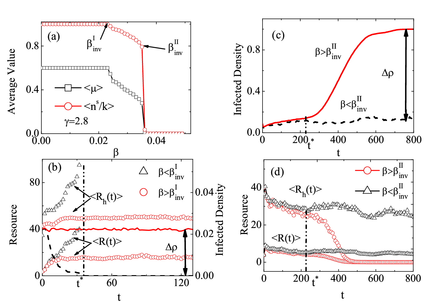
To explain the hybrid transition when $\gamma$ is finite, i.e., when $\gamma\leq 3.2$, we investigate the number of susceptible neighbors around each infected node in layer $S$ and their recovery rates as a function of $\beta$. In the steady state the number of each infected node’s susceptible neighbors in layer $S$ is $n_{s_{i}}$ and their fraction $n_{s_{i}}/k_{i}$. Here the recovery rate is $\mu_{i}$. To evaluate the collective state, we examine the average quantity $\langle n_{s}/k\rangle$ of $n_{s_{i}}/k_{i}$ and the average quantity $\langle\mu\rangle$ of the recovery rate. Figure 4(a) shows plots of $\langle n_{s}/k\rangle$ and $\langle\mu\rangle$ as functions of $\beta$ for $\gamma=2.8$. We find that both $\langle n_{s}/k\rangle$ and $\langle\mu\rangle$ are constant when $\beta<\beta_{\rm inv}^{I}$, which implies zero values for $\rho$. They then slowly decrease until they reach the $\beta_{\rm inv}^{II}$, at which point an infinitesimal increase in $\beta$ causes a jump in $\langle n_{s}/k\rangle$ and $\langle\mu\rangle$. Figures 4(b)–4(d) show the time dependence near $\beta_{\rm inv}^{I}$ and $\beta_{\rm inv}^{II}$. Figure 4(b) shows the time evolution of the infected density $\rho(t)$ around $\beta_{\rm inv}^{I}\simeq 0.023$ for $\gamma=2.8$. The difference in $\rho(\infty)$ for $\beta$ just below and above threshold $\beta_{\rm inv}^{I}$ is $\Delta\rho$ [see Eq. (18)]. Note that $\rho(\infty)$ increases slowly at $\beta_{\rm inv}^{I}$, i.e., a small increment $\Delta\rho\simeq 0.022$. We next examine the time evolutions of the average resources of the infected nodes $\langle R(t)\rangle$ and the hub nodes $\langle R_{h}(t)\rangle$. Note that without loss of generality we can assign hub node status to nodes with a degree larger than $k=30$. Note also that when $\beta$ is just below $\beta_{\rm inv}^{I}$ both $\langle R(t)\rangle$ and $\langle R_{h}(t)\rangle$ increase until $t=t^{*}$, which implies that all infected nodes have acquired sufficient resources to recover and $\rho(t)$ drops to zero. In contrast, when $\beta$ is just above $\beta_{\rm inv}^{I}$ and the transmission rate is low, the promotion effect of the hub nodes allows the disease to spread on a finite scale and infected nodes have sufficient resources for recovery. Thus infection and recovery processes are balanced, and the values of $\langle R(t)\rangle$ and $\langle R_{h}(t)\rangle$ fluctuate around a finite value when $t\rightarrow t_{\infty}$ [see Fig. 4(b)]. As $\beta$ smoothly increases at $\beta=\beta_{\rm inv}^{I}$, the level of available resources decreases continuously as the number of infected nodes increases [see Figs. 4(a)]. Thus the density of infection increases continuously at $\beta_{\rm inv}^{I}$. Figures 4(c) and 4(d) show a critical time $t^{*}\simeq 220$ at which $\beta$ is approximately $\beta_{\rm inv}^{II}\simeq 0.033$. At the early stage of the propagation process, i.e., when $t<t^{*}$, the disease spreads through the local seed nodes. Because most of neighbors of the infected nodes in layer $S$ remain healthy, they have a sufficient resource level to recover. Here the infection and recovery processes are balanced. As the $\rho(t)$ value increases slowly the available resources levels $\langle R_{h}(t)\rangle$ and $\langle R(t)\rangle$ for $\beta\simeq\beta^{II}_{\rm inv}$ slowly decrease [see Figs. 4(c) and 4(d)]. When $\beta<\beta^{II}_{\rm inv}$ the infection and recovery processes remain balanced when $t\rightarrow\infty$, thus the density of infection fluctuates around a small finite value when $t\rightarrow t_{\infty}$ ($\rho(\infty)\simeq 0.18$) [see Fig. 4(c)]. Because infection and recovery processes are balanced in $\beta^{I}_{\rm inv}\leq\beta<\beta^{II}_{\rm inv}$, the value of $\rho$ increases slowly. Note that as hub nodes disappear in the RRNs the disease is suppressed until $\beta$ reaches a threshold at which point it jumps discontinuously, the balance disappears (see Appendix), and only one threshold remains. When $\beta>\beta^{II}_{\rm inv}$ the transmission rate is relatively large and the balance between infection and recovery is broken. Infecting the healthy nodes in layer $C$ decreases the resources available to the nodes in layer $S$ and delays the recovery of infected nodes. This recovery delay increases the effective transmission probability in layer $C$, more healthy nodes are infected, and both the available resources and the recovery rate decrease. This causes a cascading infection in system nodes that is accelerated when hub nodes are surrounded by infected nodes, and this can cause total system failure. Figure 4(d) shows an abrupt drop of $\langle R_{h}(t)\rangle$ and $\langle R(t)\rangle$ at $t^{*}$ when $\beta>\beta^{II}_{\rm inv}$. Figure 4(c) shows a rapid increase in the density of infection from a small value $\rho(t^{*})\simeq 0.18$ to a high value $\rho(\infty)\simeq 1.0$. Note that in the steady state the large difference $\Delta\rho$ between $\beta<\beta_{\rm inv}^{II}$ and $\beta>\beta_{\rm inv}^{II}$ causes explosive transitions. This explains the hybrid transition in networks with a heterogeneous degree distribution.

Figure 4(d) shows the evolution of the resource level in the hub nodes. This explains the decrease in the two invasion thresholds and the gap that appears between the two thresholds with the increase of degree heterogeneity. A more heterogeneous network has more hub nodes and is more sensitive to increases in $\beta$. Thus increasing the degree heterogeneity reduces the gap between the two thresholds [see Fig. 3].

These numerical and simulation results differ greatly from the classical SIS model. In the multiplex networks with a heterogeneous degree distribution, degree heterogeneity enhances disease spreading and the phase transition is hybrid. Besides, there are hysteresis loops in the phase transition of $\rho$, and the interval between the two invasion thresholds and the hysteresis region decreases as degree heterogeneity increases. When $\gamma\rightarrow\infty$ the network is approximately a RRN, $\beta_{\rm inv}^{I}$ disappears as hub nodes disappear, and the transition is discontinuous.

In social networks two individuals can be friends in the social relation layer and coworkers in the physical contact layer. In transportation networks two cities can be connected by both an expressway and a railway. Thus edge overlap is essential in the science of complex networks, especially when studying percolation in multiplex networks [49]. Here we examine how the amount of edge overlap $m_{e}$ between the two layers affects the spreading dynamics. To eliminate the effect of structure, we fix the values $\gamma=2.2$ and $<k>=9$. We then use UCM to build a multiplex network with two identical layers $m_{e}=1.0$. To generate a variety of $m_{e}$ values, with a probability $q=1-m_{e}$ we rewire pairs of links in layer $S$.

Figure 5(a) shows a plot of $\rho$ as a function of $\beta$ with two typical values $m_{e}=1.0$ and $m_{e}=0.2$. Note that when the edges between the two layers overlap completely ($m_{e}=1.0$) the infected density $\rho$ smoothly increases from 0 to 1 and there is no hysteresis loop. When the rate of edge overlap between two layers is lowered, i.e., when $m_{e}=0.2$, a hybrid phase transition appears. The infected density $\rho$ smoothly increases at $\beta=\beta_{\rm inv}^{I}$ and then the system acquires a low epidemic region ($\beta_{\rm inv}^{I}<\beta<\beta_{\rm inv}^{II}$) in which $\rho$ slowly increases. Subsequently at $\beta=\beta_{\rm inv}^{II}$ an infinitesimally small increase in $\beta$ causes an abrupt jump in $\rho$ and the disease suddenly spreads throughout the entire system. Hysteresis loops appear in the transition process and the arrows indicate their direction. Figure 5(b) shows that the invasion thresholds (i.e., $\beta_{\rm inv}^{I}$) and $\beta_{\rm inv}^{II}$ and the persistence threshold $\beta_{\rm per}$ are determined by the susceptibility $\chi$. Note that the hysteresis loop disappears when $m_{e}=1.0$, and it no longer satisfies the definition of $\epsilon>0.3$ at $\beta_{L}$. Thus $\beta_{L}$ is an inflection point at which the increase in $\rho$ accelerates. The theoretical results from the DMP method agree with the simulation results.

To determine how the amount of edge overlap between the two layers affects the spreading dynamics, we perform simulations for values of $m_{e}$ from 0 to 1 and obtain the space in the plane $(\beta,m_{e})$ shown in Fig. 6. The parameter space is separated into phase regions I and II by a critical value of edge overlap $m_{e}^{c}\simeq 0.8$. When $m_{e}<m_{e}^{c}$ the system falls into phase I in which the phase transition of $\rho$ is hybrid and the space is again separated into three regions by two invasion thresholds $\beta_{\rm inv}^{I}$ (lower blue circles) and $\beta_{\rm inv}^{II}$ (upper blue circles). When $\beta<\beta_{\rm inv}^{I}$ the system has a no-epidemic region (green) in which all nodes are healthy and in a steady state. When $\beta_{\rm inv}^{I}\leq\beta<\beta_{\rm inv}^{II}$ the system has a low-epidemic region (orange) in which the infected density $\rho$ increases continuously from 0 to a finite value until it reaches the second invasion threshold $\beta_{\rm inv}^{II}$. Figure 3(b) shows a small low-epidemic region when $m_{e}\leq 0.2$ such that when $\gamma=2.2$ and $m_{e}=0.0$ the value of $\|\beta_{\rm inv}^{II}-\beta_{\rm inv}^{I}\|$ converges to a non-zero constant value when $N\rightarrow\infty$. When $\beta\geq\beta_{\rm inv}^{II}$ the system jumps abruptly to a high epidemic region (red) in which the disease spreads throughout the entire system. The hysteresis loops (purple) appear in phase I. In contrast, when $m_{e}\geq m_{e}^{c}$ the system falls into phase II in which the phase transition of $\rho$ is continuous. The value of $\rho$ smoothly increases from 0 to 1 and the hysteresis loops disappear. Figure 6 shows that when $\beta<\beta_{\rm inv}^{I}$ the value of $\beta_{\rm inv}^{I}$ decreases as the amount of edge overlap increases. Here edge overlap promotes disease spreading. When $\beta\geq\beta_{\rm inv}^{I}$ the value of $\beta_{\rm inv}^{II}$ increases as the amount of edge overlap increases. Here edge overlap suppresses disease spreading. We obtain the theoretical value of $\beta_{\rm inv}^{I}$ using Eq. (16) and $\beta_{\rm inv}^{II}$ and $\beta_{\rm per}$ using the method in Section IV.A. Figure 6 shows that the theoretical values marked by the dotted lines agree with simulation results.

To clarify these results, Figs. 7(a) and (b) show a plot of the average recovery rate $\langle\mu\rangle$ and the number of susceptible neighbors around each infected individual $\langle n_{s}/k\rangle$ as functions of $\beta$. Note that when the two layers overlap completely ($m_{e}=1.0$), $\langle n_{s}/k\rangle$ and $\langle\mu\rangle$ decrease at the first threshold $\beta_{\rm inv}^{I}$ to a certain value and then decrease continuously to zero, indicating that the infected density in the steady state increases continuously up to 1 as $\beta$ increases. In contrast, when $m_{e}=0.5$ there are two abrupt jumps of $\langle n_{s}/k\rangle$ and $\langle\mu\rangle$ at $\beta_{\rm inv}^{I}$ and $\beta_{\rm inv}^{II}$, respectively. Here $\langle\mu\rangle$ jumps sharply to zero at $\beta_{\rm inv}^{II}$ [see Fig. 7(b)] indicating an explosive jump in $\rho$.

Figures 7(c) and 7(d) show the time dependence of the infected density and the resource value. Figure 7(c) shows the average resource of all infected nodes $\langle R(t)\rangle$ and the average resource of hub nodes $\langle R_{h}(t)\rangle$ as a function of $t$ for $m_{e}=1.0$. Note that when $\beta$ is immediately below $\beta_{\rm inv}^{I}$ both $\langle R_{h}(t)\rangle$ and $\langle R(t)\rangle$ increase continuously until $t=t^{*}$. When $t>t^{*}$ there is no definition of resource because all infected nodes recover [see $\rho(t)$ for $\beta<\beta_{\rm inv}^{I}$ at $t=t^{*}$]. When $\beta\geq\beta_{\rm inv}^{I}$ the infection and recovery rates are balanced, and both $\langle R_{h}(t)\rangle$ and $\langle R(t)\rangle$ fluctuate around a finite value when $t\rightarrow t_{\infty}$. Thus all the infected nodes recover with a certain probability and $\rho(t)$ also fluctuates around a finite value when $t\rightarrow t_{\infty}$ [see $\rho(t)$ for $\beta>\beta_{\rm inv}^{I}$]. With an increase in $\beta$, resource availability decreases continuously as the number infected nodes increases until the disease spreads throughout the system and no available resources remain [see Figs. 7(a) and 7(c)]. This accounts for the continuous increase in $\rho$ when $m_{e}=1.0$.

Figure 7(d) shows the time evolution of the infected density and available resource level for $m_{e}=0.5$. Note that when $\beta$ is immediately below $\beta_{\rm inv}^{II}$ at the early stage the disease propagates within the local range of seed nodes, and there are sufficient healthy neighbors in layer $S$ to temporarily suppress the spread. This causes a brief increase in available resources at the beginning of the propagation process and a slight decline in the density of infection. Subsequently the disease rapidly spreads along the edges in layer $C$. When edges in layer $S$ link out ($m_{e}=0.5$), with a high probability that infected nodes in layer $S$ infect their neighbors, $\langle R_{h}(t)\rangle$ and $\langle R(t)\rangle$ rapidly decline, and $\rho(t)$ rapidly increases. Eventually infection and recovery become balanced, and $\rho(t)$, $\langle R_{h}(t)\rangle$, and $\langle R(t)\rangle$ converge to finite values. When $\beta>\beta_{\rm inv}^{II}$ there is also a temporary increase in both the available resources and the density of infection. However, when the propagation begins, unlike when $m_{e}=1.0$ [see Figs. 4(c) and 4(d)] there is no balanced period at the beginning of the process. The infection of the $S$-state nodes reduces the resource available to a large number of infected nodes in layer $S$ and delays their recovery. This recovery delay further increases the transmission probability in layer $C$. Thus $\langle R_{h}(t)\rangle$ and $\langle R(t)\rangle$) decline sharply to zero, the density of infection rapidly increases to 1, and cascading infection occurs.

An increase in the overlap between two layers indicates an increase in the local social circle of an individual. When an individual’s colleagues (those frequently in contact, defined as the contact layer) and friends (the social relations, defined as the social layer) are the same group of people, the links in these two layers largely overlap. When $\beta<\beta_{\rm inv}^{I}$, seed nodes initially transmit the disease only to immediate neighbors with whom they are in frequent contact. This high-value local effect causes infected nodes to have a higher probability of linking with other infected nodes in layer $S$ and lowers the level of resources available from neighbors. Thus the overlap between two layers increases network fragility against the invasion of the disease, and increases the probability of an epidemic breakout, and thus lowers the epidemic threshold $\beta_{\rm inv}^{I}$. In contrast, a lower value of overlap rate between the two layers indicates a more global social circle, neighbors of nodes in the social layer differ from neighbors in the contact layer. The infected nodes in the contact layer can acquire resources from healthy neighbors in the social layer. Thus the network is more robust against the invasion of the disease, and there is a relatively high epidemic threshold $\beta_{\rm inv}^{I}$. This is the reason $\beta_{\rm inv}^{I}$ decreases as $m_{e}$ increases, as shown in Fig. 6. When $\beta_{\rm inv}^{I}\leq\beta<\beta_{\rm inv}^{II}$, hub nodes promote disease transmission, the disease breaks out in a finite range, a sufficient number of healthy neighbors are present in layer $S$ to help infected nodes to recover, and infection and recovery remain balanced. Figure 7(d) shows that the value of resource availability fluctuates around a finite value when $t\rightarrow t_{\infty}$, and the density of infection converges continuously to a finite value ($\rho\simeq 0.28$). Thus in this region the global connections in a social layer have an advantage over the local connections [see Fig. 5(a)]. When $\beta\geq\beta_{\rm inv}^{II}$ the disease breaks out rapidly and globally, and the balance between infection and recovery is broken. When $m_{e}<m_{e}^{c}$ (a relatively low overlap rate), the connections in layer $S$ are more global. The infection of a small number of S-state nodes in layer $C$ influences the recovery of a large number of I-state nodes in layer $S$. Thus there is a delay in the recovery of infected nodes that further increases the transmission probability, promotes the disease spreading in layer $C$, and causes global cascading failure. This explains the increase in $\beta_{\rm inv}^{II}$ with $m_{e}$ and the explosive jump of $\rho$ [see Fig. 7 (c)] when $m_{e}<m_{e}^{c}$. In contrast, when $m_{e}>m_{e}^{c}$, the connections of layer $S$ is more localized, and the infection of nodes in layer $C$ delays the recovery of the infected nodes within only a small range in layer $S$. This small range in recovery delay does not globally increase the effective transmission probability. Thus as the effective transmission probability gradually increases the value of $\rho$ smoothly increases with $\beta$ [see Figs. 7(a) and 7(c)].

References

- [1] Meyers L A, Pourbohloul B, Newman M E, Skowronski D M and Brunham R C 2005 J. Theor. Biol. 232 71.
- [2] Yuen K, Chan P, Peiris M, Tsang D, Que T, Shortridge K, Cheung P, et al., 1998 The Lancet 351 467.
- [3] de Jong M D, Simmons C P, Thanh T T, et al., 2006 Nat. Med. 12 1203.
- [4] Team W E R 2014 N. Engl. J. Med. 2014 1481.
- [5] Gallup J L and Sachs J D 2001 AM J. Trop. Med. Hyg. 64 85.
- [6] Kirigia J M, Sambo L G, Yokouide A, Soumbey-Alley E, Muthuri L K and Kirigia D G 2009 BMC International Health and Human Rights 9 8.
- [7] Stinnett A A and Paltiel A D, 1996 Journal of Health Economics 15 641.
- [8] Wang L Y, Haddix A C, Teutsch S M and Caldwell B 1999 AM. J. Manag. Care 5 445.
- [9] Zaric G S and Brandeau M L 2002 Math. Med. Biol. 19 235.
- [10] Brandeau M L, 2005 in Operations Research and Health Care (Springer).
- [11] Brandeau M L, Zaric G S and Richter A 2003 Journal of Health Economics 22 575.
- [12] Böttcher L, Woolley-Meza O, Araújo N A, Herrmann H J and Helbing D 2015 Sci. Rep. 5 16571
- [13] Araújo N A and Herrmann H J 2010 Phys. Rev. Lett. 105 035701.
- [14] Nagler J, Tiessen T and Gutch H W 2012 Phys. Rev. X 2 031009.
- [15] DSouza R M and Nagler J 2015 Nat. Phys. 11 531.
- [16] Chen X L, Yang C, Zhong L F and Tang M 2016 Chaos 26 083114.
- [17] Boccaletti S, Almendral J, Guan S et. al. 2016 Phys. Rep. 660 1.
- [18] Chen X L, Zhou T, Feng L, Yang C, Wang M M, Fan X M and Hu Y Q, 2016 arXiv:1611.00212.
- [19] Böttcher L, Woolley-Meza O, Goles E, Helbing D and Herrmann H 2016 Phys. Rev. E 93 042315.
- [20] Seeman T E 1996 Ann. Epidemiol. 6 442.
- [21] Schulz R and Sherwood P R 2008 Journal of Social Work Education 44 105.
- [22] Drummond M F, Sculpher M J, Claxton K, Stoddart G L and Torrance G W 2015 Methods for the economic evaluation of health care programmes (Oxford university press).
- [23] Cohen S E and Syme S, 1985 Social support and health (Academic Press).
- [24] Thoits P A 1995 Journal of Health and Social Behavior 2 5379.
- [25] Gomez S, Diaz-Guilera A, Gomez-Gardenes J, Perez-Vicente C J, Moreno Y and Arenas A 2013 Phys. Rev. Lett. 110, 028701.
- [26] Granell C, Gomez S and Arenas A 2013 Phys. Rev. Lett. 111 128701.
- [27] Bianconi G and Radicchi F 2016 arXiv:1610.08708.
- [28] De Domenico M, Granell C, Porter M A and Arenas A 2016 Nat. Phys. 12 901906.
- [29] Karrer B and Newman M E 2010 Phys. Rev. E 82 016101.
- [30] Shrestha M and Moore C 2014 Phys. Rev. E 89 022805.
- [31] Shrestha M, Scarpino S V and Moore C 2015 Phys. Rev. E 92 022821.
- [32] Wang W, Tang M, Stanley H E and Braunstein L A 2017 Rep. Prog. Phys. 80 036603.
- [33] Guimera R, Mossa S, Turtschi A and Amaral L N 2005 Proc. Natl. Acad. Sci. USA 102 7794.
- [34] Bullmore E and Sporns O 2012 Nat. Rev. Neurosci.13 336.
- [35] Valdez L D, Di Muro M A and Braunstein L A 2016 J. Stat. Mech-Theory E 2016 093402.
- [36] Pastor-Satorras R and Vespignani A 2001 Phys. Rev. Lett. 86 3200.
- [37] Pastor-Satorras R, Castellano C, Van Mieghem P and Vespignani A 2015 Rev. Mod. Phys. 87 925.
- [38] Gomez S, Arenas A, Borge-Holthoefer J, Meloni S and Moreno Y 2010 Europhys. Lett. 89 38009.
- [39] Krzakala F, Moore C, Mossel E, Neeman J, Sly A, Zdeborova L and Zhang P 2013 Proc. Natl. Acad. Sci. USA 110 20935.
- [40] Viswanath B, Mislove A, Cha M and Gummadi K P 2009 Proceedings of the 2nd ACM workshop on Online social networks pp: 37-42.
- [41] Adamic L A and Huberman B A 2000 Science 287 2115.
- [42] Catanzaro M, Boguñá M and Pastor-Satorras R 2005 Phys. Rev. E 71, 027103.
- [43] Boguna M, Pastor-Satorras R and Vespignani A 2004 Euro. Phys. J. B 38 205.
- [44] Pastor-Satorras R and Vespignani A 2001 Phys. Rev. Lett. 86 3200.
- [45] Ferreira S C, Castellano C and Pastor-Satorras R 2012 Phys. Rev. E 86 041125.
- [46] Shu P, Wang W, Tang M, Zhao P and Zhang Y C 2016 Chaos 26 063108.
- [47] Nagler J, Levina A and Timme M 2011 Nat. Phys. 7, 265.
- [48] Newman M and Barkema G 1999 Monte Carlo Methods in Statistical Physics (Oxford University Press).
- [49] Cellai D, Lopez E, Zhou J, Gleeson J P and Bianconi G 2013 Phys. Rev. E 88 052811.
- [50] Strogatz S 1994 Nonlinear dynamics and chaos: With applications (Addison-Wesley, Reading, MA).