Angular Superdiffusion and Directional Memory in Two-Dimensional Electron Fluids

Electrons in two-dimensional (2D) materials can feature striking non-Fermi-liquid behaviors that are not found in ordinary solids. One celebrated example is Dirac electrons in graphene, where long-range electron-electron (ee) interactions invalidate the free-particle picture at charge neutrality[1, 2, 3, 4, 5]. Strongly-correlated quasirelativistic Dirac fluids can exhibit a range of interesting quantum-critical and hydrodynamic behaviors [6, 7, 8, 9, 10, 11].

Here we argue that 2D Fermi gases with generic two-body interactions, e.g. such as those realized in graphene doped away from neutrality, also feature non-Fermi-liquid behavior, however of an entirely different kind. Namely, we predict dynamics with strong directional memory mediated by slow angular diffusion of excitations over the Fermi surface. Occurring at the timescales much longer than the conventional Fermi-liquid excitation lifetimes $\tau_{*}\sim 1/T^{2}$, such abnormally long-lived excitations define what may be appropriate to call a “super-Fermi-liquid” regime.

Finite lifetimes of quasiparticles with characteristic temperature dependence $\tau_{*}\sim 1/T^{2}$ are an essential feature of Landau Fermi-liquids[28, 29]. In three-dimensional (3D) systems, the timescale $\tau_{*}$ marks the onset of the hydrodynamic regime in which system memory of the microscopic state is fully erased. The 2D systems, however, have long been suspected to feature a behavior at $t>\tau_{*}$ that is considerably more complex and interesting than in 3D[30, 31, 32]. The unique aspect of 2D Fermi gases is that generic momentum-conserving particle collisions at a thermally blurred 2D Fermi surface are blocked by fermion exclusion, resulting in nontrivial constraints for the angles between momenta of colliding particles. The collinear processes singled out by these constraints, in particular their limited ability to provide angular relaxation, define a new dynamical regime for two-dimensional Fermi systems[33, 34]. Understanding the nature and wide implications of this new “super-Fermi-liquid” behavior remains an outstanding challenge.

The goal of this work is to provide insight into some of these questions. As we will see, the dynamics at times $t>\tau_{*}$ represents a new transport regime which is distinct from conventional hydrodynamics. While many degrees of freedom relax at the “normal” time scales $t\sim\tau_{*}$, many other degrees of freedom remain unrelaxed and active at times $t\gg\tau_{*}$. Specifically, the dynamics is of a very different nature for the even-parity and odd-parity parts of momentum distribution, $f_{\pm}({\boldsymbol{p}})$, defined with respect to inversion ${\boldsymbol{p}}\to-{\boldsymbol{p}}$. Estimates show that the dynamical time scales for the odd-parity degrees of freedom are much longer than for the even-parity ones[34],

$$\tau_{\rm odd}\sim(T_{F}/T)^{2}\tau_{\rm even},\quad\tau_{\rm even}\sim\tau_{*}.$$

(1)

The new regime spans the wide range of time scales

$$\tau_{\rm even}\ll t\ll\tau_{\rm odd},$$

(2)

followed by a transition to the conventional hydrodynamic regime at the longest times, $t\sim\tau_{\rm odd}\gg\tau_{*}$. The hierarchy of time scales and the new regime are illustrated in Fig.1. This hierarchy also translates, through the relation $\ell\sim v_{F}t$, into a new hierarchy of spatial scales (see discussion in Sec.V).

We will see that the dynamics of the odd-parity degrees of freedom features directional memory effects with long characteristic times, defining an interesting “tomographic” behavior. The long timescales arise due to many repeated collisions with small angular stepsizes. We are therefore led to consider random walks on the Fermi surface arising due to small momentum changes in two-particle collisions. Processes of this type are routinely modeled as Fokker-Planck diffusion. The momentum-space Fokker-Planck picture is applicable to a wide variety of systems, ranging from collisions in plasmas and electron-phonon scattering in metals to radiation transport in cosmology[35, 36].

In our case, however, the random-walk dynamics on the Fermi surface comes with a twist that sets it apart from all previously known cases. We will show that this random walk is essentially non-Brownian, governed by special two-particle collisions, illustrated in Fig.2, that are simultaneously soft and head-on. This leads to highly correlated angular displacements that are near-equal and opposite in each scattering process, enforced by kinematic constraints and fermion exclusion acting together. Such lock-step angular correlations produce a peculiar long-time angular dynamics of superdiffusive type:

$$\partial_{t}\tilde{f}(\theta)=-D\partial_{\theta}^{4}\tilde{f}(\theta),\quad\tilde{f}(\theta)=\frac{f(\theta)-f(\theta+\pi)}{2},$$

(3)

with $\theta$ the azimuthal angle on the Fermi surface and $\tilde{f}(\theta)$ the odd-parity part of momentum distribution. The angular (super)diffusion coefficient $D$ will be found to scale with temperature as $D\sim T^{4}/T_{F}^{3}$. The $T^{4}$ scaling, as well as the form of (3), are valid for not-too-small and not-too-large angular displacements, $\delta\theta\ll\theta\ll 2\pi$, with the UV cutoff $\delta\theta\sim\sqrt{T/T_{F}}$ and up to log corrections (see below).

Anomalous diffusion, described by the square of Laplacian in (3), may seem to be at odds with the central limit theorem (CLT) that links random walks with diffusive transport in suitably defined configuration space[37]. The unique aspect of our problem, which invalidates this CLT-based intuition, has to do with nontrivial correlations of angular displacements in two-body collisions. The latter make the “center of mass” of the distribution in the angle variable conserved not just on average but individually in each collision process. This property suppresses the conventional one-particle diffusivity, generating instead the two-particle superdiffusive behavior.

The educated reader would notice that the picture described above seems to contradict the analysis of excitation lifetimes based on the Green’s function selfenergy calculations, which for 2D Fermi liquids predicts log-enahnced decay rates that scale with temperature as $\gamma\sim T^{2}\log(T_F/T)$[12, 13, 14, 15, 16, 17, 18]. The selfenergy approach is therefore totally unaware of the existence of the long-lived excitations. This is because the selfenergy is most sensitive to the fastest decay pathways. If, as is often the case, there is a single timescale that characterizes decay for all low-energy excitations, the selfenergy is a signature of that timescale. Yet, the single-timescale assumption is completely untrue in 2D, since the relatively slow angular diffusion creates a wide spectrum of lifetimes, (2). The selfenergy approach is therefore not well suited for such a situation.

The fact that slow angular dynamics pushes the onset of the conventional hydrodynamic behavior to very long times has wide implications for the ongoing quest for hydrodynamics in 2D electron fluids [19, 20, 21, 22, 23, 24, 25, 26, 27], in which the directional memory effects have so far been ignored. We will comment on possible experiments that can probe angular dynamics in Sec.V.

To set the stage for analyzing superdiffusive behavior, we recall that kinematic constraints and fermion exclusion restrict momenta of particles colliding on a thermally broadened Fermi surface as [30, 31, 32]

	$\displaystyle$	$\displaystyle\rm{\displaystyle(i)}\quad{\boldsymbol{p}}_{1}=-{\boldsymbol{p}}_{2},\quad{\boldsymbol{p}}_{1^{\prime}}=-{\boldsymbol{p}}_{2^{\prime}}$		(4)
		$\displaystyle\rm{\displaystyle(ii)}\quad{\boldsymbol{p}}_{1}={\boldsymbol{p}}_{1^{\prime}},\quad{\boldsymbol{p}}_{2}={\boldsymbol{p}}_{2^{\prime}}$

where $1$, $2$ and $1^{\prime}$, $2^{\prime}$ label ingoing and outgoing states, respectively. These relations, which are true at leading order in $T\ll T_{F}$, and up to permutations of particles $1$ and $2$, imply that the even-parity and odd-parity degrees of freedom relax in very different ways. Namely, the even-parity degrees of freedom relax in a “normal” manner, through transferring particle distribution between distant points in momentum space in a single collision event, at a characteristic timescale $\tau_{\rm even}\sim 1/T^{2}$. In contrast, the odd-parity degrees of freedom remain unrelaxed at these timescales.

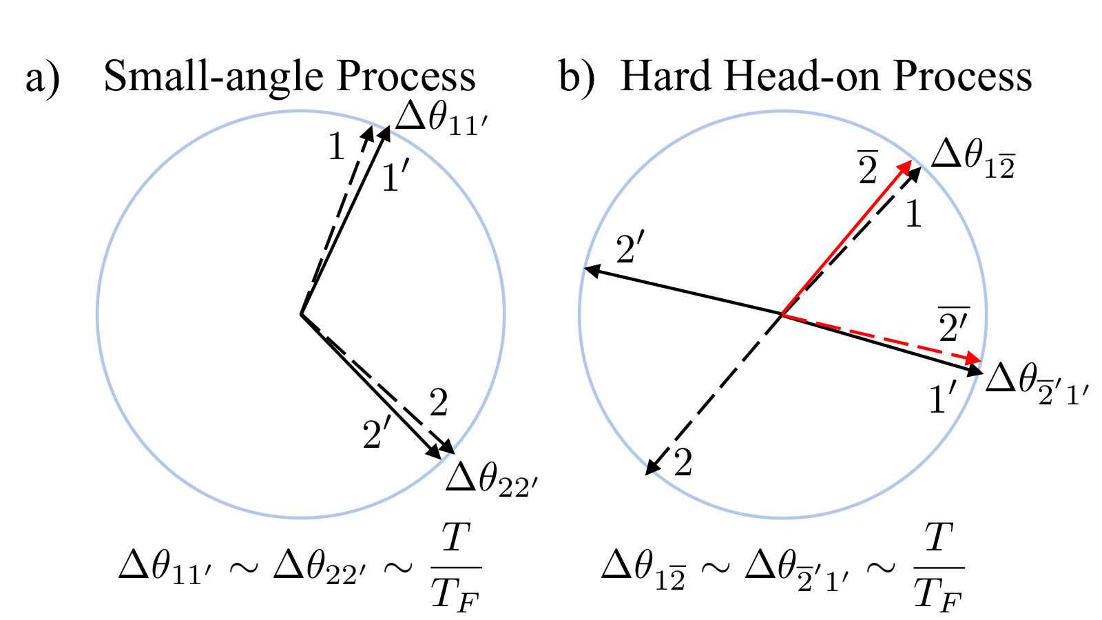
As we will see, the odd-parity degrees of freedom are frozen only at leading order in $T\ll T_{F}$. Letting momenta go slightly off the Fermi surface (by an amount proportional to temperature) unfreezes these degrees of freedom and generates a random walk in momentum space. The resulting angular dynamics is dominated by the soft head-on (SH) processes for which the two conditions in (4) are met simultaneously, such that all four momenta ${\boldsymbol{p}}_{1}$, ${\boldsymbol{p}}_{2}$, ${\boldsymbol{p}}_{1^{\prime}}$, ${\boldsymbol{p}}_{2^{\prime}}$ are near-collinear, as illustrated in Fig.2 b). As we will see, the SH processes define a non-Brownian random walk described as an anomalous diffusion with a square of Laplacian, (3) with $D\sim T^{4}/T_{F}^{3}$.

At the same time, the non-SH processes pictured in Fig.2 a) and c), taken alone, would lead to angular diffusion of a normal kind (see discussion in Sec.IV):

$$\frac{\partial}{\partial t}\delta f(\theta)=D^{\prime}\partial_{\theta}^{2}\delta f(\theta),\quad D^{\prime}\sim\frac{T^{4}}{T_{F}^{3}}.$$

(5)

Comparing to the dynamics in (3), we see that the diffusion in (5) is relatively more slow than that in (3) with the same diffusivity value, $D^{\prime}=D$. Indeed, in this case (3) predicts a faster spreading than (5) for not-too-long times:

$$\left\langle\delta\theta^{2}\right\rangle^{1/2}\approx(Dt)^{1/4}\gg(D^{\prime}t)^{1/2},\quad Dt\ll 1,$$

(6)

representing nothing but the inequality $x^{1/4}\gg x^{1/2}$, $x\ll 1$. (5) thus provides at most a subleading correction to (3).

We note parenthetically that terms fourth order in gradients usually arise in the theory of random walks as “subdiffusion” corrections to the diffusion equation. Indeed, gradient expansion in $\xi\partial_{\theta}$ with $\xi$ the random walker stepsize would yield terms $\left\langle\xi^{2}\right\rangle\partial_{\theta}^{2}$ and $\left\langle\xi^{4}\right\rangle\partial_{\theta}^{4}$ with the prefactors of the same order. Then, because $\xi$ is of a microscopic scale, one would have $D\ll D^{\prime}$. In our case, in contrast, for the SH processes the terms $\left\langle\xi^{2}\right\rangle\partial_{\theta}^{2}$ vanish because of the lock-step correlations (see discussion in Sec.IV), and the only remaining nonzero second-order contribution is the one of non-SH processes. The latter, however, have much smaller stepsizes than the SH processes, resulting in $D\sim D^{\prime}$. As a result, we have an interesting situation when the subdiffusion correction actually dominates. We will therefore use the name “superdiffusion” for (3).

The key difference between the SH and non-SH processes is in the size of angular displacements, which are order $\sqrt{T/T_{F}}$ for the SH processes and order $T/T_{F}$ for non-SH processes. These estimates can be obtained by expanding linearly in small deviations from the Fermi surface, such that particle energies are allowed to go off the Fermi level by an amount proportional to temperature. The analysis involves resolving kinematic constraints for scattering angles and specializing to small energy transfers $\omega$ limited by $T\ll T_{F}$. For simplicity, we assume a general isotropic carrier dispersion relation expanded in momentum deviations from the Fermi surface as

$$\varepsilon({\boldsymbol{p}})=\varepsilon_{F}+\frac{1}{2m_{*}}(p^{2}-p_{F}^{2}),$$

(7)

with the terms higher-order in the expansion parameter $\eta=p^{2}-p_{F}^{2}$ omitted for brevity. The resulting scattering angles $\theta_{1}$, $\theta_{1^{\prime}}$, $\theta_{2}$, $\theta_{2^{\prime}}$ dependence on momentum transfer ${\boldsymbol{q}}={\boldsymbol{p}}_{1^{\prime}}-{\boldsymbol{p}}_{1}={\boldsymbol{p}}_{2}-{\boldsymbol{p}}_{2^{\prime}}$ is obtained in Supplemental Information and is shown in Fig.2.

Angular relaxation is characterized by angular stepsizes $\Delta\theta$, which are marked in Fig.2. These quantities have a nonmonotonic dependence on $q$ such that the maximal stepsizes are reached for SH processes, when ${\boldsymbol{q}}$ is nearly perpendicular to ${\boldsymbol{p}}_{1}$, ${\boldsymbol{p}}_{1^{\prime}}$, ${\boldsymbol{p}}_{2}$, ${\boldsymbol{p}}_{2^{\prime}}$. In this case, the momentum transfer is estimated as

$$q\sim q_{T}=\sqrt{2m_{*}T}$$

(8)

with the energy transfer $\omega\sim T$ (see (S.1) and accompanying discussion). Because ${\boldsymbol{q}}$ is a vector that connects ${\boldsymbol{p}}_{1}$ and ${\boldsymbol{p}}_{1^{\prime}}$, we estimate the maximal angular displacement as

$$\Delta\theta=\frac{q}{p_{F}}\sim\sqrt{\frac{T}{T_{F}}}.$$

(9)

In contrast, for non-SH process the momenta ${\boldsymbol{p}}_{1}$, ${\boldsymbol{p}}_{1^{\prime}}$, ${\boldsymbol{p}}_{2}$, ${\boldsymbol{p}}_{2^{\prime}}$ are not nearly perpendicular to ${\boldsymbol{q}}$. In this case, $v_{F}q\sim\omega\sim T$ yields $\Delta\theta\sim T/T_{F}$. For larger values of $q$ the collision becomes hard head-on. As discussed in the next section and in the Supplemental Information, the relevant angular displacements in this case are $\Delta\theta_{1\bar{2}}=\theta_{1}-\theta_{\bar{2}}$ and $\Delta\theta_{\bar{2}^{\prime}1^{\prime}}=\theta_{\bar{2}^{\prime}}-\theta_{1^{\prime}}$ where $\theta_{\bar{2}}=\theta_{2}+\pi$ and $\theta_{\bar{2}^{\prime}}=\theta_{2^{\prime}}+\pi$. We will see that these stepsizes also scale as $T/T_{F}$ for hard head-on collisions, but scale as $\sqrt{T/T_{F}}$ for SH collisions (as shown in Fig.2).

This leads to two distinct types of angular steps: big ones for SH processes, and small ones for non-SH processes. Also, since $T\ll T_{F}$, typical $q$ values are quite small: $q/2k_{F}\sim\sqrt{T/T_{F}}\ll 1$. Accordingly, in Fig.2 we used (S.9) with $\omega=0.002T_{F}$.

The scaling $\Delta\theta\sim T$ and $\Delta\theta\sim\sqrt{T}$ for angular steps can also be inferred from a purely geometric argument. One can note an interesting property of the collisions which are depicted in Fig.5: the tips of four momentum vectors form rectangles. This rectangle property may be justified either by carrying out the above analysis further or, instead, by noting that the kinematics close to the Fermi level approximately follows a parabolic dispersion, (7). We may therefore boost to the center of mass frame, wherein the collisions become perfectly head-on. The scaling $T$ and $\sqrt{T}$ for angular steps then follows from inspecting the types of chords (momentum transfers) that can be drawn in an annulus of width $T$.

At this point, the reader may wonder whether the fine-tuned angles between momenta in SH collisions, which make the phase space for these processes small, will also reduce the SH collision rate. A detailed analysis shows that this is not the case[34]: instead, the two momentum delta functions are near-perfectly aligned and thus oversatisfied. This produces a well-known log enhancement of the collision rate, behaving as $\log(T_F/T)T^{2}/T_{F}$. For simplicity, this log enhancement will be ignored in subsequent analysis.

Here we will introduce a Fermi half-circle configuration space, in which the dynamics of the odd-parity distributions

$$\delta f(\theta)=-\delta f(\theta+\pi).$$

(10)

can be understood most clearly. The construction of half-circle configuration space is depicted in Fig.3b. First, angles $\theta$ and $\theta+\pi$ are “glued together” to form a circle of a two times smaller radius:

$$S^{1}/\mathbb{Z}_{2}=\mathbb{R}\rm{P}^{1}\simeq S^{1}.$$

(11)

In addition, anti-periodic boundary conditions are imposed on distribution functions, enforcing the odd-parity condition (10).

To describe the change of odd-parity distributions under collisions it is convenient to combine the odd-parity condition, (10), with symmetry between the ingoing and outgoing states, and introduce what we will refer to as “reflection” transformation. Indeed, for odd-parity distribution functions, adding a particle at $\theta$ is equivalent to removing a particle at $\theta+\pi$. Thus, ingoing (outgoing) momenta at angle $\theta$ should be identified with outgoing (ingoing) momenta at angle $\theta+\pi$, respectively. This is depicted in Fig.3a, with the ingoing and outgoing states $2$ and $2^{\prime}$ and the corresponding reflected outgoing and ingoing states $\bar{2}$ and $\bar{2}^{\prime}$ (red arrows).

Applying this transformation to an SH collision pictured in Fig.3b, we reflect one of the ingoing states, $2$, and one of the outgoing states, $2^{\prime}$, to obtain the outgoing state $\bar{2}$ and the ingoing state $\bar{2}^{\prime}$. We may then view the processes as a two-particle hopping on a half-circle: $1\to\bar{2}$ and $\bar{2}^{\prime}\to 1^{\prime}$, such that all states are positioned on the same small patch of the half-circle. The angular displacements after reflection, shown by arrows in Fig.3a, are then equal and opposite,

$$\Delta\theta_{1\bar{2}}=\theta_{1}-\theta_{\bar{2}},\quad\Delta\theta_{\bar{2}^{\prime},1^{\prime}}=\theta_{\bar{2}^{\prime}}-\theta_{1^{\prime}},$$

(12)

scaling with temperature as

$$\Delta\theta_{1\bar{2}}=-\Delta\theta_{\bar{2}^{\prime}1^{\prime}}\sim\sqrt{\frac{T}{T_{F}}}.$$

(13)

This defines a random walk process by which the odd-parity distribution changes, which we will use below to analyze superdiffusion.

The non-SH processes, which give a subleading contribution to angular dynamics, can be represented on the half-circle in a similar manner (see Figs.5,6 and accompanying discussion).

Here we analyze the SH collisions and show that they lead to superdiffusive dynamics on the Fermi surface of the type in (3). This behavior arises due to an interplay of two effects. The first is that the angular stepsizes for SH processes are of order $\sqrt{T/T_{F}}$, as discussed above. The second is the “lock-step” correlation in SH scattering, by momentum conservation in the direction perpendicular to the collision axis; the lock-step property makes angular displacements in the half-circle configuration space equal and opposite, (13). Other types of collisions will be discussed below and shown to produce an ordinary diffusion, which is subleading to (3).

To gain insight into the anomalous properties of SH collisions, it is instructive to recall the general result for random walks based on the central-limit theorem (CLT). Namely, the long-time dynamics of a random walker is described by a diffusion equation with diffusivity

$$D_{\rm CLT}=r\left\langle\xi^{2}\right\rangle,$$

(14)

where $r$ is the rate at which the walker makes steps and $\left\langle\xi^{2}\right\rangle$ is the center of mass mean-square displacement in each step. For SH processes the stepsizes are $\xi_{\theta}=\Delta\theta\sim\sqrt{T/T_{F}}$ and the collision rate is $r=cT^{2}/T_{F}$, where $c$ is an order-one constant. It is therefore tempting to conclude that a gradient expansion in $\xi_{\theta}\partial_{\theta}$ would yield a diffusion constant $D=r\left\langle\xi_{\theta}^{2}\right\rangle\sim T^{3}$. However, the equality $\Delta\theta_{1\bar{2}}=-\Delta\theta_{\bar{2}^{\prime}1^{\prime}}$, (13), means that the lock-step-correlated angular steps do not result in the angular center of mass movement. This behavior, illustrated in Fig.3 c), enforces $\xi=0$ and makes $D_{\rm CLT}$ vanish.

From a microscopic perspective, we can explicitly perform a gradient expansion of a two-particle hopping $1,\,\,\bar{2}^{\prime}\to\bar{2},\,\,1^{\prime}.$ Accounting for the lock-step correlations, one generically obtains a CLT diffusion constant that vanishes if the stepsizes satisfy (13):

$$D_{\rm CLT}=r\left\langle\left(\Delta\theta_{1\bar{2}}+\Delta\theta_{\bar{2}^{\prime}1^{\prime}}\right)^{2}\right\rangle=0,$$

(15)

as expected for the process in which the center of mass remains unchanged on each step, $\xi=\theta_{1}+\theta_{\bar{2}^{\prime}}-\theta_{\bar{2}}-\theta_{1^{\prime}}=\Delta\theta_{1\bar{2}}+\Delta\theta_{\bar{2}^{\prime}1^{\prime}}=0$. In this discussion we ignore the periodicity of the circle; this is legitimate because each SH process occurs on a small patch of odd-parity configuration space [see Fig.3a)], and so only after very long times will an initially peaked distribution “become aware” of the circle periodicity.

Since $D_{\rm CLT}$ in Eq.15 vanishes, we need to go to higher orders in gradient expansion in stepsize. This can be done by defining a one-dimensional random walk model in which each step involves a correlated movement of pairs of different particles, as discussed in detail in Supplementary Material. At each step, particles move completely randomly but always in opposite directions to one another and in such a manner that their displacements are equal and opposite. In such a process, the center of mass is conserved in each movement of two particles, and thus the CLT diffusivity must vanish.

Gradient expansion at fourth order in stepsize then indeed generates the superdiffusive behavior. The result in (3) follows by going to fourth order in the angular-gradient expansion, necessary because the second-order CLT-based contribution vanishes, as discussed above. On dimensional grounds, this predicts $\partial_{t}\tilde{f}=-c\frac{T^{2}}{T_{F}}\left(\sqrt{\frac{T}{T_{F}}}\partial_{\theta}\right)^{4}\tilde{f}$, giving (3). Interestingly, the temperature dependence of $D^{\prime}$ in (5) and $D$ in (3) agree because the former is second order in the stepsize $T/T_{F}$ and the latter is fourth order in the stepsize $\sqrt{T/T_{F}}$. Superdiffusion dominates, however, because the eigenvalues of $\partial_{\theta}^{2}$ are square integers, $\partial_{\theta}^{2}e^{im\theta}=-m^{2}e^{im\theta}$, and $m^{4}\geq m^{2}$, which confirms our estimates in (6).

One may see that processes satisfying (13) may not be described as ordinary diffusion cleanly from a macroscopic perspective. If we start with a delta function distribution at $\theta=0$, typical angular diffusion would cause the distribution to slowly spread out as a gaussian, with the variance of the gaussian growing with time. We may interpret the growing variance as increased uncertainty in the center of mass. But if our processes satisfy (13), the center of mass is conserved for each process, and hence its uncertainty must remain zero for all times. The superdiffusive relaxation $\partial_{t}f=-D\partial_{\theta}^{4}f$ indeed obeys this requirement. For a distribution that is initially peaked at zero, the time derivative of the variance of the center of mass vanishes: $\frac{\partial}{\partial t}\int_{-\infty}^{\infty}f(\theta,t)\theta^{2}=-\int_{-\infty}^{\infty}D\frac{\partial^{4}f}{\partial\theta^{4}}\theta^{2}=0$, with integration over $\theta$ carried out by parts. Superdiffusion is therefore compatible with exact microscopic center of mass conservation.

The slow modes that relax through angular diffusion can manifest themselves through interesting collective dynamics and nonlocal transport properties. Here we illustrate it for a well-studied experimental system that can serve as an analog of ARPES for 2D electrons, allowing the angular dynamics on the Fermi surface to be directly probed. It involves a pair of separately contacted 2D electron gases separated by a thin atomically-smooth barrier through which electrons can tunnel in a momentum conserving manner[38, 39, 40, 41]. In the presence of a parallel magnetic field, momenta of tunneling electrons shift by $\Delta p=eBw$ in the direction transverse to ${\boldsymbol{B}}$, where $w$ is the interlayer spacing. A small vertical voltage bias $eV\sim T\ll T_{F}$ induces interlayer tunneling that couples states at isolated points, where the $\Delta p$-displaced Fermi surfaces in the two planes intersect, as illustrated in Fig.4.

This setup allows electrons to be transferred between two Fermi surfaces in an angle-resolved manner, injecting electrons to (or, removing them from) two specific hot spots at the Fermi surfaces in each layer. The positions of the hot spots are tunable by varying the $B$ field strength. For Fermi surfaces of equal size, the two hot spots are separated by a field-tunable angle $2\arccos(B/B_0)$, $B_{0}=2\hbar k_{F}/ew$. Therefore, the angular distribution created through such a tunneling process has both an even-parity and an odd-parity part. The odd-parity part is small at $B\ll B_{0}$, but grows with $B$ and reaches $50\%$ at $B\approx B_{0}$, when the hot spots approach each other. Such a system acts as a momentum-resolved electron injector with velocities of injected carriers collinear and tunable by varying the ${\boldsymbol{B}}$ field orientation and strength.

After injection, the electron angular distribution will evolve in a complex manner, with several different timescales arising due to the even/odd parity asymmetry in relaxation rates and the superdiffusive dynamics, (3). As an illustration, here we consider a general time-dependent solution

$$f(\theta,t)=\sum_{m}f_{m}e^{im(\theta-\theta_{0})}e^{-\gamma_{m}t}$$

(16)

where $f_{m}$ are Fourier harmonics of the initial perturbation at $t=0$, and $\theta_{0}$ is the injection direction.

Different phases of time evolution, described by (16), are illustrated in Fig.4. The distribution, initially localized at the angle $\theta=\theta_{0}$, first develops a bump/antibump structure of angular size which is small initially but begins to grow. Strikingly, the bump/antibump formation, which occurs on the single-collision timescales $t\sim\tau_{*}$, does not fully erase memory about the initial state direction. The directional memory is lost at much longer times, $t\gg\tau_{*}$, as the distribution continues spreading in angles over the entire Fermi surface. The long-time dynamics at $t>\tau_{*}$ can be viewed as an angular diffusion process through which the bump/antibump excitation gradually spreads over the entire Fermi surface. At very long times, only the $m=1$ harmonics remain, signaling that the system has eventually transitioned into the conventional hydrodynamic regime.

Detection of this complex time dynamics can be achieved by using a reverse of the process described above. Namely, applying a negative voltage bias will bring an electron back to the source layer provided that this electron is found at one of the tunneling hot spots at the Fermi surface. Through application of pairs of voltage pulses of opposite polarity with a controlled time separation, this geometry allows one to detect the dynamical phases of time evolution shown in Fig.4. This approach, in combination with other transport measurements, can be used to map out the surprising new regime that lies between the conventional ballistic and hydrodynamic regimes, in which the superdiffusive angular transport leads to peculiar directional memory effects, the lock-step dynamics and other surprising correlated behaviors.

We consider general two-body collisions with ingoing momenta ${\boldsymbol{p}}_{1}$, ${\boldsymbol{p}}_{2}$ and outgoing momenta ${\boldsymbol{p}}_{1^{\prime}}$, ${\boldsymbol{p}}_{2^{\prime}}$. Owing to fermion exclusion, the energy transfer in such collisions is limited by temperature:

$$\omega=\frac{p_{1^{\prime}}^{2}}{2m_{*}}-\frac{p_{1}^{2}}{2m_{*}}=\frac{p_{2}^{2}}{2m_{*}}-\frac{p_{2^{\prime}}^{2}}{2m_{*}}\sim T.$$

(S.1)

From now on it will be instructive to focus on the processes corresponding to small momentum transfer:

$$|{\boldsymbol{q}}|\ll 2k_{F},\quad{\boldsymbol{q}}={\boldsymbol{p}}_{1^{\prime}}-{\boldsymbol{p}}_{1},$$

(S.2)

where $k_{F}$ is the Fermi momentum. [The contributions of processes with $q$ of order $2k_{F}$ do not add anything new; they can be mapped on the $q\ll 2k_{F}$ processes by using a duality transformation that swaps the two outgoing states $1^{\prime}$ and $2^{\prime}$, as discussed in [34].] We may therefore write the energy transfer as

$$\omega=\frac{p_{1^{\prime}}^{2}}{2m_{*}}-\frac{p_{1}^{2}}{2m_{*}}=v_{1}q\cos(\theta_1-\theta_q)+\frac{q^{2}}{2m_{*}},$$

(S.3)

where $v_{1}$ is the velocity of particle 1 and $\theta_{q}$ is the azimuthal angle of momentum transfer ${\boldsymbol{q}}$.

Using these relations we can estimate the angular displacements $\Delta\theta_{22^{\prime}}$ and $\Delta\theta_{11^{\prime}}$, pictured in Fig.5, as follows. First we consider generic values of $\theta_{1}-\theta_{q}$, in which case the cosine is order one. We therefore have $v_{F}q\sim T$. Because ${\boldsymbol{q}}$ is a vector that connects ${\boldsymbol{p}}_{1}$ and ${\boldsymbol{p}}_{1^{\prime}}$, we obtain

$$\Delta\theta_{11^{\prime}}\sim\frac{T}{T_{F}}$$

(S.4)

and likewise for $\Delta\theta_{22^{\prime}}$.

However, a very different situation arises for $\theta_{1}-\theta_{q}\approx\pm\pi/2$, i.e. when ${\boldsymbol{q}}$ is nearly perpendicular to ${\boldsymbol{p}}_{1}$ and ${\boldsymbol{p}}_{1^{\prime}}$. To estimate $q$ and $\Delta\theta_{11^{\prime}}$ in this case, we rewrite the energy transfer (S.3) as follows:

$$\omega=\frac{p_{1^{\prime}}^{2}}{2m_{*}}-\frac{p_{1}^{2}}{2m_{*}}=v_{1^{\prime}}q\cos(\theta_{1'}-\theta_q)-\frac{q^{2}}{2m_{*}},$$

(S.5)

where $v_{1^{\prime}}$ is particle $1^{\prime}$ velocity. Subtracting this relation from (S.3) gives

$$v_{1}\cos(\theta_1-\theta_q)-v_{1^{\prime}}\cos(\theta_{1'}-\theta_q)=\frac{q}{m_{*}}.$$

(S.6)

Introducing angles measured from the direction perpendicular to ${\boldsymbol{q}}$, $\tilde{\theta}_{\alpha}=\theta_{\alpha}-\theta_{q}+\pi/2$, $\alpha=1,1^{\prime}$, and approximating $\cos(\theta_\alpha-\theta_q)\approx\tilde{\theta}_{\alpha}$, gives

$$v_{F}(\tilde{\theta}_{1}-\tilde{\theta}_{1^{\prime}})=\frac{q}{m_{*}},$$

(S.7)

where we approximated $v_{1^{\prime}}$ and $v_{1}$ as $v_{F}$. Similarly, adding (S.5) and (S.3) gives

$$v_{F}q(\tilde{\theta}_{1}+\tilde{\theta}_{1^{\prime}})=2\omega.$$

(S.8)

Solving for $\tilde{\theta}_{1}$ and $\tilde{\theta}_{1^{\prime}}$ gives values

$$\tilde{\theta}_{1}=\frac{\omega}{v_{F}q}+\frac{q}{2m_{*}v_{F}},\quad\tilde{\theta}_{1^{\prime}}=\frac{\omega}{v_{F}q}-\frac{q}{2m_{*}v_{F}}.$$

(S.9)

The angles $\theta_{2}$, $\theta_{2^{\prime}}$ can be obtained in a similar manner, they are given by (S.9) in which the energy transfer parameter $\omega$ is replaced by $-\omega$. In order to analyze angular stepsizes we use the angles $\theta_{\bar{2}}$, $\theta_{\bar{2}^{\prime}}$ which are obtained from $\theta_{2}$, $\theta_{2^{\prime}}$ by a $\pi$ shift, as discussed in Sec.III and illustrated in Fig.3. The $q$ dependence for these angles is shown in Fig.2 of the main text.

These dependences predict maximal angular displacements

$$\Delta\theta_{11^{\prime}}=\tilde{\theta}_{1}-\tilde{\theta}_{1^{\prime}}=\frac{q}{m_{*}v_{F}}$$

(S.10)

for $q=q_{\omega}=\sqrt{2m_{*}\omega}$. Estimating $\omega\sim T$ and identifying $q_{\omega}$ with $q_{T}=\sqrt{2m_{*}T}$, as discussed in the main text, gives values

$$\Delta\theta_{11^{\prime}}\sim\sqrt{\frac{T}{T_{F}}},\quad\Delta\theta_{22^{\prime}}\sim\sqrt{\frac{T}{T_{F}}}.$$

(S.11)

Values $q<q_{\omega}=q_{T}$ yield smaller stepsizes $\Delta\theta$ that become very small as $q$ decreases, scaling linearly with $T$. At $q$ exceeding $q_{T}$, the displacements relevant for angular dynamics are found by performing a reflection transformation described in Sec.III and illustrated in Fig.3; these displacements are given by the quantities $\Delta\theta_{1\bar{2}}$ and $\Delta\theta_{\bar{2}^{\prime}1^{\prime}}$. At $q\gg q_{T}$, the stepsizes are also smaller than those in (9). Similar to the case $q\ll q_{T}$, the quantities $\Delta\theta_{1\bar{2}}$, $\Delta\theta_{\bar{2}^{\prime}1^{\prime}}$ scale linearly with $T$ and become very small in the limit $q\gg q_{T}$, corresponding to the processes shown in Fig.2 c). Because all momenta are nearly perpendicular to ${\boldsymbol{q}}$, they are all nearly collinear. This type of small-angle collision is therefore nothing but an SH collision,

Lastly, we note that the non-SH collisions lead to ordinary diffusion, (5), with a relatively small diffusion constant value, which makes them subleading to superdiffusion, (3). Indeed, small-angle collisions with stepsizes $\Delta\theta\sim T/T_{F}$, as shown in Fig.6a, lead to a nonzero diffusivity of value

$$D^{\prime}\sim\frac{T^{2}}{T_{F}}(\Delta\theta)^{2}\sim\frac{T^{4}}{T_{F}^{3}}.$$

(S.12)

Here we used the central-limit theorem estimate for diffusivity $D^{\prime}=r\left\langle\xi^{2}\right\rangle$, discussed in the main text. Generic hard head-on collisions also lead to the above result. This can be seen by working with an odd-parity configuration space and reflecting particle states $2$ and $2^{\prime}$ to $\bar{2}$ and $\bar{2}^{\prime}$, as discussed in Sec.III. In this case, as illustrated in Fig.6b and discusses above, the stepsizes $\Delta\theta_{1\bar{2}}$ and $\Delta\theta_{\bar{2}^{\prime}1^{\prime}}$ scale as $T/T_{F}$, leading to (S.12).

Here we describe and solve a simple toy model that provides an explicit derivation of superdiffusion for random walks that involve correlated lock-step movements of pairs of particles. In this model, particles hop on a line indexed by $-\infty<x<\infty$, a proxy for angle variable with the $2\pi$-periodicity ignored for simplicity. We assume a large bath of particles with density $n(x)$ changing in time due to movements of pairs of particles. Namely, two particles separated by a distance $\ell$ hop in opposite directions, such that the one on the right hops $a$ to the right and the one on the left hops $b$ to the left. We also include the time reversed processes where particles separated by a distance $\ell+a+b$ hop inward. These processes occur with rate $\alpha n(x_{1})n(x_{2})$ where $x_{1}$ and $x_{2}$ are the positions of particle $1$ and $2$ before hopping (such that the distnce $|x_{1}-x_{2}|$ is either $\ell$ or $\ell+a+b$). For fermions, the hopping rates must also include additional factors of $(1-n)$ for the occupancy of final states. Here we drop these factors for conciseness; they may be included without changing the qualitative behavior of the model.

We now consider the influence of these processes on the evolution of the density $n(x)$. We will see that the particles diffusively spread out as long as steps are unequal, $a\neq b$. However, for equal steps, $a=b$, the diffusion constant vanishes due to center of mass conservation. In this case we obtain superdiffusive dynamics

$$\partial_{t}n=-D\partial_{x}^{4}n,$$

(S.13)

with a nonzero superdiffusion constant $D$ which is a function of the model parameters.

The evolution of the probability distribution $\frac{d}{dt}n(x)$ receives eight contributions, one from each possible hopping involving the position $x$. In particular, there are four positions involved in any hopping

$$x^{\prime}-a-\ell-b,\quad x^{\prime}-a-\ell,\quad x^{\prime}-a,\quad x^{\prime}$$

(S.14)

and the hopping can be inward or outward. For the hopping where $x$ is all the way to the right, the contributions may be written as

$$\alpha n(x-a)n(x-a-\ell)-\alpha n(x)n(x-a-\ell-b),$$

(S.15)

where for the first term the hopping is outward (initial positions $x-a$ and $x-a-\ell$) and for the second term the hopping is inward (initial positions $x$ and $x-a-\ell-b$). The negative sign in the second term of (S.15) arises because a particle is lost from position $x$, whereas in the first term a particle arrives at position $x$.

The contributions from the other hoppings involving the position $x$ can be obtained by replacing $x\to x+a$, $x\to x+a+\ell$ and $x\to x+a+\ell+b$, where for the replacements $x\to x+a$ and $x\to x+a+\ell$ we must multiply by an overall minus sign. This is because for these positions $x$ is one of the inner positions and so outward (inward) hoppings result in particle loss (gain). We therefore have

	$\displaystyle\alpha^{-1}\frac{d}{dt}n(x)$	$\displaystyle=n(x-a)n(x-a-\ell)$		(S.16)
		$\displaystyle-n(x)n(x-a-\ell-b)$
		$\displaystyle-(x\to x+a)-(x\to x+a+\ell)$
		$\displaystyle+(x\to x+a+\ell+b).$

We now linearize the above evolution equation close to an equilibrium density $n_{0}$. Writing $n(x)=n_{0}+\phi(x)$ and keeping terms linear in $\phi$ gives

	$\displaystyle{\color[rgb]{0,0,1}\gamma^{-1}}\frac{d}{dt}\phi(x)$	$\displaystyle=\phi(x-a)+\phi(x-a-\ell)$		(S.17)
		$\displaystyle-\phi(x)-\phi(x-a-\ell-b)$
		$\displaystyle-(x\to x+a)-(x\to x+a+\ell)$
		$\displaystyle+(x\to x+a+\ell+b).$

where we introduced the notation $\gamma=\alpha n_{0}$. Reordering the terms, we obtain

	$\displaystyle{\color[rgb]{0,0,1}\gamma^{-1}}\frac{d}{dt}\phi(x)$	$\displaystyle=-\phi(x-a-\ell-b)-\phi(x+a+\ell+b)$		(S.18)
		$\displaystyle+\phi(x+b+\ell)+\phi(x-b-\ell)$
		$\displaystyle+\phi(x+a+\ell)+\phi(x-a-\ell)$
		$\displaystyle+\phi(x+a)+\phi(x-a)$
		$\displaystyle+\phi(x+b)+\phi(x-b)$
		$\displaystyle-\phi(x-\ell)-\phi(x+\ell)-4\phi(x).$

Now, we perform coarse graining by carrying out gradient expansion. We expand the terms on the right hand side as

	$\displaystyle\phi(x+\delta)$	$\displaystyle=\phi(x)+\delta\partial_{x}\phi(x)+\frac{1}{2}\delta^{2}\partial^{2}_{x}\phi(x)$		(S.19)
		$\displaystyle+\frac{1}{6}\delta^{3}\partial^{3}\phi(x)+\frac{1}{24}\partial^{4}\phi(x),$

where $\delta$ represents the various deviations of the argument of $\phi$ from $x$ in (S.18). We assume $a$, $b$ and $\ell$ are all of the same order. The zeroth-order term vanishes because there are just as many terms with positive and negative signs. The first-order and third-order terms cancel out by left/right symmetries. The second-order terms give

	$\displaystyle\frac{d}{dt}\phi$	$\displaystyle=\gamma\big(-(a+b+\ell)^{2}+(b+\ell)^{2}+(a+\ell)^{2}$		(S.20)
		$\displaystyle+a^{2}+b^{2}-\ell^{2}\big)\partial_{x}^{2}\phi,$
		$\displaystyle=\gamma(a-b)^{2}\partial_{x}^{2}\phi,$

which nothing but normal diffusion with diffusion constant $\gamma(a-b)^{2}$.

The diffusion constant vanishes for $a=b$, in which case we must proceed to a fourth-order expansion. Collecting the fourth-order terms with $a=b$ we obtain

	$\displaystyle\frac{d}{dt}\phi$	$\displaystyle=\frac{\gamma}{12}\left(-(2a+\ell)^{4}+2(a+\ell)^{4}+2a^{4}-\ell^{4}\right)\partial_{x}^{4}\phi,$		(S.21)
		$\displaystyle=-\gamma a^{2}(a+\ell)^{2}\partial_{x}^{4}\phi,$

and so the superdiffusion constant is $D=\gamma a^{2}(a+\ell)^{2}$ is nonzero even for $a=b$ as expected. Identifying $a$ with the $\sqrt{T}$ stepsizes in Eq.(20) of the main text, and estimating $\gamma$ as the base collision rate $\sim T^{2}/T_{F}$, we arrive at the dependence $D\sim T^{4}/T_{F}^{3}$ as anticipated in Eq.(3) of the main text.

References

- [1] J. González, F. Guinea, and M. A. H. Vozmediano, Non-Fermi liquid behaviour of electrons in the half-filled honeycomb lattice (A renormalization group approach), Nucl. Phys. B424, 595 (1994)
- [2] J. González, F. Guinea, and M. A. H. Vozmediano, Marginal-Fermi-liquid behavior from two-dimensional Coulomb interaction, Phys. Rev. B 59, R2474 (1999).
- [3] O. Vafek, Anomalous Thermodynamics of Coulomb-Interacting Massless Dirac Fermions in Two Spatial Dimensions, Phys. Rev. Lett. 98, 216401 (2007).
- [4] D. T. Son, Quantum critical point in graphene approached in the limit of infinitely strong Coulomb interaction, Phys. Rev. B 75, 235423 (2007).
- [5] M. I. Katsnelson, K. S. Novoselov, Graphene: New bridge between condensed matter physics and quantum electrodynamics, Sol. St. Commun.143, 3-13 (2007).
- [6] D. E. Sheehy and J. Schmalian, Quantum Critical Scaling in Graphene, Phys. Rev. Lett. 99, 226803 (2007).
- [7] L. Fritz, J. Schmalian, M. Müller, and S. Sachdev, Quantum critical transport in clean graphene, Phys. Rev. B, 78 085416 (2008).
- [8] M. Müller, J. Schmalian, and L. Fritz, Graphene: A Nearly Perfect Fluid Phys. Rev. Lett. 103 025301 (2009).
- [9] A. Lucas, R. A. Davison and S. Sachdev, Hydrodynamic theory of thermoelectric transport and negative magnetoresistance in Weyl semimetals, Proc. Natl. Acad. Sci. 113, 9463 (2016).
- [10] O. Kashuba, B. Trauzettel, and L. W. Molenkamp, Relativistic Gurzhi effect in channels of Dirac materials, Phys. Rev. B 97, 205129 (2018).
- [11] A. Lucas and K. C. Fong, Hydrodynamics of electrons in graphene, J. Phys: Condens. Matter 30, 053001 (2018).
- [12] A. V. Chaplik, Energy Spectrum and Electron Scattering Processes in Inversion Layers, Zh. Eksp. Teor. Fiz. 60, 1845-1852 (1971) [English translation – Sov. Phys. JETP 33, 997 (1971).]
- [13] C. Hodges, H. Smith, and J. W. Wilkins, Effect of Fermi Surface Geometry on Electron-Electron Scattering, Phys. Rev. B 4, 302 (1971).
- [14] P. Bloom, Two-dimensional Fermi gas, Phys. Rev. B 12, 125 (1975).
- [15] G. F. Giuliani and J. J. Quinn, Lifetime of a quasiparticle in a two-dimensional electron gas, Phys. Rev. B 26, 4421 (1982).
- [16] L. Zheng and S. Das Sarma, Coulomb scattering lifetime of a two-dimensional electron gas, Phys. Rev. B 53, 9964 (1996).
- [17] D. Menashe, B. Laikhtman, Quasiparticle lifetime in a two-dimensional electron system in the limit of low temperature and excitation energy, Phys. Rev. B 54, 11561 (1996)
- [18] A. V. Chubukov and D. L. Maslov, Phys. Rev. B 68, 155113 (2003).
- [19] A. V. Andreev, S. A. Kivelson, and B. Spivak, Hydrodynamic Description of Transport in Strongly Correlated Electron Systems, Phys. Rev. Lett. 106, 256804 (2011).
- [20] D. Forcella, J. Zaanen, D. Valentinis, and D. van der Marel, Electromagnetic properties of viscous charged fluids, Phys. Rev. B 90, 035143 (2014).
- [21] A. Tomadin, G. Vignale, and M. Polini, Corbino Disk Viscometer for 2D Quantum Electron Liquids, Phys. Rev. Lett. 113, 235901 (2014).
- [22] B. N. Narozhny, I. V. Gornyi, M. Titov, M. Schütt, and A. D. Mirlin, Hydrodynamics in graphene: Linear-response transport, Phys. Rev. B 91, 035414 (2015).
- [23] A. Principi, G. Vignale, M. Carrega, and M. Polini, Bulk and shear viscosities of the 2D electron liquid in a doped graphene sheet, Phys. Rev. B 93, 125410 (2016).
- [24] P. S. Alekseev, Negative Magnetoresistance in Viscous Flow of Two-Dimensional Electrons, Phys. Rev. Lett. 117, 166601 (2016).
- [25] B. N. Narozhny, I. V. Gornyi, A. D. Mirlin and J. Schmalian, Hydrodynamic Approach to Electronic Transport in Graphene, Annalen der Physik 529, 170043 (2017).
- [26] T. Scaffidi, N. Nandi, B. Schmidt, A. P. Mackenzie and J. E. Moore, Hydrodynamic Electron Flow and Hall Viscosity, Phys. Rev. Lett. 118, 226601 (2017).
- [27] Y. H. Ho Derek, I. Yudhistira, N. Chakraborty, S. Adam, Theoretical determination of hydrodynamic window in monolayer and bilayer graphene from scattering rates, Phys. Rev. B 97, 121404 (2018).
- [28] G. Baym, C. Pethick, Landau Fermi-Liquid Theory: Concepts and Applications (Wiley-VCH, 2004)
- [29] P. Coleman, Introduction to Many-Body Physics (Cambridge University Press, 2015)
- [30] B. Laikhtman, Electron-electron angular relaxation in a two-dimensional electron gas, Phys. Rev. B 45, 1259 (1992).
- [31] R. N. Gurzhi, A. N. Kalinenko, and A. I. Kopeliovich, Electron-Electron Collisions and a New Hydrodynamic Effect in Two-Dimensional Electron Gas, Phys. Rev. Lett. 74, 3872 (1995)
- [32] H. Buhmann, L. W. Molenkamp, 1D diffusion: a novel transport regime in narrow 2DEG channels, Physica E 12, 715-718 (2002)
- [33] P. J. Ledwith, H. Guo, A. V. Shytov, L. Levitov, Tomographic dynamics and scale-dependent viscosity in two-dimensional electron systems, arXiv:1708.02376
- [34] P. J. Ledwith, H. Guo, L. Levitov, The Hierarchy of Excitation Lifetimes in Two-Dimensional Fermi Gases, arXiv:1905.03751
- [35] E. M. Lifshitz and L. P. Pitaevskii, Physical Kinetics (Pergamon, 1981)
- [36] R. A. Sunyaev, Y. B. Zeldovich, The Spectrum of Primordial Radiation, its Distortions and their Significance, Comments on Astrophysics and Space Physics 2, 66-73 (1970)
- [37] N. van Kampen, Stochastic processes in physics and chemistry (Elsevier, 1981)
- [38] J. P. Eisenstein, L. N. Pfeiffer, and K. W. West Field-induced resonant tunneling between parallel two-dimensional electron systems, Appl. Phys. Lett. 58 (14), 1497 (1991)
- [39] J. P. Eisenstein, T.J. Gramila, L. N. Pfeiffer, and K. W. West, Probing a two-dimensional Fermi surface by tunneling, Phys Rev B44 6511 (1991)
- [40] S. Q. Murphy, J. P. Eisenstein, L. N. Pfeiffer and K. W. West, Lifetime of Two-Dimensional Electrons Measured by Tunneling Spectroscopy, Phys. Rev. B 52, 14825 (1995)
- [41] G. W. Burg, N. Prasad, K. Kim, T. Taniguchi, K. Watanabe, A. H. MacDonald, L. F. Register, and E. Tutuc, Strongly Enhanced Tunneling at Total Charge Neutrality in Double-Bilayer Graphene-WSe2 Heterostructures, Phys. Rev. Lett. 120, 177702 (2018)
Supplemental Information
I Estimating angular stepsizes for different processes