The strong ring of simplicial complexes
Abstract.
The strong ring is a commutative ring generated by finite abstract simplicial complexes. To every belongs a Hodge Laplacian determining the cohomology and a unimodular connection operator . The sum of the matrix entries of is the Euler characteristic . For any the spectra of satisfy and the spectra of satisfy as is the matrix tensor product. The inductive dimension of is the sum of the inductive dimension of and . The dimensions of the kernels of the form Laplacians in are the Betti numbers but as the additive disjoint union monoid is extended to a group, they are now signed with . The maps assigning to its Poincaré polynomial or Euler polynomials are ring homomorphisms from to . Also is a ring homomorphism. Kuenneth for cohomology groups is explicit via Hodge: a basis for is obtained from a basis of the factors. The product in produces the strong product for the connection graphs. These relations generalize to Wu characteristic. is a subring of the full Stanley-Reisner ring , a subring of a quotient ring of the polynomial ring . An object can be visualized by ts Barycentric refinement and its connection graph . Theorems like Gauss-Bonnet, Poincaré-Hopf or Brouwer-Lefschetz for Euler and Wu characteristic extend to the strong ring. The isomorphism to a subring of the strong Sabidussi ring shows that the multiplicative primes in are the simplicial complexes and that connected elements in have a unique prime factorization. The Sabidussi ring is dual to the Zykov ring, in which the Zykov join is the addition, which is a sphere-preserving operation. The Barycentric limit theorem implies that the connection Laplacian of the lattice remains invertible in the infinite volume limit: there is a mass gap containing for any dimension .
Key words and phrases:
Topological arithmetic, Zykov ring, Sabidussi ring, Mass gap1991 Mathematics Subject Classification
05C99, 13F55, 55U10, 68R051. Energy theorem
1.1.
A finite abstract simplicial complex is a finite set of non-empty sets which is closed under the operation of taking finite non-empty subsets. The connection graph of such a simplicial complex has as the vertices the sets of and as the edge set the pairs of sets which intersect. Given two simplicial complexes and , their sum is the disjoint union and the Cartesian product is the set of all set Cartesian products , where . While is no simplicial complex any more if both factors are different from the one-point complex , it still has a connection graph , the graph for which the vertices are the sets and where two sets are connected if they intersect. The Barycentric refinement of is the Whitney complex of the graph with the same vertex set as but where two sets are connected if and only if one is contained in the other. The matrix , where is the adjacency matrix of is the connection Laplacian of .
1.2.
All geometric objects considered here are finite and combinatorial and all operators are finite matrices. Only in the last section when we look at the Barycentric limit of the discrete lattice , the operators become almost periodic on a profinite group, but there will be universal bounds on the norm of the inverse. One of the goals of his note is to extend the following theorem to the strong ring generated by .
Theorem 1 (Unimodularity theorem).
For every simplicial complex , the connection Laplacian is unimodular.
We have proven this in [21] inductively by building up the simplicial complex as a discrete CW-complex starting with the zero-dimensional skeleton, then adding one-dimensional cells, reaching the one-dimensional skeleton of , then adding triangles etc. continuing until the entire complex is built up. In every step, if a cell is added, this means that a ball is glued in along a sphere , the Fredholm determinant of the adjacency matrix of is multiplied by , where is the unit sphere in the Barycentric refinement of , which is the Whitney complex of a graph. The determinant of is now equal to the Fermi characteristic , a multiplicative analogue of the Euler characteristic of . Having determinant or , the matrix is unimodular.
1.3.
As a consequence of the unimodularity theorem, the inverse of produces Green functions in the form of integer entries which can be seen as the potential energy between the two simplices . The sum is the potential at as it adds up the potential energy induced from the other simplices. It can also be interpreted as a curvature because the Euler characteristic is the sum over the Green function entries:
Theorem 2 (Energy theorem).
For every simplicial complex , we have .
1.4.
This formula is a Gauss-Bonnet formula, when the row sum is interpreted as a curvature. It can also be seen as a Poincaré-Hopf formula because is a Poincaré-Hopf index for the Morse function on the Barycentric refinement of . A function on a graph is a Morse functional if every is a discrete sphere, where . The proof reduces the energy theorem to the Poincaré-Hopf formula which is dual to the definition of Euler characteristic: the Poincaré-Hopf index of is and is the definition of Euler characteristic as we sum over simplices. In the Barycentric refinement, where we sum over vertices then can be seen as a curvature. In order to reduce the energy theorem to Poincaré-Hopf, one has to show that agrees with . See also [26] for an interpretation of the diagonal elements.
1.5.
The Barycentric refined complex is a set of subsets of the power set of . It consists of set of sets in which pairwise are contained in each other. It is the Whitney complex of the graph , where and is the set of with or . Since is the Whitney complex of a graph, we can then use a more intuitive picture of the complex, as graphs can be drawn and visualized and are hardwired already as structures in computer algebra systems. Also definitions become easier. To define the inductive dimension for example, its convenient to define it for simplicial complexes as the corresponding number for the Barycentric refined complex, where one deals with the Whitney complex of a graph.
2. The Sabidussi ring
2.1.
The strong product of two finite simple graphs and is the graph . It is an associative product introduced by Sabidussi [31]. Together with the disjoint union as addition on signed complexes, it defines the strong Sabidussi ring of graphs. We have started to look at the arithmetic in [25]. We will relate it in a moment to the strong ring of simpicial complexes. In the Sabidussi ring of graphs, the additive monoid of finite simple graphs with zero element is first extended to a larger class which is a Grothendieck group. The elements of this group are then signed graphs, where each connected component can have either a positive or negative sign. The additive primes in the strong ring are the connected components. An element in the group, in which both additive primes and appear, is equivalent to a signed graph in which both components are deleted. The complement of a graph is denoted by , where is the set of pairs not in .
2.2.
The join is an addition introduced by Zykov [34]. It is dual to the disjoint union . The large product is dual to the strong product. In other words, the dual to the strong ring is the large ring . Because the complement operation is invertible and compatible with the ring operations, the two rings are isomorphic. The additive primes in the strong ring are the connected sets. Sabidussi has shown that every connected set has a unique multiplicative prime factorization. It follows that the strong ring of graphs is an integral domain. It is not a unique factorization domain however. There are disconnected graphs which can be written in two different ways as a product of two graphs.
2.3.
The Sabidussi and Zykov operations could also be defined for simplicial complexes but we don’t need this as it is better to look at the Cartesian product and relate it to the strong product of connection graphs. But here is a definition: the disjoint union is just assuming that the simplices are disjoint. The Zykov sum, or join is . If denote the projections from the set theoretical Cartesian product to or , the Zykov product can be defined as . It can be written as , where is the power set of and .
3. The Stanley-Reisner ring
3.1.
The Stanley-Reisner ring is a subring , where is the ideal generated and , where are ring elements representing the isomorphic finite complexes . The ring contains all elements for which . It is a quotient ring of the ring of chains with is the ideal generated by squares. A signed version of ring of chains is used in algebraic topology. It is the free Abelian group generated by finite simplices represented by monoids in the ring. The ring of chains is larger than the Stanley-Reisner ring as for example, the ring element is zero in . The Stanley-Reisner ring is helpful as every simplicial complex and especially every Whitney complex of a graph can be described algebraically with a polyonomial: if is the base set of the finite abstract simplicial complex , define the monoid and then . We initially have computed the product using this algebraic picture in [17].
3.2.
The circular graph for example gives and the triangle is described by . The Stanley-Reisner ring also contains elements like which are only chains and not simplicial complexes. The addition is the disjoint union of the two complexes, where different variables are used when adding two complexes. So, for we have and . The negative complex is . The complex is in the ideal divided out so that it becomes in the quotient ring. The Stanley-Reisner ring is large. It contains elements like which can not be represented as linear combinations of simplicial complexes . But we like to see the strong ring embedded in the full Stanley-Reisner ring .
3.3.
If and are simplicial complexes represented by polynomials , then the product is not a simplicial complex any more in general. Take for example which is . We can not interpret as a new single variable as is also there and their intersection could not be represented in the complex. A simplicial complex is by definition closed for non-empty intersections as such an intersection is a subset of both sets. We can still form the subring S in R generated by the simplicial complexes and call it the strong ring. The reason for the name is that on the connection graph level it leads to the strong product of graphs. The strong ring of simplicial complexes will be isomorphic to a subring of the Sabidussi ring of graphs.
3.4.
The Stanley-Reisner picture allows for a concrete implementation of the additive Grothendieck group which extends the monoid given by the disjoint union as addition. The Stanley-Reisner ring is usually a ring attached to a single geometric object. The full Stanley-Reisner ring allows to represent any element in the strong ring. It is however too large for many concepts in combinatorial topology, where finite dimensional rings are used to describe a simple complex. One can not see each individual element in as a geometric object on its own, as cohomology and the unimodularity theorem fail on such an object. The chain for example is no simplicial complex. Its connection graph is a complete graph for which the Fredholm determinant is zero. Its boundary is not a subset of , its connection graph is as all ingredient, the two edges and the single vertex all intersect with each other. The elements of the Stanley-Reisner picture behave like measurable sets in a -algebra. One can attach to every in the full Stanley-Reiser ring an Euler characteristic which satisfies but this in general does not have a cohomological analog via Euler-Poincaré. This only holds in the strong ring.
3.5.
While the Cartesian product of two simplicial complexes is not a simplicial complex any more, the product can be represented by an element in the Stanley-Reisner ring. The strong ring is defined as the subring of the full Stanley-Reisner ring which is generated by simplicial complexes. Every element in the strong ring is a sum , where and for every finite subset , the notation is used. The ring of chain contains , with , where are finite subsets of . Most of the elements are not simplicial complexes any more. The ring of chains has been used since the beginnings of combinatorial topology. But its elements can also be described by graphs, connection graphs.
3.6.
The strong ring has the empty complex as the zero element and the one-point complex as the one element. The element is the element. The strong ring contains by identifying the zero dimensional complexes with . It contains elements like which is a sum of a Whitney complex a non-Whitney complex . The triangle is represented by . The strong ring does not contain elements like as in the later case, we don’t have a linear combination of simplicial complexes as the sum is not a disjoint union. The element is identified with the zero element as and can be written as , where is the zero-dimensional complex representing . The multiplication honors signs so that for example and more generally for any zero dimensional signed complex which follows from the distributivity .
4. The connection lemma
4.1.
The following lemma shows that the strong ring of simplicial complexes is isomorphic to a subring of the Sabidussi ring. First of all, we can extend the notion of connection graph from simplicial complexes to products of simplicial complexes and so to the strong ring. The vertex set of is the Cartesian product of the base sets . Two different elements in are connected in the connection graph if they intersect as sets. This defines a finite simple graph . Also a multiple of a complex is just mapped into the multiple of the connection graph, if is an integer.
Lemma 1 (Connection lemma).
.
Proof.
In , two simplices in the vertex set of are connected in if is not empty. But that means that either is not empty or then that is not empty or then that and is not empty or then that and is not empty. ∎
4.2.
The strong connection ring is a sub ring of the Sabidussi ring , in which objects are signed graphs. While the later contains all graphs, the former only contains ring elements of the form , where is a simplicial complex the strong connection ring. The lemma allows us to avoid seeing the elements as a subspace of abstract finite CW complexes for which the Cartesian product is problematic. Both the full Stanley-Reisner ring and the Sabidussi rings are too large. The energy theorem does not hold in the full Stanley-Reisner ring, as the example shows, where is the complete graph for which the Fredholm determinant is zero. We would need to complete it to a simplicial complex like for which the connection Laplacian has a non-zero Fredholm determinant.
4.3.
Given a simplicial complex , let denote the connection spectrum of . It is the spectrum of the connection Laplacian . The trace is the number of cells in the complex. It is a measure for the total spectral energy of the complex. Like the potential theoretic total energy , the connection spectrum and total energy are compatible with arithmetic. The trace is the total number of cells and can be written in the Stanley-Reisner picture as .
Corollary 1 (Spectral compatibility).
.
Proof.
It is a general fact that the Fredholm adjacency matrices tensor under the strong ring multiplication. This implies that spectra multiply. ∎
The trace is therefore a ring homomorphism from the strong ring to the integers but since the trace is the number of cells, this is obvious.
4.4.
We see that from a spectral point of view, it is good to look at the Fredholm adjacency matrix of the connection graph. The operator is an operator on the same Hilbert space than the Hodge Laplacian of which is used to describe cohomology altebraically. We will look at the Hodge Laplacian later.
4.5.
As a consequence of the tensor property of the connection Laplacians, we also know that both the unimodularity theorem as well as the energy theorem extend to the strong connection ring.
Corollary 2 (Energy theorem for connection ring).
Every connection Laplacian of a strong ring element is unimodular and has the property that the total energy is the Euler characteristic.
Proof.
Linear algebra tells that if is a matrix and is a matrix, then . If are connection Laplacians, then and the product shares the property of having determinant or . ∎
4.6.
In order to fix the additive part, we have to define the Fredholm determinant of , the negative complex to . Since , we have for simplices and if we want to preserve the property , we see that that defining is the right thing. The connection Laplacian of is therefore defined as . This also extends the energy theorem correctly. The sum over all matrix entries of the inverse of is the Euler characteristic.
5. The Sabidussi theorem
5.1.
An element in the strong ring is called an additive prime if it can not be decomposed as with both being non-empty. The additive prime factorization is braking into connected components. A multiplicative prime in the strong ring is an element which can not be written as , where both are not the one-element .
Theorem 3 (Sabidussi theorem).
Every additive prime in the Sabidusi ring has a unique multiplicative prime factorization.
5.2.
Can there be primes in the strong ring that are not primes in the Sabidussi ring? The factors need not necessarily have to be simplicial complexes. Is it possible that a simplicial complex can be factored into smaller components in the Stanley-Reisner ring? The answer is no, because a simplicial complex is described by a polynomial has linear parts. A product does not have linear parts. We therefore also have a unique prime factorization for connected components in the strong ring. The Sabidussi theorem goes over to the strong ring.
Corollary 3.
Every additive prime in the strong ring has a unique multiplicative prime factorization. The connected multiplicative primes in the strong ring are the connected simplicial complexes.
5.3.
If we think of an element in the ring as a particle and of as a pair of particles, then the total spectral energy is the sum as the eigenvalues adds up. As the individual spectra multiply, this provokes comparisons with the Fock space of particles: when taking the disjoint union of spaces is that the Hilbert space of the particles is the product space. If we look at the product of two spaces, then the Hilbert space is the tensor product. In some sense, ”particles” are elements in the strong ring. They are generated by prime pieces of ”space”. These are the elements in that ring which belong to simplicial complexes.
5.4.
Whether this picture painting particles as objects generated by space has merit as a model in physics is here not important. Our point of view is purely mathematical: the geometric “parts” have topological properties like cohomology or energy or spectral properties like spectral energy attached to them. More importantly, the geometric objects are elements in a ring for which the algebraic operations are compatible with the topological properties. The additive primes in the ring are the connected components, the “particles” where each is composed of smaller parts thanks to a unique prime factorization into multiplicative primes. These elementary parts or particles are just the connected simplicial complexes.
6. Simplicial cohomology
6.1.
The Whitney complex of a finite simple graph is the simplicial complex in which the sets are the vertex sets of complete subgraphs of . If denotes the exterior derivative of the Whitney complex, then the Hodge Laplacian decomposes into blocks for which are the Betti numbers, the dimensions of the cohomology groups . The Poincaré-polynomial of is defined as . For every connected complex , define . Complexes can now have negative Betti numbers. There are also non-empty complexes with like .
6.2.
The exterior derivative on a signed simplicial complex is defined as , where is the boundary operation on simplices. The indidence matrix can also be defined as if and the orientation matches. Note that this depends on the choice of the orientation of the simplices as we do not require any compatibility. It is a choice of basis in the Hilbert space on which the Laplacian will work. The exterior derivative of a product of two complexes each having the boundary operation is then given as
The Dirac operator defines then the Hodge Laplacian . Both the connection Laplacian and Hodge Laplacian live on the same space.
6.3.
The Hodge theorem directly goes over from simplicial complexes to elements in the strong ring. Let be the block diagonal decomposition of the Hodge Laplacian and the additive decomposition into connected components of products of simplicial complexes. For every product , we can write down a concrete exterior derivative , Dirac operator and Hodge Laplacian .
Proposition 1 (Hodge relation).
We have .
The proof is the same as in the case of simplicial complexes as the cohomology of is based on a concrete exterior derivative. When adding connected components we define now
6.4.
The strong ring has a remarkable compatibility with cohomology. In order to see the following result, one could use discrete homotopy notions or then refer to the classical notions and call two complexes homotopic if their geometric realizations are homotopic. It is better however to stay in a combinatorial realm and ignore geometric realizations.
Theorem 4 (Kuenneth).
The map is a ring homomorphism from the strong connection ring to .
Proof.
If are the exterior derivatives on , we can write them as partial exterior derivatives on the product space. We get from
Therefore . Since Hodge gives an orthogonal decomposition
there is a basis in which . Every kernel element can be written as , where is in the kernel of and is in the kernel of . ∎
The Kuenneth formula follows also from [17]
because the product is and
the cohomology of the Barycentric refinement is the same.
It follows that the Euler-Poincaré formula holds in general for elements in the
ring: the cohomological Euler characteristic is equal to
the combinatorial Euler characteristic , where
is the -vector of .
There is also a cohomolog for the higher Wu characteristic .
7. Gauss-Bonnet, Poincaré-Hopf
7.1.
The definition of Euler characteristic, with curvature can be interpreted as a Gauss-Bonnet result in , the Barycentric refinement of a simplicial complex . If is the Whitney complex of a graph, then we have a small set of vertices , the zero dimensional simplices in . Pushing the curvature from the simplices to the vertices , then produces the curvature
where is the number of -dimensional simplices containing and as there is an empty complex contained in every complex. See [5]. The formula appeared already in [28] but without seeing it as a Gauss-Bonnet result. Gauss-Bonnet makes sense for any simplicial complex . If is a -dimensional element in and is the number of simplices containing , then the same curvature works. It can be formulated more generally for any element in strong ring. The curvatures just multiply in the product:
Theorem 5 (Gauss-Bonnet).
Given a ring element . The curvature function supported on the zero-dimensional part of satisfies . If , and is a -dimensional point in , then .
Proof.
The proof is the same. Lets take the product of two simplicial complexes. We have , where the sum is over all pairs (the set theoretical Cartesian product). The sum does not change, if we distribute every value equally to zero-dimensional subparts. This gives the curvature. ∎
7.2.
For Poincaré-Hopf [7], we are given a locally injective function on . Define the Poincaré-Hopf index at a -dimensional simplex in as , where and and the Euler characteristic is the usual sum of the , where runs over the set . This can now be generalized to products:
Theorem 6 (Poincaré-Hopf).
Given a ring element and a locally injective function on . The index function supported on the zero-dimensional part of satisfies . If and is a -dimensional point in then .
Proof.
Also here, the proof is the same. Instead of distributing the original curvature values equally to all zero dimensional parts, it is only thrown to the zero dimensional simplex for which the function is minimal on . ∎
7.3.
Also index averaging generalizes. Given any probability measure on locally injective functions , one can look at the expectation which can now be interpreted as a curvature as it does not depend on an indifidual function any more. There are various natural measures which produce the Gauss-Bonnet curvature . One is to look at the product measure indexed by [8]. An other is the set of all colorings, locally injective functions on [14]. Lets formulate it for colorings
Theorem 7 (Index averaging).
Averaging over all locally injective functions on with uniform measure gives curvature .
7.4.
For Brouwer-Lefschetz [11], we look at an endomorphisms of an element in the strong ring. The definition of the Brouwer index is the same as in the graph case: first of all, one can restrict to the attractor of and get an automorphism . For a simples , define . Because induces a permutation on the simplex , the signature of is defined. Also the definition of the Lefschetz number is the same. It is the super trace on chomology
Theorem 8 (Brouwer-Lefschetz).
.
Proof.
The fastest proof uses the heat flow for the Hodge Laplacian. The super trace is zero for by McKean-Singer [9]. Define , where is the Koopman operator associated to . The function is constant. This heat flow argument proves Lefschetz because is and by Hodge. ∎
7.5.
There are more automorphisms in than product automorphisms . An example is if and . One could have the impression at first that such an involution does not have a fixed point, but it does. Lets for example take . The product has elements and can be written as . The space is contractible so that only has positive dimension and we are in the special case of the Brouwer fixed point case. The Lefschetz number is equal to . There must be a fixed point. Indeed, it is the two dimensional simplex represented in the Stanley-Reisner picture as .
8. Wu characteristic
8.1.
Euler characteristic is the first of a sequence of Wu characteristic. The Wu characteristic is defined for a simplicial complex as
where and where the sum is taken over all intersecting simplices. The notation fits as which we have proven the fact that the Barycentric refinement of the complete graph is a ball, a discrete manifold with sphere boundary of dimension . A general formula for discrete manifolds with boundary then use the formula . Higher order versions are defined similarly than . We just have to sum over all -tuples of simultaneously intersecting simplices in the complex. While we have seen and of course , this insight was done for the Cartesian product which was again a simplicial complex, the Whitney complex of a graph. The product property especially implies that the Barycentric refinement has the same Wu characteristics . In other words, like Euler characteristic , also the Wu characteristic and higher Wu characteristics are combinatorial invariants.
8.2.
The Wu characteristic can be extended to the strong ring. For simplicity, lets restrict to . The notation is extended to pairs of simplices as . So, is defined as a function on the elements in the Cartesian product of two simplicial complexes and . We can not use the original definition of Wu characteristic for the product as the product of two simplicial complexes is not a simplicial complex any more as the multiplicative primes in the ring are the simplicial complexes. Lets write if both and . Now define
As this is equal to which is or , which is , the product property is evident. We can also define so that
Proposition 2.
All Wu characteristics are ring homomorphisms from the strong ring to .
8.3.
The just seen nice compatibility of Wu characteristic with the ring arithmetic structure renders the Wu characteristic quite unique among multi-linear valuations [20]. We have seen in that paper that for geometric graphs, there are analogue Dehn-Sommerville relations which are other valuations which are zero, answering a previously unresolved question of [1] from 1970. But this requires the simplicial complexes to be discrete manifolds in the sense that every unit sphere has to be a sphere. Dehn-Sommerville invariants are exciting that they defeat somehow the fate of exploding in the Barycentric limit as they are zero from the beginning and remain zero in the continuum limit. The local versions, the Dehn-Sommerville invariants of the unit spheres are local quantities which are zero curvature conditions. One might wonder why Euler curvature is not defined for odd dimensional manifolds for example. Indeed, Gauss-Bonnet-Chern is formulated only for even dimensional manifolds and the definition of curvature involves a Pfaffian, which only makes sense in the even dimensional case. But what really happens is that there are curvatures also in the odd dimensional case, they are just zero due to Dehn-Sommerville. When writing [5], we were not aware of the Dehn-Sommerville connection and had only conjectured that for odd dimensional geometric graphs the curvature is zero. It was proven in [8] using discrete integral geometry seeing curvature as an average of Poincaré-Hopf indices.
8.4.
As a general rule, any result for Euler characteristic appears to generalize to Wu characteristic. For Gauss-Bonnet, Poncaré-Hopf and index expectation linking the two also the proofs go over. Start with the definition of Wu characteristic as a Gauss-Bonnet type result where is seen as a curvature on simplices. Then push that curvature down to the zero dimensional parts. Either equally, leading to a curvature, or then directed along a gradient field of a function , leading to Poincaré-Hopf indices. Averaging over all functions, then essentially averages over all possible “distribution channels” leading for a nice measure on functions to a uniform distribution and so to curvature. The results and proofs generalize to products.
8.5.
Lets look at Gauss-Bonnet first for Wu characteristic:
Theorem 9 (Gauss-Bonnet).
Given a ring element . The curvature function supported on the zero-dimensional part of satisfies . If , and is a -dimensional point in , then .
8.6.
For formulating Poincaré-Hopf for Wu characteristic, we define for zero-dimensional entries the stable sphere and . This stable sphere is the join of the stable spheres. The definition leads now to and
Theorem 10 (Poincaré-Hopf).
Let be a Morse function, then , where the sum is over all zero dimensional in .
8.7.
When looking at the index expectation results , one could either directly prove the result or then note that if we look at a direct product and take probability measures and on functions of and , then the random variables on the two probability spaces and are independent. This implies and so index expectation in the product:
Theorem 11 (Index expectation).
If the probability measure is the uniform measure on all colorings, then curvature is the expectation of Poincaré-Hopf indices .
8.8.
The theorems of Gauss-Bonnet, Poincaré-Hopf and index expectation are not restricted to Wu characteristic. They hold for any multi-linear valuation. By the multi-linear version of the discrete Hadwiger theorem [4], a basis of the space of valuations is given. Quadratic valuations for example can be written as
where is a symmetric matrix and where the -matrix counts the number of pairs of -dimensional simplices and dimensional simplices for which .
8.9.
To see how the -vectors, the -matrices and more generally the -tensors behave when we take products in the ring, its best to look at their generating functions. Given a simplicial complex with -vector , define the Euler polynomial
or the multi-variate polynomials like in the quadratic case
which encodes the cardinalities of intersecting and simplices in the complex . The convolution of the -vectors becomes the product of Euler polynomials
8.10.
If we define the -vector of as and so the Euler polynomial of as , we can therefore say that
Proposition 3.
The Euler polynomial extends to a ring homomorphism from the strong ring to the polynomial ring .
8.11.
This also generalizes to the multivariate versions. To the -tensors counting -tuple intersections in , we can associate polynomials in which encode the -tensor and then have
Proposition 4.
For every , the multivariate -polynomial construction extends to ring homomorphisms from the strong ring to .
8.12.
We see that like in probability theory, where moment generating functions or characteristic functions are convenient as they “diagonalize” the combinatorial structure of random variables on product spaces (independent spaces), the use of -polynomials helps to deal with the combinatorics of the -tensors in the strong ring.
8.13.
In order to formulate results which involve cohomology like the Lefschetz fixed point formula, which reduces if is the identity to the Euler-Poincaré formula relating combinatorial and cohomological Euler characteristic, one has to define a cohomology. Because the name intersection cohomology is taken, we called it interaction cohomology. It turns out that this cohomology is finer than simplicial cohomology. Its Betti numbers are combinatorial invariants which allow to distinguish spaces which simplicial cohomology can not, the prototype example being the cylinder and Moebius strip [27]. The structure and proofs of the theorems however remain. The heat deformation proof of Lefschetz is so simple that it extends to the ring and also from Euler characteristic to Wu characteristic.
8.14.
The definition of interaction cohomology involves explicit matrices as exterior derivatives. The quadratic interaction cohomology for example is defined through the exterior derivative on functions on ordered pairs of intersecting simplices in . This generalizes the exterior derivative of simplicial cohomology. This definition resembles the de-Rham type definition of exterior derivative for the product of complexes, but there is a difference: in the interaction cohomology we only look at pairs of simplices which interact (intersect). In some sense, it restricts to the simplices in the “diagonal” of the product.
8.15.
It is obvious how to extend the definition of interaction cohomology to the product of simplicial complexes and so to the strong ring. It is still important to point out that at any stage we deal with finite dimensional matrices. The quadratic interaction exterior derivative is defined as , where is the partial exterior derivative with respect to the first variable (represented by simplices in ) and the partial exterior derivative with respect to the second variable (represented by simplices in ). These partial derivatives are given by the intersection exterior derivatives defined above.
8.16.
Lets restrict for simplicity to quadratic interaction cohomology in which the Wu characteristic plays the role of the Euler characteristic . Let first be a simplicial complex. If are the Betti numbers of these interaction cohomology groups of , then the Euler-poincaré formula holds. More generally, the Lefschetz formula generalizes, where is the Lefschetz number, the super trace of the Koopman operator on cohomology and where is the Brouwer index. The heat proof generalizes.
8.17.
The interaction cohomology groups are defined similarly for the product of simplicial complexes and so for general elements in the strong ring. The Künneth formula holds too. We can define the Betti numbers as . The interaction Poincaré polynomial again satisfies so that
Theorem 12.
For any , the interaction cohomology polynomial extends to a ring homomorphism from the strong ring to .
8.18.
While we hope to be able to explore this more elsewhere we note for now just that all these higher order interaction cohomologies associated to the Wu characteristic generalize from simplicial complexes to the strong ring. Being able to work on the ring is practical as the interaction exterior derivatives are large matrices. So far we had worked with the Barycentric refinements of the products, where the matrices are bulky if we work with a full triangulation of the space. Similarly as de-Rham cohomology significantly cuts the complexity of cohomology computations, this is also here the case in the discrete. For a triangulation of the cylinder , the full Hodge Laplacian of quadratic interaction cohomology is a matrix as there were pairs of intersecting simplices. When working in the ring, we can compute a basis of the cohomology group from the basis of the circles and be done much faster.
8.19.
For the Möbius strip however, where the Hodge Laplacian of a triangulation leads to matrices, we can not make that reduction as is not a product space. The smallest ring element which represents is a simplicial complex. Unlike the cylinder which is a “composite particle”, is an “elementary particle”. In order to deal with concrete spaces, one would have to use patches of Euclidean pieces and compute the cohomology using Mayer-Vietoris.
8.20.
What could be more efficient is to patch the space with contractible sets and look at the cohomology of a nerve graph which is just Čech cohomology. But as in the Möbius case, we already worked with the smallest nerve at hand, this does not help in the computation in that case. It would only reduce the complexity if we had started with a fine mesh representing the geometric object . We still have to explore what happens to the harmonic functions in the kernel of the Hodge blocks and the spectra of in the interaction cohomology case, if we cut a product space and glue it with reverse orientation as in .
8.21.
There is other geometry which can be pushed over from complexes to graphs. See [10, 12, 13] for snapshots for results formulated for Whitney complexes of graphs from 2012, 2013 and 2014. The Jordan-Brouwer theorem for example, formulated in [16] for Whitney complexes of graphs generalizes to simplicial complexes and more generally to products as we anyway refer to the Barycentric refinement there which is always a Whitney complex.
8.22.
Also promising are subjects close to calculus like the discrete Sard theorem [18] which allow to define new spaces in given spaces by looking at the zero locus of functions. Also this result was formulated in graph theory but holds for any simplicial complex. The zero locus of a function on a ring element can be defined as the complex obtained from the cells where changes sign. We nave noticed that if is a discrete -manifold in the sense that every unit sphere in the Barycentric refinement is a -sphere, then for any locally injective function and any different from the range of the zero locus is a discrete manifold again.
9. Two siblings: the Dirac and Connection operator
9.1.
To every in the strong ring belong two graphs and , the Barycentric refinement and the connection graph. The addition of ring elements produces disjoint unions of graphs. The multiplication naturally leads to products of the Barycentric refinements as well as connection graphs , where is the strong product.
9.2.
An illustrative example is given in [22]. Both the prime graph as well as the prime connection graph have as the vertex set the set of square free integers in . In , two numbers are connected if one is a factor of the other. It is part of the Barycentric refinement of spectrum of the integers. In the prime connection graph two integers are connected if they have a common factor larger than . It has first appeared in [23]. This picture sees square free integers as simplices in a simplicial complex. The number theoretical Möbius function has the property that is the Poincaré-Hopf index of the counting function . The Poincare-Hopf theorem is then , where is the Mertens function. As the Euler characteristic can also be expressed through Betti numbers, there is a relation between the Mertens function and the kernels of Hodge operators . On the other hand, the Fermi characteristic is equal to the determinant of the connection Laplacian. This was just an example. Lets look at it in general.
9.3.
To every belong two operators and , the Dirac operator and connection operator. They are both symmetric matrices acting on the same Hilbert space. While does not change anything in the spectrum of , a sign change of changes the spectrum as is a different operator due to lack of symmetry between positive and negative spectrum. There are higher order Dirac operators which belong to the exterior derivative which is used in interaction cohomology. The operator which belongs to the Wu characteristic for example does not seem to have any obvious algebraic relation to the Dirac operator belonging to Euler characteristic. Indeed, as we have seen, the nullity of the Wu Dirac operator is not homotopy invariant in general. On the other hand, the interaction Laplacian belonging to pairs of interacting simplices is nothing else than the tensor product , which is the interaction Laplacian of .
9.4.
There are various indications that the Dirac operator is of additive nature while the connection operator is of multiplicative nature. One indication is that is always invertible and that the product of ring elements produces a tensor product of connection operators. Let denote the super trace of a matrix defined as , where . The discrete version of the Mc-Kean Singer formula [29] can be formulated in a way which makes the additive and multiplicative nature of and clear:
Theorem 13 (Mc Kean Singer).
and .
Proof.
The left identity follows from the fact that for every even different from , that for , we have the definition of and that for odd the diagonal entries of are zero. The right equation is a Gauss-Bonnet formula as the diagonal entries are the Euler characteristics of unit spheres so that is a Poincaré-Hof index for the Morse function . ∎
These identities generalize to a general ring element in the strong ring.
9.5.
A second indication for the multiplicative behavior of quantities related to the connection graph is the Poincaré-Hopf formula. The multiplicative analogue of the Euler characteristic is the Fermi characteristic . Lets call a function on a simplicial complex a Morse function if is a discrete sphere. Since spheres have Euler characteristic in the Euler-Poincaré index is in .
Theorem 14 (Poincaré-Hopf).
Let be a Morse function, then and .
Since for any simplicial complex , we can find a Morse function, the multiplicative part can be used to show that is equal to . This is the unimodularity theorem. As we have seen, this theorem generalize to the strong ring.
9.6.
The most striking additive-multiplicative comparison of and comes through spectra. The spectra of the Dirac operator behave additively, while the spectra of connection operators multiply. The additive behavior of Hodge Laplacians happens also classically when looking at Cartesian products of manifolds:
Theorem 15 (Spectral Pythagoras).
If are eigenvalues of , there is an eigenvalue of such that .
9.7.
We should compare that with the multiplicative behavior of the connection operators:
Theorem 16 (Spectral multiplicity).
If are eigenvalues of , then there is an eigenvalue of such that .
9.8.
In some sense, the operator describes energies which are multiplicative and so can become much larger than the energies of the Hodge operator . Whether this has any significance in physics is not clear. So far this is pure geometry and spectral theory. The operator does not have this block structure like . When looking at Schrödinger evolutions or , we expect different behavior. Evolving with mixes parts of the Hilbert space which are separated in the Hodge case.
10. Dimension
10.1.
The maximal dimension of a simplicial complex is defined as , where is the cardinality of a simplex . The inductive dimension of is defined as the inductive dimension of its Barycentric refinement graph (or rather the Whitney complex of that graph) [6]. The definition of inductive dimension for graphs is recursive:
starting with the assumption that the dimension of the empty graph is . The unit sphere graph is the subgraph of generated by all vertices directly connected to .
Proposition 5.
Both the maximal and inductive dimension can be extended so that additivity holds in full generality for non-zero elements in the strong ring.
The zero graph has to be excluded as when we multiply a ring element with the zero element, we get the zero element and would imply for any . The property has to hold if we want the ring axioms to hold. We will be able to extend the clique number to the dual ring of the strong connection ring but not the dimension.
10.2.
Since the inductive dimension satisfies
(see [17]), the definition
is natural. We have also shown so that for nonzero elements and : , an inequality which looks like the one for Hausdorff dimension in the continuum. Again, also this does not hold if one of the factors is the zero element.
10.3.
In comparison, we have seen that the Zykov sum has the property that the clique number is additive. and that the large Zykov product, which is the dual of the strong product has the property that the clique number is multiplicative. If we define the clique number of as minus the clique number of , then we have
Proposition 6.
The clique number from the dual of the strong ring to the integers is a ring homomorphism.
Proof.
By taking complement, the identity gives . We have justified before how to extend the clique number to . ∎
10.4.
The clique number is a ring homomorphism, making the clique number to become negative for negative elements a natural choice. For dimension, this is not good: the dimension of the empty graph is and since this is not good. If we would take a one dimensional graph , we would have to define but that does not go well with the fact that the zero graph has dimension . We want the inductive dimension to be the average of the dimensions of the unit spheres plus which makes the choice natural.
10.5.
The maximal dimension of a complex is the dimension of the maximal simplex in . The clique number is the largest cardinality which appears for sets in . For graphs, it is the largest for which is a subgraph of . The empty complex or empty graph has clique number . Extend the clique number to the entire ring by defining . The strong ring multiplication satisfies and .
11. Dynamical systems
11.1.
There is an isospectral Lax deformation with of the Dirac operator of a simplicial complex. This works now also for any ring elements. The deformed Dirac operator is then of the form meaning that has additionally to the geometric exterior derivative part also a diagonal part which is geometrically not visible. What happens is that the off diagonal part decreases, leading to an expansion of space if we use the exterior derivative to measure distances. The deformation of exterior derivatives is also defined for Riemannian manifolds but the deformed operators are pseudo differential operators.
11.2.
A complex generalization of the system is obtained by defining , where is a parameter. This is similar to [33] who modified the Toda flow by adding to . The case above was the situation , where the flow has a situation for scattering theory. The case leads asymptotically to a linear wave equation. The exterior derivative has become complex however. All this dynamics is invisible classically for the Hodge operator as the Hodge operator does not change under the evolution.
11.3.
As any Lax pair does, the eigenvalues are integrals of motion. The equation produces a unitary curve which has the property that if corresponds to an other choice of simplex orientation then carries on. The evolution does not depend on the gauge (the choice of signs used to make the simplicial complexes signed) but the energy for does.
Theorem 17.
For every in the strong ring, we have nonlinear integrable Hamiltonian systems based on deformation of the Dirac operator.
This is very concrete as for every ring element we can write down a concrete matrix and evolve the differential equation. As for simplicial complexes, also when we deform a from the strong ring, the Hodge Laplacian does not move under the deformation. Most classical physics therefore is unaffected by the expansion. For more details see [15, 19].
11.4.
Any type of Laplacian produces Schrödinger type evolutions. Examples of Laplacians are the Kirchhoff matrix of the graph which has as the Whitney complex or the Dirac matrix or the Hodge Laplacian or the connection graph of . One can also look at non-linear evolutions. An example is the nonlinear Schrödinger equation obtained from a functional like on the Hilbert space. The Hamiltonian system is then . This Helmholtz evolution has both the energy as well as as integrals of motion. We can therefore restrict to states, vectors of length . A natural choice compatible with the product structure is the Shannon entropy where . Summands for which are assumed to be zero as .
11.5.
We like the Helmhotz system because the Shannon entropy is essentially unique in the property that it is additive with respect to products. As is the Euler characteristic, which is compatible with the arithmetic, the Helmholtz free energy leads to a natural Hamiltonian system. The inverse temperature can be used as a perturbation parameter. If , we have a Schrödinger evolution. If , it becomes a nonlinear Schrödinger evolution. So far, this system is pretty much unexplored. The choice of both the energy and entropy part was done due to arithmetic compatibility: Euler characteristic is known to be the unique valuation up to scale which is compatible with the product and entropy is known to be a unique quantity (again up to scale) compatible with the product by a theorem of Shannon. See [24] were we look at bifurcations of the minima under temperature changes. There are catastrophes already for the simplest simplicial complexes.
12. Barycentral central limit
12.1.
We can use a Barycentric central limit theorem to show that in the van Hove limit of the strong nearest neighbor lattice , the spectral measure of the connection Laplacian has a mass gap: not only , but also the Green function, the inverse has a bounded almost periodic infinite volume limit. The potential theory of the Laplacian remains bounded and nonlinear time-dependent partial difference equations like which are Euler equations of Frenkel-Kontorova type variational problems have unique solutions for small .
12.2.
A Fock space analogy is to see an additive prime in the ring (a connected space) as a particle state. The sum of spaces is then a collection of independent particles and the product is an entangled multi-particle system. Every independent particle has a unique decomposition into multiplicative primes which are the “elementary particles”. But the union of two particles can decay into different type of elementary particles. For an entangled multi-particle system , the spectrum of that configuration consists of all values , where are the eigenvalues of and are the eigenvalues of .
12.3.
While , we don’t have as the tensor product of matrices is not commutative. But these two products are unitary equivalent. We can still define an anti-commutator . We observed experimentally that the kernel of this anti-commutator is non-trivial only if both complexes have an odd number of vertices. While can have non-simple spectrum, we have so far only seen simple spectrum for operators .
12.4.
When we take successive Barycentric refinements of complex we see a universal feature [15, 19]. This generalizes readily to the ring.
Theorem 18 (Barycentric central limit).
For any in the ring and for each of the operators or or , the density of states of converges weakly to a measure which only depends on the maximal dimension of .
12.5.
The reason why this is true is that the ’th Barycentric refinement of a maximal -simplex consists of smaller disks glued along -dimensional parts which have a cardinality growing slower. The gluing process changes a negligible amount of matrix entries. This can be estimated using a result of Lidskii-Last [32]. Examples of Laplacians for which the result holds are the Kirchhoff matrix of the graph which has as the Whitney complex or the Dirac matrix or the Hodge Laplacian or the connection graph of .
12.6.
In the one-dimensional case with Kirchhoff Laplacian, the limiting measure is derivative of the inverse of .
12.7.
For we look at the eigenvalues of the -torus . The spectrum defines a discrete measure which has a weak limit .
Theorem 19 (Mass gap).
The weak limit exists, is absolutely continuous and has support away from . The limiting operator is almost periodic, bounded and invertible.
Proof.
For , the density of states has a support which contains two intervals. The interval is excluded as we can give a bound on . For general , the gap size estimate follows from the fact that under products, the eienvalues of multiply. ∎
13. Stability in the infinite volume limit
13.1.
To the lattice belongs the Hodge Laplacian . In the one-dimensional case, where corresponds after a Fourier transform to the multiplication by we see that the spectrum of is . The non-invertibility leads to “small divisor problems”. Also, the trivial linear solutions to are minima. Its this minimality which allows the problem to be continued to nonlinear situations like for Diophantine . For , Birkhoff periodic points and for general , minimizers in the form of Aubry-Mather sets survive. For the connection Laplacian is in a gap of the spectrum.
13.2.
Unlike for the Hodge Laplacians in which naturally are expressed on the Pontryagin dual of , for which the Laplacian has spectrum containing , we deal with the dual of is , where is the dyadic group. The limiting operator of is almost periodic operator and has a bounded inverse. Whereas in the Hodge case without mass gap, a strong implicit function theorem is required to continue solutions of nonlinear Frenkel-Kontorova type Hamiltonian systems , the connection Laplacian is an invertible kinetic part and perturbation theory requires only the weak implicit function theorem. Solutions of the Poisson equation for example can be continued to nonlinear theories . Since Poisson equations have unique solutions, also the discrete Dirichlet has unique solutions. The classical Standard map model for example which is the Chirikov map in in 1D, requires KAM theory for solutions to exist. Weak solutions also continue to exist by Aubry-Mather theory [30].
13.3.
If the Hodge Laplacian is replaced by the connection Laplacian, almost periodic solutions to driven systems continue to exist for small similarly as the Aubry anti-integrable limit does classically for large . But these continuations are in general not interesting. Any Hamiltonian system with Hamiltonian , where the kinetic energy is the connection Laplacian remains simple. If we look at where is obtained from an continuous function on the dyadic integers, then the solution is given by a continuous function on the dyadic integers. This could be of some interest but there is no interpretation of this solution as an orbit of a Hamiltonian system.
Corollary 4.
A nonlinear discrete difference equation has a unique almost periodic solution if is obtained from action on .
Proof.
For , we have the Poisson equation which has the solution , where is an almost periodic process with . Since is invertible, the standard implicit function theorem allows a continuation for small . ∎
13.4.
It could be useful to continue a Hamiltonian to the infinite limit. An example is the Helmholtz Hamiltonian like , where . Since the Hessian is invertible, we can continue a minimal solution to for small if is smooth. We suspect that we can continue almost periodic solutions to the above defined Helmholtz system with entropy for small but there is a technical difficulty as is not smooth at , only continuous. One could apply the weak implicit function theorem to continuous almost periodic functions on if was Fréchet differentiable on the Banach space but we have not proved that. It might require to smooth out first then show that the solution survives in the limit .
14. A pseudo Riemannian case
14.1.
When implementing a speudo Riemannian metric signature like on the lattice , this
changes the sign of the corresponding Hodge dual . The Dirac operator of that coordinate axes
is now and the corresponding Hodge operator is has just changed sign.
The connection Laplacian is not affected by the change of Riemannian metric.
Having a Pseudo Riemannian metric on , we can look
at kernel elements as solutions to a discrete wave equation. Global solutions on a
compact space like the product of circular graphs
are not that interesting. On an infinite lattice, we could prescribe
solutions on the space hypersurface and then continue it. Technically this leads to
a coupled map lattice.
14.2.
If is the operator of the -torus with Lorentzian metric signature, then the eigenvalues are all of the form , where are eigenvalues of . This just shifts the eigenvalues. This completely answers also the question what the limiting density of states.
Proposition 7.
The spectrum of the Hodge operator of the -torus with Lorentz signature agrees with the spectrum of the Hodge operator for the signature shifted by .
Proof.
For , replacing with has the effect that that the spectrum changes sign. But this is . When taking the product, we get a convolution of spectra which commutes with the translation. As for , the spectrum satisfies , the switch to a Lorentz metric goes over to the higher products. ∎
14.3.
As the Lorentz space appears in physics, the geometry of the lattice with Lorentz signature metric is of interest. The Barycentric limit leads to more symmetry in this discrete lattice case. The limiting operators and are almost periodic on , the compact group of dyadic integers. Besides of the group translations, there are also scaling symmetries. By allowing both scaling transformations and group translations, we can implement symmetries which approximate Euclidean symmetries in the continuum. The obstacle of poor symmetry properties in a discrete lattice appears to disappear in the Barycentric limit.
15. Illustrations
15.1.
Here is an illustration of an element in the strong ring. In the Stanley-Reisner picture, we can write the ring element as
The Euler characteristic is .
15.2.
The ring element in the strong ring is a sum of three parts, where the first is a Whitney complex of a graph, the second is times a Whitney complex and the third is a product of two Whitney complexes and .
15.3.
In Figure (1), we drew the weak Cartesian product to visualize . In reality, is not a simplicial complex. There are 6 two-dimensional square cells present, one for each of the holes present in the weak product. A convenient way to fill the hole is to look at the Barycentric refinement as done in [17]. This is then a triangulation of .
15.4.
In Figure (2) we see the connection graph to the ring element . It is a disjoint union of graphs, where the connection graphs to are counted negatively. The connection Laplacian is . Figure (3) shows the Barycentric refinement graph .
15.5.
Figure (4) shows . The 2-sphere is implemented as the Octahedron graph with -vector , the smallest 2-sphere, which already Descartes has super-summed to . The number of cells is . The complex is the suspension of . It has -vector which super-sums to as any 3-manifold does. The number of cells is . The product has cells It is a 3-sphere, a cross polytop. The Poincaré polynomial of is . Indeed, the Betti vector of this 5-manifold is .
15.6.
We see how useful the ring is. We did not have to build a triangulation of the 5-manifold as we had done in [17] where we defined the product to be in order to have a Whitney complex of a graph with 2080 vertices and 51232 edges. The Dirac and Hodge operator for is seen in Figure (S2S3). They are both matrices. As for any 5-dimensional complex, the Hodge operator has 6 blocks. Blocks have a one-dimensional kernel. McKean-Singer super symmetry shows that for the union of the non-zero spectra is the union of the non-zero spectra of .
15.7.
The ring element in the strong ring is a sum of three parts, where the first is a Whitney complex of a graph, the second is times a Whitney complex and the third is a product of two Whitney complexes and . We drew the weak Cartesian product to visualize . In reality, is not a simplicial complex. There are 6 additional two dimensional cells present in the CW complex representing it, one for each of the 6 holes present in the weak product.
15.8.
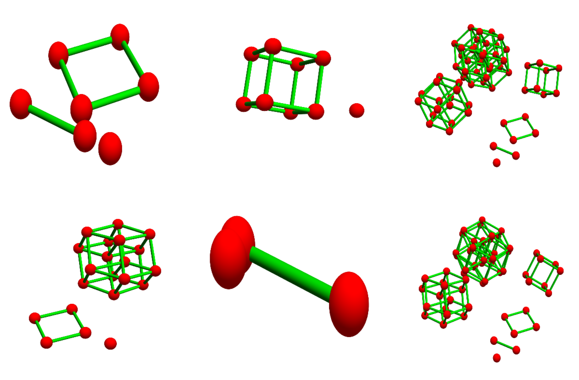
Figure (5) illustrates non-unique factorization in the strong ring It is adapted from [2] in weak ring. The two ring elements and are the same. It is the decomposition , where is a point is an interval . This gives the square , the cube and hyper cube .




Cartesian closed category
15.9.
The goal of this appendix is to see the strong ring of simplicial complexes as a cartesian closed category and to ask whether it is a topos. As we have already finite products, the first requires to show the existence of exponentials. Cartesian closed categories are important in computer science as they have simply typed lambda calculus as language. Also here, we are close to computer science as we deal with a category of objects which (if they are small enough) can be realized in a computer. The elements can be represented as polynomials in a ring for example. We deal with a combinatorial category which can be explored without the need of finite dimensional approximations. It is part of combinatorics as all objects are finite.
15.10.
In order to realize the ring as a category we need to define the morphisms, identifying an initial and terminal object (here and ) and show that currying works: there is an exponential object in the ring such that the set of morphisms from to corresponds to the morphisms via a Curry bijection seeing a graph of a function of two variables as a graph of the function from to functions from to .
15.11.
The existence of a product does not guarantee that a category is cartesian closed. Topological spaces or smooth manifolds are not cartesian closed but compactly generated Hausdorff spaces are. In our case, we are close to the category of finite sets which is cartesian closed. Like for finite sets we are close to computer science as procedures in computer programming languages are using the Curry bijection. Since the object is in general very large, it is as for now more of theoretical interest.
15.12.
The strong ring resembles much the category of sets but there are negative elements in . We can look at the category of finite signed sets which is the subcategory of zero dimensional signed simplicial complexes. Also this is a ring. It is isomorphic to as a ring but the set of morphisms produces a category which has more structure than the ring . This category of signed -dimensional simplicial complexes is Cartesian closed in the same way than the category of sets is. It is illustrative to see the exponential element is th set of all subsets of . But this shows how exponential elements can become large.
15.13.
A simplicial complex as a finite set of non-empty sets, which is closed under the operation of taking non-empty subsets. [The usual definition is to looking at the base set and insisting that is a set of subset of with the property that if and then and also asking that for every . Obviously the first given point-free definition is equivalent. ] There is more structure than just the set of sets as the elements in are partially ordered. A morphism between two simplicial complexes is not just a map between the sets but an order preserving map. This implies that the simplices are mapped into each other. We could rephrase this that a morphism induces a graph homomorphism between the barycentric refinements and but there are more graph homomorphisms in general on .
15.14.
The class of simplicial complexes is a category for which the objects are the simplicial complexes and the morphisms are simplicial functions, functions which preserve simplices. In the point-free definition this means to look at functions from to which preserve the partial order. In order to be close to the definition of continuous functions (the morphisms in topological spaces) or measurable functions (the morphisms in measure spaces) one could ask that is a simplicial complex for every simplicial complex. As can be the empty complex this is fine. [If for some set , the inverse can be empty would not be good since simplicial complexes never contain the empty set. This is fine for the empty complex, which does not contain the empty set neither. But if we look at as a complex by itself, then can be the empty complex. It is in general important to distinguish the elements in the simplicial complex from the subcomplex it represents, evenso this is often not done. ]
15.15.
The category of simplicial complexes is close to the category of finite sets as the morphisms are just a subclass of all functions. There is an other essential difference: the product of two simplicial complexes is not a simplicial complex any more in general, while the product as sets is a set. This is also different from geometric realizations of simplicial complexes (called “polyhedra” in algebraic topology), where the product is a simplicial complex, the geometric realization of the Barycentric refinement of will do.
15.16.
[To compare with topologies O, where continuous maps have the property that for every , morphisms of simplicial complexes have the property for . But only surjective morphisms also have the property that for every , the reason being that can be empty. A continuous map on topological spaces which is also open has the property that and preserve the topology. A constant map for example is in general not open. We see that not only the object of simplicial complex is simpler but also that the morphisms are simpler.] It is better to therefore of a morphism between simplicial complexes as a map for which both and preserve sub simplicial complexes.
15.17.
In order to work within the class of simplicial complexes (actually the special case of Whitney complexes of graphs), we had looked in [17] at the Barycentric refinements of Cartesian products and called this the Cartesian product. We had to live however with the consequence that the product is not associative: already is the Barycentric refinement of . While the geometric realization of the Barycentric refinement is topologically equivalent to , there is a problem with products as in the topological realization meaning that the arithmetic is not compatible. The geometric realization destroys the arithmetic. In the strong ring is a multiplicative prime, in the geometric realization, it is not; it decays as .
15.18.
Having enlarged the category to the strong ring, we have not only to deal with morphisms for simplicial complexes, we also have to say what the morphisms in the ring are. The definition is recursive with respect to the degree of a ring element, where the degree is the degree in the Stanley-Reisner polynomial representation. A map is a morphism, if it is a morphism of simplicial complexes if are simplicial complexes and if for every pair in the ring, there is a pair in the ring and morphisms such that . [By the way, the degree of a monomial in the Stanley-Reisner representation only relates to the dimension if we is prime, that is if is a simplicial complex. In an product , the degree of a monomial is , where is the clique number. It is the clique number which is additive and not the dimension. The monomial in for example belongs to a two-dimensional cell. ]
15.19.
The strong ring is a ring and a category. But it is itself an element in the category of rings. The image of the map is a subring of the Sabidussi ring of all graphs. The map is a ring isomorphism. If we think of as a category, then can be thought so too and is now a functor. This is nothing strange. Category is a universal language where objects of categories can be categories themselves. A directed graph for example is a category, where the objects are the vertices and the morphisms are the directed edges.
15.20.
The strong ring is also a cartesian monodidal category, a category with a notion of tensor product. The unit is the unit in the ring. It is also a finitely complete category, which is a category in which pullbacks exist: given any two ring elements and two morphisms , there is a subcomplex of such that for all , the equation holds. The subcomplex is called a pullback.
15.21.
The strong ring appears also to be a topos but we have not yet checked that. A topos is a cartesian closed category with a sub-object classifier. Examples of topoi are sets or the G-dynamical systems for a group G or the category of sheaves on a topological space. Topoi enjoy stability properties: the fundamental theorem of topos theory tells that a topos is stable under slicing, i.e that it is locally cartesian closed.
References
- [1] B. Grünbaum. Polytopes, graphs, and complexes. Bull. Amer. Math. Soc., 76:1131–1201, 1970.
- [2] R. Hammack, W. Imrich, and S. Klavžar. Handbook of product graphs. Discrete Mathematics and its Applications (Boca Raton). CRC Press, Boca Raton, FL, second edition, 2011. With a foreword by Peter Winkler.
- [3] W. Imrich and S. Klavzar. Product graphs, Structure and recognition. John Wiley and Sons, Inc. New York, 2000.
- [4] D.A. Klain and G-C. Rota. Introduction to geometric probability. Lezioni Lincee. Accademia nazionale dei lincei, 1997.
- [5]
O. Knill.
A graph theoretical Gauss-Bonnet-Chern theorem.
http://arxiv.org/abs/1111.5395, 2011. - [6] O. Knill. A discrete Gauss-Bonnet type theorem. Elemente der Mathematik, 67:1–17, 2012.
- [7]
O. Knill.
A graph theoretical Poincaré-Hopf theorem.
http://arxiv.org/abs/1201.1162, 2012. - [8]
O. Knill.
On index expectation and curvature for networks.
http://arxiv.org/abs/1202.4514, 2012. - [9]
O. Knill.
The McKean-Singer Formula in Graph Theory.
http://arxiv.org/abs/1301.1408, 2012. - [10]
O. Knill.
The theorems of Green-Stokes,Gauss-Bonnet and Poincare-Hopf in Graph
Theory.
http://arxiv.org/abs/1201.6049, 2012. - [11] O. Knill. A Brouwer fixed point theorem for graph endomorphisms. Fixed Point Theory and Applications, 85, 2013.
- [12]
O. Knill.
The Dirac operator of a graph.
http://arxiv.org/abs/1306.2166, 2013. - [13]
O. Knill.
Classical mathematical structures within topological graph theory.
http://arxiv.org/abs/1402.2029, 2014. - [14]
O. Knill.
Curvature from graph colorings.
http://arxiv.org/abs/1410.1217, 2014. - [15]
O. Knill.
The graph spectrum of barycentric refinements.
http://arxiv.org/abs/1508.02027, 2015. - [16]
O. Knill.
The Jordan-Brouwer theorem for graphs.
http://arxiv.org/abs/1506.06440, 2015. - [17]
O. Knill.
The Künneth formula for graphs.
http://arxiv.org/abs/1505.07518, 2015. - [18]
O. Knill.
A Sard theorem for graph theory.
http://arxiv.org/abs/1508.05657, 2015. - [19]
O. Knill.
Universality for barycentric subdivision.
http://arxiv.org/abs/1509.06092, 2015. - [20]
O. Knill.
Gauss-Bonnet for multi-linear valuations.
http://arxiv.org/abs/1601.04533, 2016. - [21]
O. Knill.
On Fredholm determinants in topology.
https://arxiv.org/abs/1612.08229, 2016. - [22]
O. Knill.
On primes, graphs and cohomology.
https://arxiv.org/abs/1608.06877, 2016. - [23]
O. Knill.
Some experiments in number theory.
https://arxiv.org/abs/1606.05971, 2016. - [24]
O. Knill.
On Helmholtz free energy for finite abstract simplicial complexes.
https://arxiv.org/abs/1703.06549, 2017. - [25]
O. Knill.
On the arithemtic of graphs.
https://arxiv.org/abs/1706.05767, 2017. - [26]
O. Knill.
Sphere geometry and invariants.
https://arxiv.org/abs/1702.03606, 2017. - [27]
O. Knill.
A case study in interaction cohomology.
http://www.math.harvard.edu/knill/graphgeometry/papers/interactioncohomology.pdf, March, 18, 2016. - [28] N. Levitt. The Euler characteristic is the unique locally determined numerical homotopy invariant of finite complexes. Discrete Comput. Geom., 7:59–67, 1992.
- [29] H.P. McKean and I.M. Singer. Curvature and the eigenvalues of the Laplacian. J. Differential Geometry, 1(1):43–69, 1967.
- [30] J. Moser. Selected chapters in the calculus of variations. Lectures in Mathematics ETH Zürich. Birkhäuser Verlag, Basel, 2003. Lecture notes by Oliver Knill.
- [31] G. Sabidussi. Graph multiplication. Math. Z., 72:446–457, 1959/1960.
- [32] B. Simon. Trace Ideals and their Applications. AMS, 2. edition, 2010.
- [33] H. Toda. Theory of nonlinear lattices. Springer-Verlag, Berlin, 1981.
- [34] A.A. Zykov. On some properties of linear complexes. (russian). Mat. Sbornik N.S., 24(66):163–188, 1949.