Training Deep AutoEncoders for Collaborative Filtering
Abstract.
This paper proposes a model for the rating prediction task in recommender systems which significantly outperforms previous state-of-the art models on a time-split Netflix data set. Our model is based on deep autoencoder with 6 layers and is trained end-to-end without any layer-wise pre-training. We empirically demonstrate that: a) deep autoencoder models generalize much better than the shallow ones, b) non-linear activation functions with negative parts are crucial for training deep models, and c) heavy use of regularization techniques such as dropout is necessary to prevent overfitting. We also propose a new training algorithm based on iterative output re-feeding to overcome natural sparseness of collaborate filtering. The new algorithm significantly speeds up training and improves model performance. Our code is available at https://github.com/NVIDIA/DeepRecommender.
1. Introduction
Sites like Amazon, Netflix and Spotify use recommender systems to suggest items to users. Recommender systems can be divided into two categories: context-based and personalized recommendations.
Context based recommendations take into account contextual factors such as location, date and time (Adomavicius and Tuzhilin, 2011). Personalized recommendations typically suggest items to users using the collaborative filtering (CF) approach. In this approach the user’s interests are predicted based on the analysis of tastes and preference of other users in the system and implicitly inferring “similarity” between them. The underlying assumption is that two people who have similar tastes, have a higher likelihood of having the same opinion on an item than two randomly chosen people.
In designing recommender systems, the goal is to improve the accuracy of predictions. The Netflix Prize contest provides the most famous example of this problem (Bennett et al., 2007): Netflix held the Netflix Prize to substantially improve the accuracy of the algorithm to predict user ratings for films.
This is a classic CF problem: Infer the missing entries in an matrix, , whose entry describes the ratings given by the th user to the th item. The performance is then measured using Root Mean Squared Error (RMSE).
1.1. Related work
Deep learning (LeCun et al., 2015) has led to breakthroughs in image recognition, natural language understanding, and reinforcement learning. Naturally, these successes fuel an interest for using deep learning in recommender systems. First attempts at using deep learning for recommender systems involved restricted Boltzman machines (RBM) (Salakhutdinov et al., 2007). Several recent approaches use autoencoders (Sedhain et al., 2015; Strub and Mary, 2015), feed-forward neural networks (He et al., 2017) and recurrent recommender networks (Wu et al., 2017). Many popular matrix factorization techniques can be thought of as a form of dimensionality reduction. It is, therefore, natural to adapt deep autoencoders for this task as well. I-AutoRec (item-based autoencoder) and U-AutoRec (user-based autoencoder) are first successful attempts to do so (Sedhain et al., 2015).
There are many non deep learning types of approaches to collaborative filtering (CF) (Breese et al., 1998; Ricci et al., 2011). Matrix factorization techniques, such as alternating least squares (ALS) (Kim and Park, 2008; Koren et al., 2009) and probabilistic matrix factorization (Mnih and Salakhutdinov, 2008) are particularly popular. The most robust systems may incorporate several ideas together such as the winning solution to the Netflix Prize competition (Koren, 2009).
Note that Netflix Prize data also includes temporal signal - time when each rating has been made. Thus, several classic CF approaches has been extended to incorporate temporal information such as TimeSVD++ (Koren, 2010), as well as more recent RNN-based techniques such as recurrent recommender networks (Wu et al., 2017).
2. Model
Our model is inspired by U-AutoRec approach with several important distinctions. We train much deeper models. To enable this without any pre-training, we: a) use “scaled exponential linear units” (SELUs) (Klambauer et al., 2017), b) use high dropout rates, and d) use iterative output re-feeding during training.
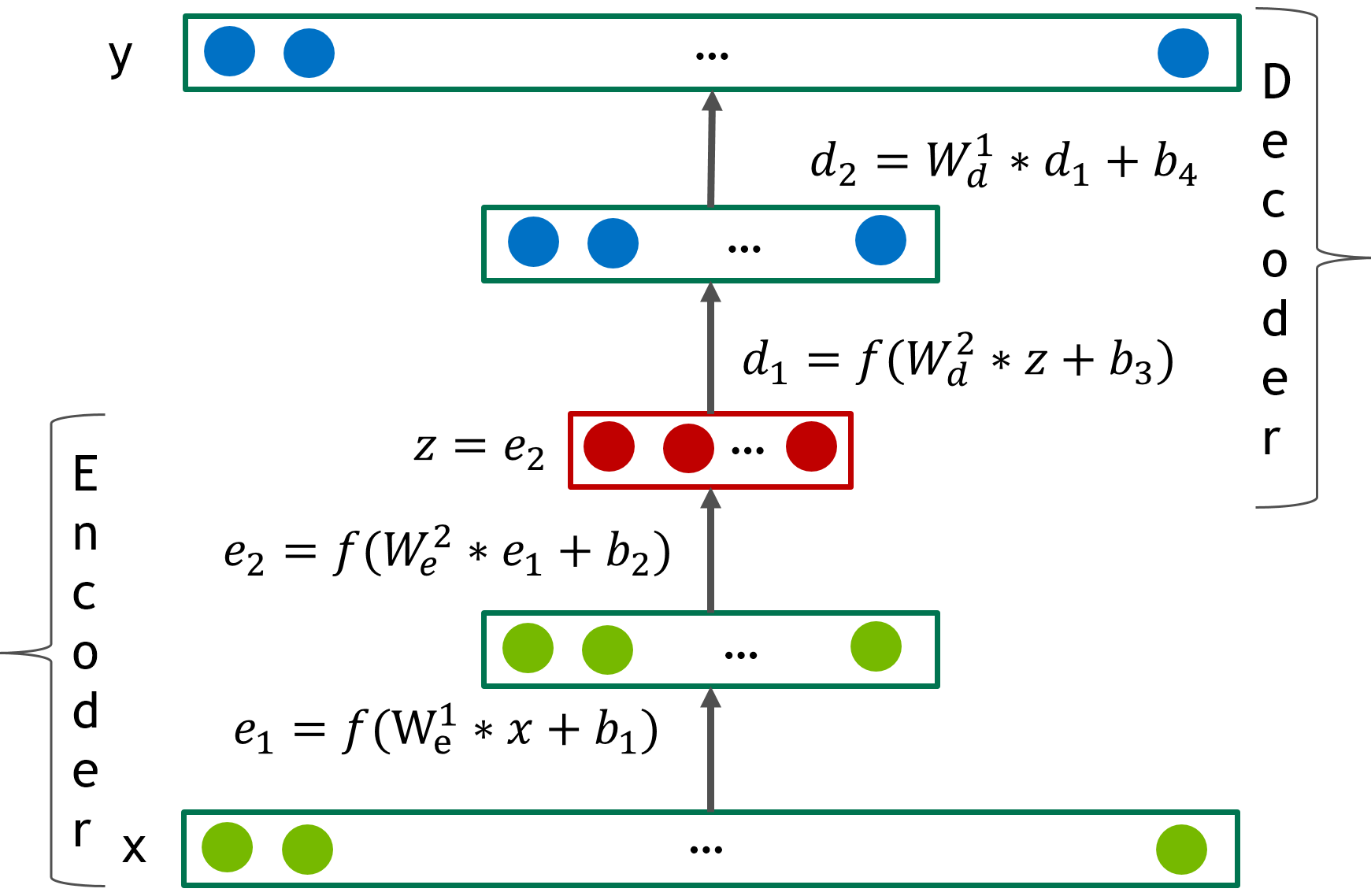
An autoencoder is a network which implements two transformations - encoder and . The “goal” of autoenoder is to obtain dimensional representation of data such that an error measure between and is minimized (Hinton and Zemel, 1994). Figure 1 depicts typical 4-layer autoencoder network. If noise is added to the data during encoding step, the autoencoder is called de-noising. Autoencoder is an excellent tool for dimensionality reduction and can be thought of as a strict generalization of principle component analysis (PCA) (Hinton and Salakhutdinov, 2006). An autoencoder without non-linear activations and only with “code” layer should be able to learn PCA transformation in the encoder if trained to optimize mean squared error (MSE) loss.
In our model, both encoder and decoder parts of the autoencoder consist of feed-forward neural networks with classical fully connected layers computing , where is some non-linear activation function. If range of the activation function is smaller than that of data, the last layer of the decoder should be kept linear. We found it to be very important for activation function in hidden layers to contain non-zero negative part, and we use SELU units in most of our experiments (see Section 3.2 for details).
If decoder mirrors encoder architecture (as it does in our model), then one can constrain decoder’s weights to be equal to transposed encoder weights from the corresponding layer . Such autoencoder is called constrained or tied and has almost two times less free parameters than unconstrained one.
Forward pass and inference. During forward pass (and inference) the model takes user represented by his vector of ratings from the training set , where is number of items. Note that is very sparse, while the output of the decoder, is dense and contains rating predictions for all items in the corpus.
2.1. Loss function
Since it doesn’t make sense to predict zeros in user’s representation vector , we follow the approach from (Sedhain et al., 2015) and optimize Masked Mean Squared Error loss:
| (1) |
where is actual rating, is reconstructed, or predicted rating, and is a mask function such that if else . Note that there is a straightforward relation between RMSE score and MMSE score: .
2.2. Dense re-feeding
During training and inference, an input is very sparse because no user can realistically rate but a tiny fractions of all items. On the other hand, autoencoder’s output is dense. Lets consider an idealized scenario with a perfect . Then and accurately predicts all user’s future ratings for items . This means that if user rates new item (thereby creating a new vector ) then and . Hence, in this idealized scenario, should be a fixed point of a well trained autoencoder: .
To explicitly enforce fixed-point constraint and to be able to perform dense training updates, we augment every optimization iteration with an iterative dense re-feeding steps (3 and 4 below) as follows:
- (1)
Given sparse , compute dense and loss using equation 1 (forward pass)
- (2)
Compute gradients and perform weight update (backward pass)
- (3)
Treat as a new example and compute . Now both and are dense and the loss from equation 1 has all as non-zeros. (second forward pass)
- (4)
Compute gradients and perform weight update (second backward pass)
Steps (3) and (4) can be also performed more than once for every iteration.
3. Experiments and Results
3.1. Experiment setup
For the rating prediction task, it is often most relevant to predict future ratings given the past ones instead of predicting ratings missing at random. For evaluation purposes we followed (Wu et al., 2017) exactly by splitting the original Netflix Prize (Bennett et al., 2007) training set into several training and testing intervals based on time. Training interval contains ratings which came in earlier than the ones from testing interval. Testing interval is then randomly split into Test and Validation subsets so that each rating from testing interval has a 50% chance of appearing in either subset. Users and items that do not appear in the training set are removed from both test and validation subsets. Table 1 provides details on the data sets.
| Full | 3 months | 6 months | 1 year | |
|---|---|---|---|---|
| Training | 12/99-11/05 | 09/05-11/05 | 06/05-11/05 | 06/04-05/05 |
| Users | 477,412 | 311,315 | 390,795 | 345,855 |
| Ratings | 98,074,901 | 13,675,402 | 29,179,009 | 41,451,832 |
| Testing | 12/05 | 12/05 | 12/05 | 06/05 |
| Users | 173,482 | 160,906 | 169,541 | 197,951 |
| Ratings | 2,250,481 | 2,082,559 | 2,175,535 | 3,888,684 |
For most of our experiments we uses a batch size of 128, trained using SGD with momentum of 0.9 and learning rate of 0.001. We used xavier initialization to initialize parameters. Note, that unlike (Strub and Mary, 2015) we did not use any layer-wise pre-training. We believe that we were able to do so successfully because of choosing the right activation function (see Section 3.2).
3.2. Effects of the activation types
To explore the effects of using different activation functions, we tested some of the most popular choices in deep learning : sigmoid, “rectified linear units” (RELU), or RELU6, hyperbolic tangent (TANH), “exponential linear units” (ELU) (Clevert et al., 2015), leaky relu (LRELU) (Xu et al., 2015) , and “scaled exponential linear units” (Klambauer et al., 2017) (SELU) on the 4 layer autoencoder with 128 units in each hidden layer. Because ratings are on the scale from 1 to 5, we keep last layer of the decoder linear for sigmoid and tanh-based models. In all other models activation function is applied in all layers.
We found that on this task ELU, SELU and LRELU perform much better than SIGMOID, RELU, RELU6 and TANH. Figure 2 clearly demonstrates this. There are two properties which seems to separate activations which perform well from those which do not: a) non-zero negative part and b) unbounded positive part. Hence, we conclude, that in this setting these properties are important for successful training. Thus, we use SELU activation units and tune SELU-based networks for performance.

3.3. Over-fitting the data
The largest data set we use for training, “Netflix Full” from Table 1, contains 98M ratings given by 477K users. Number of movies (e.g. items) in this set is . Therefore, the first layer of encoder will have weights, where is number of units in the layer.
For modern deep learning algorithms and hardware this is relatively small task. If we start with single layer encoders and decoders we can quickly overfit to the training data even for as small as 512. Figure 3 clearly demonstrates this. Switching from unconstrained autoencoder to constrained reduces over-fitting, but does not completely solve the problem.

3.4. Going deeper
While making layers wider helps bring training loss down, adding more layers is often correlated with a network’s ability to generalize. In this set of experiments we show that this is indeed the case here. We choose small enough dimensionality () for all hidden layers to easily avoid over-fitting and start adding more layers. Table 2 shows that there is a positive correlation between the number of layers and the evaluation accuracy.
| Number of layers | Evaluation RMSE | params |
|---|---|---|
| 2 | 1.146 | 4,566,504 |
| 4 | 0.9615 | 4,599,528 |
| 6 | 0.9378 | 4,632,552 |
| 8 | 0.9364 | 4,665,576 |
| 10 | 0.9340 | 4,698,600 |
| 12 | 0.9328 | 4,731,624 |
Going from one layer in encoder and decoder to three layers in both provides good improvement in evaluation RMSE (from 1.146 to 0.9378). After that, blindly adding more layers does help, however it provides diminishing returns. Note that the model with single layer in encoder and decoder has 9,115,240 parameters which is almost two times more than any of these deep models while having much worse evauation RMSE (above 1.0).
3.5. Dropout
Section 3.4 shows us that adding too many small layers eventually hits diminishing returns. Thus, we start experimenting with model architecture and hyper-parameters more broadly. Our most promising model has the following architecture: , which means 3 layers in encoder (512,512,1024), coding layer of 1024 and 3 layers in decoder of size 512,512,n. This model, however, quickly over-fits if trained with no regularization. To regularize it, we tried several dropout values and, interestingly, very high values of drop probability (e.g. 0.8) turned out to be the best. See Figure 4 for evaluation RMSE. We apply dropout on the encoder output only, e.g. . We tried applying dropout after every layer of the model but that stifled training convergence and did not improve generalization.

3.6. Dense re-feeding
Iterative dense re-feeding (see Section 2.2) provides us with additional improvement in evaluation accuracy for our 6-layer-model: (referred to as Baseline below). Here each parameter denotes the number of inputs, hidden units, or outputs and is a dropout layer with a drop probability of . Just applying output re-feeding did not have significant impact on the model performance. However, in conjunction with the higher learning rate, it did significantly increase the model performance. Note, that with this higher learning rate (0.005) but without dense re-feeding, the model started to diverge. See Figure 5 for details.

Applying dense re-feeding and increasing the learning rate, allowed us to further improve the evaluation RMSE from 0.9167 to 0.9100. Picking a checkpoint with best evaluation RMSE and computing test RMSE gives as 0.9099, which we believe is significantly better than other methods.
3.7. Comparison with other methods
We compare our best model with Recurrent Recommender Network from (Wu et al., 2017) which has been shown to outperform PMF (Mnih and Salakhutdinov, 2008), T-SVD (Koren, 2010) and I/U-AR (Sedhain et al., 2015) on the data we use (see Table 1 for data description). Note, that unlike T-SVD and RRN, our method does not explicitly take into account temporal dynamics of ratings. Yet, Table 3 shows that it is still capable of outperforming these methods on future rating prediction task. We train each model using only the training set and compute evaluation RMSE for 100 epochs. Then the checkpoint with the highest evaluation RMSE is tested on the test set.
| DataSet | I-AR | U-AR | RRN | DeepRec |
|---|---|---|---|---|
| Netflix 3 months | 0.9778 | 0.9836 | 0.9427 | 0.9373 |
| Netfix Full | 0.9364 | 0.9647 | 0.9224 | 0.9099 |
“Netflix 3 months” has 7 times less training data compared to “Netflix full”, it is therefore, not surprising that the model’s performance is significantly worse if trained on this data alone (0.9373 vs 0.9099). In fact, the model that performs best on “Netflix full” over-fits on this set, and we had to reduce the model’s complexity accordingly (see Table 4 for details).
| DataSet | RMSE | Model Architecture |
|---|---|---|
| Netflix 3 months | 0.9373 | |
| Netflix 6 months | 0.9207 | |
| Netflix 1 year | 0.9225 | |
| Netfix Full | 0.9099 |
4. Conclusion
Deep learning has revolutionized many areas of machine learning, and it is poised do so with recommender systems as well. In this paper we demonstrated how very deep autoencoders can be successfully trained even on relatively small amounts of data by using both well established (dropout) and relatively recent (“scaled exponential linear units”) deep learning techniques. Further, we introduced iterative output re-feeding - a technique which allowed us to perform dense updates in collaborative filtering, increase learning rate and further improve generalization performance of our model. On the task of future rating prediction, our model outperforms other approaches even without using additional temporal signals.
While our code supports item-based model (such as I-AutoRec) we argue that this approach is less practical than user-based model (U-AutoRec). This is because in real-world recommender systems, there are usually much more users then items. Finally, when building personalized recommender system and faced with scaling problems, it can be acceptable to sample items but not users.
References
- Adomavicius and Tuzhilin (2011) Gediminas Adomavicius and Alexander Tuzhilin. 2011. Context-aware recommender systems. In Recommender systems handbook. Springer, 217–253.
- Bennett et al. (2007) James Bennett, Stan Lanning, and Netflix Netflix. 2007. The Netflix Prize. In In KDD Cup and Workshop in conjunction with KDD.
- Breese et al. (1998) John S. Breese, David Heckerman, and Carl Kadie. 1998. Empirical Analysis of Predictive Algorithms for Collaborative Filtering. In Proceedings of the Fourteenth Conference on Uncertainty in Artificial Intelligence (UAI’98). Morgan Kaufmann Publishers Inc., San Francisco, CA, USA, 43–52. http://dl.acm.org/citation.cfm?id=2074094.2074100
- Clevert et al. (2015) Djork-Arné Clevert, Thomas Unterthiner, and Sepp Hochreiter. 2015. Fast and accurate deep network learning by exponential linear units (elus). arXiv preprint arXiv:1511.07289 (2015).
- He et al. (2017) Xiangnan He, Lizi Liao, Hanwang Zhang, Liqiang Nie, Xia Hu, and Tat-Seng Chua. 2017. Neural collaborative filtering. In Proceedings of the 26th International Conference on World Wide Web. International World Wide Web Conferences Steering Committee, 173–182.
- Hinton and Salakhutdinov (2006) Geoffrey E Hinton and Ruslan R Salakhutdinov. 2006. Reducing the dimensionality of data with neural networks. science 313, 5786 (2006), 504–507.
- Hinton and Zemel (1994) Geoffrey E Hinton and Richard S. Zemel. 1994. Autoencoders, Minimum Description Length and Helmholtz Free Energy. In Advances in Neural Information Processing Systems 6, J. D. Cowan, G. Tesauro, and J. Alspector (Eds.). Morgan-Kaufmann, 3–10. http://papers.nips.cc/paper/798-autoencoders-minimum-description-length-and-helmholtz-free-energy.pdf
- Kim and Park (2008) Hyunsoo Kim and Haesun Park. 2008. Nonnegative matrix factorization based on alternating nonnegativity constrained least squares and active set method. SIAM journal on matrix analysis and applications 30, 2 (2008), 713–730.
- Klambauer et al. (2017) Günter Klambauer, Thomas Unterthiner, Andreas Mayr, and Sepp Hochreiter. 2017. Self-Normalizing Neural Networks. arXiv preprint arXiv:1706.02515 (2017).
- Koren (2009) Yehuda Koren. 2009. The bellkor solution to the netflix grand prize. Netflix prize documentation 81 (2009), 1–10.
- Koren (2010) Yehuda Koren. 2010. Collaborative filtering with temporal dynamics. Commun. ACM 53, 4 (2010), 89–97.
- Koren et al. (2009) Yehuda Koren, Robert Bell, and Chris Volinsky. 2009. Matrix factorization techniques for recommender systems. Computer 42, 8 (2009).
- LeCun et al. (2015) Yann LeCun, Yoshua Bengio, and Geoffrey Hinton. 2015. Deep learning. Nature 521, 7553 (2015), 436–444.
- Mnih and Salakhutdinov (2008) Andriy Mnih and Ruslan R Salakhutdinov. 2008. Probabilistic matrix factorization. In Advances in neural information processing systems. 1257–1264.
- Ricci et al. (2011) Francesco Ricci, Lior Rokach, and Bracha Shapira. 2011. Introduction to recommender systems handbook. In Recommender systems handbook. Springer, 1–35.
- Salakhutdinov et al. (2007) Ruslan Salakhutdinov, Andriy Mnih, and Geoffrey Hinton. 2007. Restricted Boltzmann machines for collaborative filtering. In Proceedings of the 24th international conference on Machine learning. ACM, 791–798.
- Sedhain et al. (2015) Suvash Sedhain, Aditya Krishna Menon, Scott Sanner, and Lexing Xie. 2015. Autorec: Autoencoders meet collaborative filtering. In Proceedings of the 24th International Conference on World Wide Web. ACM, 111–112.
- Strub and Mary (2015) Florian Strub and Jérémie Mary. 2015. Collaborative filtering with stacked denoising autoencoders and sparse inputs. In NIPS workshop on machine learning for eCommerce.
- Wu et al. (2017) Chao-Yuan Wu, Amr Ahmed, Alex Beutel, Alexander J. Smola, and How Jing. 2017. Recurrent Recommender Networks. In Proceedings of the Tenth ACM International Conference on Web Search and Data Mining (WSDM ’17). ACM, New York, NY, USA, 495–503. https://doi.org/10.1145/3018661.3018689
- Xu et al. (2015) Bing Xu, Naiyan Wang, Tianqi Chen, and Mu Li. 2015. Empirical evaluation of rectified activations in convolutional network. arXiv preprint arXiv:1505.00853 (2015).