On Resource Pooling and Separation for LRU Caching

In-memory cache processing can greatly expedite data retrieval, since data are kept in Random Access Memory (RAM). In a typical key-value cache system, e.g., Memcached [1, 39, 68], a data item is added to the cache after a client has requested it and failed. When the cache is full, an old data item needs to be evicted to make room for the new one. This selection is determined by the caching algorithm. Different caching algorithms have been proposed [59, 65]. However, due to the cost of tracking access history, often only LRU or its approximations [80], are adopted [9]. The LRU algorithm replaces the data item that has not been used for the longest period of time.

The current engineering practice is to organize servers into pools based on applications and data domains [9, 68, 28]. On a server, the cache space is divided into isolated slabs according to data item sizes [1, 85]. Note that different servers and slabs have separate LRU lists. These solutions have yielded good performance [1, 32, 85], through coarse level control on resource pooling and separation. However, it is not clear whether these rules of thumb are optimal allocations, or whether one can develop simple solutions to further improve the performance.

These facts present a dilemma. On the one hand, multiple request flows benefit from resource pooling. For example, a shared cache space that provides sufficiently high hit ratios for two flows can improve the utilization of the limited RAM space, especially when the two flows contain overlapped common data items so that a data item brought into cache by one flow can be directly used by others. On the other hand, resource separation facilitates capacity planning for different flows and ensures adequate quality of service for each. For example, a dedicated cache space can prevent one flow with a high request rate from evicting too many data items of another competing flow on the same cache [9].

This dilemma only scratches the surface of whether resource pooling or separation is better for caching. Four critical factors complicate the problem and jointly impact the cache miss probabilities (a.k.a. miss ratios), including request rates, overlapped data items across different request flows, data item popularities and their sizes. Depending on the setting, they may lead to different conclusions. Below we demonstrate the complexity of the optimal strategy using three examples, showing that resource pooling can be asymptotically equal to, better or worse than separation, respectively. Consider two independent flows ($1$ and $2$) of requests with Poisson arrivals of rates $\nu_{1}$ and $\nu_{2}$, respectively. The data items of the two flows do not overlap and have unit sizes unless explicitly specified. Their popularities follow truncated Zipf’s distributions, $p^{(1)}_{i}=c_{1}/i^{\alpha_{1}}$ and $p^{(2)}_{j}=c_{2}/j^{\alpha_{2}},1\leq i,j\leq N$, where $i,j$ are the indeces of the data items of flow $1$ and $2$, respectively. For pooling, two flows share the whole cache. For separation, the cache is partitioned into two parts using fractions $u_{1}$ and $u_{2}$, to serve flow $1$ and $2$ separately, $u_{1}+u_{2}=1,u_{1},u_{2}\geq 0$.

When the cache size is small, the optimal separation strategy achieves a better miss probability than resource pooling. However, for large cache sizes, the miss probabilities are indistinguishable. This is not an coincidence, as shown by Theorem 3. Note that the cache sizes take integer values, thus $u_{1}$ varying up and down.

The simulation results in Fig 3 show that resource pooling achieves a smaller miss probability, primarily attributing to self-organization. The optimal static separation ratio in this case is $u_{1}=0.5$ due to symmetry.

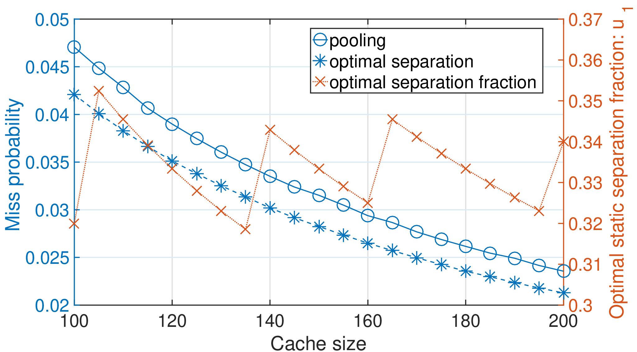
the cache space is small even with equal data item sizes. However, a small cache may not be typical for caching systems. These examples motivate us to systematically study the miss probabilities for competing flows with different rates, distributions, and partially overlapped data items of varying sizes. Our analytical results can be used to explain the puzzling performance differences demonstrated in the previous three examples.

LRU caching is a self-organizing list [3, 2, 22, 23, 38, 52, 70, 54, 5] that has been extensively studied. There are two basic approaches to conduct the analysis: combinatorial and probabilistic. The first approach focuses on the classic amortized [16, 25, 72, 77, 76] and competitive analysis [62, 17, 31, 8, 26, 56]. The second approach includes average case analysis [75, 66, 4] and stochastic analysis [67, 41, 42, 43, 36, 14]. When cache sizes are small, the miss probabilities can be explicitly computed [10, 11, 12, 51]. For large cache sizes, a number of works (e.g., [19, 44, 48, 60, 71]) rely on the Che approximation [29], which has been extended to cache networks [63, 44, 74, 47, 48, 19]. For fluid limits as scaling factors go to infinity (large cache sizes), mean field approximations of the miss probabilities have been developed [55, 81, 50]. For emerging data processing systems, e.g., Memcached [1], since the cache sizes are usually large and the miss probabilities are controlled to be small, it is natural to conduct the asymptotic analysis of the miss probabilities [57, 58]. Although the miss ratios are small, they still significantly impact the caching system performance. Nevertheless, most existing works do not address multiple competing request flows on a shared cache space, which can impact each other through complicated ways.

Workload measurements for caching systems [6, 64, 34, 6, 27, 37, 7, 9] are the basis for theoretical modeling and system optimization. Empirical trace studies show that many characteristics of Web caches can be modeled using power-law distributions [6, 86], including, e.g., the overall data item popularity rank, the document sizes, the distribution of user requests for documents [27, 64, 13, 7], and the write traffic [86]. Similar phenomena have also been found for large-scale key-value stores [9]. These facts motivate us to exploit the heavy-tailed workload characteristics.

Web and network caching is closely related to this study with a large body of dedicated works; see the surveys [82, 69] and the references therein. Recently a utility optimization approach [30, 35] based on the Che approximation [29, 18] has been used to study cache sharing and partitioning. It has concluded that under certain settings the optimal resource separation is better than pooling. However, it is not clear whether the difference is significant or not, especially when the cache size is large for a typical scenario. We show that a simple LRU pooling is asymptotically equivalent to the optimal separation scheme for certain settings, which is significant since the former is adaptive and does not require any configuration or tuning optimization. We focus on the asymptotic miss probabilities for multiple competing flows directly, as the miss ratio is one of the most important metrics for caching systems with large cache sizes in practice.

The miss probability of flow $k$, for a cache size $x$, is represented by a conditional probability ${\mathbb{P}}[C_{0}>x|I_{0}=k]$. Recall $\bar{s}=\sup_{i}s_{i}<\infty$ and that $p^{\circ}_{i}={\mathbb{P}}[R_{0}=d_{i}]$ is defined for the mixed flow. Note $m(z)\to\infty$ as $z\to\infty$. By the theory of regularly varying functions [21], a function $l(x):{\mathbb{R}}^{+}\to{\mathbb{R}}^{+}$ is slowly varying if for any $\lambda>0,l(\lambda x)/l(x)\to 1$ as $x\to\infty$; and $\Phi(x)=x^{\alpha}l(x)$ is called regularly varying of index $\alpha$.

Assume that, for a function $0<\delta(x)\leq 1$ and $\epsilon>0$,

The function $\delta(x)$ characterizes how fast $m^{\leftarrow}(z)$ grows, and thus $\delta(x)$ should be selected to be as large as possible while still satisfying (11). For example, when $m^{\leftarrow}(x)$ is regularly varying, e.g., $m^{\leftarrow}(x)=x^{\beta}$, we can let $\delta(x)=1$, which yields $f(\epsilon)=(1+\epsilon)^{\beta}$. When $m^{\leftarrow}(x)=e^{x^{\xi}},0<\xi<1$, we can pick $\delta(x)=x^{-\xi}$, since $\lim_{x\to\infty}e^{\left(x+\epsilon x^{1-\xi}\right)^{\xi}}/e^{x^{\xi}}=e^{\epsilon\xi}$, implying $f(\epsilon)=e^{\epsilon\xi}$. Both satisfy $\lim_{\epsilon\to 0}f(\epsilon)=1$. Note that in these examples $\delta(x)$ satisfies the following condition: there exist $h_{2}>h_{1}>0,h_{4}>h_{3}>0$ and $x_{0}$, for $x>x_{0}$,

Theorem 1 is the rigorous version of the main result described in (6). The proof is presented in Section VII-B. Based on Theorem 1, we can easily derive some corollaries. We begin with the special case when there is only a single flow $k$ in service and all data items are of the same size $s_{i}\equiv 1$. For a single flow $k$, we simplify the notation by ${\mathbb{P}}\left[R_{0}>x{\big|}I_{0}=k\right]$ $={\mathbb{P}}\left[R_{0}>x\right]$ and ${\mathbb{P}}\left[C_{0}>x{\big|}I_{0}=k\right]={\mathbb{P}}\left[C_{0}>x\right]$. Theorem 1 recovers the results in [57, 58] for Zipf’s distribution

Our result enhances (14) in three aspects. First, we study multiple flows ($p^{(k)}_{i}\neq q^{(k)}_{i}$) that can have overlapped data items and the requested data items can have different sizes. Second, we address the case $\alpha=1$ (then $c$ needs to be replaced by $l(i)$ as in (15)), while the results in [57, 58] assume $\alpha>1$. For $\alpha<1$, we need to assume that only a finite number of data items can be requested (this paper assumes an infinite number); otherwise the popularity distribution does not exist. This special case needs to be handled differently and is not presented in this paper. Due to this difference, the asymptotical result in (13) is only accurate for large $x$ when $\alpha\approx 1$. Third, our result can derive the asymptotic miss probability for a large class of popularity distributions, e.g., Weibull, with varying data item sizes. Corollary 1 extends the results of Theorem 3 in [57] that is proved under the condition (14) to regularly varying probabilities

with $l(\cdot)$ being a slowly varying function, e.g., $l(x)=\log x$.

For multiple request flows without overlapped common data items, we have a decomposition property. Let $P=\left(p^{\circ}_{i},i\geq 1\right)$ be constructed from a set of distributions $Q^{(k)}=\left(q^{(k)}_{i},i\geq 1\right)$ according to probabilities $\nu_{k}$, $\sum_{k}\nu_{k}=1$. Specifically, a random data item following the distribution $P$ is generated by sampling from the distribution $Q^{(k)}$ with a probability $\nu_{k}$. Since two flows $k_{1},k_{2}$ have no overlapped data items, we have ${\mathbb{P}}\left[R_{0}=d^{(k_{1})}_{i}{\big|}I_{0}=k_{2}\right]=0$. Therefore, according to (3), $\left(p^{\circ}_{i},i\geq 1\right)$ can be represented by an unordered list,

Let $\bar{m}(z)=\sum_{i=0}^{\infty}s_{i}\left(1-\exp(-p^{\circ}_{i}z)\right)$. Lemma 1 shows a decomposition property for $m(z)$ and $\bar{m}(z)\sim m(z)$ under certain conditions. Let $m^{(k)}(z)=\sum_{i=0}^{\infty}s^{(k)}_{i}\left(1-\left(1-q^{(k)}_{i}\right)^{z}\right)$ and $\bar{m}^{(k)}(z)=\sum_{i=0}^{\infty}s^{(k)}_{i}\left(1-\exp\left(-q^{(k)}_{i}z\right)\right)$. It is often easier to compute $\bar{m}^{(k)}(z)$ than $m^{(k)}(z)$.

The proof of Lemma 1 is presented in Section VII. It can be used to compute $m(x)$ for multiple flows sharing the same cache. Furthermore, applying Theorem 1, we can derive the miss probability for each flow.

Corollary 3 approximates the miss probabilities for multiple flows with different $\alpha_{k}$ when the cache capacity $x\to\infty$. When the cache capacity is small, this approximation is not accurate. In order to improve the accuracy, denote by $\widetilde{\alpha}_{2}\triangleq\min_{k\in{S_{1}}^{c}}\alpha_{k}$ the second smallest value among all $\alpha_{k}$’s. Defining $S_{2}=\{k\in{\mathbb{Z}}|\alpha_{k}=\widetilde{\alpha}_{2},1\leq k\leq n\}$, we consider all flows in the set $\{k:k\in S_{1}\cup S_{2}\}$, and derive

The inverse function of $m(z)$ can be better approximated by

where $\gamma_{2}=\Gamma(1-1/\widetilde{\alpha}_{2})\sum_{k\in S_{2}}s^{(k)}(c_{k}\nu_{k})^{1/\widetilde{\alpha}_{2}}$ and $\gamma_{1}$ is defined in (28). We obtain more accurate numerical results for miss probabilities using (30) instead of (29) especially when the cache capacity is small, though the expressions in (29) and (30) are asymptotically equivalent. Experiments V in Section V validates this approximation. Alternatively, we also resort to numerical methods to directly evaluate $m^{\leftarrow}(z)$ for more complex cases.

The miss probability of LRU algorithm has been extensively studied using the Che approximation [29]. Now we show that the Che approximation is asymptotically accurate under certain conditions; see a related validity argument in [79]. For multiple flows, the overall miss probability computed by the Che approximation is

where $T$ is the cache characteristic time as the unique solution to $\sum_{i=1}^{\infty}s_{i}(1-e^{-p_{i}^{\circ}T})=x$.

References

- [1] Memcached. http://memcached.org/.
- [2] S. Albers and J. Westbrook. Self organizing data structures. Online Algorithms: The state of the art, 1442:13–41, 1998.
- [3] B. Allen and I. Munro. Self-organizing binary search trees. Journal of the ACM, 25:526–535, 1978.
- [4] N. Alon and J. Spencer. The probabilistic method. John Wiley, 2nd edition, 2000.
- [5] S. Ar, B. Chazelle, and A. Tal. Self-customized bsp trees for collision detection. Computational Geometry: Theory and Applications, 10:23–29, 2000.
- [6] M. Arlitt and L. W. C. Internet web servers: Workload characterization and performance implications. In IEEE/ACM Transaction on Networking, October 1997.
- [7] M. Arlitt, R. Friedrich, and T. Jin. Workload characterization of a web proxy in a cable modem environment. SIGMETRICS Performance Evalation Review, 27(2):25–36, Sept. 1999.
- [8] S. Arora, D. Karger, and M. Karpinski. Polynomial time approximation schemes for dense instances of NP-hard problems. In Proceedings of the 27th STOC, pages 284–293, 1995.
- [9] B. Atikoglu, Y. Xu, E. Frachtenberg, S. Jiang, and M. Paleczny. Workload analysis of a large-scale key-value store. SIGMETRICS Perform. Eval. Rev., 40(1):53–64, June 2012.
- [10] O. I. Aven, L. B. Boguslavsky, and Y. A. Kogan. Some results on distribution-free analysis of paging algorithms. IEEE Trans. Computers, 25(7):737–745, 1976.
- [11] O. I. Aven, E. G. Coffman, and Y. A. Kogan. Stochastic analysis of computer storage, volume 38. Springer Science & Business Media, 1987.
- [12] O. Babaoglu and D. Ferrari. Two-level replacement decisions in paging. IEEE Transactions on Computers, 100(32), 1983.
- [13] P. Barford, A. Bestavros, A. Bradley, and M. Crovella. Changes in web client access patterns. In World Wide Web Journal, Special Issue on Characterization and Performance Evaluation, 1999.
- [14] J. Barrera and C. Paroissin. On the distribution of the search cost for the move-to-front rule with random weights. Journal of Applied Probability, 41(1):250–262, 03 2004.
- [15] S. L. Bell and R. J. Williams. Dynamic scheduling of a system with two parallel servers in heavy traffic with resource pooling: asymptotic optimality of a threshold policy. The Annals of Applied Probability, 11(3):608–649, 08 2001.
- [16] J. Bentley and C. McGeoch. Amortized analysis of self-organizing sequential search heuristics. Communications of the ACM, 28:404–411, 1985.
- [17] J. L. Bentley and C. C. McGeoch. Amortized analyses of self-organizing sequential search heuristics. Communications of the ACM, 28(4):404–411, Apr. 1985.
- [18] D. S. Berger, P. Gland, S. Singla, and F. Ciucu. Exact analysis of TTL cache networks. In 32nd International symposium on Computer Performance, modeling, measurements, and evaluation (IFIP Performance’14), pages 2–23, Turin, Italy, October 2014.
- [19] D. S. Berger, P. Gland, S. Singla, and F. Ciucu. Exact analysis of ttl cache networks. Performance Evaluation, 79:2–23, 2014.
- [20] D. S. Berger, S. Henningsen, F. Ciucu, and J. B. Schmitt. Maximizing cache hit ratios by variance reduction. SIGMETRICS Perform. Eval. Rev., 43(2):57–59, Sept. 2015.
- [21] N. H. Bingham, C. M. Goldie, and J. L. Teugels. Regular Variation. Cambridge University Press, 1987.
- [22] J. Bitner. Heuristics that dynamically organize data structures. SIAM Journal on Computing, 8:82–110, 1979.
- [23] A. Blum, S. Chawla, and A. Kalai. Static optimality and dynamic search-optimality in lists and trees. In Proceedings of the 13th SODA, pages 1–8, 2002.
- [24] C. Borgs, J. T. Chayes, S. Doroudi, M. Harchol-Balter, and K. Xu. The optimal admission threshold in observable queues with state dependent pricing. Probability in the Engineering and Informational Sciences, 28(1):101–119, 12 2013.
- [25] A. Borodin and R. El-Yaniv. Online Computation and Competitive Analysis. Cambridge University Press, New York, NY, USA, 1998.
- [26] A. Borodin, P. Raghavan, S. Irani, and B. Schieber. Competitive paging with locality of reference. In Proceedings of the Twenty-third Annual ACM Symposium on Theory of Computing, STOC ’91, pages 249–259, 1991.
- [27] L. Breslau, P. Cao, L. Fan, G. Phillips, and S. Shenker. Web caching and zipf-like distributions: evidence and implications. In Proceedings of the 18th Conference on Information Communications, 1999.
- [28] N. Bronson, Z. Amsden, G. Cabrera, P. Chakka, P. Dimov, H. Ding, J. Ferris, A. Giardullo, S. Kulkarni, H. Li, M. Marchukov, D. Petrov, L. Puzar, Y. J. Song, and V. Venkataramani. TAO: Facebook’s distributed data store for the social graph. In Proceedings of the 2013 USENIX Conference on Annual Technical Conference, USENIX ATC’13, pages 49–60, Berkeley, CA, USA, 2013. USENIX Association.
- [29] H. Che, Y. Tung, and Z. Wang. Hierarchical web caching systems: modeling, design and experimental results. IEEE Journal on Selected Areas in Communications, 20(7):1305–1314, Sep 2002.
- [30] W. Chu, M. Dehghan, D. Towsley, and Z.-L. Zhang. On allocating cache resources to content providers. In Proceedings of the 2016 conference on 3rd ACM Conference on Information-Centric Networking, pages 154–159. ACM, 2016.
- [31] F. R. Chung, D. J. Hajela, and P. D. Seymour. Self-organizing sequential search and hilbert’s inequalities. In Proceedings of the Seventeenth Annual ACM Symposium on Theory of Computing, STOC ’85, pages 217–223, 1985.
- [32] A. Cidon, A. Eisenman, M. Alizadeh, and S. Katti. Cliffhanger: Scaling performance cliffs in web memory caches. In USENIX NSDI, pages 379–392, 2016.
- [33] E. G. Coffman, Jr. and P. J. Denning. Operating Systems Theory. Prentice Hall Professional Technical Reference, 1973.
- [34] C. Cunha, A. Bestavros, and M. Crovella. Characteristics of WWW client-based traces. Technical report, Boston University, Boston, MA, USA, 1995.
- [35] M. Dehghan, W. Chu, P. Nain, and D. Towsley. Sharing LRU cache resources among content providers: A utility-based approach. arXiv preprint arXiv:1702.01823, 2017.
- [36] R. P. Dobrow and J. A. Fill. The move-to-front rule for self-organizing lists with markov dependent requests. In Discrete Probability and Algorithms, pages 57–80, New York, NY, 1995. Springer New York.
- [37] B. M. Duska, D. Marwood, and M. J. Feely. The measured access characteristics of world-wide-web client proxy caches. In Proceedings of the USENIX Symposium on Internet Technologies and Systems (USITS ’97), December 1999.
- [38] V. Estivill-Castro and D. Wood. A survey of adaptive sorting algorithms. ACM Computing Surveys, 24:441–476, 1992.
- [39] B. Fan, D. G. Andersen, and M. Kaminsky. MemC3: Compact and concurrent MemCache with dumber caching and smarter hashing. In Proceedings of the 10th USENIX Conference on Networked Systems Design and Implementation, NSDI’13, pages 371–384, Lombard, IL, 2013. USENIX Association.
- [40] A. Ferragut, I. Rodriguez, and F. Paganini. Optimizing TTL caches under heavy-tailed demands. SIGMETRICS Perform. Eval. Rev., 44(1):101–112, June 2016.
- [41] J. Fill. An exact formula for the move-to-front rule for self-organizing lists. Journal of Theoretical Probability, 9(1):113–160, 1996.
- [42] J. A. Fill. Limits and rates of convergence for the distribution of search cost under the move-to-front rule. Theoretical Computer Science, 164(1):185 – 206, 1996.
- [43] P. Flajolet, D. Gardy, and L. Thimonier. Birthday paradox, coupon collectors, caching algorithms and self-organizing search. Discrete Applied Mathematics, 39(3):207–229, November 1992.
- [44] N. C. Fofack, P. Nain, G. Neglia, and D. Towsley. Analysis of TTL-based cache networks. In Performance Evaluation Methodologies and Tools (VALUETOOLS), 2012 6th International Conference on, pages 1–10. IEEE, 2012.
- [45] N. C. Fofack, P. Nain, G. Neglia, and D. Towsley. Performance evaluation of hierarchical TTL-based cache networks. Computer Networks, 65:212 – 231, 2014.
- [46] C. Fricker, P. Robert, and J. Roberts. A versatile and accurate approximation for LRU cache performance. In Proceedings of the 24th International Teletraffic Congress, ITC ’12, pages 8:1–8:8, 2012.
- [47] M. Gallo, B. Kauffmann, L. Muscariello, A. Simonian, and C. Tanguy. Performance evaluation of the random replacement policy for networks of caches. Performance Evaluation, 72:16–36, 2014.
- [48] M. Garetto, E. Leonardi, and V. Martina. A unified approach to the performance analysis of caching systems. ACM Transactions on Modeling and Performance Evaluation of Computing Systems, 1(3):12, 2016.
- [49] N. Gast and B. Van Houdt. Transient and steady-state regime of a family of list-based cache replacement algorithms. In Proceedings of the 2015 ACM SIGMETRICS International Conference on Measurement and Modeling of Computer Systems, SIGMETRICS ’15, pages 123–136, 2015.
- [50] N. Gast and B. Van Houdt. Transient and steady-state regime of a family of list-based cache replacement algorithms. ACM SIGMETRICS Performance Evaluation Review, 43(1):123–136, 2015.
- [51] E. Gelenbe. A unified approach to the evaluation of a class of replacement algorithms. IEEE Transactions on Computers, 100(6):611–618, 1973.
- [52] G. Gonnet, J. Munro, and H. Suwanda. Exegesis of self-organizing linear search. SIAM Journal on Computing, 10:613–637, 1981.
- [53] J. M. Harrison and M. J. López. Heavy traffic resource pooling in parallel server systems. Queueing Systems, 33(4):339–368, 1999.
- [54] J. Hester and D. Hirschberg. Self-organizing linear search. ACM Computing Surveys, 17:295–311, 1985.
- [55] R. Hirade and T. Osogami. Analysis of page replacement policies in the fluid limit. Operations research, 58(4-part-1):971–984, 2010.
- [56] S. Irani, A. R. Karlin, and S. Phillips. Strongly competitive algorithms for paging with locality of reference. In Proceedings of the Third Annual ACM-SIAM Symposium on Discrete Algorithms, SODA ’92, pages 228–236, Philadelphia, PA, USA, 1992. Society for Industrial and Applied Mathematics.
- [57] P. R. Jelenković. Asymptotic approximation of the move-to-front search cost distribution and least-recently-used caching fault probabilities. The Annals of Applied Probability, (2):430–464, 1999.
- [58] P. R. Jelenković and A. Radovanović. Least-recently-used caching with dependent requests. Theoretical Computer Science, 326(1-3):293–327, Oct. 2004.
- [59] S. Jiang and X. Zhang. LIRS: An efficient low inter-reference recency set replacement policy to improve buffer cache performance. In Proceedings of the 2002 ACM SIGMETRICS International Conference on Measurement and Modeling of Computer Systems, SIGMETRICS ’02, pages 31–42, New York, NY, USA, 2002. ACM.
- [60] J. Jung, A. W. Berger, and H. Balakrishnan. Modeling TTL-based Internet Caches. In IEEE Infocom 2003, San Francisco, CA, April 2003.
- [61] O. Kella. The threshold policy in the M/G/1 queue with server vacations. Naval Research Logistics (NRL), 36(1):111–123, 1989.
- [62] D. E. Knuth. The Art of Computer Programming, Volume 3: (2Nd Ed.) Sorting and Searching. Addison Wesley Longman Publishing Co., Inc., Redwood City, CA, USA, 1998.
- [63] N. Laoutaris, H. Che, and I. Stavrakakis. The LCD interconnection of LRU caches and its analysis. Performance Evaluation, 63(7):609–634, 2006.
- [64] S. Manley and M. Seltzer. Web facts and fantasy. In Proceedings of the USENIX Symposium on Internet Technologies and Systems, December 1997.
- [65] N. Megiddo and D. S. Modha. ARC: A self-tuning, low overhead replacement cache. In Proceedings of the 2Nd USENIX Conference on File and Storage Technologies, FAST ’03, pages 115–130, Berkeley, CA, USA, 2003. USENIX Association.
- [66] R. Motwani. Average-case analysis of algorithm for matching and related problems. Journal of the ACM, 41:1329–1356, 1994.
- [67] P. R. Nelson. Single-shelf library-type markov chains with infinitely many books. Journal of Applied Probability, pages 298–308, 1977.
- [68] R. Nishtala, H. Fugal, S. Grimm, M. Kwiatkowski, H. Lee, H. C. Li, R. McElroy, M. Paleczny, D. Peek, P. Saab, D. Stafford, T. Tung, and V. Venkataramani. Scaling memcache at facebook. In Presented as part of the 10th USENIX Symposium on Networked Systems Design and Implementation (NSDI 13), pages 385–398, Lombard, IL, 2013. USENIX.
- [69] S. Podlipnig and L. Böszörmenyi. A survey of web cache replacement strategies. ACM Computing Surveys (CSUR), 35(4):374–398, Dec. 2003.
- [70] R. Rivest. On self-organizing sequential search heuristics. Communications of the ACM, 19:63–67, 1976.
- [71] J. Roberts and N. Sbihi. Exploring the memory-bandwidth tradeoff in an information-centric network. In Teletraffic Congress (ITC), 2013 25th International, pages 1–9. IEEE, 2013.
- [72] L. Roditty and U. Zwick. A fully dynamic reachability algorithm for directed graphs with an almost linear update time. In Proceedings of the 36th STOC, pages 184–191, 2004.
- [73] E. J. Rosensweig, J. Kurose, and D. Towsley. Approximate models for general cache networks. In Proceedings of the 29th Conference on Information Communications, INFOCOM’10, pages 1100–1108, San Diego, California, USA, 2010. IEEE Press.
- [74] E. J. Rosensweig, J. Kurose, and D. Towsley. Approximate models for general cache networks. In INFOCOM, 2010 Proceedings IEEE, pages 1–9. IEEE, 2010.
- [75] A. S. and M. Mitzenmacher. Average case analyses of list update algorithms. Algorithmica, 21:312–329, 1998.
- [76] D. Sleator and R. Tarjan. Amortized efficiency of list update and paging rules. Communications of the ACM, 28:202–208, 1985.
- [77] D. Sleator and R. Tarjan. Self-adjusting binary search trees. Journal of the ACM, 32:652–686, 1985.
- [78] A. L. Stolyar. Maxweight scheduling in a generalized switch: State space collapse and workload minimization in heavy traffic. The Annals of Applied Probability, 14(1):1–53, 02 2004.
- [79] J. Tan, L. Zhang, and Y. Wang. Miss behavior for caching with lease. SIGMETRICS Performance Evaluation Review, MAMA workshop, 43(2):60–62, 2015.
- [80] A. S. Tanenbaum. Modern Operating Systems. Prentice Hall Press, Upper Saddle River, NJ, USA, 2rd edition, 2001.
- [81] N. Tsukada, R. Hirade, and N. Miyoshi. Fluid limit analysis of fifo and rr caching for independent reference models. Performance Evaluation, 69(9):403–412, 2012.
- [82] J. Wang. A survey of web caching schemes for the internet. SIGCOMM Computer Communication Review, 29(5):36–46, Oct. 1999.
- [83] X. Wu, L. Zhang, Y. Wang, Y. Ren, M. Hack, and S. Jiang. zExpander: A key-value cache with both high performance and fewer misses. In Proceedings of the Eleventh European Conference on Computer Systems, EuroSys ’16, pages 14:1–14:15, New York, NY, USA, 2016. ACM.
- [84] Y. Xu, E. Frachtenberg, S. Jiang, and M. Paleczny. Characterizing facebook’s memcached workload. IEEE Internet Computing, 18(2):41–49, 2014.
- [85] Y. Xua, E. Frachtenbergb, and S. Jiang. Building a high-performance key-value cache as an energy-efficient appliance. Performance Evaluation, 79:24–37, September 2014.
- [86] Y. Yang and J. Zhu. Write skew and zipf distribution: Evidence and implications. ACM Transactions on Storage (TOS), 12(4):21:1–21:19, June 2016.