Tight-binding methods for general longitudinally driven photonic lattices – edge states and solitons

Mark J. Ablowitz and Justin T. Cole Affiliation: Department of Applied Mathematics, University of Colorado, Boulder, Colorado 80309

August 24, 2026

Abstract

A systematic approach for deriving tight-binding approximations in general longitudinally driven lattices is presented. As prototypes, honeycomb and staggered square lattices are considered. Time-reversal symmetry is broken by varying/rotating the waveguides, longitudinally, along the direction of propagation. Different sublattice rotation and structure are allowed. Linear Floquet bands are constructed for intricate sublattice rotation patterns such as counter rotation, phase offset rotation, as well as different lattice sizes and frequencies. An asymptotic analysis of the edge modes, valid in a rapid-spiraling regime, reveals linear and nonlinear envelopes which are governed by linear and nonlinear Schrödinger equations, respectively. Nonlinear states, referred to as topologically protected edge solitons are unidirectional edge modes. Direct numerical simulations for both the linear and nonlinear edge states agree with the asymptotic theory. Topologically protected modes are found; they possess unidirectionality and do not scatter at lattice defect boundaries.

PACS numbers: 42.65.Tg, 42.65.Jx, 42.82.Et

pacs

Valid PACS appear here

I Introduction

In recent years the study of topological edge/interface and surface modes has been a very active area of research. Fundamental research in systems where time-reversal symmetry is broken have been found to support unidirectional edge modes that remain intact over long distance and against defects; these systems include magneto-optics [1, 2], photonics [3, 4, 5] and acoustics [6]. While these systems have very different underlying physics they all share some common properties; they have a boundary that separates two distinct regions. A boundary discontinuity alone can be enough to support edge states, but to generate topologically protected modes in these systems typically time-reversal symmetry must be broken. The manner in which this is accomplished is different for each system; here however we focus on optical beams propagating through longitudinally driven waveguide arrays.

Some of the recent advances in topologically protected systems include: PT symmetry crystals [7], bi-anisotropic metamaterials [8, 9] and surface plasmons [10]. Higher-dimensional systems have also been examined [11], where the 3D analog of Dirac points called Weyl points have been reported [12, 13]. Quasi-crystal type arrays can also support unidirectional edge states [14].

In photonic lattices, regions of high refractive index can be etched into bulk silica using femtosecond laser etching techniques [15, 16] and act as waveguides for the beam. One way to break time-reversal symmetry is to rotate these waveguides longitudinally, creating an array configuration that changes along along the direction of beam propagation. Such lattices, which are orthogonal to the direction of the beam propagation, have been constructed at optical frequencies and topologically protected edge modes have been experimentally observed [5].

One of the special features topological edge modes exhibit is their one-way scatter-free motion even when lattice defects are encountered. Such traveling modes are said to be topologically protected meaning that unidirectionality is preserved even under significant deformations of the lattice. Topological invariants, such as Chern number [17] or Zak phase [18], can be associated with these topological modes. The robust nature of topologically protected edge modes suggests that they will be useful in many applications where small imperfections are always present.

Photonic lattices that can support linear edge modes include honeycomb [5] and staggered square lattices [19, 20] each of which has two lattice sites per unit cell. We refer to any lattice with two or more sites in a unit cell as non-simple. In this work we provide a direct route for deriving tight-binding equations that describe beam propagation in general longitudinally varying lattices with either simple or non-simple configurations. As typical examples we analyze honeycomb and staggered square lattices, though more complex lattices can be considered within the framework we present. In doing so, we are able to study a wide range of lattice dynamics including periodic but non-synchronized (out of phase) waveguide motion with phase offset across the two sublattices or counter rotating lattices etc. The Floquet bands are associated with intriguing edge mode dynamics which include: flat (stationary), non-unidirectional, oscillatory, and simultaneous topological and non-topological eigenstates. These modes complement the well-known traveling edge states present when the lattice waveguides rotate in-phase with each other.

For a particular rotation pattern we find common structure in the dispersion bands of both the honeycomb and staggered square lattices. This suggests that for a particular waveguide rotation there is an associated edge wave dynamic that is independent of the underlying lattice configuration. Additionally, our tight-binding model incorporates the geometry of the individual waveguides. When the waveguides are stretched in a preferred direction we find non-topologically protected modes whose edge modes reflect at lattice defects, rather than simply moving around the defect like a protected mode.

We present an asymptotic analysis which reveals that along the lattice boundary the edge modes can behave as one-dimensional solutions to the nonlinear Schrödinger (NLS) equation. Hence we refer to these traveling modes as edge solitons, where applicable. The NLS equation is a universal model for the envelope description of dispersive waves in weakly-nonlinear media, like the systems we consider in this paper. The nonlinear edge mode envelope can be seen as a balance between the lattice induced linear dispersion effects and sufficiently strong beam focusing or defocusing. Indeed, many properties associated with the NLS equation can be found in photonic topological insulators, such as modulational instability [21], band gap solitons [22] and soliton propagation in helically driven photonic graphene [23]. Moreover, we construct nonlinear modes that, to leading order, satisfy the focusing NLS equation and whose corresponding linear dispersion is topologically protected. These modes travel stably around defects. Hence we term these solutions topologically protected edge solitons.

The outline of the paper is as follows. In Sec. II we derive a tight-binding model that describes paraxial beams in general longitudinally driven honeycomb and staggered square lattices. The linear dispersion bands for one-dimensional edge states are computed via Floquet theory in Sec. III. Here we study several complex sublattice rotation patterns and their effect on the edge mode dynamics. In Sec. IV we consider nonlinear edge beams. Both linear and nonlinear edge modes are found to be modulated by a slowly-varying envelope function that satisfy the linear and nonlinear Schrödinger equations, respectively. In the nonlinear regime an asymptotic analysis shows that edge solitons exist for solutions with narrow spectral support around some central frequency. The edge wave behavior across lattice defects is explored in Sec. V. There we observe topologically protected modes to be scatter-free at lattice barriers, in contrast to non-topologically protected modes. We conclude in Sec. VI.

II Derivation of Tight-binding Approximation

Nonlinear quasi-monochromatic light beams propagating through photonic lattices are described by the paraxial wave or nonlinear Schrödinger (NLS) equation

i\frac{\partial\psi}{\partial z}+\frac{1}{2k_{0}}\nabla^{2}\psi-\frac{k_{0}}{n_{0}}\left(\Delta n({\bf r},z)+n_{2}|\psi|^{2}\right)\psi=0\;,

(1)

where $\nabla^{2}\equiv\partial_{x}^{2}+\partial_{y}^{2}$ and $\psi({\bf r},z)$ is a complex envelope function defined on the transverse plane ${\bf r}=(x,y)$ and propagation direction $z$ . The function $\Delta n({\bf r},z)$ is the lattice potential and it models the variations in the refractive index. The physical parameters are the wavenumber $k_{0}=2\pi n_{0}/\lambda$ , bulk index of refraction $n_{0}$ , beam wavelength $\lambda$ , deviation from bulk index $|\Delta n|,$ and Kerr coefficient $n_{2}.$

We may think of a lattice with two generating sites per unit cell as the combination of two interpenetrating sublattices with potentials $V_{1}({\bf r})$ and $V_{2}({\bf r})$ . These two sublattices have regions of high refractive index concentrated at the white and black lattice sites, respectively, as shown in Figs. 1 and 2. To model such a lattice configuration we employ the potential function

\Delta n({\bf r})=|\Delta n|\left[1-V_{1}({\bf r})-V_{2}({\bf r})\right]\;,

(2)

that consists of well-localized dips (minima) located at the lattice sites. We approximate these sublattices by the sum of Gaussians

		$\displaystyle V_{1}({\bf r})=\sum_{{\bf r}_{j}\in\mathcal{W}}\tilde{V}({\bf r}-{\bf r}_{j})\;,~~~V_{2}({\bf r})=\sum_{{\bf r}_{k}\in\mathcal{B}}\tilde{V}({\bf r}-{\bf r}_{k})\;,$		(3)
		$\displaystyle~~~~~~~~~\tilde{V}({\bf r})=\exp{\left(-\frac{x^{2}}{\sigma_{x}^{2}}-\frac{y^{2}}{\sigma_{y}^{2}}\right)}\;~~~~\sigma_{x},\sigma_{y}>0\;,$

where the positions of the white and black lattice sites are given, respectively, by the sets

\mathcal{W}=\left\{{\bf r}_{j}:V_{1}({\bf r}_{j})=1\right\}~,~~~\mathcal{B}=\left\{{\bf r}_{k}:V_{2}({\bf r}_{k})=1\right\}.

Asymmetry in the waveguide geometry can be explored by adjusting the width parameters $\sigma_{x}$ and $\sigma_{y}.$ When $\sigma_{x}=\sigma_{y}$ we say the lattice isotropic, whereas when $\sigma_{x}\not=\sigma_{y}$ the lattice is anisotropic. Detuning (difference in the refractive index) between the sublattices can approximated by including a coefficient $0<q<1$ in front of one of the sublattice potentials i.e. $V_{2}({\bf r})\rightarrow qV_{2}({\bf r})$ . Investigations of detuned lattices is beyond the scope of this paper and we do not consider it here. We point out that this approach can be readily extended to lattices with more than two lattice sites per unit cell by adding an additional sublattice $V_{3}({\bf r})$ function to potential function (2) that is defined similar to Eq. (3).

For well-separated lattice sites, and when ${\bf r}$ is near ${\bf r}_{j}$ or ${\bf r}_{k}$ , the potential function (2) is approximated by the first few terms of its Taylor series and thus takes a paraboloid form, namely

\Delta n({\bf r})\approx|\Delta n|\left(\frac{x^{2}}{\sigma_{x}^{2}}+\frac{y^{2}}{\sigma_{y}^{2}}\right)\;,~{\rm as~}{\bf r}\rightarrow{\bf r}_{j},{\bf r}_{k}\;.

(4)

The orbital functions used to construct the ansatz in Eq. (11) are normalized Gaussians centered at the lattice sites and satisfy a linear Schrödinger equation with potential function of the form in Eq. (4).

To break time-reversal symmetry the two sublattices $V_{1}({\bf r})$ and $V_{2}({\bf r})$ are rotated according to the functions ${\bf h}_{1}(z),{\bf h}_{2}(z)$ , respectively, i.e.

\Delta n({\bf r},z)=|\Delta n|\bigg[1-V_{1}({\bf r}-{\bf h}_{1}(z))-V_{2}({\bf r}-{\bf h}_{2}(z))\bigg]\;.

The only restrictions we place upon the functions ${\bf h}_{1}(z),{\bf h}_{2}(z)$ is that they are smooth. This is quite general. Since most researchers have studied periodic longitudinal variation, below we will assume ${\bf h}_{1}(z),{\bf h}_{2}(z)$ are periodic; but they need not be so. In particular, we take

{\bf h}_{i}(z)=R_{i}\left(\cos\left(\Omega_{i}z+\chi_{i}\right),\sin\left(\Omega_{i}z+\chi_{i}\right)\right)\;,~i=1,2

(5)

where $R_{i}$ is the helix radius, $\Omega_{i}$ is the angular frequency of the oscillation, and $\chi_{i}$ a phase shift.

Next we move into a coordinate frame co-moving with with the $V_{1}({\bf r},z)$ sublattice by performing the change of variable

{\bf r}^{\prime}={\bf r}-{\bf h}_{1}(z)~~~,~~~z^{\prime}=z\;,

which (after the prime notation is dropped) gives the equation

i\frac{\partial\psi}{\partial z}-i{\bf h}_{1}^{\prime}(z)\cdot\nabla\psi+\frac{1}{2k_{0}}\nabla^{2}\psi-\frac{k_{0}}{n_{0}}\left(\Delta n({\bf r},z)+n_{2}|\psi|^{2}\right)\psi=0\;.

(6)

Introducing the phase transformation

\psi({\bf r},z)=\tilde{\psi}({\bf r},z)\exp\left(\frac{-i\int_{0}^{z}|{\bf A}(\zeta)|^{2}d\zeta}{2}\right)\;,

for the pseudo-field defined by ${\bf A}(z)=-k_{0}{\bf h}^{\prime}_{1}(z)$ yields (after dropping the tilde notation)

i\frac{\partial\psi}{\partial z}+\frac{1}{2k_{0}}\left(\nabla+i{\bf A}(z)\right)^{2}\psi-\frac{k_{0}}{n_{0}}\left(\Delta n({\bf r},z)+n_{2}|\psi|^{2}\right)\psi=0\;.

(7)

We non-dimensionalize by

		$\displaystyle x=lx^{\prime}~,~y=ly^{\prime}~,~z=z_{*}z^{\prime}~,$
	$\displaystyle\sigma_{x}$	$\displaystyle=l\sigma_{x}^{\prime}~,~\sigma_{y}=l\sigma_{y}^{\prime}~,~\psi=\sqrt{I_{*}}\psi^{\prime}~,$

where $l$ is the distance between nearest-neighbor lattice sites, $z_{*}=2k_{0}l^{2}$ is the characteristic propagation distance, $I_{*}$ is the peak input beam intensity, nonlinearity coefficient $\sigma=2\gamma k_{0}l^{2}I_{*}$ and lattice amplitude $V_{0}^{2}=2k_{0}^{2}l^{2}|\Delta n|/n_{0}$ . Dropping the ^′ notation, these rescalings give the dimensionless equation

i\frac{\partial\psi}{\partial z}+\left(\nabla+i{\bf A}(z)\right)^{2}\psi-V({\bf r},z)\psi+\gamma|\psi|^{2}\psi=0\;,

(8)

with the dimensionless potential

V({\bf r},z)=V_{0}^{2}\bigg[1-V_{1}({\bf r})-V_{2}({\bf r}-\Delta{\bf h}_{21}(z))\bigg]\;,

where $\Delta{\bf h}_{21}(z)={\bf h}_{2}(z)-{\bf h}_{1}(z).$

In this paper we focus on periodic rotation in $z$ . The most general form of the dimensionless rotation functions is taken to be

{\bf h}_{i}(z)=\eta_{i}\left(\cos\left(\frac{z}{\epsilon_{i}}+\chi_{i}\right),\sin\left(\frac{z}{\epsilon_{i}}+\chi_{i}\right)\right)\;,~i=1,2

where $\eta_{i}\geq 0$ is the ratio of the helix radius to the distance between adjacent lattice sites, $\epsilon_{i}^{-1}$ is the helix rotation frequency, and $\chi_{i}$ is a phase shift. The sign of $\gamma$ is taken to be positive corresponding to self-focusing Kerr nonlinear media [24] e.g. fused silica. To simplify Eq. (8) the phase transformation $\psi({\bf r},z)=\phi({\bf r},z)e^{-i{\bf r}\cdot{\bf A}(z)}$ is introduced and gives

i\frac{\partial\phi}{\partial z}+\nabla^{2}\phi+{\bf r}\cdot{\bf A}_{z}\phi-V({\bf r},z)\phi+\gamma|\phi|^{2}\phi=0\;.

(9)

The dimensionless pseudo-field is given by

{\bf A}(z)=\kappa\left(\sin\left(\frac{z}{\epsilon_{1}}+\chi_{1}\right),-\cos\left(\frac{z}{\epsilon_{1}}+\chi_{1}\right)\right)\;,

(10)

where $\kappa=k_{0}\ell R_{1}\Omega_{1}=\eta_{1}/(2\epsilon_{1}).$ For each of the examples considered below we simply drop the subscript and call these parameters $\eta,\epsilon$ .

To simplify the analysis of Eq. (9) a tight-binding approximation is applied. From a physical point of view this assumption is justified by the fact that many photonic experiments are performed in strong lattice regimes where $V_{0}^{2}\gg 1$ . In the deep lattice limit the scalar field $\phi({\bf r},z)$ is well-approximated by coupled evanescent modes centered at the lattice sites. Rigorous studies of these types of approximations were carried out in [25].

The translational symmetry of the lattice motivates the following ansatz [26]

\phi({\bf r},z)\sim\sum_{v}\left[a_{\bf v}(z)\phi_{1,{\bf v}}({\bf r})+b_{\bf v}(z)\phi_{2,{\bf v}}({\bf r},z)\right]e^{i{\bf k}\cdot{\bf v}-iEz}\;,

(11)

where the Gaussian functions $\phi_{1,{\bf v}}$ and $\phi_{2,{\bf v}}$ satisfy the equations

		$\displaystyle\left(-\nabla^{2}+V_{\rm loc}({\bf r}-{\bf v})\right)\phi_{1,{\bf v}}=E\phi_{1,{\bf v}}\;,$		(12)
		$\displaystyle\left(-\nabla^{2}+V_{\rm loc}({\bf r}-({\bf d}+{\bf v})-\Delta{\bf h}_{21})\right)\phi_{2,{\bf v}}=E\phi_{2,{\bf v}}\;,$		(13)

for the local paraboloid potential

V_{\rm loc}({\bf r})=V_{0}^{2}\left(\frac{x^{2}}{\sigma_{x}^{2}}+\frac{y^{2}}{\sigma_{y}^{2}}\right)\;,

(14)

(see Appendix A for more details).

The two non-simple lattices configurations we consider in detail are honeycomb (see Fig. 1) and staggered square (see Fig. 2). The perfect interpenetrating square lattice, as shown in Fig. 2, is actually simple, but becomes non-simple when there are necessarily different sublattices; e.g. by introducing a phase offset in one of the sublattices. Other lattice configurations can be considered with the method we present. The lattice sites for the honeycomb lattice are related via the characteristic vectors

{\bf v}_{1}=\left(\frac{3}{2},\frac{\sqrt{3}}{2}\right),~~{\bf v}_{2}=\left(\frac{3}{2},-\frac{\sqrt{3}}{2}\right),~~{\bf d}=\left(1,0\right)\;,

(15)

where $|{\bf d}|=1$ is the distance between nearest neighbors. The staggered square lattice is defined by the basis vectors

{\bf v}_{1}=\frac{1}{\sqrt{2}}\left(1,1\right),~~{\bf v}_{2}=\frac{1}{\sqrt{2}}\left(1,-1\right)\;,

(16)

and has a unit distance between neighboring lattice sites as well.

We substitute ansatz (11) into governing equation (9) and multiply the resulting equation by $\phi^{*}_{i,p}({\bf r},z),i=1,2$ , where ^∗ indicates complex conjugation. The resulting equation is integrated over the entire domain. For a static isotropic lattice the interaction strengths are proportional to $\exp\left[-(V_{0}|{\bf v}|^{2})/(4\sigma)\right]$ , where $|{\bf v}|$ is the distance between the different lattices sites. For a typical set of honeycomb lattice parameters (e.g. $V_{0}^{2}=50,\sigma=1/2$ ) the nearest-neighbor coefficients are on the order of $\mathcal{O}(10^{-2}),$ while next-nearest neighbor interactions are considerably smaller at $\mathcal{O}(10^{-5}).$ In the case of the staggered squared lattice the next-nearest neighbor interaction is on the order of $\mathcal{O}(10^{-4}).$ For this reason we only consider self and nearest neighbor interactions and neglect all others.

Figure 1: The honeycomb lattice consists of two triangular sublattices

V_{1}({\bf r})

and

V_{2}({\bf r})

with minima (zeros) located at the white circles and black circles, respectively. The defining lattice vectors are given in Eq. (15).

Figure 2: The staggered square lattice consists of two interpenetrating square sublattices

V_{1}({\bf r})

and

V_{2}({\bf r})

with minima (zeros) located at the white circles and black circles, respectively. The defining lattice vectors are given in Eq. (16).

II.1 Honeycomb Tight-binding Approximation

For the honeycomb lattice displayed in Fig. 1 we derive a tight-binding approximation that takes into account the interactions of a Gaussian orbital with itself and its three nearest neighbors. In order to present the simplest picture possible, only the dominant terms are retained. The tight-binding approximation for this system is given by

		$\displaystyle Honeycomb:$
		$\displaystyle i\frac{da_{mn}}{dz}+e^{i{\bf d}\cdot{\bf A}(z)+i\varphi(z)}\left(\mathcal{L}_{-}(z)b\right)_{mn}+\sigma\|a_{mn}\|^{2}a_{mn}=0\;,$		(17)
		$\displaystyle i\frac{db_{mn}}{dz}+e^{-i{\bf d}\cdot{\bf A}(z)-i\varphi(z)}\left(\mathcal{L}_{+}(z)a\right)_{mn}+\sigma\|b_{mn}\|^{2}b_{mn}=0\;,$		(18)

where $\varphi(z)=\int_{0}^{z}\left[\Delta{\bf h}_{21}(\zeta)\cdot{\bf A}_{\zeta}(\zeta)\right]d\zeta,$ and

	$\displaystyle\left(\mathcal{L}_{-}(z)b\right)_{mn}=$	$\displaystyle c_{0}(z)\left[\mathbb{L}_{0}(z)-i\mathbb{R}_{0}(z)\right]b_{mn}$
	$\displaystyle+$	$\displaystyle c_{1}(z)\left[\mathbb{L}_{1}(z)-i\mathbb{R}_{1}(z)\right]b_{m-1,n-1}e^{-i\theta_{1}(z)}$
	$\displaystyle+$	$\displaystyle c_{2}(z)\left[\mathbb{L}_{2}(z)-i\mathbb{R}_{2}(z)\right]b_{m+1,n-1}e^{-i\theta_{2}(z)}\;,$

	$\displaystyle\left(\mathcal{L}_{+}(z)a\right)_{mn}=$	$\displaystyle c_{0}(z)\mathbb{L}_{0}(z)a_{mn}$
	$\displaystyle+$	$\displaystyle c_{1}(z)\mathbb{L}_{1}(z)a_{m+1,n+1}e^{i\theta_{1}(z)}$
	$\displaystyle+$	$\displaystyle c_{2}(z)\mathbb{L}_{2}(z)a_{m-1,n+1}e^{i\theta_{2}(z)}\;,$

with $\theta_{j}(z)=({\bf k}+{\bf A}(z))\cdot{\bf v}_{j}$ . Without loss of generality, we take ${\bf k}=0$ [23]. The definitions of the coefficients $\mathbb{L}_{j}(z),\mathbb{R}_{j}(z),j=1,2,3$ are given in Appendix B.1. The $z$ -dependent coupling coefficient, $c_{j}(z)$ , is a function that decays exponentially with $V_{0}$ . The linear terms that are induced from the lattice potential and rotation effects are included in $\mathbb{L}_{j}(z)$ . For a deep lattice ( $V_{0}\gg 1$ ), the magnitude of $c_{j}$ is small and the magnitude of $\mathbb{L}_{j}$ large, however for the values of $V_{0}$ considered here, their product is numerically $\mathcal{O}(1).$ When the two sublattices have the same rotation, i.e. $\Delta{\bf h}_{21}=0$ , this system reduces to that considered in [23] by rescaling $Z=c_{0}\mathbb{L}_{0}z$ , where all $c_{j}$ and $\mathbb{L}_{j}$ are now constant and $\mathbb{R}_{j}$ is zero (see Appendix A).

Here we focus on the evolution of edge modes along the zig-zag edge of a semi-infinite strip domain, whose left side is shown in Fig. 1. As the beam evolves down the waveguide it is assumed to be well-confined inside the lattice region and negligibly small outside. The boundary conditions chosen to model edge modes on the left zig-zag boundary are:

		$\displaystyle a_{mn}=0~~{\rm for}~~n<1\;,~~~~b_{mn}=0~~{\rm for}~~n<0\;,$
		$\displaystyle a_{mn}\rightarrow 0~~{\rm as}~~n\rightarrow\infty\;,~~b_{mn}\rightarrow 0~~{\rm as}~~n\rightarrow\infty\;.$

The boundary conditions for edge modes on the right zig-zag edge mirror these. We consider solutions of the form

a_{mn}(z)=a_{n}(z;\omega)e^{im\omega}\;,~~b_{mn}(z)=b_{n}(z;\omega)e^{im\omega}\;,

(19)

which reduce Eqs. (17)-(18) to

		$\displaystyle i\frac{da_{n}}{dz}+e^{i{\bf d}\cdot{\bf A}(z)+i\varphi(z)}\left(\widehat{\mathcal{L}}_{-}(z)b\right)_{n}+\sigma\|a_{n}\|^{2}a_{n}=0\;,$		(20)
		$\displaystyle i\frac{db_{n}}{dz}+e^{-i{\bf d}\cdot{\bf A}(z)-i\varphi(z)}\left(\widehat{\mathcal{L}}_{+}(z)a\right)_{n}+\sigma\|b_{n}\|^{2}b_{n}=0\;,$		(21)

such that

	$\displaystyle\left(\widehat{\mathcal{L}}_{-}(z)b\right)_{n}=$	$\displaystyle c_{0}(z)\left[\mathbb{L}_{0}(z)-i\mathbb{R}_{0}(z)\right]b_{n}$
	$\displaystyle+$	$\displaystyle c_{1}(z)\left[\mathbb{L}_{1}(z)-i\mathbb{R}_{1}(z)\right]b_{n-1}e^{-i\omega-i\theta_{1}(z)}$
	$\displaystyle+$	$\displaystyle c_{2}(z)\left[\mathbb{L}_{2}(z)-i\mathbb{R}_{2}(z)\right]b_{n-1}e^{i\omega-i\theta_{2}(z)}\;,$

	$\displaystyle\left(\widehat{\mathcal{L}}_{+}(z)a\right)_{n}=$	$\displaystyle c_{0}(z)\mathbb{L}_{0}(z)a_{n}$
	$\displaystyle+$	$\displaystyle c_{1}(z)\mathbb{L}_{1}(z)a_{n+1}e^{i\omega+i\theta_{1}(z)}$
	$\displaystyle+$	$\displaystyle c_{2}(z)\mathbb{L}_{2}(z)a_{n+1}e^{-i\omega+i\theta_{2}(z)}\;.$

II.2 Staggered square Tight-binding Approximation

Next we give a tight-binding approximation describing beam propagation in the staggered square lattice shown in Fig. 2. Only the dominant terms resulting from interactions of a Gaussian orbital with itself and its four nearest neighbors are considered. We point out that the indexing given for the square lattice in Fig. 2 is different than that of the honeycomb lattice. Here the white lattice sites (i.e. the ‘b’ sites) are all located at even points, and black sites (i.e. the ‘a’ sites) are located at odd positions. This is due to the fact that the underlying lattice is rectangular. The coupled system describing this is

$\displaystyle Staggered$	$\displaystyle~Square:$
$\displaystyle i\frac{da_{2m+1,2n+1}}{dz}$	$\displaystyle+e^{i\varphi(z)}\left(\mathcal{L}_{-}(z)b\right)_{2m+1,2n+1}$	(22)
	$\displaystyle~~~~~~~~~+\sigma\|a_{2m+1,2n+1}\|^{2}a_{2m+1,2n+1}=0\;,$
$\displaystyle i\frac{db_{2m,2n}}{dz}$	$\displaystyle+e^{-i\varphi(z)}\left(\mathcal{L}_{+}(z)a\right)_{2m,2n}$	(23)
	$\displaystyle~~~~~~~~~~~~~~~+\sigma\|b_{2m,2n}\|^{2}b_{2m,2n}=0\;,$

where $\varphi(z)=\int_{0}^{z}\left[\Delta{\bf h}_{21}(\zeta)\cdot{\bf A}_{\zeta}(\zeta)\right]d\zeta,$ and

		$\displaystyle\left(\mathcal{L}_{-}(z)b\right)_{2m+1,2n+1}=$
		$\displaystyle~~~~c_{1}(z)\left[\mathbb{L}_{1}(z)-i\mathbb{R}_{1}(z)\right]b_{2m+2,2n+2}e^{i\theta_{1}(z)}$
		$\displaystyle+c_{-1}(z)\left[\mathbb{L}_{-1}(z)-i\mathbb{R}_{-1}(z)\right]b_{2m,2n}e^{-i\theta_{1}(z)}$
		$\displaystyle+c_{2}(z)\left[\mathbb{L}_{2}(z)-i\mathbb{R}_{2}(z)\right]b_{2m,2n+2}e^{i\theta_{2}(z)}$
		$\displaystyle+c_{-2}(z)\left[\mathbb{L}_{-2}(z)-i\mathbb{R}_{-2}(z)\right]b_{2m+2,2n}e^{-i\theta_{2}(z)}\;,$

	$\displaystyle\left(\mathcal{L}_{+}(z)a\right)_{2m,2n}=$	$\displaystyle c_{-1}(z)\mathbb{L}_{-1}(z)a_{2m+1,2n+1}e^{i\theta_{1}(z)}$
	$\displaystyle+$	$\displaystyle c_{1}(z)\mathbb{L}_{1}(z)a_{2m-1,2n-1}e^{-i\theta_{1}(z)}$
	$\displaystyle+$	$\displaystyle c_{-2}(z)\mathbb{L}_{-2}(z)a_{2m-1,2n+1}e^{i\theta_{2}(z)}$
	$\displaystyle+$	$\displaystyle c_{2}(z)\mathbb{L}_{2}(z)a_{2m+1,2n-1}e^{-i\theta_{2}(z)}\;,$

with $\theta_{j}(z)=({\bf k}+{\bf A}(z))\cdot{\bf v}_{j}$ . The definitions for the coefficients $\mathbb{L}_{j}(z),\mathbb{R}_{j}(z),j=\pm 1,\pm 2$ are given in Appendix B.2. Again, for simplicity we take ${\bf k}={\bf 0}.$

We focus on the edge modes propagating along the edge of a semi-infinite strip domain. For localized modes traveling on the left side of the domain we take the boundary conditions

		$\displaystyle a_{2m+1,2n+1}=0~~{\rm for}~~n<0\;,~~~~b_{2m,2n}=0~~{\rm for}~~n<0\;,$
		$\displaystyle a_{2m+1,2n+1}\rightarrow 0~~{\rm as}~~n\rightarrow\infty\;,~~b_{2m,2n}\rightarrow 0~~{\rm as}~~n\rightarrow\infty\;.$

The boundary conditions on the right side mirror these. We take solutions of the form

		$\displaystyle a_{2m+1,2n+1}(z)=a_{2n+1}(z;\omega)e^{i(2m+1)\omega}\;,$
		$\displaystyle b_{2m,2n}(z)=b_{2n}(z;\omega)e^{i2m\omega}\;,$		(24)

for real $\omega$ which yield the following coupled system

		$\displaystyle i\frac{da_{2n+1}}{dz}+e^{i\varphi(z)}\left(\widehat{\mathcal{L}}_{-}(z)b\right)_{2n+1}+\sigma\|a_{2n+1}\|^{2}a_{2n+1}=0\;,$		(25)
		$\displaystyle i\frac{db_{2n}}{dz}+e^{-i\varphi(z)}\left(\widehat{\mathcal{L}}_{+}(z)a\right)_{2n}+\sigma\|b_{2n}\|^{2}b_{2n}=0\;.$		(26)

where

	$\displaystyle\left(\widehat{\mathcal{L}}_{-}(z)b\right)_{2n+1}=$	$\displaystyle c_{1}(z)\left[\mathbb{L}_{1}(z)-i\mathbb{R}_{1}(z)\right]b_{2n+2}e^{i\omega+i\theta_{1}(z)}$
	$\displaystyle+$	$\displaystyle c_{-1}(z)\left[\mathbb{L}_{-1}(z)-i\mathbb{R}_{-1}(z)\right]b_{2n}e^{-i\omega-i\theta_{1}(z)}$
	$\displaystyle+$	$\displaystyle c_{2}(z)\left[\mathbb{L}_{2}(z)-i\mathbb{R}_{2}(z)\right]b_{2n+2}e^{-i\omega+i\theta_{2}(z)}$
	$\displaystyle+$	$\displaystyle c_{-2}(z)\left[\mathbb{L}_{-2}(z)-i\mathbb{R}_{-2}(z)\right]b_{2n}e^{i\omega-i\theta_{2}(z)}\;,$

	$\displaystyle\left(\widehat{\mathcal{L}}_{+}(z)a\right)_{2n}=$	$\displaystyle c_{-1}(z)\mathbb{L}_{-1}(z)a_{2n+1}e^{i\omega+i\theta_{1}(z)}$
	$\displaystyle+$	$\displaystyle c_{1}(z)\mathbb{L}_{1}(z)a_{2n-1}e^{-i\omega-i\theta_{1}(z)}$
	$\displaystyle+$	$\displaystyle c_{-2}(z)\mathbb{L}_{-2}(z)a_{2n+1}e^{-i\omega+i\theta_{2}(z)}$
	$\displaystyle+$	$\displaystyle c_{2}(z)\mathbb{L}_{2}(z)a_{2n-1}e^{i\omega-i\theta_{2}(z)}\;.$

III Linear Floquet Bands and Edge State Dynamics

In this section we consider a low amplitude linear limit (i.e. $|a_{mn}|^{2},|b_{mn}|^{2}\approx 0$ ) of the full nonlinear systems given in the previous section. The dispersion relation $\alpha(\omega)$ is computed numerically via Floquet theory [27]. The Floquet multipliers $\gamma=e^{-i\alpha T+i2\pi\tau},\tau\in\mathbb{Z}$ are obtained from the eigenvalues of the fundamental matrix solution at $z=T$ , where $T$ is the period of the lattice. A fourth-order Runge-Kutta method is used to integrate. For all band diagrams below, 40 lattice sites (in both $a_{n}$ and $b_{n}$ ) are used. The Floquet exponent is calculated up to an additive constant by

\alpha(\omega)=\frac{i\log(\gamma(\omega))}{T}-\frac{2\pi\tau}{T}\;,~~\tau\in\mathbb{Z}\;.

(27)

To be specific we will focus on five different rotation patterns among the sublattices:

•

same rotation, same phase

${\bf h}_{2}(z)={\bf h}_{1}(z)=\eta\left(\cos\left(\frac{z}{\epsilon}\right),\sin\left(\frac{z}{\epsilon}\right)\right)\;,$ (28)

•

different radii, same phase

{\bf h}_{2}(z)=R_{a}{\bf h}_{1}(z)=R_{a}\eta\left(\cos\left(\frac{z}{\epsilon}\right),\sin\left(\frac{z}{\epsilon}\right)\right)\;,~~R_{a}<1

(29)

•

$\pi$ -phase offset rotation

{\bf h}_{2}(z)={\bf h}_{1}(z+\epsilon\pi)=-\eta\left(\cos\left(\frac{z}{\epsilon}\right),\sin\left(\frac{z}{\epsilon}\right)\right)\;,

(30)

•

counter rotation

${\bf h}_{2}(z)={\bf h}_{1}(-z)=\eta\left(\cos\left(\frac{z}{\epsilon}\right),-\sin\left(\frac{z}{\epsilon}\right)\right)\;,$ (31)

•

different frequency, same phase

{\bf h}_{2}(z)={\bf h}_{1}(2z)=\eta\left(\cos\left(\frac{2z}{\epsilon}\right),\sin\left(\frac{2z}{\epsilon}\right)\right)\;.

(32)

We point out that only ${\bf h}_{2}(z)$ is adjusted to take into account the non-synchronized sublattice motion above. The pseudo-field, ${\bf A}(z),$ is defined in Eq. (10). The physical parameters chosen in the simulations below are presented in Table 1 and reflect the experimental setup used in [5]. For these values the dimensionless parameters are $\epsilon\approx 0.75/\pi$ and $V_{0}^{2}\approx 45.$ Moreover, one unit in the dimensionless $z$ is equal to 6.5 mm in physical units.

$\ell~(\mu{\rm m})$	$n_{0}$	$\lambda~({\rm nm})$	$\Omega~({\rm rad/cm})$	$\|\Delta n\|$
15	1.45	633	2 $\pi$	7 $\times 10^{-4}$

Table 1: Physical parameters.

III.1 Honeycomb Floquet bands

In this section we explore the linear band structure induced by various rotation patterns for the semi-infinite honeycomb lattice shown in Fig. 1. The Floquet exponents defined in (27) are determined for the linear one-dimensional system given in Eqs. (20)-(21). The first Brillouin zone for several Floquet bands is shown in Fig. 3. Each band structure consists of bulk/extended (solid regions) and edge/localized (curves) modes. The parameters used in the simulations are given in Fig. 3.

Refer to caption — Figure 3: (Color online) The honeycomb lattice linear band structure (27) of Eqs. (20)-(21) for different sublattice rotation patterns. The value of $\eta$ is: (a-d) $2/3$ , (e) $1.7/15$ , (f) $2/15$ , (g) 1/10, and (h) $2/15$ . The lattice parameters are $V_{0}^{2}=45,\epsilon=0.75/\pi,{\rm and}~\sigma_{x}=\sigma_{y}=0.3$ , except (b) where $\sigma_{x}=0.5,\sigma_{y}=0.25$ . Red curves correspond to the asymptotic solution given in Eq. (65).

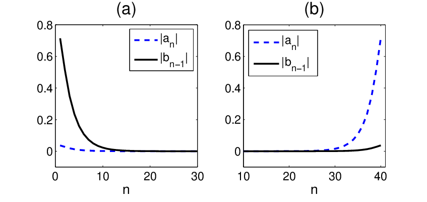
The first case we consider is that of isotropic waveguides rotating in phase with each other (28) [see Fig. 3(a)]. We find this case supports unidirectional edge states. Typical eigenfunctions from both curve branches are displayed in Fig. 4. The eigenmode shown in Fig. 4(a) corresponds to the left zig-zag edge and has strictly negative group velocity i.e. $\alpha^{\prime}(\omega)<0$ . The situation is reversed for edge modes on the right zig-zag edge, shown in Fig. 4(b), that have positive group velocity ( $\alpha^{\prime}(\omega)>0$ ). Taken together, this indicates that the edges modes on a finite domain propagate along the boundary of the lattice in a counter-clockwise fashion, the same direction of the rotating waveguides. Moreover, the outer boundary modes [ $|b_{0}|$ in Fig. 4(a)] are found to have approximately 20 times larger magnitude than the inner boundary mode [ $|a_{1}|$ in Fig. 4(a)].

An asymptotic theory, given in Appendix C, yields (to leading order) left zig-zag edge modes

a_{mn}(z;\omega_{0})=0\;,~~b_{mn}(z;\omega_{0})=C(z)b_{n}^{s}(\omega_{0})e^{im\omega_{0}}\;,

(33)

evaluated at the wavemode $\omega_{0},$ where $C(z)=C_{0}\exp{\left(-i\epsilon\tilde{\alpha}z\right)}$ for constant $C_{0}$ and $\tilde{\alpha}(\omega_{0})$ is found explicitly in terms of integrals; it is given in Eq. (65). The theory is valid in the regime where the waveguides are rapidly oscillating ( $|\epsilon|\ll 1$ ) and describes edge modes in the central gap near $\alpha=0$ ; we refer to this gap as the Floquet center. Where applicable, the asymptotic solutions are compared against those computed numerically.

Next we consider when the waveguides are rotating in phase with each other (28) but are anisotropic ( $\sigma_{x}\not=\sigma_{y}$ ). The band structure in Fig. 3(b) has lost its topologically protected edge character and we expect backscatter. This observation comes from the fact that the slope of edge curves are no longer sign-definite in one Brillouin zone. We point out that this structure only occurs when $\sigma_{x}>\sigma_{y}$ i.e. when the waveguides are elliptical with the major axis in the $x$ -direction (also $n$ -direction). In terms of the results presented in [23], this regime corresponds to $\rho<1/2.$

We now examine when the two sublattices have the same phase, but one of the waveguides has a radius that is three-quarters or half the size of the other (29) : Fig. 3(c-d). In the first case ( $R_{a}=3/4$ ), the crossing modes observed in Fig. 3(a) have deformed into the non-crossing curves seen in Fig 3(c), which still have a sign-definite slope. The fundamental Floquet exponent, $\tau=0$ , as well as the first non-fundamental Floquet bands, $\tau=\pm 1$ , defined in Eq. (27) are shown in Fig. 3(d). The point at which these two branches meet is $\alpha=\pm\pi/T$ . We refer to this point as the Floquet edge. We see that there is a family of edge modes that live in this Floquet edge gap; and the modes in this gap are unidirectional.

Now let us consider a $\pi-$ phase offset between the two sublattices (30). The band structure for this arrangement is shown in Figs. 3(e-f). Included is the fundamental Floquet band ( $\tau=0$ ) as well as its periodic extensions, $\tau=\pm 1.$ Presentation of the different branches of the Floquet bands in Fig. 5 illustrates how one can understand the meeting/merging of the the inter-band curves near the Floquet edge. At sufficiantly small helix radii the band structure consists of bulk bands separated by gaps and exhibits no edge modes. As the radius of the lattice helix, measured by $\eta$ , increases the gap between the adjacent Floquet bands begins to close until the bands “kiss” each other at a single point in Fig. 3(e). This point marks a transition from which any additional driving introduces a new family of topologically protected edge modes at the Floquet edge [see Fig. 3(f)]. We point out that these edge states are distinct from those at the Floquet center. Another feature that we observe in this case, unlike the case in Fig. 3(a), is that the edge states do not remain as $\epsilon\rightarrow 0$ (This is shown in Fig. 11).

The next case examined is that of counter rotation (31). The bands corresponding to this case are shown in Fig. 3(g). We find two flat bands, separated by a small gap, that correspond to non-traveling states. The opposing motion of the two sublattices evidently cancel each other out yielding zero net movement; i.e. essentially a stationary state. The final scenario is when one sublattice has twice the frequency of the other sublattice (29). The band structure, displayed in Fig. 3(h), exhibits a set of topologically protected edge modes. We find that this configuration may possess a weak instability[, namely, $|{\rm Im}~\alpha|=\mathcal{O}(10^{-3})$ ; i.e. it would be a weak exponentially growing/decaying mode that would only manifest itself after a long distance.

III.2 Linear edge mode dynamics in honeycomb lattice

In this section we explore the dynamics of the linear edge states found in Fig. 3. Specifically, we numerically integrate the full tight-binding system (17)-(18) corresponding to solutions of the form given in Eq. (33). In all simulations we omit nonlinearity: $\sigma=0.$ The solutions are initialized at a chosen frequency, $\omega_{0},$ by

a_{mn}(0)=0\;,~~~~~~b_{mn}(0)={\rm sech}\left(\mu m\right)b_{n}(\omega_{0})e^{im\omega_{0}}\;,

(34)

where $\mu=0.3$ denotes the slowly varying envelope and $b_{n}(\omega_{0})$ is the numerically computed mode whose Floquet bands are shown in Fig. 3. For consistency, we normalize all edge modes so the two-norm is one, namely $<b_{n},b_{n}>=1$ via the discrete inner product $<f_{n},g_{n}>=\sum_{n}f_{n}^{*}g_{n}.$ We take periodic boundary conditions in the $m$ -direction and zero boundary conditions in the $n$ -direction. For all $z$ -evolutions shown in this paper we take $N=100$ sites in the $n$ -direction to ensure the mode has sufficiently decayed. The system is integrated using a fourth-order Runge-Kutta method.

Several typical evolutions are displayed in Fig. 6. In the left column we show the solution magnitude at the left boundary of the domain i.e. $n=0$ . In the right column the maximum magnitude for both $a_{mn}(z)$ (in blue) and $b_{mn}(z)$ (in black) over the entire domain are given. In Figs. 6(a-b) the propagation of a topologically protected edge mode, whose dispersion curves are given in Fig. 3(a), is shown. The traveling mode moves in the negative direction at a constant speed. At a point of inflection, $\alpha^{\prime\prime}(\omega)=0$ , a method of stationary phase calculation shows that the edge mode decays like $\sim z^{-1/3}$ . Next in Figs. 6(c-d) a stationary edge state that is not topologically protected [corresponding to the bands in Fig. 3(b)] is shown. In contrast to the previous case, this state is diffracting and losing amplitude at a rapid pace. Asymptotically, when $\alpha^{\prime\prime}(\omega)\not=0$ the mode decays like $\sim z^{-1/2}$ .

The next mode we consider is located near the Floquet edge in Fig. 3(f) and corresponds to $\pi$ -offset rotation. Unlike the previous two cases, whose energy is always in the $b_{m0}$ lattice sites, this solution [shown in Figs. 6(e-f)] is observed to oscillate back-and-forth between the $b_{m0}$ and $a_{m1}$ lattice sites. Energy is regularly transferred back-and-forth each cycle of the lattice waveguides (here the period is $T=1.5$ ). A similar evolution pattern (not shown here) was found to occur for the edge state mode corresponding to different sublattice radii whose Floquet bands are shown in Fig. 3(d).

Floquet theory does tell us something about this coupled-mode dynamic. Typically, the 1D honeycomb Eqs. (20)-(21) are integrated over the period $[0,T]$ to find the fundamental matrix solution. The corresponding edge mode eigenfunction [similar to that in Fig. 4(a)] has considerably more energy in the outer $b_{n}$ sites than those of $a_{n}$ . If we instead calculate the Floquet multipliers over the interval $[T/2,3T/2]$ , then the energy is primarily concentrated in the $a_{n}$ sites, rather than $b_{n}$ . From this observation we infer that these solutions are not of the form given in Eq. (33), and instead resemble $a_{n}(z)=A(z)r^{n}$ and $b_{n}(z)=B(z)r^{n}$ for $|r|<1,n=0,1,2,\dots$ , where $A(z)$ and $B(z)$ are $T$ -periodic envelopes. In other words, the modes are truly coupled ( $a_{n}\not=0$ ) and can not be assumed to be scalar ( $a_{n}\approx 0$ ).

III.3 Staggered square Floquet bands

In this section the Floquet bands for the staggered square lattice in Fig. 2 are computed for the rotation patterns described earlier in equations (28)-(32). The Floquet exponent (27) is computed from 1D staggered square system (25)-(26). Several band structures are shown in Fig. 7.

The first lattice configuration we examine is when the two sublattices rotate in phase with each other given in equation (28). In this case, the system given in Eqs. (25)-(26) is degenerate and reduces to a single equation. In terms of the lattice structure, the lattice sites form a simple lattice. There are no edge modes at all, as indicated in Fig. 7(a); there are only extended bulk modes. One way to create a non-simple lattice configuration is to make the radius of one sublattice smaller than the other. The dispersion bands for this scenario are shown in Figs. 7(c) and 7(d) where the radii of one sublattice is $75\%$ and $60\%$ , respectively, the size of the other. As the radius disparity grows, localized edge state curves manifest themselves in the gap at the Floquet edge. This latter band structure is distinguished from all other cases in that for certain positive $\omega$ values there exist two different Floquet exponents: one topologically-protected near the Floquet edge and the other non-protected near the Floquet center. In most of the topological systems we investigated, either one or the other mode types exist at a fixed $\omega$ , but not both.

The two rotation patterns we consider next are counter rotation (see equation (31) and $\pi$ -phase offset rotation (see equation (30). First, we examine the counter rotation case whose Floquet bands are shown in Fig. 7(b). If the radius of the sublattices are driven hard enough, then, similar to the honeycomb case, the bulk band splits apart and inside the central gap an edge mode corresponding to a nearly flat band is found to exist. Next we consider a $\pi$ -offset rotation. We point out that this scenario was explored in [19, 20]. Qualitatively, our results agree with theirs, namely there is a transition point in the topological structure of the bands that is displayed in Fig. 7(e). Below this transition point, in a weak rotation regime, the band structure takes a “trivial” form similar to that seen in Fig. 7(a). If, on the other hand, the spiral radius is increased beyond this threshold a set of topologically protected edge modes emerge and give the “nontrivial” band structure shown in Fig. 7(f). This transition point in band structure resembles the honeycomb cases given in Figs. 3(e-f).

The final case we consider is that of different frequency between the two sublattices (see equation (32). For a large enough helix radius, edge states are found to occur near the Floquet edge. Similar to the honeycomb case in Fig. 3(h), these states appear to possess a weak instability [ $|{\rm Im}~\alpha|=\mathcal{O}(10^{-3})$ ] that could become relevant over very long propagation distances.

At this point we summarize the commonalities in the linear band structures between the honeycomb and staggered square lattices. In the case of same rotation patterns we find that edge modes are present if the underlying lattice is fundamentally non-simple (like honeycomb, or staggered with different sublattice size or frequency). Taking sufficiently different radii among the sublattices creates edge states at the Floquet edges, for both lattice types. Stationary (or nearly stationary) edge modes are generated in the case of counter-rotating sublattices. A family of edge modes is found to exist between different branches of Floquet bands (27) for $\pi$ -offset rotation when the waveguide parameters exceed a certain threshold. When the two sublattices have different frequencies edge modes can be found (with a possible weak instability).

III.4 Linear edge mode dynamics in staggered square lattice

In this section we propagate the linear modes associated with the dispersion curves shown in Fig. 7. The governing equations (22)-(23) are integrated using initial conditions of the form

a_{2m+1,2n+1}(0)=0\;,~~b_{2m,2n}(0)={\rm sech}\left(2m\mu\right)b_{2n}(\omega_{0})e^{i2m\omega_{0}}\;,

(35)

where $\mu=0.3$ and the decaying mode $b_{2n}$ is numerically computed from the 1D system (25)-(26). As was the case in honeycomb lattice, we take $N=100$ lattice sites in the $n$ -direction for both $b_{2m,2n}$ and $a_{2m+1,2n+1}$ . For all cases considered here we display the edge magnitude as well as the maximum magnitude over the domain as a function of $z$ .

The first nontrivial case we consider is that of counter-rotation whose corresponding dispersion curves are shown in Fig. 7(b). The Floquet bands are nearly flat and so very little translation of the localized mode is expected. The edge mode evolution is shown in Figs. 8(a-b) and indeed the mode is well-localized, has a small positive velocity and most of the energy is in the ‘ $b$ ’ mode. Next we look at the case of different radii among the sublattices corresponding to the bands displayed in Fig. 7(d). The edge wave propagation and magnitude evolution is shown in Figs. 8(c-d). Similar to the honeycomb dynamics above, the edge modes whose Floquet exponents reside in the Floquet edge gap are observed to pivot back-and-forth among the $b_{2m,0}$ and $a_{2m+1,1}$ lattice sites. The energy is observed to oscillate with the same frequency as the lattice, $T=1.5$ . There is an additional submode excited in Fig. 8(c) that is moving left-to-right and corresponds to the mode located near $\alpha(\pi/10)\approx 4$ in Fig. 7(d). Moreover, this right moving mode is not a protected solution i.e. it will scatter at defects. It was numerically verified that the left-moving mode interacted with a defect like the topologically protected mode shown in the top row of Fig. 12; i.e. this mode travelled through the defect. On the other hand, the right-traveling mode was found to scatter off a defect like the mode displayed in the bottom row of Fig. 12. For the cases we studied it was unusual to have a system that simultaneously supports both topological and non-topological edge states.

In Figs. 8(e-f) which corresponds to Fig. 7(f) the $\pi$ -offset edge profile is found to oscillate back-and-forth between the $a$ and $b$ sites with the same period as that of the helix ( $T=1.5$ ). This dynamics pattern resembles the $\pi$ -offset honeycomb evolution shown in Fig. 6(e-f). Between the honeycomb and square evolutions we can see that similar lattice rotation patterns often yield similar edge mode evolutions, when the underlying band structures are similar.

IV Edge Solitons

In this section we explore the nonlinear ( $\sigma\not=0$ ) equations given in Sec. II. Using an asymptotic analysis, valid in the small $\epsilon$ regime, we find true edge soliton solutions, i.e. edge modes modulated by a slowly-varying envelope function that satisfies the NLS equation. Direct numerical simulations are used to validate our asymptotic results. On the other hand, this asymptotic theory does not describe every possible edge mode found in Sec. III. As we have remarked, modes located and the Floquet edge can disappear as $\epsilon\rightarrow 0,$ and therefore are outside the scope of our small $\epsilon$ analysis.

To leading order, we find 2D zig-zag edge mode solutions to Eq. (17)-(18) of the form

a_{mn}(z)=0\;,~~~b_{mn}(z)=C(y,z)b_{n}(\omega_{0})e^{im\omega_{0}}\;,

(36)

where the envelope function, $C(y,z)$ , satisfies the NLS-type equation

	$\displaystyle i\frac{\partial C}{\partial z}$	$\displaystyle-\alpha_{0}C+i\alpha_{0}^{\prime}C_{y}+\frac{\alpha_{0}^{\prime\prime}}{2}C_{yy}-i\frac{\alpha_{0}^{\prime\prime\prime}}{6}C_{yyy}+\dots$
		$\displaystyle+\alpha_{\rm nl}(\omega_{0})\|C\|^{2}C+\dots=0\;,$		(37)

such that $\tilde{\alpha}_{0}^{(j)}=\frac{d^{j}\tilde{\alpha}}{d\omega^{j}}\big|_{\omega=\omega_{0}}$ and the function $C(y,z)$ varies slowly in $y$ , i.e. $|\partial_{y}C|\ll 1$ . The variable $y$ is slowly-varying in the $m$ -direction. The details of the analysis are given in Appendix C. In the direction perpendicular to the zig-zag edge, the solution in (36) decays like the stationary mode $b_{n}^{s}=r^{n}$ for $|r|<1$ [the value of $r(\omega_{0})$ is defined in Eq. (61)]. This solution is derived under a narrow-band approximation, which assumes that only the frequencies, $\omega$ , near $\omega_{0}$ make substantial contributions to the solution. Then by setting $C(y,Z)=\tilde{C}(y,Z)e^{-i\alpha_{0}Z}$ we obtain (to leading order) the NLS equation

i\frac{\partial\tilde{C}}{\partial z}+i\alpha_{0}^{\prime}C_{y}+\frac{\alpha_{0}^{\prime\prime}}{2}\tilde{C}_{yy}+\alpha_{\rm nl}(\omega_{0})|\tilde{C}|^{2}\tilde{C}=0\;,

(38)

which for $\alpha_{0}^{\prime\prime}>0$ (focusing) has the traveling soliton solution

\tilde{C}(y,z)=\mu\sqrt{\frac{\alpha_{0}^{\prime\prime}}{\alpha_{\rm nl}}}{\rm sech}\left[\mu(y-\alpha_{0}^{\prime}z)\right]e^{i\frac{\mu^{2}\alpha_{0}^{\prime\prime}}{2}z}\;,

(39)

with $\mu\geq 0$ . At points of inflection [like at $\omega=\pi/2$ in Fig. 3(a)], $\alpha_{0}^{\prime\prime}=0$ and therefore the leading order dispersive term is now third-order and we get the higher-order NLS equation

i\frac{\partial\tilde{C}}{\partial Z}+i\alpha_{0}^{\prime}C_{y}-i\frac{\alpha_{0}^{\prime\prime\prime}}{6}\tilde{C}_{yyy}+\alpha_{\rm nl}(\omega_{0})|\tilde{C}|^{2}\tilde{C}=0\;,

(40)

which does not support solitons.

Next, we numerically verify these asymptotic results by direct numerical simulations performed on the full tight-binding system (17)-(18). Here we restrict our attention to the nonlinear modes found using our asymptotic theory (corresponding to red curves in Fig. 3). Analysis of the remaining modes is outside the scope of this paper.

To initialize the simulations we take functions of the form in Eq. (36). For the figures shown here the linear decaying mode, $b_{n}^{s}$ , were computed numerically, but we did check that the asymptotic solution, $b_{n}^{s}=r^{n}$ , gave similar results. We normalize the edge mode two-norm so that $<b_{n},b_{n}>=1.$ The envelope is initialized by the localized function

C(y=\mu m,z)=A~{\rm sech}\left(\mu m\right)\;,~~~A\geq 0\;,

(41)

for an amplitude, $A$ , chosen to balance the leading-order dispersion term (either $\alpha_{0}^{\prime\prime}\mu^{2}$ or $\alpha_{0}^{\prime\prime\prime}\mu^{3}$ ) with the cubic nonlinearity, $A^{2}\alpha_{\rm nl}.$

Two edge mode evolutions are displayed in Fig. 9. In the first case, a traveling mode whose corresponding linear edge mode [located at $\omega_{0}=\pi/2$ in Fig. 3(a)] is at a point of inflection ( $\alpha_{0}^{\prime\prime}=0$ ). This implies that the envelope is governed by the higher-order NLS Eq. (40) which does not support pure soliton modes. A closer comparison of the full discrete solution on the domain boundary, $b_{m0}$ , and the envelope $C(y,z)$ is shown in Fig. 10, where the initial and final solution profiles are shown in Figs. 10(a) and 10(b), respectively. The envelope captures the translation and a small dispersive tail which becomes more pronounced as $z$ grows.

The next case we consider is when the envelope function satisfies the classic NLS equation (38). We choose the same lattice parameters that correspond to the linear Floquet bands shown in Fig. 3(b). At the point $\omega_{0}=3\pi/4$ the value of $\alpha_{0}^{\prime\prime}$ is positive indicating that the NLS equation (38) is focusing and thus admits soliton modes. The evolution of such a nonlinear edge mode is shown in Fig. 9(b). The mode is stationary because $\alpha_{0}^{\prime}=0$ . A closer look at the initial and final edge soliton profiles is given in Figs. 10(c-d). Comparing these two figures we see that the final magnitude is nearly the same as that which was initially injected. In both this case and previous one there is a small gap between the envelope and discrete mode peaks that may be attributed to some energy being transferred from the $b_{mn}$ mode into the $a_{mn}$ mode. We also remark that in the latter case it so happens that $|b_{0}|<1$ , so there is also an initial gap at $z=0.$

The asymptotic results shown here only cover edge modes located near the Floquet center. Moreover, the curves at the Floquet edges in Figs. 3 and 7 are the result of finite $\epsilon$ and disappear as $\epsilon\rightarrow 0.$ This is highlighted in Fig. 11. In this case there are two distinct families of edge modes: one that bifurcates from the stationary mode [located near $\alpha=0$ in Fig. 11(a)] and another [located near $\alpha=\pm\pi/T$ in Fig. 11(a)] separate one that arises when the helix period is not necessarily small in comparison to the characteristic propagation distance scale (not oscillating too fast). As $\epsilon$ approaches zero the edge modes at the Floquet edge are observed to disappear, leaving only those modes predicted by the asymptotic theory in Appendix C. Indeed, to understand a mode that oscillates like the linear edge state in Fig. 6(e) requires a true coupled-mode theory, i.e. not setting $a_{mn}=0$ , to account for this back-and-forth energy transfer. To understand this finite $\epsilon$ edge modes is beyond the scope of this paper.

V Lattice Defects

Lattice defects and imperfections are common in any real photonic lattice. Here we consider a scenario where many lattice sites are absent along the boundary, thereby introducing a boundary notch, or wall. The absence of any lattice sites along the boundary means the wave field is effectively zero there. To implement these boundary effects into the tight-binding model above we set $a_{mn}=b_{mn}=0$ at the lattice defect locations. To track the evolution dynamics of the edge mode as it confronts the defect two quantities are monitored: the maximum intensities, $|a_{mn}(z)|^{2}$ and $|b_{mn}(z)|^{2}$ , and the ‘participation’ ratio

P_{b}(z)=\frac{\left(\sum_{m,n}|b_{mn}|^{2}\right)^{2}}{\sum_{m,n}|b_{mn}|^{4}}\;.

(42)

The first quantity measures the edge mode peaks, while the latter gives a measure of the pulse width since (42) is proportional to it.

We focus our attention on three illuminating examples. In the first situation we evolve a linear ( $\sigma=0$ ) topologically protected edge mode whose corresponding Floquet exponent is given in Fig. 3(a) at $\omega_{0}=\pi/2.$ The evolution of the edge mode when it comes into contact with the lattice defect is shown in Fig. 12. In most non-topological systems significant scattering would be expected. Here, however, the edge mode tracks around the boundary notch and exhibits no backscattering. The intensity and participation ratio evolutions in Fig. 13 shed some light on the edge mode-defect dynamics. Along the defect boundaries perpendicular to the $n=0$ axis the boundaries have armchair configurations. It is here that the energy begins to evenly distribute between the modes [see Fig. 13(a)]. In addition, the outer edge mode, $b_{m0}$ , is found to spread to many sites (become wider) [see Fig. 13(b)] along these armchair boundaries. The outgoing intensity is observed to have nearly the same magnitude as the incoming value.

The second case we consider is that of a non-topologically protected mode. The corresponding Floquet exponent is shown in Fig. 3(b) at $\omega_{0}=\pi/2.$ Recall that this mode resulted from elongating the waveguide geometries in the direction perpendicular to the zig-zag boundary. The edge mode dynamics shown in Fig. 12 contrast from those in the previous case. Upon making contact with the defect boundary the edge mode scatters back in the opposite direction. From Fig. 13(c) the mode intensity is found to double at the defect corner, meanwhile Fig. 13(d) shows that the pulse width is cut in half (becomes more localized). Upon reflecting backwards significant dispersion in the edge state is observed.

Finally, we consider the interaction of a nonlinear edge mode with a defect. In particular, we focus on states we refer to as topologically protected edge solitons. These modes are characterized by linear Floquet bands with sign-invariant group velocity [see Fig. 3(a)] whose envelopes, to leading order, satisfy the NLS equation (38). In general, we expect these states to combine the robustness of solitons with the unidirectionality of a protected state. Consider dispersion bands like those shown in Fig. 3(a). At the point $\omega=5\pi/8\approx 1.963$ we have $\alpha_{0}^{\prime\prime}>0$ and $|\alpha_{0}^{\prime\prime\prime}|\ll 1$ , yet $\alpha_{0}^{\prime}<0.$ In this case the traveling envelope satisfies the focusing NLS equation and therefore it is a true soliton. One such case is displayed in Fig. 14. This nonlinear edge mode is observed to track around the defect just like the linear protected mode in Fig. 12. The outgoing soliton intensity is found to be nearly the same as the incoming magnitude. The maximum intensity and the participation ratio for this case are shown in Fig. 15. These values closely resemble the linear ones in Figs. 13 (a-b). One difference is that some loss is in the magnitude is observed in nonlinear case. This may be attributed to the fact that we are not in the pure NLS (38), but instead of a small amount of higher-order dispersion, since $\alpha_{0}^{\prime\prime\prime}\not=0$ . This extra dispersion results in a small amount of radiation being emitted from the mode Decreasing the value of $\mu$ should improve the asymptotic NLS approximation.

VI Conclusions

We have introduced a direct method for deriving tight-binding approximations of beam propagation in general 2D longitudinally driven waveguide arrays. As prototypes we examined periodically driven honeycomb and staggered square lattices. The new set of governing equations we derived allows us to find and examine unexplored edge modes with rather complicated sublattice rotation patterns such as: counter rotation, different radii, different frequency, different structure and $\pi$ -phase offset. We computed the linear Floquet bands for these rotation configurations and also examined their evolutions.

An asymptotic theory was developed; it showed that the nonlinear edge modes behave as linear edge states modulated by a slowly-varying envelope that satisfies the 1D nonlinear Schrödinger equation. Ideal nonlinear edge modes combine the scatter-free topological properties of the linear problem with the robust nature of solitons.

Finally, topologically protected modes, both linear and nonlinear, were shown to possess unidirectionality (absence of backscatter), even when encountering strong lattice defects. In the absence of topological protection the mode simply reflects off a barrier. The approach for deriving tight-binding equations and analyzing photonic topological insulators allows the exploration of many new Floquet and non-Floquet lattice systems.

Appendix A Additional Tight-binding Details

Here we provide some additional comments/details on deriving the honeycomb lattice tight-binding approximation in Sec. II. The derivation for the staggered square lattice follows in a similar manner. The ansatz in Eq. (11) is defined in terms of the two Gaussian orbital functions $\widehat{\phi}_{1,{\bf v}}({\bf r},z)$ and $\widehat{\phi}_{2,{\bf v}}({\bf r},z)$ centered at the points ${\bf v}$ and ${\bf v}+{\bf d}+\Delta{\bf h}_{12}(z)$ , respectively. These evanescent functions are taken to satisfy a linear ( $\sigma=0$ ) and local ( ${\bf r}\rightarrow{\bf r}_{j},{\bf r}_{k}$ ) set of weakly-rotating ( $|{\bf A}_{z}|\ll 1$ ) equations

		$\displaystyle i\frac{\partial\widehat{\phi}_{1,{\bf v}}}{\partial z}+\nabla^{2}\widehat{\phi}_{1,{\bf v}}-V_{\rm loc}({\bf r}-{\bf{v}})=0\;,$		(43)
		$\displaystyle i\frac{\partial\widehat{\phi}_{2,{\bf v}}}{\partial z}+\nabla^{2}\widehat{\phi}_{2,{\bf v}}-V_{\rm loc}({\bf r}-({\bf{d}}+{\bf{v}})-\Delta{\bf h}_{21}(z))=0\;,$		(44)

where

V_{\rm loc}({\bf r})=V_{0}^{2}\left(\frac{x^{2}}{\sigma_{x}^{2}}+\frac{y^{2}}{\sigma_{y}^{2}}\right)\;.

(45)

In particular, the normalized orbital functions used are

		$\displaystyle\widehat{\phi}_{1,{\bf v}}({\bf r},z)=\phi_{1,{\bf v}}({\bf r})e^{-iEz}\;,$		(46)
		$\displaystyle\widehat{\phi}_{2,{\bf v}}({\bf r},z)=\phi_{2,{\bf v}}({\bf r},z)e^{-iEz}\;,$		(47)

where $\phi_{1,{\bf v}}({\bf r})=\phi({\bf r}-{\bf v})$ and $\phi_{2,{\bf v}}({\bf r},z)=\phi({\bf r}-({\bf d}+{\bf v})-\Delta{\bf h}_{21}(z))$ for

\phi({\bf r})=\sqrt{\frac{V_{0}}{\pi\sqrt{\sigma_{x}\sigma_{y}}}}e^{-\frac{V_{0}}{2}\left[\frac{x^{2}}{\sigma_{x}}+\frac{y^{2}}{\sigma_{y}}\right]}\;,~~E=V_{0}\left(\frac{1}{\sigma_{x}}+\frac{1}{\sigma_{y}}\right)\;.

(48)

Substituting ansatz (11) into Eq. (9) for the Gaussian orbitals that satisfy Eqs. (43)-(44) yields

		$\displaystyle\sum_{\bf v}\bigg[\bigg(i\frac{da_{\bf v}}{dz}\phi_{1,{\bf v}}+i\frac{db_{\bf v}}{dz}\phi_{2,{\bf v}}\bigg)$		(49)
		$\displaystyle+iV_{0}\frac{(\Delta{\bf h}^{\prime}_{21}(z))_{x}[{\bf r}-({\bf v}+{\bf d})-\Delta{\bf h}_{21}(z)]_{x}}{\sigma_{x}}b_{\bf v}\phi_{2,{\bf v}}$
		$\displaystyle+iV_{0}\frac{(\Delta{\bf h}^{\prime}_{21}(z))_{y}[{\bf r}-({\bf v}+{\bf d})-\Delta{\bf h}_{21}(z)]_{y}}{\sigma_{y}}b_{\bf v}\phi_{2,{\bf v}}$
		$\displaystyle+{\bf r}\cdot{\bf A}_{z}\big[a_{\bf v}\phi_{1,{\bf v}}+b_{\bf v}\phi_{2,{\bf v}}\big]$
		$\displaystyle-a_{\bf v}\phi_{1,{\bf v}}\left[V({\bf r},z)-V_{\rm loc}({\bf r}-{\bf v})\right]$
		$\displaystyle-b_{\bf v}\phi_{2,{\bf v}}\left[V({\bf r},z)-V_{\rm loc}({\bf r}-({\bf v}+{\bf d})-\Delta{\bf h}_{21}(z))\right]\bigg]e^{ik\cdot{\bf v}}$
		$\displaystyle=0\;,$

where subscripts $x$ and $y$ denote the $\hat{\imath}$ and $\hat{\jmath}$ vector components, respectively. We next multiply this equation by $\phi_{1,{\bf p}}({\bf r})$ and $\phi_{2,{\bf p}}({\bf r},z)$ and integrate to get the ‘a’ and ‘b’ mode equations given in Eqs. (17) and (18), respectively. For deep lattices ( $V_{0}\gg 1$ ) we may consider only the self and nearest-neighbor interactions to good approximation.

Following integration of the orbital functions, several simplifications to the remaining equations can be made. All self-interaction phase terms can be removed by the simple transformation $a_{{\bf p}+{\bf v}}(z)=\tilde{a}_{{\bf p}+{\bf v}}(z)\exp(i\Phi_{{\bf p}+{\bf v}}(z))$ and $b_{{\bf p}+{\bf v}}(z)=\tilde{b}_{{\bf p}+{\bf v}}(z)\exp(i\Theta_{{\bf p}+{\bf v}}(z))$ where

	$\displaystyle\Phi_{{\bf p}+{\bf v}}(z)=({\bf p}+{\bf v})\cdot{\bf A}(z)-z\bigg[V_{0}^{2}-\frac{V_{0}}{2}\left(\frac{1}{\sigma_{x}}+\frac{1}{\sigma_{y}}\right)$
	$\displaystyle~~~~~~~~~~~~~~~~~~~~~~~~~~~~~-V_{0}^{3}\sqrt{\frac{\sigma_{x}\sigma_{y}}{(1+\sigma_{x}V_{0})(1+\sigma_{y}V_{0})}}\bigg]\;,$	(50)
	$\displaystyle\Theta_{{\bf p}+{\bf v}}(z)=({\bf p}+{\bf d}+{\bf v})\cdot{\bf A}(z)+\int_{0}^{z}\Delta{\bf h}_{21}(\zeta)\cdot{\bf A}_{\zeta}(\zeta)d\zeta$
$\displaystyle-$	$\displaystyle z\bigg[V_{0}^{2}-\frac{V_{0}}{2}\left(\frac{1}{\sigma_{x}}+\frac{1}{\sigma_{y}}\right)-V_{0}^{3}\sqrt{\frac{\sigma_{x}\sigma_{y}}{(1+\sigma_{x}V_{0})(1+\sigma_{y}V_{0})}}\bigg]\;.$	(51)

Next it is observed that $\left|da_{\bf p}/dz\right|=\left|db_{\bf p}/dz\right|=\mathcal{O}\left(\exp[{-V_{0}|{\bf d}|^{2}/(4\sigma)}]\right)$ . Since the off-diagonal derivative terms are of the form $\exp[{-V_{0}|{\bf d}|^{2}/(4\sigma)}]da_{\bf p}/dz$ they are exponentially smaller than all other terms and may be neglected. We only consider the remaining dominant terms. These terms are numerically identified to be those with a coefficients of $V_{0}$ or $V_{0}^{2}$ (since we are in the deep lattice limit) and all other terms are dropped. Finally, to simplify working with these equations we relabel our grid in terms of a two-dimensional square lattice indexed as in Fig. 1.

Appendix B Tight-binding Approximation Coefficients

In this section the tight-binding approximation coefficients for the honeycomb lattice given in Eqs. (17)-(18), and the staggered square lattice (22)-(23). The subscripts $x$ and $y$ denote the $\hat{\imath}$ and $\hat{\jmath}$ vector components, respectively. The nonlinearity coefficient in both cases is given by

\sigma=\frac{\gamma V_{0}}{2\pi\sqrt{\sigma_{x}\sigma_{y}}}\;.

(52)

B.1 Honeycomb Lattice

The terms composing the honeycomb linear operator defined below Eqs. (17)-(18) are

	$\displaystyle\mathbb{L}_{j}(z)=$	$\displaystyle V_{0}^{3}\sqrt{\frac{\sigma_{x}\sigma_{y}}{(1+\sigma_{x}V_{0})(1+\sigma_{y}V_{0})}}$
		$\displaystyle\times\bigg\{2e^{-\frac{V_{0}}{4}\left[\frac{[{\bf d}-{\bf v}_{j}+\Delta{\bf h}_{21}(z)]_{x}^{2}}{\sigma_{x}(1+V_{0}\sigma_{x})}+\frac{[{\bf d}-{\bf v}_{j}+\Delta{\bf h}_{21}(z)]_{y}^{2}}{\sigma_{y}(1+V_{0}\sigma_{y})}\right]}-1\bigg\}$
	$\displaystyle+\frac{V_{0}^{2}}{4}$	$\displaystyle\left\{\frac{[{\bf d}-{\bf v}_{j}+\Delta{\bf h}_{21}(z)]^{2}_{x}}{\sigma_{x}^{2}}+\frac{[{\bf d}-{\bf v}_{j}+\Delta{\bf h}_{21}(z)]^{2}_{y}}{\sigma_{y}^{2}}\right\}\;,$

	$\displaystyle\mathbb{R}_{j}(z)$	$\displaystyle=\frac{V_{0}}{2}\bigg[\frac{\left[\Delta{\bf h}_{21}^{\prime}(z)\cdot({\bf d}-{\bf v}_{j}+\Delta{\bf h}_{21}(z))\right]_{x}}{\sigma_{x}}+$
		$\displaystyle~~~~~~~~~~~~+\frac{\left[\Delta{\bf h}_{21}^{\prime}(z)\cdot({\bf d}-{\bf v}_{j}+\Delta{\bf h}_{21}(z))\right]_{y}}{\sigma_{y}}\bigg]\;,$

and

c_{j}(z)=e^{-\frac{V_{0}}{4}\left[\frac{[{\bf d}-{\bf v}_{j}+\Delta{\bf h}_{21}(z)]_{x}^{2}}{\sigma_{x}}+\frac{[{\bf d}-{\bf v}_{j}+\Delta{\bf h}_{21}(z)]_{y}^{2}}{\sigma_{y}}\right]}\;,

where $\Delta{\bf h}_{21}(z)={\bf h}_{2}(z)-{\bf h}_{1}(z),$ and the vectors ${\bf d}=(1,0),{\bf v}_{0}={\bf 0},{\bf v}_{1}=(3,\sqrt{3})/2$ and ${\bf v}_{2}=(3,-\sqrt{3})/2$ .

In the special case of same rotation, same phase the following occur: $\Delta{\bf h}_{21}(z)=0,\mathbb{R}_{j}(z)=0,$ and the functions $c_{j}(z)$ and $\mathbb{L}_{j}(z)$ are constant for each $j$ . Rescaling Eqs. (17)-(18) by $Z=c_{0}\mathbb{L}_{0}z$ gives the system considered in [23], namely

		$\displaystyle i\frac{da_{mn}}{dZ}+e^{i{\bf d}\cdot{\bf A}(Z)}\left(\mathcal{L}_{-}(Z)b\right)_{mn}+\sigma\|a_{mn}\|^{2}a_{mn}=0\;,$		(53)
		$\displaystyle i\frac{db_{mn}}{dZ}+e^{-i{\bf d}\cdot{\bf A}(Z)}\left(\mathcal{L}_{+}(Z)a\right)_{mn}+\sigma\|b_{mn}\|^{2}b_{mn}=0\;,$		(54)

where

	$\displaystyle\left(\mathcal{L}_{-}(Z)b\right)_{mn}$	$\displaystyle=b_{mn}$
	$\displaystyle+$	$\displaystyle\rho\left[b_{m-1,n-1}e^{-i\theta_{1}(Z)}+b_{m+1,n-1}e^{-i\theta_{2}(Z)}\right]\;,$

	$\displaystyle\left(\mathcal{L}_{+}(Z)a\right)_{mn}$	$\displaystyle=a_{mn}$
	$\displaystyle+$	$\displaystyle\rho\left[a_{m+1,n+1}e^{i\theta_{1}(Z)}+a_{m-1,n+1}e^{i\theta_{2}(Z)}\right]\;,$

for the geometric parameter

\rho=\frac{c_{1}\mathbb{L}_{1}}{c_{0}\mathbb{L}_{0}}=\frac{c_{2}\mathbb{L}_{2}}{c_{0}\mathbb{L}_{0}}\;.

(55)

The anisotropic Floquet bands considered in Fig. 3(b) correspond to $\rho<1/2$ .

B.2 Staggered Square Lattice

Here we give the definitions for the linear terms defined below Eqs. (22)-(23) are

	$\displaystyle\mathbb{L}_{j}(z)=$	$\displaystyle V_{0}^{3}\sqrt{\frac{\sigma_{x}\sigma_{y}}{(1+\sigma_{x}V_{0})(1+\sigma_{y}V_{0})}}$
		$\displaystyle~~~~~~\times\bigg\{2e^{-\frac{V_{0}}{4}\left[\frac{[{\bf v}_{j}+\Delta{\bf h}_{21}(z)]_{x}^{2}}{\sigma_{x}(1+V_{0}\sigma_{x})}+\frac{[{\bf v}_{j}+\Delta{\bf h}_{21}(z)]_{y}^{2}}{\sigma_{y}(1+V_{0}\sigma_{y})}\right]}-1\bigg\}$
		$\displaystyle+\frac{V_{0}^{2}}{4}\left(\frac{[{\bf v}_{j}+\Delta{\bf h}_{21}(z)]^{2}_{x}}{\sigma_{x}^{2}}+\frac{[{\bf v}_{j}+\Delta{\bf h}_{21}(z)]^{2}_{y}}{\sigma_{y}^{2}}\right)\;,$

	$\displaystyle\mathbb{R}_{j}(z)$	$\displaystyle=\frac{V_{0}}{2}\bigg\{\frac{\left[\Delta{\bf h}_{21}^{\prime}(z)\cdot({\bf v}_{j}+\Delta{\bf h}_{21}(z))\right]_{x}}{\sigma_{x}}$
		$\displaystyle~~~~~~~~~~+\frac{\left[\Delta{\bf h}_{21}^{\prime}(z)\cdot({\bf v}_{j}+\Delta{\bf h}_{21}(z))\right]_{y}}{\sigma_{y}}\bigg\}\;,$

c_{j}(z)=e^{-\frac{V_{0}}{4}\left[\frac{[{\bf v}_{j}+\Delta{\bf h}_{21}(z)]_{x}^{2}}{\sigma_{x}}+\frac{[{\bf v}_{j}+\Delta{\bf h}_{21}(z)]_{y}^{2}}{\sigma_{y}}\right]}\;,

for $j=\pm 1,\pm 2$ and $\Delta{\bf h}_{21}(z)={\bf h}_{2}(z)-{\bf h}_{1}(z)$ . Here we adopt the convention ${\bf v}_{-j}\equiv-{\bf v}_{j}$ . The lattice vectors are defined by ${\bf v}_{1}=(1,1)/\sqrt{2}$ and ${\bf v}_{2}=(1,-1)/\sqrt{2}$ .

Appendix C Asymptotic Analysis

Details for deriving asymptotic solution (36) to the honeycomb lattice system (17)-(18) are presented here. This analysis generalizes the calculation performed in [23] to cover the more general non-synchronized rotation patterns discussed in this paper. The periodic functions $\Delta{\bf h}_{21},{\bf\varphi}$ and ${\bf A}$ are all assumed to depend only on the fast variable $\zeta=z/\epsilon$ , where $|\epsilon|\ll 1$ and weak nonlinearity of $\sigma=\epsilon\tilde{\sigma}$ is assumed. To begin, we take functions of the form given in Eq. (19) and then expand

a_{n}=\sum_{j=0}^{\infty}\epsilon^{j}a_{n}^{(j)}(z,\zeta)\;,~~~b_{n}=\sum_{j=0}^{\infty}\epsilon^{j}b_{n}^{(j)}(z,\zeta)\;.

(56)

For convenience, we gather all linear under the definitions $(\tilde{\mathcal{L}}_{-}b)_{n}\equiv e^{i{\bf d}\cdot{\bf A}(\zeta)+i\varphi(\zeta)}\left(\mathcal{L}_{-}(\zeta)b\right)_{n}$ and $(\tilde{\mathcal{L}}_{+}a)_{n}\equiv e^{-i{\bf d}\cdot{\bf A}(\zeta)-i\varphi(\zeta)}\left(\mathcal{L}_{+}(\zeta)a\right)_{n}$ . Substituting expansions (56) into Eqs. (17)-(18) and keeping the leading order terms gives

\mathcal{O}\left(1/\epsilon\right):~~~~i\frac{\partial a_{n}^{(0)}}{\partial\zeta}=0\;,~~~~i\frac{\partial b_{n}^{(0)}}{\partial\zeta}=0\;,

(57)

which implies that $a_{n}^{(0)}(z,\zeta)=a_{n}^{(0)}(z)$ and $b_{n}^{(0)}(z,\zeta)=b_{n}^{(0)}(z)$ . At the next order we get

	$\displaystyle\mathcal{O}(1):~~~~$	$\displaystyle i\frac{\partial a_{n}^{(1)}}{\partial\zeta}=-i\frac{da_{n}^{(0)}}{dz}-(\tilde{\mathcal{L}}_{-}b^{(0)})_{n}\;,$		(58)
		$\displaystyle i\frac{\partial b_{n}^{(1)}}{\partial\zeta}=-i\frac{db_{n}^{(0)}}{dz}-(\tilde{\mathcal{L}}_{+}a^{(0)})_{n}\;.$

To eliminate secularities these equations are rewritten as

		$\displaystyle i\frac{\partial a_{n}^{(1)}}{\partial\zeta}=-\left[(\tilde{\mathcal{L}}_{-}b^{(0)})_{n}-\overline{(\tilde{\mathcal{L}}_{-}b^{(0)})}_{n}\right]-f_{-}\;,$		(59)
		$\displaystyle i\frac{\partial b_{n}^{(1)}}{\partial\zeta}=-\left[(\tilde{\mathcal{L}}_{+}a^{(0)})_{n}-\overline{(\tilde{\mathcal{L}}_{+}a^{(0)})}_{n}\right]-f_{+}\;,$

where

		$\displaystyle f_{-}=i\frac{\partial a_{n}^{(0)}}{\partial z}+\overline{(\tilde{\mathcal{L}}_{-}b^{(0)})}_{n}\;,$		(60)
		$\displaystyle f_{+}=i\frac{\partial b_{n}^{(0)}}{\partial z}+\overline{(\tilde{\mathcal{L}}_{+}a^{(0)})}_{n}\;,$

are zero at this order and we define the average: $\overline{c}=\left(\int_{0}^{T}c(\zeta)d\zeta\right)/T,$ where $T$ is the lattice period. We consider solutions $a_{n}^{(0)}=0$ which imply $b_{n}^{(1)}=0$ (since it may be absorbed into $b_{n}^{(0)}$ ) and $\overline{(\tilde{\mathcal{L}}_{-}b^{(0)})}_{n}=0$ . This latter equation gives solutions of the form $b_{n}^{(0)}(z)=C(Z)b_{n}^{s}=C(Z)r^{n}$ , where $Z=\epsilon z$ and

r=-\frac{\overline{\kappa_{1}(\zeta,\omega)}}{\overline{\kappa_{0}(\zeta,\omega)}}\;,

(61)

where

		$\displaystyle\kappa_{0}(\zeta,\omega)=e^{i{\bf d}\cdot{\bf A}+i\varphi}c_{0}\left(\mathbb{L}_{0}-i\mathbb{R}_{0}\right)\;,$
		$\displaystyle\kappa_{1}(\zeta,\omega)=e^{i{\bf d}\cdot{\bf A}+i\varphi}\big\{c_{1}\left(\mathbb{L}_{1}-i\mathbb{R}_{1}\right)e^{-i\omega-i\theta_{1}}$
		$\displaystyle~~~~~~~~~~~~~~~~~~~~~~~+c_{2}\left(\mathbb{L}_{2}-i\mathbb{R}_{2}\right)e^{i\omega-i\theta_{2}}\big\}\;.$

The terms $f_{\pm}$ are expanded in series of $\epsilon$ and at the next order we get

\displaystyle\mathcal{O}(\epsilon):~~

\displaystyle i\frac{\partial b_{n}^{(2)}}{\partial\zeta}=-i\frac{db_{n}^{(0)}}{dZ}-(\tilde{\mathcal{L}}_{+}a^{(1)})_{n}-\tilde{\sigma}|b_{n}^{(0)}|^{2}b_{n}^{(0)}\;,

(62)

where we have rescaled $Z=\epsilon z.$ Removing secularities, as we did in Eqs. (58)-(59), yields

i\frac{db_{n}^{(0)}}{dZ}+\overline{(\tilde{\mathcal{L}}_{+}a^{(1)})_{n}}+\tilde{\sigma}|b_{n}^{(0)}|^{2}b_{n}^{(0)}=0\;,

(63)

where Eq. (59) gives $a_{n}^{(0)}=i\int_{0}^{\zeta}(\tilde{\mathcal{L}}_{+}(\zeta^{\prime})b^{(0)})_{n}d\zeta^{\prime}$ . Taking the inner product of this equation with the stationary mode $b_{n}^{s}$ gives the equation

i\frac{dC}{dZ}-\tilde{\alpha}(\omega)C+\alpha_{\rm nl}(\omega)|C|^{2}C=0\;,

(64)

for the Floquet exponent

\tilde{\alpha}(\omega)=-\frac{i}{T}\int_{0}^{T}\int_{0}^{\zeta}\mathcal{P}^{*}(\zeta;\omega)\mathcal{N}(\zeta^{\prime};\omega)d\zeta^{\prime}d\zeta\;,

(65)

defined in terms of the functions

		$\displaystyle\mathcal{P}=e^{i{\bf d}\cdot{\bf A}+i\varphi}\left[c_{0}\mathbb{L}_{0}r+c_{1}\mathbb{L}_{1}e^{-i\omega-i\theta_{1}}+c_{2}\mathbb{L}_{2}e^{i\omega-i\theta_{2}}\right]\;,$		(66)
		$\displaystyle\mathcal{N}=e^{i{\bf d}\cdot{\bf A}+i\varphi}\big[c_{0}\left(\mathbb{L}_{0}-i\mathbb{R}_{0}\right)r+$
		$\displaystyle~~~~~~~c_{1}\left(\mathbb{L}_{1}-i\mathbb{R}_{1}\right)e^{-i\omega-i\theta_{1}}+c_{2}\left(\mathbb{L}_{2}-i\mathbb{R}_{2}\right)e^{i\omega-i\theta_{2}}\big]\;,$		(67)

and

\alpha_{\rm nl}(\omega)=\frac{<(b_{n}^{s})^{2},(b_{n}^{s})^{2}>}{<b_{n}^{s},b_{n}^{s}>}\tilde{\sigma}\;,

using the inner product $<f_{n},g_{n}>=\sum_{n}f_{n}^{*}g_{n}.$

We now convert the spectral NLS equation (64) into its corresponding spatial version. To begin, we expand the Floquet exponent in a Taylor series expansion around the central frequency, $\omega=\omega_{0}$ , by

\tilde{\alpha}(\omega)=\tilde{\alpha}_{0}+\frac{(\omega-\omega_{0})}{1!}\tilde{\alpha}_{0}^{\prime}+\frac{(\omega-\omega_{0})^{2}}{2!}\tilde{\alpha}_{0}^{\prime\prime}+\cdots

(68)

Next we take the inverse Fourier transform of this equation. When a narrow band is taken in $\omega$ this corresponds to a wide spatial profile. In other words, the spatial mode is slowly-varying along the zig-zag boundary, or in other words, it is nonzero at many lattice sites. Hence we take a Fourier transform that is continuous in space and replace the term $(\omega-\omega_{0})$ with the derivative $-i\partial_{y}.$ Doing this yields the nonlinear Schrödinger-type equation

	$\displaystyle i\frac{\partial C}{\partial Z}$	$\displaystyle-\tilde{\alpha}_{0}C+i\tilde{\alpha}_{0}^{\prime}C_{y}+\frac{\tilde{\alpha}_{0}^{\prime\prime}}{2}C_{yy}-i\frac{\tilde{\alpha}_{0}^{\prime\prime\prime}}{6}C_{yyy}+\dots$
		$\displaystyle+\alpha_{\rm nl}(\omega_{0})\|C\|^{2}C+\dots=0\;,$		(69)

where derivatives in $y$ are slowly-varying, i.e. $\left|\partial_{y}\right|\ll 1$ . If we consider the slowly varying length scale in $y$ to be $O(\nu)$ (or alternatively, calling the narrow band scale to be $O(\nu)$ ) then we can balance the weak nonlinearity by taking $\tilde{\sigma}=O(\nu^{p})$ , where $p=2\text{~if~}\alpha_{0}^{\prime\prime}\neq 0$ or $p=3\text{~if~}\alpha_{0}^{\prime\prime}=0,\alpha_{0}^{\prime\prime\prime}\neq 0$ .

References

[1] Z. Wang, Y. Chong, J. Joannopoulous, and M. Soljačić, Phys. Rev. Lett. 100, 013905 (2008).
[2] Z. Wang, Y. Chong, J. Joannopoulous, and Soljačić, Nature 461, 772 (2009).
[3] F. Haldane and S. Raghu, Phys. Rev. Lett. 100, 013904 (2008).
[4] M. Hafezi, S. Mittal, J. Fan, A. Migdall, and J. M. Taylor, Nature Photonics 7, 1001 (2013).
[5] M. C. Rechtsman, J. M. Zeuner, Y. Plotnik, Y. Lumer, S. Nolte, F. Dreisow, M. Segev, and A. Szameit, Nature 496, 196 (2013).
[6] Z. Yang, F. Gao, X. Shi, X. Lin, Z. Gao, Y. Chong, and B. Zhang, Phys. Rev. Lett. 114, 114301 (2015).
[7] S. Weimann, M. Kremer, Y. Plotnik, Y. Lumer, S. Nolte, K. Makris, M. Segev, M. C. Rechtsman, and A. Szameit, Nature Materials 16, 433 (2017).
[8] A. B. Khanikaev, S. H. Mousavi, W.-K. Tse, M. Kargarian, A. H. MacDonald, and G. Shvets, Nature Materials 12, 233 (2013).
[9] W.-J. Chen, X.-D. Jiang, S.-J. Chen, B. Zhu, L. Zhou, J.-W. Dong, and C. T. Chan, Nature Communications 5, 5782 (2014).
[10] P. Di Pietro, M. Ortolani, O. Limaj, A. Di Gaspare, V. Giliberti, F. Giorgianni, M. Brahlek, N. Bansal, N. Koirala, S. Oh, P. Calvani, and S. Lupi, Nature Nanotechnology 8, 556 (2013).
[11] L. Lu, J. Joannopoulous, and M. Soljačić, Phys. Rev. Lett. 108, 243901 (2012).
[12] X. Wan, A. M. Turner, A. Vishwanath, and Y. Savrasov, Phys. Rev. B 83, 205101 (2011).
[13] J. Noh, S. Huang, D. Leykam, Y. D. Chong, K. P. Chen, and M. C. Rechtsman, Nature Physics 13, 611 (2017).
[14] M. A. Bandres, M. C. Rechtsman, and M. Segev, Phys. Rev. X 6, 011016 (2016).
[15] A. Szameit, J. Burghoff, T. Pertsch, S. Nolte, and A. Tünnermann, Opt. Express 14, 6055 (2006a).
[16] A. Szameit, D. Blömer, J. Burghoff, T. Pertsch, S. Nolte, and A. Tünnermann, Appl. Phys. B 82, 507 (2006b).
[17] M. S. Rudner, N. H. Lindner, E. Berg, and M. Levin, Phys. Rev. X 3, 031005 (2013).
[18] J. Zak, Phys. Rev. Lett. 62, 2747 (1989).
[19] D. Leykam and Y. D. Chong, Phys. Rev. Lett. 117, 143901 (2016).
[20] D. Leykam, M. C. Rechtsman, and Y. D. Chong, Phys. Rev. Lett. 117, 013902 (2016).
[21] Y. Lumer, M. C. Rechtsman, Y. Plotnik, and M. Segev, Phys Rev A 94, 021801(R) (2016).
[22] Y. Lumer, Y. Plotnik, M. C. Rechtsman, and M. Segev, Phys. Rev. Lett. 111, 243905 (2013).
[23] M. J. Ablowitz, C. Curtis, and Y.-P. Ma, Phys. Rev. A 90, 023813 (2014).
[24] Y. S. Kivshar and G. P. Agrawal, Optical Solitons: From Fibers to Photonic Crystals (Academic Press, 2003).
[25] M. Ablowitz, C. Curtis, and Y. Zhu, Stu. Appl. Math. 129, 362 (2012).
[26] M. J. Ablowitz and Y. Zhu, Phys. Rev. A 82, 013840 (2010).
[27] M. S. P. Eastham, The Spectral Theory of Differential Equations (Scottish Academic Press, 1973).