Multiscale mixing patterns in networks
Abstract
Assortative mixing in networks is the tendency for nodes with the same attributes, or metadata, to link to each other. It is a property often found in social networks manifesting as a higher tendency of links occurring between people with the same age, race, or political belief. Quantifying the level of assortativity or disassortativity (the preference of linking to nodes with different attributes) can shed light on the organisation of complex networks. It is common practice to measure the level of assortativity according to the assortativity coefficient, or modularity in the case of categorical metadata. This global value is the average level of assortativity across the network and may not be a representative statistic when mixing patterns are heterogeneous. For example, a social network spanning the globe may exhibit local differences in mixing patterns as a consequence of differences in cultural norms. Here, we introduce an approach to localise this global measure so that we can describe the assortativity, across multiple scales, at the node level. Consequently we are able to capture and qualitatively evaluate the distribution of mixing patterns in the network. We find that for many real-world networks the distribution of assortativity is skewed, overdispersed and multimodal. Our method provides a clearer lens through which we can more closely examine mixing patterns in networks.
Networks are used as a common representation for a wide variety of complex systems, spanning social [1, 2, 3], biological [4, 5] and technological [6, 7] domains. Nodes are used to represent entities or components of the system and links between them used to indicate pairwise interactions. The link formation processes in these systems are still largely unknown, but the broad variety of observed structures suggest that they are diverse. One approach to characterise the network structure is based on the correlation, or assortative mixing, of node attributes (or “metadata”) across edges. This analysis allows us to make generalisations about whether we are more likely to observe links between nodes with the same characteristics (assortativity) or between those with different ones (disassortativity). Social networks frequently contain positive correlations of attribute values across connections [8]. These correlations occur as a result of the complementary processes of selection (or “homophily”) and influence (or “contagion”) [9]. For example, assortativity has frequently been observed with respect to age, race and social status [10], as well as behavioural patterns such as smoking and drinking habits [11, 12]. Examples of disassortative networks include heterosexual dating networks (gender), ecological food webs (metabolic category), and technological and biological networks (node degree) [13]. It is important to note that just as correlation does not imply causation, observations of assortativity are insufficient to imply a specific generative process for the network.
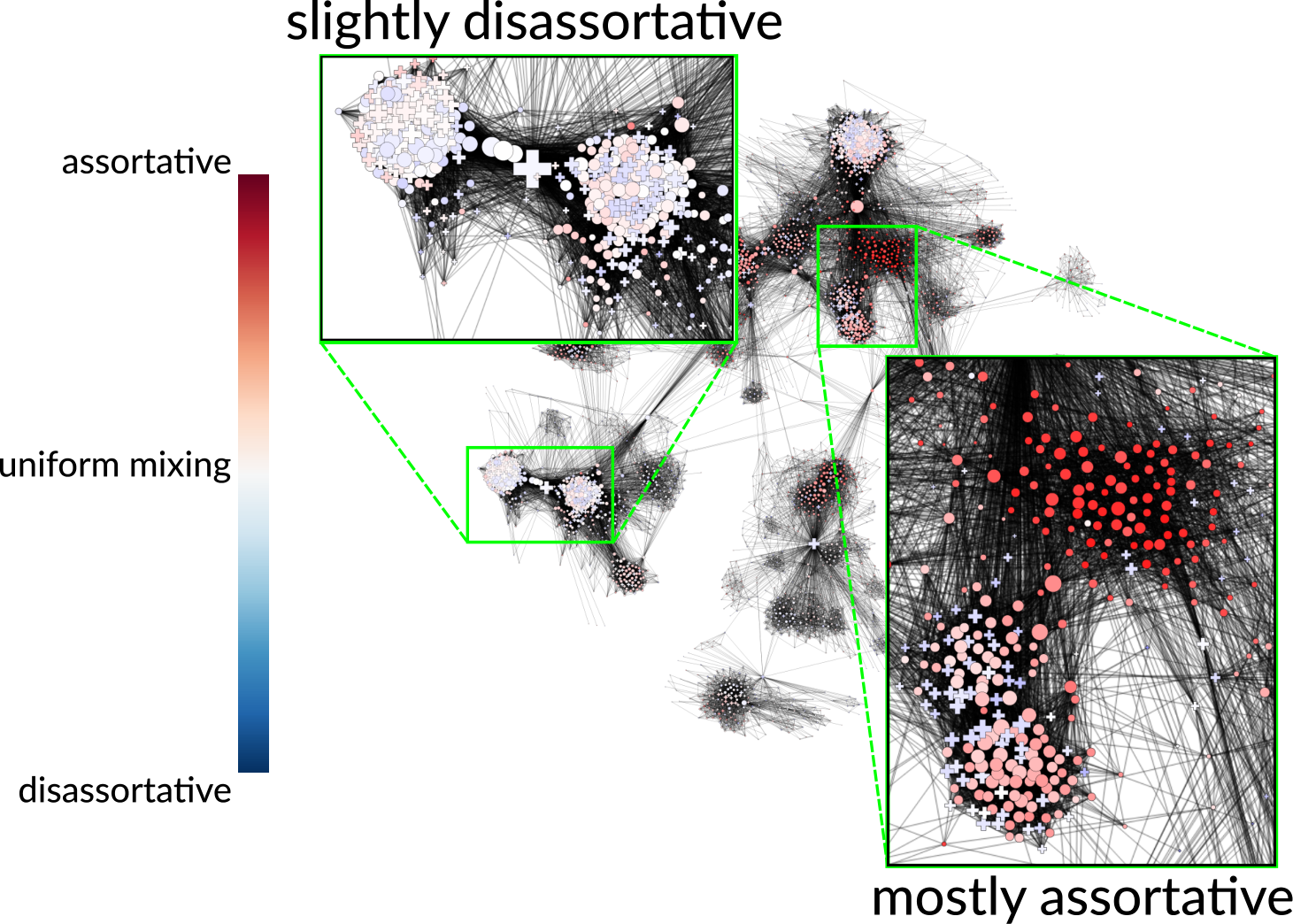
The standard approach to quantifying the level of assortativity in a network is by calculating the assortativity coefficient [13]. Such a summary statistic is useful to capture the average mixing pattern across the whole network. However, such a generalisation is only really meaningful if it is representative of the population of nodes in the network, i.e., if the assortativity of most individuals is concentrated around the mean. But when networks are heterogeneous and contain diverse mixing patterns, a single global measure may not present an accurate description. Furthermore it does not provide a means for quantifying the diversity or identifying anomalous or outlier patterns of interaction.

Quantifying diversity and measuring how mixing may vary across a network becomes a particularly pertinent issue with modern advances in technology that have enabled us to capture, store and process massive-scale networks. Previously social interaction data was collected via time-consuming manual processes of conducting surveys or observations. For practical reasons these were often limited to a specific organisation or group [1, 2, 15, 16]. Summarising the pattern of assortative mixing as a single value may be reasonable for these small-scale networks that tend to focus on a single social dimension (e.g., a specific working environment or common interest). Now, technology such as online social media platforms allow for the automatic collection of increasingly larger amounts of social interaction data. For instance, the largest connected component of the Facebook network was previously reported to account for approximately 10% of the global population [17]. These vast multi-dimensional social networks present more opportunities for heterogeneous mixing patterns, which could conceivably arise, for example, due to differences in demographic and cultural backgrounds. Figure 1 shows, using the methods we will introduce, an example of this variation in mixing on a subset of nodes in the Facebook social network [14]. A high variation in mixing patterns indicates that the global assortativity may be a poor representation of the entire population. To address this issue, we develop a node-centric measure of the assortativity within a local neighbourhood. Varying the size of the neighbourhood allows us to interpolate from the mixing pattern between an individual node and its neighbours to the global assortativity coefficient. In a number of real-world networks we find that the global assortativity is not representative of the collective patterns of mixing.
I Mixing in networks
Currently the standard approach to measure the propensity of links to occur between similar nodes is to use the assortativity coefficient introduced by Newman [13]. Here we will focus on undirected networks and categorical node attributes, but assortativity and the methods we propose naturally extend to directed networks and scalar attributes (see Appendix A & B).
The global assortativity coefficient for categorical attributes compares the proportion of links connecting nodes with same attribute value, or type, relative to the proportion expected if the edges in the network were randomly rewired. The difference between these proportions is commonly known as modularity , a measure frequently used in the task of community detection [18]. The assortativity coefficient is normalised such that if all edges only connect nodes of the same type (i.e., maximum modularity ) and if the number of edges is equal to the expected number for a randomly rewired network in which the total number of edges incident on each type of node is held constant. The global assortativity is given by [13]
| (1) |
in which is half the proportion of edges in the network that connect nodes with type to nodes with type (or the proportion of edges if ) and is the sum of degrees () of nodes with type , normalised by twice the number of edges, . We calculate as:
| (2) |
where is an element of the adjacency matrix. The normalisation constant ensures that the assortativity coefficient lies in the range (see Appendix C).

I.1 Local patterns of mixing
The summary statistic describes the average mixing pattern over the whole network. But as with all summary statistics there may be cases where it provides a poor representation of the network e.g., if the network contains localised heterogeneous patterns. Figure 2 illustrates an analogy to Anscombe’s quartet of bivariate datasets with identical correlation coefficients [19]. Each of the five networks in the top row have the same number of nodes () and edges () and have been constructed to have the same with respect to a binary attribute, indicated by a cross () or a diamond (). All five networks have edges between nodes of the same type and edges between nodes of different types, such that each has . Local patterns of mixing are formed by splitting each of the types further into two equally sized subgroups . The middle row depicts the placement of edges within and between the four subgroups. Distributing edges uniformly between subgroups creates a network with homogeneous mixing [Fig. 2(a)].
We propose a local measure of assortativity that captures the mixing pattern within the local neighbourhood of a given node of interest . Trivially one could calculate the local assortativity by adjusting (1) to only consider the immediate neighbours of . However, taking this approach can encounter problems. For nodes with low degree, we would be calculating assortativity based only on a small sample, providing a potentially poor estimate of the node’s mixing preference. And when all of ’s neighbours are of the same type, then we would assign because .
We face similar issues in time-series analysis when we wish to interpret how a noisy signal varies over time. Direct analysis of the series may be more descriptive of the noise process than the underlying signal we are interested in. Averaging over the whole series provides an accurate estimate of the mean, but treats all variation as noise and ignores any important trends. A common solution to this problem is to use a local filter such as the exponential weighted moving average, in which values further in time from the point of interest are weighted less. We adopt a similar strategy in calculating the local assortativity. To make the connection with time-series analysis concrete, we define a random time-series where each value is the attribute of a node visited in a random walk on the graph. A simple random walker at node jumps to node by selecting an outgoing edge with equal probability, and, in an undirected network, the stationary probability of being at node is proportional to its degree. Then, every edge of the network is traversed in each direction with equal probability . In this context, a key observation is that we can equivalently rewrite (2) as,
| (3) |
which is the total probability that a simple random walker will jump from a node with type to one with type . We can then interpret the global assortativity of the network as the autocorrelation (with time lag of 1) of this random time-series (see Appendix D for details).
Global assortativity counts all edges in the network equally just as the stationary random walker visits all edges with equal probability. To create our local measure of assortativity we instead reweight the edges in the network based on how local they are to the node of interest, . We do so by replacing the stationary distribution in (3) with an alternative distribution over the nodes ,
| (4) |
and compare the proportion of links between nodes of the same type in the local neighbourhood to the global value . Then we can calculate the local assortativity as the deviation from the global assortativity:
| (5) | ||||
| (6) |
All that remains is to define a distribution . We choose the well-known personalised PageRank vector, the stationary distribution of a simple random walk, modified so that at each time step we return to the node of interest with probability [Fig. 3(a)]. In the special case of a network consisting of nodes linked in a line, corresponds to an exponential distribution [Fig. 3(b)] and is analogous to the previously mentioned exponential filter commonly used in time-series analysis. The personalised PageRank vector is an intuitive choice given its role in local community detection [20] and connections to the stochastic block model [21]. It is however, not the only way to define a local neighbourhood (e.g., a number of graph kernels may be suitable [22]), but we leave exploration of other neighbourhood functions for future work.
We can now calculate a local assortativity for each node and use to interpolate from the trivial local neighbourhood assortativity (, the random walker never leaves the initial node) to the global assortativity (, the random walker never restarts) [Fig. 3(c)]. We can also view this local assortativity as a (normalised) autocovariance of the random time-series of node attributes, defined as before but now generated by a stationary random walker with restarts and only when traversing edges of the original network.
I.2 Choice of
We can use to interpolate from the global measure at to the local measure based only on the neighbours of when . As previously mentioned, either extreme can be problematic, is uniform across network, while may be based on a small sample (particularly in the case of low degree nodes) and therefore subject to overfitting. Moreover, both extremes are blind to the possible existence of coherent regions of assortativity inside the network, as considers the network as a whole while considers the local assortativities of the nodes as independent entities.
To circumvent these issues, we consider calculating the assortativity across multiple scales by calculating a “multiscale” distribution by integrating over all possible values of [23],
| (7) |
which is effectively the same as treating as an unknown with a uniform prior distribution (see Appendix H for details). Using this distribution, we can calculate a multiscale measure that captures the assortativity of a given node across all scales.
As a simple demonstration, we return to Figure 2 in which the distribution of for each synthetic network is shown in the bottom row. We see under homogeneous mixing [Fig. 2(a)] a unimodal distribution peaked around confirming that the global measure is representative of the mixing patterns in the network. However, when mixing is heterogeneous [Fig 2(b–e)] we observe multimodal distributions of that allow us to disambiguate between different local mixing patterns.
II Real Networks
Next we use to evaluate the mixing patterns in some real networks: an ecological network and set of online social networks. In both cases nodes have multiple attributes assigned to them, providing different dimensions of analysis.
II.1 Weddell Sea Food Web
We first examine a network of ecological consumer interactions between species dwelling in the Weddell Sea [4]. Figure 4 shows the distributions (green) of local assortativity for five different categorical node attributes. For comparison we present a null distribution (black) obtained by randomly re-wiring the edges such that the attribute values, degree sequence and global assortativity are all preserved (see Appendix I). In each case we observe skewed and/or multi-modal distributions. The empirical distributions appear overdispersed compared to the null distributions.
It may be surprising to see that, for some attributes, the null distribution appears to be multi-modal. Closer inspection reveals that the different modes are correlated with the attribute values and that multi-modality arises from the unbalanced distribution of nodes and incident edges across different node types. This effect is particularly pronounced for the attribute “Metabolic Category” for which we observe two distinct peaks in the distribution. The larger peak that occurs around represents all species that belong to the metabolic category plant and accounts for the majority () of the species in the network, upon which approximately two thirds of the edges are incident. This bias in the distribution of edges across the different node types means that randomly assigned edges are more likely to connect two nodes of the majority class than any other pair of nodes. In fact, it is impossible to assign edges such that nodes in each Metabolic Category exhibit (approximately) the same assortativity as the global value. Specifically, to achieve it is necessary that more than half of the edges connect species from different metabolic categories. However, this is impossible for the plant category without changing the distribution of edges over categories.

II.2 Facebook 100
We next consider a set of online social networks collected from the Facebook social media platform at a time when it was only open to 100 US universities [3]. The process of incrementally providing these universities access to the platform, meant that at this point in time very few links existed between each of the universities’ networks, which provides the opportunities to study each of these social systems in a relatively independent manner. One of the original studies on this dataset examined the assortativity of each demographic attribute in each of the networks [3]. This study found some common patterns that occurred in many of the networks, such as a tendency to be assortative by matriculation year and dormitory of residence, with some variation around the magnitude of assortativity for each of the attributes across the different universities.

In this case it makes sense to analyse the universities separately since it is reasonable to assume that university membership played an important and restricting role in the organisation of the network. However, a modern version of this dataset might contain a higher density of inter-university links, making it less reasonable to treat them independently; in general partitioning networks based on attributes without careful considerations can be problematic [24].
Figure 5 depicts the distributions of for each of the 100 networks according to dormitory. For many of the networks we observe a positively-skewed distribution. The surrounding subplots show details for four universities with approximately the same global assortativity , but with qualitatively different distributions of . Common across these distributions is that all of the empirical distributions exhibit a positive skew beyond that of the null distribution. Closer inspection reveals that in all four networks the nodes associated with a higher local assortativity belong to a community of nodes more loosely connected to the rest of the network. These nodes also correspond to first-year students, which suggests that residence is more relevant to friendship among new students than it is for the rest of the student body. We see this pattern in many of the other schools too, first-year students are more assortative by year (for all schools except one) and by residence (more than 75% of schools), see Figs. 8 & 9 in the Appendix for details.
We can also use local assortativity to compare how the mixing of multiple attributes covary across a network. This may be of interest as a positive correlation could suggest a relationship between attributes, while a negative correlation indicates that assortativity of one attribute may replace the assortativity of another. Note that differences in normalisation between attributes mean that the actual values may not be directly comparable, which is why we focus on correlation. Figure 6 compares for year of study and place of residence. The central scatter plot shows, for each university: the correlation between local assortativities of the two attributes (x-axis) against the difference in the two global assortativities for each network (y-axis), which was previously the only way to compare assortativities [3]. The four surrounding sub-plots show the joint distribution of year and dorm local assortativity for specific universities. The yellow points indicate students in their first year. In most universities we observed that first-year students were the most assortative by either year, residence or both. In both Auburn and Pepperdine there is a negative correlation between year and dorm assortativity suggesting that many friendships are associated with either being in the same year or from sharing a dorm.
For Simmons and Rice we observe a positive correlation between dorm and year local assortativity. However, in Simmons we see that the first-year students form a separate cluster, while in Rice they are much more interspersed. This difference may relate to how students are placed in university dorms. At Simmons all first year students live on campus11 1 source:http://www.simmons.edu/student-life/life-at-simmons/housing/residence-halls and form the majority residents in the few dorms they occupy. Rice houses their new intakes according to a different strategy, by placing them evenly spread across all the available dorms. The fact that students are mixed across years and that the vast majority (almost 78%22 2 source:http://campushousing.rice.edu/) of students reside in university accommodation, offers a possible explanation for why we observe a smooth variation in values of assortativity without a distinction between new students and the rest of the population.
III Discussion
Characterising the level of assortativity plays an important role in understanding the organisation of complex systems. However, the global assortativity may not be representative given the variation present in the network. We have shown that the distribution of mixing in real networks can be skewed, overdispersed and possibly multimodal. In fact, for certain network configurations we have seen that a unimodal distribution may not even be possible.
As network data grow bigger there is a greater possibility for heterogeneous sub-groups to co-exist within the overall population. The presence of these sub-populations adds further to the ongoing discussions of the interplay between node metadata and network structure [24] and suggests that while we may observe a relationship between particular node properties and existence of links in part of a network, it does not imply that this relationship exists across the network as a whole. This heterogeneity has implications on how we make generalisations in network data, as what we observe in a subgraph might not necessarily apply to the rest of the network. However, it may also present new opportunities too. Recent results show that with an appropriately constructed learning algorithm it is still possible to make accurate predictions about node attributes in networks with heterogeneous mixing patterns [25] and in some cases even utilise the heterogeneity to further improve performance [26]. Quantifying local assortativity offers a new dimension to study this predictive performance. Heterogeneous mixing also offers a potential new perspective for the community detection problem [27], i.e., to identify sets of nodes with similar assortativity, which may be useful in the study of “echo chambers” in social networks [28].
Our approach to quantifying local mixing could easily be applied to any global network measure, such as clustering coefficient or mean degree. It may also be used to capture the local correlation between node attributes and their degree, a relationship that plays a definitive role in network phenomena such as the majority illusion [29] and the generalised friendship paradox [30].
Acknowledgements
This work was supported by ARC (Federation Wallonia-Brussels) [LP, JCD, RL] and FNRS-F.R.S. [LP].
References
- [1] David Krackhardt, “The ties that torture: Simmelian tie analysis in organizations,” Research in the Sociology of Organizations 16, 183–210 (1999).
- [2] Emmanuel Lazega, The collegial phenomenon: The social mechanisms of cooperation among peers in a corporate law partnership (Oxford University Press, 2001).
- [3] Amanda L Traud, Peter J Mucha, and Mason A Porter, “Social structure of facebook networks,” Physica A 391, 4165–4180 (2012).
- [4] Ulrich Brose et al., “Body sizes of consumers and their resources,” Ecology 86, 2545 (2005).
- [5] H Jeong, B Tombor, R Albert, ZN Oltvai, and AL Barabasi, “The large-scale organization of metabolic networks,” Nature 407, 651 (2000).
- [6] Réka Albert, Hawoong Jeong, and Albert-László Barabási, “Internet: Diameter of the world-wide web,” Nature 401, 130 (1999).
- [7] Duncan J Watts and Steven H Strogatz, “Collective dynamics of ’small-world’ networks,” Nature 393, 440 (1998).
- [8] Miller McPherson, Lynn Smith-Lovin, and James M Cook, “Birds of a feather: Homophily in social networks,” Annu. Rev. Sociol. 27, 415–444 (2001).
- [9] Sinan Aral, Lev Muchnik, and Arun Sundararajan, “Distinguishing influence-based contagion from homophily-driven diffusion in dynamic networks,” Proc. Natl. Acad. Sci. 106, 21544–21549 (2009).
- [10] James Moody, “Race, school integration, and friendship segregation in america,” Am. J. Sociol. 107, 679–716 (2001).
- [11] Jere M Cohen, “Sources of peer group homogeneity,” Sociol Educ , 227–241 (1977).
- [12] Denise B Kandel, “Homophily, selection, and socialization in adolescent friendships,” Am. J. Sociol. 84, 427–436 (1978).
- [13] Mark EJ Newman, “Mixing patterns in networks,” Phys. Rev. E 67, 026126 (2003).
- [14] Julian J McAuley and Jure Leskovec, “Learning to discover social circles in ego networks,” in Adv. Neur. In. 25, Vol. 2012 (2012) pp. 539–547.
- [15] Samuel F Sampson, A novitiate in a period of change: An experimental and case study of social relationships, Ph.D. thesis, Cornell University Ithaca, NY (1968).
- [16] Wayne W Zachary, “An information flow model for conflict and fission in small groups,” J. Anthropol. Res. , 452–473 (1977).
- [17] Johan Ugander, Brian Karrer, Lars Backstrom, and Cameron Marlow, “The anatomy of the facebook social graph,” preprint arXiv:1111.4503 (2011).
- [18] Mark EJ Newman and Michelle Girvan, “Finding and evaluating community structure in networks,” Phys. rev. E 69, 026113 (2004).
- [19] Francis J Anscombe, “Graphs in statistical analysis,” Am. Stat. 27, 17–21 (1973).
- [20] Reid Andersen, Fan Chung, and Kevin Lang, “Local graph partitioning using pagerank vectors,” in Foundations of Computer Science (FOCS’06) (IEEE, 2006) pp. 475–486.
- [21] Isabel M Kloumann, Johan Ugander, and Jon Kleinberg, “Block models and personalized pagerank,” Proc. Natl. Acad. Sci. 114, 33–38 (2016).
- [22] François Fouss, Marco Saerens, and Masashi Shimbo, Algorithms and models for network data and link analysis (Cambridge University Press, 2016).
- [23] Paolo Boldi, “Totalrank: Ranking without damping,” in Special interest tracks and posters of the 14th international conference on World Wide Web (WWW) (ACM, 2005) pp. 898–899.
- [24] Leto Peel, Daniel B Larremore, and Aaron Clauset, “The ground truth about metadata and community detection in networks,” Sci. Adv. 3, e1602548 (2017).
- [25] Leto Peel, “Graph-based semi-supervised learning for relational networks,” in SIAM International Conference on Data Mining (SIAM, 2017) pp. 435–443.
- [26] Kristen M Altenburger and Johan Ugander, “Bias and variance in the social structure of gender,” preprint arXiv:1705.04774 (2017).
- [27] Michael T Schaub, Jean-Charles Delvenne, Martin Rosvall, and Renaud Lambiotte, “The many facets of community detection in complex networks,” Applied Network Science 2, 4 (2017).
- [28] Elanor Colleoni, Alessandro Rozza, and Adam Arvidsson, “Echo chamber or public sphere? predicting political orientation and measuring political homophily in twitter using big data,” J. Commun. 64, 317–332 (2014).
- [29] Kristina Lerman, Xiaoran Yan, and Xin-Zeng Wu, “The” majority illusion” in social networks,” PloS one 11, e0147617 (2016).
- [30] Young-Ho Eom and Hang-Hyun Jo, “Generalized friendship paradox in complex networks: The case of scientific collaboration,” Sci. Rep. 4, srep04603 (2014).
- [31] George Udny Yule, “On the methods of measuring association between two attributes,” J. R. Stat. Soc. 75, 579–652 (1912).
- [32] George A Ferguson, “The factorial interpretation of test difficulty,” Psychometrika 6, 323–329 (1941).
- [33] Joy Paul Guilford, Fundamental statistics in psychology and education. (McGraw-Hill, 1950).
- [34] Ernest C Davenport Jr and Nader A El-Sanhurry, “Phi/phimax: review and synthesis,” Educ. Psychol. Meas. 51, 821–828 (1991).
- [35] Edward E. Cureton, “Note on /max,” Psychometrika 24, 89–91 (1959).
- [36] Jacob Cohen, “A coefficient of agreement for nominal scales,” Educ Psychol Meas 20, 37–46 (1960).
- [37] Paolo Boldi, Massimo Santini, and Sebastiano Vigna, “A deeper investigation of pagerank as a function of the damping factor,” in Web Information Retrieval and Linear Algebra Algorithms, 07071 (2007).
- [38] Bailey K Fosdick, Daniel B Larremore, Joel Nishimura, and Johan Ugander, “Configuring random graph models with fixed degree sequences,” preprint arXiv:1608.00607 (2016).
Appendix A Directed networks
We can easily extend the multiscale mixing measure described in the main text to directed networks. The main change is to incorporate two sets of marginals and that describe the proportion of edges starting from and ending at each of the attribute types. Then the directed global assortativity of a network with respect to a particular categorical node attribute is:
| (8) |
where and represent the total number of outgoing and incoming links of all nodes of type :
| (9) |
Then we can update our definition of local assortativity accordingly,
| (10) |
Appendix B Scalar attributes
For scalar attributes we can simply calculate the Pearson’s correlation across edges. Using and to indicate the scalar attribute value of the nodes in edge then we can write the global assortativity as,
| (11) | ||||
| (12) |
where is the mean value of weighted by node degree and is the standard deviation of the attribute values. If we standardise the scalar values using the linear transformation , then we can simplify this further as,
| (13) |
Then we can calculate the local assortativity for scalar variables as,
| (14) |
Figure 7 gives some examples of distributions of for scalar attributes in the food web network.
Appendix C Categorical assortativity as a correlation
The assortativity coefficient for categorical attributes can be interpreted as a normalised Pearson’s correlation. To see this, we start by observing that the Pearson’s correlation of two binary variables is equivalent to the Phi coefficient for binary contingency tables [31]. Table 1 shows a contingency table using the same notation as the directed assortativity, i.e., and give the marginal proportions and gives the joint proportions.
Then the Pearson product-moment correlation of these variables is known as , which we derive using the moments of a Bernoulli distribution:
| (15) | ||||
| (16) |
Note that it is only necessary to calculate this in terms of , since . We can see this using the identity :
| (17) | ||||
| (18) | ||||
| (19) |
A well-known issue with is that the extreme values of and are typically unobtainable, which can cause issues with its interpretation. In fact can only occur if , e.g., when the network is undirected, while can only occur if [32, 33]. To address this issue, there have been a number of proposed normalisations to ensure the is obtainable [34]. One such normalisation is the proposed by Cureton [35],
| (20) |
where is the maximum possible value that can take, i.e., . Note for undirected networks
| (21) | ||||
| (22) | ||||
| (23) | ||||
| (24) |
which equals wnen .
Then we can generalise from binary to multi-category variables by treating each distinct value as a binary variable and taking their sum. If we set , then we obtain (8) and thus we recover Newman’s assortativity [13]. We also note that (8) also corresponds to Cohen’s that is frequently used to assess inter-rater agreement [36].
The normalisation of the assortativity coefficient means that and
| (25) |
which lies in the range .
Appendix D Assortativity as autocorrelation of a time-series
Assume a scalar attribute on each node of an undirected network. As mentioned in the main text, the probability of being at node is stationary and proportional to the degree, . Given that a random walker is currently at node , it moves to node with probability .
We define a random time-series, using the simple random walker, as the sequence of attributes of the nodes visited in the random walk, i.e., the value of the time series at time is the attribute value of the node visited at time in the random walk. Asymptotically, the average value observed by the random walker is and the variance is .
Likewise, the autocovariance between the attribute observed at two consecutive steps (time lag of 1) is . Replacing by , we obtain the autocorrelation , which coincides with as defined in (13).
When faced with categorical data, we proceed as in SI C. We consider for each type of nodes the scalar attribute valued at 1 for nodes with type and zero elsewhere. The modularity is therefore the sum for each type of the autocovariance, . As in SI C, this can be normalised in various ways, one of which is Newman’s global assortativity as used in this article, which therefore represents a sort of categorical autocorrelation of the time-series process of the categorical attributes observed by the stationary simple random walker.
Appendix E Disconnected networks
By using the personalised PageRank as a neighbourhood function it means that only nodes within the same connected component contribute to . Consequently for each node is insensitive to whether or not multiple connected components are included.
Appendix F Missing values
It is common when dealing with real datasets that some values may be missing. This is the case for the Facebook100 data, where a number of node attributes are missing. When considering the global assortativity previous work has simply ignored contributions from missing data values [3]. That is, only edges that connect nodes for which both the attribute values are known are considered when calculating . This treatment works fine for the global assortativity because each edge counts equally. However, simply omitting missing values when calculating the local assortativity can cause a bias in the distribution. For example, consider the case when node and its immediate neighbours have missing values, but beyond those the attribute values are known. For small values of the weight is largest for nodes with missing attribute values. Simply ignoring their edges would mean reassigning more weight to edges further away from when normalising to ensure that , a necessary step in calculating the assortativity. Then when we examine the distribution of across all nodes in the network, the resulting distribution will be biased representation. To deal with this issue we calculate each of the local assortativities as normal, but assign each a weight , i.e., the sum of local edge counts before normalisation. The weight describes our confidence in the local assortativity estimate from , indicating no confidence, to when all node attributes within the neighbourhood are known. We adjust for these weights when plotting the histograms in the main text.
Appendix G Calculating the personalised PageRank vector
The personalised PageRank vector is the stationary distribution of a random walk with restarts. We calculate it by direct simulation of the random walk process using the power method:
| (26) |
and at convergence yields a distribution with a mode at .
Appendix H Integrating over
To integrate over all values of , we take advantage of the fact that we can equivalently write the -th approximation the power method in (26) as the -th degree truncation of the power series [37]:
| (27) |
By taking advantage of the relationship between and the sequence of approximations computed by the power method, we can calculate the distribution for a given and use the sequence of approximations to calculate the distribution for any other [37]:
| (28) |
We can then integrate over all possible values of [23],
| (29) | ||||
| (30) |
Appendix I Null model network generation
We created a null model to generate networks with the same global assortativity as the observed network to compare the distributions of . For a fair comparison, we decided to keep the node degree and metadata label fixed while randomly rewiring the network. We do so using a modified version of the Markov chain Monte Carlo (MCMC) sampling of the configuration model for stub-labelled33 3 for simple graphs sampling from the space of stub-labelled graphs is equivalent to sampling from the space of vertex-labelled graphs [38] simple graphs [38]. The modification is to ensure that we sample a graph with (approximately) the same global assortativity as the observed network. We achieve this by adding a rejection sampling step based on the binomial likelihood of observing the number of edges between nodes of the same type given the proportion of edges required to maintain the global assortativity ,
| (31) |
The modified MCMC algorithm is shown in Algorithm 1
Appendix J Datasets
J.1 Weddell Sea Food Web
The food web of the Antarctic Weddell Sea [4] consists of 488 species and 15885 consumer relations. For each of the nodes in this network we have five categorical attributes: Metabolic Category {Plant, Ectotherm vertebrate, Endotherm vertebrate, Invertebrate}, Feeding Type {Carnivorous/necrovorous, Herbivorous/detrivorous, Detrivorous, Omnivorous, Primary producer, Carnivorous}, FeedingMode {Pelagic predator, Predator/scavenger, Primary producer, Predator, Deposit-feeder, Grazer, Suspension-feeder}, Mobility , Environment {Bathydemersal, Land-based, Resource, Pelagic, Benthopelagic, Benthic, Demersal}. For scalar attributes we use the mean mass of the species, mobility (although discrete, the values are ordinal), and node degree.
J.2 Facebook 100
The Facebook100 dataset [3] contains an anonymised snapshot of the friendship connections among users affiliated with the first 100 colleges admitted to Facebook. The dataset contains a total of friendship edges between users of the same college. Each node has a set of categorical social variables: status {undergraduate, graduate student, summer student, faculty, staff, alumni}, dorm, major, gender {male, female}, and graduation year.
| # | School | # | School | ||
|---|---|---|---|---|---|
| 1 | Amherst 41 | 0.081 | 51 | William 77 | 0.203 |
| 2 | Princeton 12 | 0.087 | 52 | Emory 27 | 0.205 |
| 3 | Trinity 100 | 0.106 | 53 | UCLA 26 | 0.208 |
| 4 | Stanford 3 | 0.109 | 54 | Tennessee 95 | 0.209 |
| 5 | Swarthmore 42 | 0.109 | 55 | Wake 73 | 0.212 |
| 6 | Johns Hopkins 55 | 0.110 | 56 | MIT 8 | 0.219 |
| 7 | Hamilton 46 | 0.113 | 57 | UMass 92 | 0.222 |
| 8 | Bowdoin 47 | 0.118 | 58 | Berkeley 13 | 0.222 |
| 9 | Harvard 1 | 0.120 | 59 | USC 35 | 0.224 |
| 10 | Brown 11 | 0.120 | 60 | Temple 83 | 0.228 |
| 11 | Dartmouth 6 | 0.126 | 61 | UVA 16 | 0.230 |
| 12 | Wellesley 22 | 0.127 | 62 | Penn 94 | 0.231 |
| 13 | Haverford 76 | 0.128 | 63 | Northwestern 25 | 0.234 |
| 14 | Wesleyan 43 | 0.128 | 64 | Rutgers 89 | 0.235 |
| 15 | UConn 91 | 0.129 | 65 | UPenn 7 | 0.235 |
| 16 | Tufts 18 | 0.130 | 66 | Michigan 23 | 0.236 |
| 17 | Williams 40 | 0.133 | 67 | FSU 53 | 0.238 |
| 18 | Reed 98 | 0.134 | 68 | Cornell 5 | 0.238 |
| 19 | Columbia 2 | 0.136 | 69 | UC 64 | 0.251 |
| 20 | BC 17 | 0.136 | 70 | American 75 | 0.253 |
| 21 | Duke 14 | 0.144 | 71 | Notre Dame 57 | 0.255 |
| 22 | Virginia 63 | 0.149 | 72 | Rochester 38 | 0.256 |
| 23 | Oberlin 44 | 0.151 | 73 | Vassar 85 | 0.256 |
| 24 | Villanova 62 | 0.158 | 74 | Lehigh 96 | 0.258 |
| 25 | Howard 90 | 0.159 | 75 | Texas 80 | 0.261 |
| 26 | WashU 32 | 0.162 | 76 | USFCA 72 | 0.263 |
| 27 | Georgetown 15 | 0.162 | 77 | UC 61 | 0.265 |
| 28 | Colgate 88 | 0.164 | 78 | Syracuse 56 | 0.270 |
| 29 | UF 21 | 0.165 | 79 | Yale 4 | 0.273 |
| 30 | BU 10 | 0.167 | 80 | UCSB 37 | 0.277 |
| 31 | Carnegie 49 | 0.171 | 81 | Cal 65 | 0.279 |
| 32 | GWU 54 | 0.171 | 82 | Texas 84 | 0.291 |
| 33 | Bingham 82 | 0.176 | 83 | UChicago 30 | 0.291 |
| 34 | NYU 9 | 0.182 | 84 | Smith 60 | 0.292 |
| 35 | UNC 28 | 0.185 | 85 | Mississippi 66 | 0.297 |
| 36 | Simmons 81 | 0.186 | 86 | Baylor 93 | 0.297 |
| 37 | USF 51 | 0.187 | 87 | UIllinios 20 | 0.297 |
| 38 | JMU 79 | 0.187 | 88 | MU 78 | 0.306 |
| 39 | UCF 52 | 0.187 | 89 | Tulane 29 | 0.313 |
| 40 | Santa 74 | 0.188 | 90 | Mich 67 | 0.322 |
| 41 | Northeastern 19 | 0.190 | 91 | UGA 50 | 0.336 |
| 42 | Maine 59 | 0.190 | 92 | Wisconsin 87 | 0.338 |
| 43 | Middlebury 45 | 0.190 | 93 | UCSD 34 | 0.355 |
| 44 | Brandeis 99 | 0.193 | 94 | Indiana 69 | 0.356 |
| 45 | Bucknell 39 | 0.194 | 95 | UC 33 | 0.361 |
| 46 | MSU 24 | 0.195 | 96 | Auburn 71 | 0.370 |
| 47 | Pepperdine 86 | 0.198 | 97 | Oklahoma 97 | 0.397 |
| 48 | Vermont 70 | 0.199 | 98 | Caltech 36 | 0.426 |
| 49 | Maryland 58 | 0.199 | 99 | UCSC 68 | 0.480 |
| 50 | Vanderbilt 48 | 0.201 | 100 | Rice 31 | 0.504 |

