Robust causal structure learning with some hidden variablesThanks: BF and PN are equally contributing authors.
Abstract.
We introduce a new method to estimate the Markov equivalence class of a directed acyclic graph (DAG) in the presence of hidden variables, in settings where the underlying DAG among the observed variables is sparse, and there are a few hidden variables that have a direct effect on many of the observed ones. Building on the so-called low rank plus sparse framework, we suggest a two-stage approach which first removes the effect of the hidden variables, and then estimates the Markov equivalence class of the underlying DAG under the assumption that there are no remaining hidden variables. This approach is consistent in certain high-dimensional regimes and performs favourably when compared to the state of the art, both in terms of graphical structure recovery and total causal effect estimation.
Key words and phrases:
directed acyclic graphs (DAGs), causal structure learning, causality, confounding, structured sparsity, high-dimensional consistency1. Introduction
The task of learning causal directed acyclic graphs (causal DAGs) arises in many areas of science and engineering. In such graphs, nodes represent random variables and edges encode direct causal effects. The problem of recovering their structure from observational data is challenging and cannot be tackled without making untestable assumptions [39]. Among other assumptions, causal sufficiency is particularly constraining. Briefly, causal sufficiency requires that there be no hidden (or latent) variables that are common causes of two or more observed variables (such hidden variables are often called confounders). Although causal sufficiency is unrealistic in most applications, many structure causal learning algorithms operate under this assumption (e.g. [46, 8, 51, 37]). On the other hand, methods allowing for arbitrary hidden structures tend to be overly conservative, recovering only a small subset of the causal effects [47, 11, 9]. In the present work, we suggest taking a middle-ground stance on causal sufficiency by allowing hidden variables while imposing some restrictions on their number and behaviour. More precisely, we consider settings where the underlying DAG among the observed variables is sparse, and there are a few hidden variables that have a direct effect on many of the observed ones [6]. This is an interesting problem for at least two reasons.
First, these assumptions cover important real-world applications. In the context of gene expression data, for example, such confounding occurs due to technical factors or unobserved environmental variables (e.g. [29, 49, 18]). For another example, consider the task of modelling the inverse covariance structure of stock returns [23, §9.5]. [6] showed that a large fraction of the conditional dependencies among stock returns can be explained by a few hidden variables, e.g. energy prices. By applying similar ideas to the modelling of the California reservoir network, [50] were able to infer and quantify the effect of external phenomena that have a system-wide effect on the network.
Second, this setting is complementary to the realm of application of popular algorithms that do not assume causal sufficiency, such as versions of the Fast Causal Inference algorithm [47, 11, 9]. Under our assumption that there are a few hidden variables that affect many of the observed ones, most observed variables are conditionally dependent given any subset of the observed variables. Hence, the underlying so-called maximal ancestral graph is expected to be dense which, in turn, implies that very few edges can be oriented (see Figure 1 for an example). Moreover, learning such dense graphs is computationally demanding.
In this paper, we suggest a two-stage procedure. First, the so-called “low-rank plus sparse” approach of [6] is applied to the covariance matrix to obtain a pair of positive semi-definite matrices, say, describing the estimated inverse covariance matrix between observed variables conditional on the hidden ones (), and the estimated effect of the hidden variables (). In the second stage, a causal structure learning algorithm which assumes causal sufficiency is applied to . In addition, (joint) total causal effects can be straightforwardly estimated using the (joint-)IDA algorithm [34, 32, 38].
The suggested approach is conceptually simple and enjoys many desirable theoretical and computational properties. We study two versions of our estimator. One is based on the sample covariance matrix, as described above, and the other on the sample Kendall correlation matrix. Building on recent work by [54] and [19], we first establish the convergence rates of the low-rank plus sparse approach for two families of distributions – sub-Gaussian random variables and transelliptical distributions – thus extending previous results which assumed Gaussian distributions. We then derive conditions and scaling regimes under which our two stage estimators are consistent. Through extensive simulations, we show that our approach outperforms other relevant methods, both in terms of graph structure recovery and total causal effect estimation. Our main focus being on applicability, we also suggest strategies to select the tuning parameters in various settings and illustrate their performances in simulations. Finally, we analyse two datasets. In our first application, we model the expression levels of the genes responsible for isoprenoid synthesis in Arabidopsis thaliana and show that some of the hidden variables we estimate have a clear biological interpretation. We also model the expression levels of hundreds of genes expressed in ovarian cancer and assess our results using two external sources of validation. Compared to state-of-the-art algorithms, we find our approach to be better at recovering known causal relationships11 1 The code for our simulations and applications is made available with this paper..
2. Preliminaries
2.1. Graphical Models Terminology
We consider graphs , where the vertices (or nodes) represent random variables and the edges represent relationships between pairs of variables. The edges can be either directed () or undirected (). A directed graph can only contain directed edges. An undirected graph can only contain undirected edges. A partially directed graph may contain both directed and undirected edges. The skeleton of a partially directed graph , denoted as , is the undirected graph that results from replacing all directed edges of by undirected edges.
Two nodes and are adjacent if there is an edge between them. If , then is a parent of . A path between and in a graph is a sequence of distinct nodes such that all pairs of successive nodes in the sequence are adjacent in . A directed path from to is a path between and , where all edges are directed towards . A directed path from to together with forms a directed cycle. A graph without directed cycles is acyclic. A graph that is both (partially) directed and acyclic, is a (partially) directed acyclic graph or (P)DAG.
A DAG encodes conditional independence relationships via the notion of d-separation [see 40, Def. 1.2.3]. Several DAGs can encode the same set of d-separations and such DAGs form a Markov equivalence class. A Markov equivalence class of DAGs can be uniquely represented by a completed partially directed acyclic graph (CPDAG), which is a PDAG that satisfies the following: in the CPDAG if in every DAG in the Markov equivalence class, and in the CPDAG if the Markov equivalence class contains a DAG in which as well as a DAG in which [52, 3]. In this sense, the circle marks represent uncertainty about the edge marks.
For , we write to denote that and are independent given , while means that and are d-separated by in . A DAG is a perfect map of the joint distribution of if for all such that and for all , we have .
When some variables are unobserved, as is assumed in this paper, complications arise because the class of DAGs is not closed under marginalisation. Among other factors, this limitation prompted the development of another class of graphical independence models called maximal ancestral graphs (MAGs) [43]. A criterion akin to d-separation makes it possible to read-off independencies of such graphs and, since multiple MAGs can encode the same set of conditional independence statements, one usually attempts to recover a partial ancestral graph (PAG) which describes a Markov equivalence class of MAGs [2]. Like in CPDAGs, circle marks represent uncertainty about edge marks. In particular, a circle mark occurs in the PAG if the Markov equivalence class contains a MAG in which the edge mark is a tail, and a MAG in which the edge mark is an arrowhead [56].
2.2. Background on sub-Gaussian Random Variables and Transelliptical Distributions
In what follows, we will consider structural equation models with errors that are either sub-Gaussian or elliptical.
A random variable is sub-Gaussian if the tails of its distribution decay at least as fast as the tails of a Gaussian distribution. Formally, a random variable is said to be sub-Gaussian with parameter if and it satisfies
A random vector is sub-Gaussian with parameter if and is sub-Gaussian with parameter for all unit vectors . Important examples of sub-Gaussian random variables are Gaussian random variables, Bernoulli random variables and, more generally, any bounded random variable. We refer the reader to [53] for more results and definitions about sub-Gaussian random variables, including the notion sub-Gaussian norm.
An elliptical distribution is another extension of the multivariate Gaussian distribution. For any two random vectors and , let denote the fact that and have the same distribution. Then, a random vector is said to have an elliptical distribution if and only if has stochastic representation (Def. 2.1 in [19]). Here, , , , is a random variable independent of , is uniformly distributed on the unit sphere in . Letting , we write . We limit ourselves to those distributions for which , thus guaranteeing the existence of the covariance matrix which is then equal to . Any linear combination of elliptically distributed variates is still elliptical. More precisely, for , and , we have (Th. 2.16 of [15]). Interesting examples of elliptical distributions include the family of multivariate -distributions (with 3 or more degrees of freedom) and rank-deficient Gaussians. We will however assume that is non-singular.
Transelliptical distributions – or semiparametric elliptical copulas – extend elliptical distributions in that they allow for some marginal transformations of the random variables. A random vector follows a transelliptical distribution (Def. 2.2 in [19]) if there exist strictly increasing univariate functions such that
We write . Following the terminology of [30], is called the latent generalised correlation matrix. Moreover, the family of transelliptical distributions – and a fortiori the family of elliptical distributions – is closed under marginalisation and conditioning (Lemma 3.1 [30]), a property which allows the definition of so-called transelliptical graphical models.
3. Problem Statement and Suggested Work
3.1. Setup and Notations
Throughout, we assume that we are given independent, identically distributed (i.i.d.) realisations of a partially observed, zero-mean random vector , where the variables in are observed while the variables in remain hidden. We consider two distinct settings:
- (Setting 1):
-
either is jointly sub-Gaussian with inverse covariance matrix , and there exists a DAG, say, which is a perfect map of the distribution of conditional on . It is assumed that the causal mechanism generating conditional on is of the form
(1) We assume that an intervention on observed variables has no effect on the distribution of . The non-zero pattern of is determined by the causal DAG . Furthermore, is diagonal and is a sub-Gaussian random vector which is independent of .
- (Setting 2):
-
or is transelliptically distributed according to with , and there exists a DAG, say, which is a perfect map of the distribution of conditional on . It is assumed that the causal mechanism generating conditional on is of the form
(2) We assume that an intervention on observed variables has no effect on the distribution of . Here, and satisfy the same assumptions as in Setting 1, except that we relax the sub-Gaussian assumption while imposing the assumption that is an elliptically distributed random vector.
One possible interpretation of (1) and (2) is that they describe linear structural equation models (SEMs) with correlated errors. We now look at these settings more closely. Let be partitioned as follows
with , , . The conditional distribution of given is sub-Gaussian with covariance matrix or transelliptical with latent generalised correlation matrix . We assume that there exists a DAG which is a perfect map of a sub-Gaussian distribution with covariance matrix (Setting 1) or a perfect map of an elliptical distribution with correlation matrix (Setting 1). Our goal is to estimate and the CPDAG that represents Markov equivalence class of . These estimates can be used in estimating causal effects between observed variables. In fact, under the causal model described by (1), one can show that the causal effect of on equals the regression coefficient of in the linear regression of on and ’s parents in , computed from (see, for example, Proposition 3.1 of the supplementary material of [38]). Similar result holds for the causal model described by (2). Hence, estimates of and enable the estimation of multisets of possible causal effects, via the (joint-)IDA algorithm [34, 33, 38].
Since is unobserved, we need to estimate and from i.i.d. samples from the marginal distribution of . A simple calculation yields for Setting 1 that is sub-Gaussian with , and for Setting 2 that (see, for example, Corollary of Th. 2.16 in [15]). Setting , we have that summarises the effect of the hidden variables on the observed ones. In practice, only samples from these marginal distributions are observed and we let be some generic estimator of . For example, could be the sample covariance matrix (Setting 1) or a modified sample Kendall correlation matrix (Setting 2). In what follows, conditions on and will be given for estimating consistently under Settings 1 and 2. We will then use the estimate of to obtain a consistent estimate under further assumptions.
To make Settings 1 and 2 easier to comprehend, consider a set of hidden variables such that is generated from an acyclic linear SEM with uncorrelated errors:
where is a sub-Gaussian random vector with . Then it follows from straightforward calculation that satisfies Setting 1 with , , and equals the DAG that corresponds to the non-zero entries in . A similar result holds for Setting 2 with .
If we additionally assume in (3.1), then we have and equals or . The assumption restricts ourselves to linear SEMs where hidden variables do not have observed parents. From a mathematical point of view, this assumption is not necessary. When it holds, however, a qualitative interpretation of our conditions on and required for consistently estimating is possible. Namely, that there be few hidden variables with widespread effects and that there be few direct causes of each observed variable.
In Figure 1 a) an example of a DAG with two influential hidden variables is given. In such a scenario, the MAG and PAG (Fig. 1 b), c)) are dense and the PAG contains many uninformative circle edgemarks. For comparison, Figure 1 d) depicts our target object which is sparse and contains more informative edge marks.
a)
b)
c)
d)
We will use the following standard notations. For an arbitrary matrix , denotes the sum of its entries’ magnitudes; is the sum of its singular values; is its largest entry in magnitude; is its largest singular value; is the Frobenius norm. In addition, for a symmetric matrix , (resp. ) indicates that is positive definite (resp. positive semi-definite). We denote by the maximum number of non-zero entries in any row or column of . If is a partially directed graph and is the adjacency matrix of its skeleton, we define its degree as .
3.2. Suggested Estimators
In this section, we discuss methods for estimating and under Settings 1 and 2. To this end, we first discuss the problem of estimating . Recall that we denote the marginal covariance matrix of by , and that its inverse equals . Even in the absence of noise, inferring the components of is a challenging problem because it is fundamentally misspecified: an infinity of pairs satisfy the equation under the constraints , .
For an arbitrary matrix such that , the problem of recovering and from or an estimate of has been studied when is sparse and is dense and of low-rank [5, 7]. Loosely speaking, they showed that is with high probability equal to the solution of the convex problem,
| (11) |
provided is chosen within a suitable interval. The form taken by (11) is motivated by the fact that the and nuclear norms are convex relaxations for the -norm and the rank respectively. The penalties on and encourage the learning of a sparse and a low-rank , while the tuning parameter adjusts the relative weight of these two penalties. In the special case of multivariate Gaussian distributions, [6] showed that it is also possible to recover and when only samples from the marginal distribution of are available. In this context, the assumption that is dense and low-rank means that there must be relatively few hidden variables with an effect spread over most of the observed variables. An estimate of is obtained as the minimiser of a function which couples the Gaussian log-likelihood: with (11)
| (12) |
where and . Here, the Gaussian log-likelihood makes it possible to learn an inverse covariance from the sample covariance , while the penalty plays the double role of regularising the likelihood to prevent singularities (via ) and decomposing the estimated precision matrix into its components. The objective function in (12) is jointly convex in its parameters and can be efficiently minimised even when is in the thousands [31]. We call this estimator the “low-rank plus sparse” estimator (LRpS) and we write for the program which applies (12) to a positive semi-definite matrix , with tuning parameters and outputs a pair of matrices .
When the random variables are jointly Gaussian, zero partial correlation and conditional independence are equivalent. This puts the edges of a Gaussian graphical model and the non-zero entries of the precision matrix in a one-to-one correspondence [28]. This property is desirable but is not necessary for (12) to consistently estimate – and therefore irrelevant to the problem at hand. All that is required is a consistent estimator of . When the errors are sub-Gaussian, the sample covariance matrix is such an estimator [53]. For heavy-tailed distributions, a modified Kendall correlation matrix can be used [30].
Provided the conditions for consistency of LRpS are met, an algorithm which assumes causal sufficiency can be readily applied to the estimated covariance matrix for estimating [48, 37]. For structure learning, we suggest using the Greedy Equivalence Search (GES) algorithm which performs a greedy search to optimize an -regularised log-likelihood score [8]. Let us write for the program which applies GES to a covariance matrix with tuning parameter and outputs a CPDAG . The suggested estimator, called LRpS+GES henceforth, can be summarised as in Algorithm 3.1. We will show that it is consistent in some high-dimensional regimes when the data is generated according to Setting 1.
For Setting 2, we suggest an algorithm (Algorithm 3.2) which replaces the sample covariance matrix by a rank-based correlation matrix and prove its high-dimensional consistency when the errors follow an elliptical distribution. We call the resulting algorithm Kendall-LRpS+GES (Algorithm 3.2).
At a practical level, the fact there are three tuning parameters might be a legitimate concern. We suggest first selecting the tuning parameters of – – using cross-validation or the (extended) BIC [16] and then choosing , so that there is no need to scout a 3-dimensional grid. Moreover, we will see that both theoretical and empirical results support the idea that LRpS is not very sensitive to the value of : trying only a few values (i.e. five or so) of this tuning parameter is enough for most applications – more practical details are given later. Finally, we note that the second step of Algorithm 3.2 can be performed efficiently (see [41] and references therein). We use the solver suggested in [41]22 2 Available at http://www.math.nus.edu.sg/~matsundf/ ..
It might be a bit surprising that we can estimate from an estimate of regardless of the distribution of in (1) or in (2). However, as noted by [48, 37], if is generated from a linear SEM with uncorrelated errors and is a perfect map of the distribution of , then regardless of the distribution of the error variables
where , and denotes the partial correlation between and given . Under Settings 1 and 2, we can draw the same conclusion by setting or for all values of in the range of . This enables us to learn from partial correlations defined by the covariance (or correlation) matrix .
3.3. Previous Work
Over the past two decades, significant advances have been made on the problem of estimating DAGs from observational data. This is a task which is known to be challenging, especially in the high-dimensional setting. For example, the space of DAGs is non-convex and its size increases super-exponentially with the dimension of the problem [44]. Structure learning algorithms fall into three main categories that we review here. Since there are many approaches in each of these categories we refer the reader to [21], [13], [24] for a more detailed overview and simulation studies.
Score based approaches assign a score to each structure and aim to identify the one (or ones) that maximises a scoring function. Usually, the scoring criterion measures the quality of a candidate structure based on the data. Due to its theoretical properties and its performance on real and simulated datasets, we give special attention to the GES algorithm of [8]. GES is a greedy algorithm which searches for the CPDAG that maximises the -penalised log-likelihood score over the space of CPDAGs. It proceeds with a forward phase in which single edge additions are carried out sequentially so as to yield the largest possible increase of the score criterion, until no addition can improve the score further. The algorithm then starts with the output of the forward phase and uses best single edge deletions until the score can no longer be improved. In spite of being a greedy algorithm, GES is consistent not only in the classical sense (“fixed , increasing ”) [8] but also in certain sparse high-dimensional regimes [37].
Constraint based algorithms learn graphical models by performing conditional independence tests. The Peter Clark (PC) algorithm is a popular approach that falls in this category [46]. Under suitable conditions, it is consistent for CPDAG recovery, even in the high-dimensional regime [25, 22, 10]. When there are hidden variables and/or selection bias, the counterpart of the PC-algorithm is the Fast Causal Inference (FCI) algorithm whose output is a partial ancestral graph [46, 43]. While consistent in sparse high-dimensional settings [11], FCI is not fast enough to be applied to large graphs. This limitation prompted the development of methods such as the Really Fast Causal Inference (RFCI) algorithm and FCI+ [11, 9]. A strength of FCI-type algorithms is that the hidden structure can be arbitrarily complicated, since no assumptions are made about selection bias and hidden variables.
Hybrid algorithms combine constraint-based and score-based methods. For example, the Max-Min Hill-Climbing (MMHC) algorithm first learns the skeleton using a local discovery algorithm and then orients the edges via a greedy hill-climbing procedure [51]. The NSDIST approach suggested in [21] also outputs a DAG in two-stages. In the first stage, the adaptive-lasso [57] is used to perform neighbourhood selection. For the second stage, Han et al. [21] suggest a novel greedy algorithm which searches the space of DAGs whose neighbourhoods agree with the output of the first stage. Finally, the adaptively restricted GES of [37] is a hybrid approach which modifies the forward phase of GES by adaptively restricting the search space. They show that this approach remains consistent in some sparse high-dimensional regimes, and is faster than GES.
In summary, constraint based methods come with theoretical results assuming none or arbitrarily many hidden variables. This is different from the set-up assumed here in that we wish to consider an intermediate setting where there are few confounders with widespread effects. As for score-based and hybrid methods, most work assumes that there are no hidden confounders.
Finally, the type of confounding we consider in this paper in ubiquitous is genomics applications, which is why the problem of estimating and removing this kind of unwanted variation has been well studied [29, 18, 36]. The work of [6] on which we build is also applicable to this problem and has been available for a few years. However, to the best of our knowledge, it has never been applied to causal structure learning. In that respect, the approach of [45] is closer to what is suggested here in that they aim at estimating a linear DAG in the presence of latent variables under some assumptions about the relationship between observed and unobserved variables. A simple solution to our problem consists in estimating the first few principal components of the data and to regress them out before conducting any analysis. More sophisticated, general purpose algorithms have also been developed. PEER, for example, is a Bayesian approach which aims at inferring “hidden determinants and their effects from gene expression profiles by using factor analysis methods” [49]. It was recently used by the GTEX consortium in order to remove confounding from their datasets [1]. In what follows, our work will be compared to both the principal component analysis and the PEER approaches.
4. Theoretical Results
The high-dimensional behaviour of the Low-Rank plus Sparse decomposition (LRpS henceforth) and the GES algorithm has been well studied [6, 37]. We rely on this body of work to derive the high-dimensional consistency of LRpS and LRpS+GES for sub-Gaussian random vectors and transelliptical distributions.
We consider an asymptotic scenario where both the dimension of the problem and the sample size are allowed to grow simultaneously, meaning that the number of observed variables and the number of hidden variables are now functions of . We write and to make this dependence explicit. Likewise, we write for the random vector being modelled. We also write and to make it clear that the nominal parameters are indexed by . The same holds for the estimates obtained from Algorithms 3.1 and 3.2 . We let be the true partial correlation computed from between the -th and the -th variable given the variables in a set of indices , for and . These partial correlations correspond to partial correlations in a sub-Gaussian (Setting 1) or an elliptical distribution which has a covariance or a correlation matrix equals . The sample partial correlation is defined similarly based on an estimated sample covariance/correlation matrix . We choose to be the sample covariance matrix for Setting 1, and choose to be for Setting 2 where denotes the sample Kendall correlation matrix.
We prove the following results in Appendix A. The proof first proceeds by establishing the consistency of LRpS in Settings 1 and 2. We provide convergence rates for the recovery of in terms of the max-norm (). Building on these preliminary results, we derive the convergence rate for in spectral norm and, in turn, the convergence rate of in spectral norm. We then build on the work of Nandy et al. [37] to conclude.
Theorem 4.1.
Assume that the data is generated according to Setting 1: is jointly sub-Gaussian and is a perfect map for the distribution of conditional on , as described by Equation (1).
Assume (A1), (A2), (A6) and (A6’) given below and let and be as in Algorithm 3.1. Then there exists a sequence such that , for a suitable choice of .
Assume further that (A3) - (A5) hold.
Then there exists a sequence such that
.
Theorem 4.2.
Assume that the data is generated according to Setting 2: is jointly transelliptical and is a perfect map for the distribution of conditional on , as described by Equation (2).
Assume (A1), (A2) and (A6) given below and let and be as in Algorithm 3.2. Then there exists a sequence such that , for a suitable choice of .
Assume further that (A3) - (A5) hold.
Then there exists a sequence such that
.
Assumptions (A1) - (A6) and (A6’) are as follows:
- (A1):
- (A2):
-
(Scaling Regime) , for some .
- (A3):
-
(Sparsity condition) Let and . Then . We assume that , for some .
- (A4):
-
(Bounds on the growth of the oracle versions) The maximum degree in the output of the forward phase of every -optimal oracle version of GES is bounded by , for some sequence such that and , and where is given by (A3) and is given by (A2).
- (A5):
-
(Bounds on partial correlations) The partial correlations computed from satisfy the following upper and lower bound for all and such that :
with for some where is as in (A2).
- (A6):
-
and , for some .
- (A6’):
-
The sub-Gaussian norm of is bounded above by an absolute constant.
In the previous section, it was mentioned that the LRpS estimator is consistent when is sparse and is dense and low-rank. Assumption (A1) contains more precise requirements for the problem to be identified. One of the conditions for identifiability is expressed as , for some constant which depends on the Fisher information matrix. Here, is a property of such that a small value of guarantees that no single hidden variable will have an effect on only a small number of the observed variables. It is related to the concept of incoherence, which is easily calculated and satisfies , for any matrix [5, 6]. On the other hand, quantifies the diffusivity of ’s spectrum. Matrices that have a small have few non-zero entries per row/column. Thus, (A1) entails that there must be few hidden variables acting on many observed ones and that must have sparse rows/columns. Assumption (A1) also requires that the tuning parameter be chosen such that , which implies that the sample size must satisfy (Th. 4.1) or (Th. 4.2), for some absolute constant (see Appendix A). Since is expected to increase with the degree of , this shows that the requirement on the minimum sample size increases typically increases with the number of edges of .
An important feature of Theorem 4.1 is that the degrees of the true CPDAG and are allowed to grow logarithmically with the sample size . When coupled with (A1), this assumption on the growth rate of imposes restrictions on the number of hidden variables , albeit not explicitly. Indeed, it can be shown that for the condition to hold with high probability, has to be of the form (under some assumptions about the distribution from which is sampled) [6]. Thus, the degree of and the number of hidden variables are allowed to grow simultaneously with the sample size, and in that regime, samples are required for consistent estimation (see Appendix A). A similar conclusion can be drawn for Theorem 4.2.
The rate of in Theorem 4.2 is due to the recent results established by [54] and [19] for the convergence in spectral norm of the modified Kendall correlation matrix. As mentioned above, samples are necessary for the consistent estimation of a latent Gaussian graphical model. Therefore, the Kendall-LRpS+GES estimator – whose rate is inflated only by a factor of – is consistent under conditions that are almost identical to LRpS+GES since is already required in the sub-Gaussian setting. Thus, the scaling regime of (A2) is strong enough to guarantee the consistency of both algorithms.
Finally, note that (A4) follows from (A1) with f = a, since the maximum degree in the output of the forward phase of every -optimal oracle version of GES is always bounded by . However, we keep (A4) as a separate assumption in order to facilitate a direct comparison between our assumptions and the corresponding assumptions of [37].
5. Performances on Simulated Data
5.1. CPDAG Structure Recovery
Throughout, we generate DAGs with nodes, and set -- a value which does not depend on the sample size33 3 The code for our simulations and applications is made available with this paper.. In particular, our data is generated according to linear structural equation models of the form
where and are matrices encoding the structure and effect sizes of the DAGs and [4]. Furthermore, and are strictly upper-triangular matrices and is a diagonal matrix. The DAGs over the observed variables () are random DAGs with an expected sparsity of , which corresponds to an average degree of about 2.5 and an average maximum degree of about 6.3. The hidden variables remain independent, but each of them has directed edges towards a random of the observed variables. All edge weights – i.e the non-zero entries of the matrices – are drawn uniformly at random from . Residual variances – i.e. the diagonal entries of – follow a uniform distribution over .
In this section, we compare methods based on the precision-recall curves obtained by varying the tuning parameter for the last stage of the structure learning methods. The tuning parameters of the first stages (when applicable) are selected as described below. The following methods are applied to the data:
- :
- :
- :
-
PCA*+GES: the top principal components are first estimated from the data matrix and regressed out. GES is then applied to the residuals. The number of principal components is chosen with perfect knowledge (hence the * in the name) so as to maximise the average precision.
- :
-
PEER*+GES [49]: similar to PCA*+GES, the first stage is replaced with PEER. Here again, the number of latent factors is selected so as to maximise average precision, hence the * in the name.
- :
-
LRpS+GES: the suggested approach described in Algorithm 3.1. The tuning parameters for LRpS are chosen by cross-validation with .
In our first set of simulations, we investigate the effect of the sample size and the number of hidden variables on CPDAG recovery. We set and , but fix to 70. For each of the nine possible pairs, we generate 50 distinct DAGs and draw samples from each of them, for a total of 450 datasets. This is a setting which is favourable to our approach since the hidden variables impact a large fraction (70%) of the observed ones.
In Figure 2 a) we assess the performances of the methods in terms of skeleton recovery by plotting average precision/recall curves. Precision is calculated as the fraction of correct edges among the retrieved edges; recall is computed as the number of correctly retrieved edges divided by the total number of edges in the true CPDAG. Since each of the 9 designs is repeated 50 times, we report average precisions at fixed recalls of . In the appendix, similar curves are plotted for directed edges. When there is no confounding (leftmost column), all methods are known to be consistent for skeleton recovery and offer comparable performances. As soon as , GES is outperformed. Unsurprisingly, when and are of the same order of magnitude, PCA does not perform as well as a Bayesian approach like PEER. Overall, none of the methods offer good performances when and there is confounding, as suggested by our theoretical results. When it comes to skeleton recovery, LRpS+GES is always at least as good as the other methods. When there is confounding, it is significantly better because it is the only method which explicitly models hidden variables. This is true even though the tuning parameters and were chosen with cross-validation. We also see that when , LRpS+GES is the only method whose performance improves with increasing sample size. It is, however, not consistent because the distribution of parameter values chosen in these simulations is in clear violation of our assumptions, in particular the smallest eigenvalue of is too small for this noise level.
a)

b)
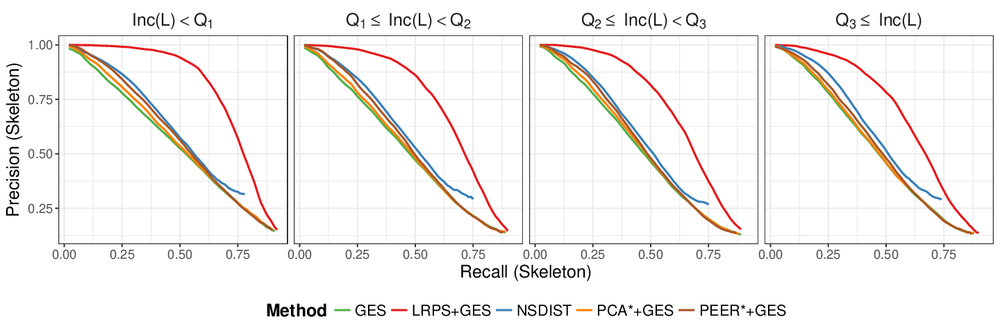
In our second set of simulations, we draw from a more diverse set of hidden structures. We set but draw and uniformly at random from and respectively. We generate 500 datasets according to this scheme. In order to quantify the departure of from our assumptions we compute , the incoherence of , for each of the 500 datasets (the distribution of along with figures showing the effect of are shown in the appendix). In this second scenario, many datasets explicitly violate our assumptions since there are many hidden variables acting in a sparse fashion.
In Figure 2 b), we plot average precision/recall curves for this second simulation design. The datasets are divided into four bins based on the quartiles of ’s distribution (noted ), so that the leftmost panel corresponds to the 125 datasets for which it is easiest to estimate . Doing so indicates how our approach is expected to behave in the most adverse scenarios. As can be seen from this figure, LRpS+GES outperforms other approaches in terms of skeleton recovery.
5.2. Total Causal Effect Estimation
Under our assumptions is the causal DAG so that the Markov equivalence class encoded by contains the causal DAG. For any given pair of distinct nodes , we can therefore estimate the total causal effect of on for all DAGs in the Markov equivalence class. Since one of these DAGs is the true causal DAG, this yields a list of possible total causal effects which includes the true total causal effect. The IDA approach makes it possible to generate such lists efficiently without enumerating all DAGs in the Markov equivalence class [34, 32]. The original IDA method described in Maathuis et al. [34] uses the PC algorithm in order to first estimate a CPDAG, and then computes sets of possible total causal effects using the sample covariance matrix and the output of the first stage. However, it is possible to replace this first step by any other algorithm which estimates a CPDAG. Likewise, any estimator of can replace .
Since LRPS+GES outputs a CPDAG, we can assess its ability to estimate total causal effects by using it in the first stage of IDA. Thus, lists of possible causal effects are generated using the estimated CPDAG and the covariance matrix . We denote this method by (LRPS+GES),IDA. For all pairs , , we compute the set of possible total causal effects of on . Pairs of variables are then ranked according to . This ranking is compared to the true total causal effects using the precision and recall metrics, e.g. “precision at rank ” would be the number of pairs that are in the top pairs and have a non-zero total causal effect in the true DAG, divided by .
In this section, we select a single DAG, PAG or CPDAG along the regularisation paths in order to apply IDA or LV-IDA. Thus, we pick a value of the tuning parameters for both the first and second stages. This is in contrast with the previous section where only the tuning parameters of the first stages (when applicable) were selected, while we reported precision-recall curves for the whole regularisation paths of the second stages. We consider the following methods, where the first stage tuning parameters are selected as before (when applicable):
- :
-
GES,IDA: the CPDAG is estimated using GES. The tuning parameter is chosen with the BIC. IDA is applied with the resulting CPDAG and the sample covariance matrix .
- :
-
NSDIST,IDA: the DAG is estimated using NSDIST and converted to a CPDAG. The tuning parameter for the second stage (, with the notations of [21]) is chosen using the BIC. IDA is applied with the resulting CPDAG and the sample covariance matrix .
- :
-
(PCA*+GES*),IDA: the top principal components are first estimated from the data and regressed out. The CPDAG is estimated using GES on the residuals. The tuning parameter is chosen with perfect knowledge so as to maximise the average precision (in terms of causal effect recovery). IDA is applied with the resulting CPDAG and the covariance matrix of the residuals.
- :
-
(LRpS+GES),IDA: the CPDAG is estimated using LRpS+GES. The tuning parameter of the second stage is chosen with the BIC. IDA is applied with the resulting CPDAG and the covariance matrix .
- :
-
RFCI,LV-IDA [11, 35]: the PAG is estimated with RFCI. The significance level for RFCI is given by 44 4 In a number of cases, the LV-IDA algorithm, when applied to a single dataset, was still running after a few days of computation. Given that we simulated data from hundreds of datasets, we could not experiment with many values of .. LV-IDA is applied to the resulting PAG and the sample covariance matrix . Whenever LV-IDA outputs an NA, the corresponding pair is not counted, i.e. it is neither a true positive nor false positive.
- :
-
RANDOM,IDA: one hundred random DAGs are generated from the same model as was used in the simulation. Total causal effects are then estimated based on the resulting CPDAG and the sample covariance matrix . We report the interval spanned by the 2.5-97.5 percentiles of the distribution of precisions at fixed recalls.
- :
-
EMPTY, IDA: Causal effects are computed without adjustment, which is equivalent to applying the ida function of the pcalg package to an empty graph and the sample covariance matrix.
With respect to total causal effect estimation, we found (PEER*+GES*),IDA and (PCA* + GES*),IDA to be nearly undistinguishable, which is why PEER is not reported here. Moreover, note that since we are reporting results for the GES,IDA approach, we are not considering the “PC,IDA” method. Indeed, GES has been shown to have good finite sample performance, and recent high-dimensional consistency guarantees have been given in Nandy et al. [37].
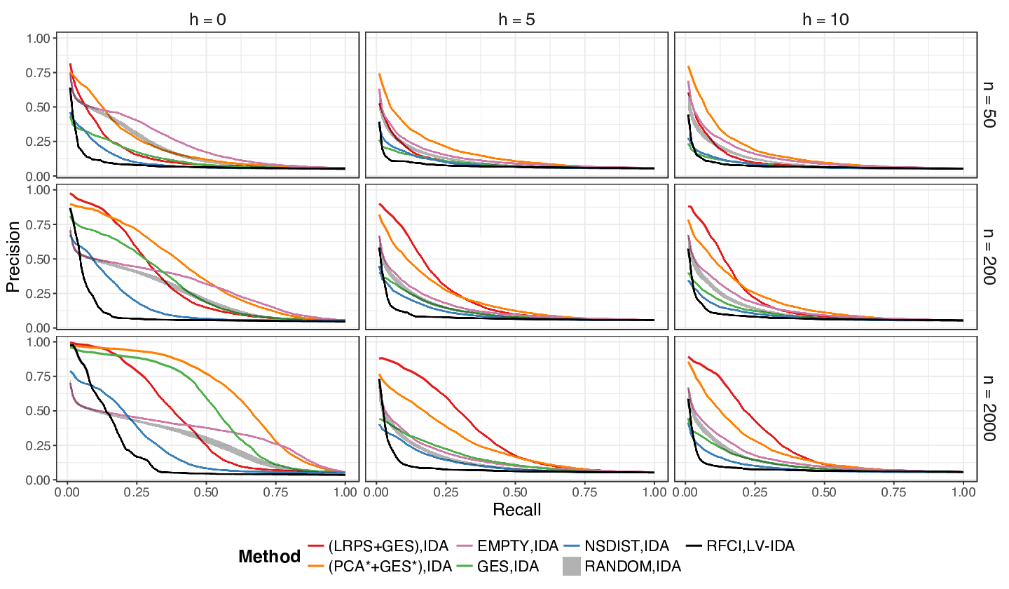
We consider the same simulation designs as in the previous section. Figure 3 a) displays the results obtained in the first setting, the one where hidden variables are influential. Unlike in Figure 2, the orientation of the directed edges matters. When the sample size is relatively small , there appear to be little to gain from using (CP)DAG estimation methods – the EMPTY approach is competitive. As soon as the sample size increases and , there is a clear benefit in using LRpS+GES. When , LRpS+GES is outperformed but its performances remain comparable to those of GES. Since it is designed to handle hidden variables, the behaviour of RFCI,LV-IDA might come as a surprise. First, we see that when there is no confounding, RFCI,LV-IDA is capable of achieving a high precision. This is consistent with previous findings indicating that LV-IDA is conservative but capable of recovering a small but high-quality set of total causal effects [35]. When , the set of models we simulate from is particularly challenging for methods relying on MAGs since nearly all pairs of observed variables are confounded. It is therefore not surprising to see RFCI,LV-IDA being outperformed.
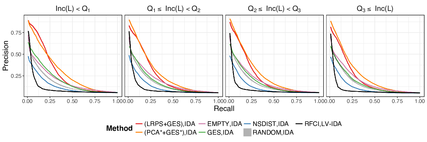
As can be seen from Figure 3 b), LRpS+GES performs at least as well other approaches and, in most cases, it performs better. As pointed out above, it is in the most challenging scenarios, when confounders act in a sparse fashion (rightmost panel), that RFCI,LV-IDA is the most useful. It is very conservative but is capable of achieving the highest precision.
Finally, we recall that for the (PCA*+GES*),IDA method, both the number of principal components to regress out and the tuning parameter for GES are chosen so as to maximise the area under the precision/recall curves. This provides a benchmark for the method, but such performances could not be achieved on a real dataset. This explains the discrepancy between (PCA*+GES*),IDA and GES,IDA when : GES,IDA selects using the BIC. It also puts into perspective the performances of (LRpS+GES),IDA and RFCI,LV-IDA, which are sometimes far better than the other approaches in spite of selecting the tuning parameters from the data only.
a)
b)
5.3. Hubs, Robustness to Outliers and Non-Linearities
In our simulations, we considered situations when the assumption on does not hold, i.e. when the hidden variables are not impacting a large fraction of the observed variables, but act in a sparse fashion instead. Additionally, one can wonder what happens when the conditions on are not met, i.e. the DAG over observed variables is not so sparse and it has a high degree. In the supplementary materials, we simulate random graphs from the Barabasi model and report results showing to what extent our approach is affected by such graphs with hubs. A summary of our findings is that LRpS+GES is indeed outperformed by GES when there are hubs with a high degree and no hidden variables. When the hubs are of moderate size and there are hidden confounders, LRpS+GES remains superior to PEER and clearly outperforms GES. Finally, when hubs have a high degree and there are latent variables, the performance of all methods is degraded, but LRpS+GES is less affected than its counterparts.
We also looked at the performances of the Kendall-LRpS+GES estimator described in Algorithm 3.2 by simulating data contaminated with samples drawn from a Cauchy distribution (a violation of our condition on ) and marginally transformed by strictly increasing functions (), or non-monotonic functions () – another violation of our assumptions. We found Kendall-LRPS+GES to be especially robust to outliers, even in the presence of hidden variables. When variables are marginally transformed with a non monotonic function, all methods are impacted, but methods based on rank correlations remain far superior. All results and further details are available in the supplementary materials.
6. Applications
6.1. Application 1: Isoprenoid Synthesis in Arabidopsis thaliana
We illustrate a few properties of our approach on a dataset containing gene expression measurements taken in Arabidopsis thaliana grown under different conditions (such as light/darkness, growth hormones, etc…) [55]. [55] gave particular attention to the genes involved in isoprenoid synthesis. In Arabidopsis thaliana, two pathways, located in distinct organs, are responsible for isoprenoid synthesis: the mevalonate pathway (MVA) and the non-mevalonate pathway (MEP). We downloaded the data made available in the supplementary materials of [55] and took the genes represented in Figure 3 of [55]. They fall into three categories: genes that are part of the MVA pathway, genes that are in the MEP pathway and mitochondrial genes. For illustration, Figure 4 a) shows the adjacency matrix of the metabolic pathways. This is a graph in which nodes are genes and edges are chemical reactions between gene products. This graph, while related to the regulatory network we aim to estimate, is very different from it: in general, both the structure and the direction of the edges differ. However, it gives information about which genes are in which pathways.
We fitted LRpS and Kendall-LRpS to our data and selected the tuning parameters and with five-fold cross-validation. The low-rank matrix estimated by LRpS had two non-zero eigenvalues, with ratio . Hence, only the first eigenvector was retained. In order to see whether we could interpret the hidden variables estimated by LRpS, we looked at the loadings of the genes in the first eigenvector of . Figure 4 b) shows the distribution of the loadings per pathway and suggests that the main source of variation in the data is given by these pathways, which are sometimes unknown in less studied organisms. By applying GES to – the inverse of the sparse output of LRpS – we are therefore modelling a regulatory network conditionally on those pathways, without having to provide further information. Similar results were obtained with Kendal-LRpS+GES and are plotted in the appendix.
a)
b)

In Figures 5 a) and b), we show the adjacency matrices of the CPDAGs obtained by running GES and LRpS+GES using the BIC score for GES. Figure 5 c) shows the adjacency matrix of the PAG obtained by RFCI, with as before. In Figures 5 d), e), the matrices of total causal effects computed from GES,IDA and (LRPS+GES),IDA are plotted, where IDA is used as in our simulations. In Figure 5 f), the output of LV-IDA is plotted, with NAs marked in red. The graphs and total causal effects obtained from other methods (NSDIST,IDA, etc…) are plotted in the appendix. The output of Kendall-LRpS+GES is also shown in the appendix and differs from LRpS+GES in that there are more circle marks and slightly fewer edges. Qualitatively, it yields results that are similar to LRpS+GES. Figure 5 illustrates the tendency of LV-IDA to produce very conservative estimates of the causal effects, with many pairs being either zero or NA. On the other extreme, the causal effects of GES are stronger than those of LRpS+GES. In particular, LRpS+GES does not find any strong causal relationship between mitochondrial genes and any other genes, as indicated by the “white cross” in the middle of the matrix plotted in Figure 5 e). Both GES and LRpS+GES support the hypothesis of cross-talk from the MEP to the MVA pathway.
a)
b)

c)
d)
e)

f)
The metabolic pathways of Arabidopsis thaliana have been studied in detail but, to the best of our knowledge, no reliable ground-truth is available for its directed regulatory network. For that reason, it is difficult to assess the quality of the estimated CPDAGs or matrices of total causal effects. Nonetheless, we were able to show that the various methods can yield very different results and to qualitatively assess them. This application also gave us the opportunity to compare LV-IDA to other IDA-based methods on a real dataset.
6.2. Application 2: Regulatory Network in Ovarian Cancer
We now consider the problem of identifying the targets regulated by a given set of transcription factors in a human gene expression dataset. This problem is often considered in the literature because it constitutes an example of a real-life dataset for which the existence and direction of some edges is known, thus making it possible to compare estimated graphs to a “partial ground-truth” [51, 21]. Briefly, a transcription factor is a protein which regulates the mRNA expression of a gene by binding to a specific DNA sequence near its promoting region. Some families of transcription factors have been studied in detail, and publicly available databases such as TRRUST provide lists of transcription factors along with the genes – called targets – they regulate [20]. transcription factors play a crucial in role in cancer development, which is why it is believed that intervening on the expression of such genes could alter the course of some cancers [12].
In this application, we follow closely the steps described in Section 5.1 of [21] where ovarian adenocarcinomas are studied. We used the RNA-Seq data available from the National Cancer Institute (portal.gdc.cancer.gov/) and log-transformed the gene expression levels. There is a consensus about how important some transcription factor families are for cancer development [12, 42]. We therefore selected the transcription factors belonging to those families55 5 Namely: FOS, FOSB, JUN, JUNB, JUND, ESR1, ESR2, AR, NFKB1, NFKB2, RELA, RELB, REL, STAT1, STAT2, STAT3, STAT4, STAT5, STAT6. Following [21], we also extracted the genes that are known to have direct interactions with these transcription factors according to NetBox66 6 http://sanderlab.org/tools/netbox.html, “a software tool for performing network analysis on human interaction networks which is pre-loaded with networks derived from four curated data sources, including the Human Protein Reference Database (HPRD), Reactome, NCI-Nature Pathway Interaction (PID) Database, and the MSKCC Cancer Cell Map”. The resulting dataset contained genes and samples.
To construct a reference network to which we can compare our estimates, we used the output of NetBox. NetBox outputs a list of known (unoriented) interactions between some of the 501 selected genes. Unfortunately, nothing indicates whether those interactions are causal; in general it is not because two genes interact in NetBox that intervening on the expression levels of one of the genes will induce a change in the expression level of the other. However, thanks to our knowledge of transcription factors, we do know that whenever there is an interaction between a transcription factor and a non-transcription factor, then it is likely to be causal and directed from the transcription factor to its target. Moreover, transcription factors are tissue specific, meaning that we can only expect a subset of the interactions to be active in any given cell-type [14]. These observations allow us to build three reference networks: a) an undirected graph in which there is an edge between A and B whenever they are said to interact according to NetBox (this is Network A); b) a “causal” undirected graph in which only edges between transcription factors and their targets have been retained (Network B); c) a causal directed graph in which the edges of Network B have been ordered from transcription factors to their targets (Network C).
In this application, the number of variables () is rather large compared to the sample size (). We therefore selected the tuning parameters of LRpS () using the Extended BIC instead of cross-validation [16].
In Figure 6 we compare the output of various methods (GES, LRpS+GES, NSDIST, PCA*+GES, PEER*+GES) to reference networks A, B and C in terms of True and False Positive Rates (TPR, FPR). For Network C, we follow again [21]: an undirected edge in a CPDAG is counted as half a true positive and half a false negative. In grey, we plot the range spanned by the 2.5 and 97.5 percentiles of our null distribution. It was computed by first picking 100 random ordering of the variables and, starting from a complete DAG, removing random edges one after the other until there are no edges left. After each removal, we computed the performance metrics of the DAG with respect to all reference networks, thus generating 100 random regularisation paths for each of the plots.
Figure 6 a) plots the Receiving Operator Curve (ROC) for Network A. All methods display comparable performances, although NSDIST and LRpS+GES appear slightly above GES. In Figure 6 b), we restrict ourselves to Network B, so that only transcription factor-target edges are counted. LRpS+GES is clearly above NSDIST, PCA*+GES and PEER*+GES which are themselves outperforming GES. When the direction of the edges is also taken into account (Figure 6 c)), LRpS+GES remains ahead of the other methods, and NSDIST beats PCA and PEER. The difference in performance between NSDIST and GES does not come as a surprise since Figure 6 a) and b) reproduce the findings of Figures 4 a) and b) of [21].
a)

b)

c)

d)

Since NetBox is not restricted to transcription factor-target interactions, we sought to confirm the results of Figure 6 c) by using an independent source of validation specialised in transcriptional regulatory relationships. We used TRRUST [20] and constructed Network D by adding directed edges between transcription factors and targets according to TRRUST. In Figure 6 d) we plot the resulting ROC cuve, which reproduces the results obtained using NetBox transcription factor-target interactions as ground truth.
Making definitive statements about the nature of the hidden confounders in this dataset is difficult. We can hypothesise that it is prone to the type of confounding typically seen in gene expression data where intersample heterogeneities (e.g. relatedness, batch effects) are often responsible for unwanted variations. Gaining access to the patients’ DNA would make it possible to test whether relatedness between samples is indeed a cause of confounding in our dataset. Batch effects can also be accounted for to some extent, but there will always remain confounders that cannot be ruled out. For example, it has been observed that factors as varied as the time postportem a sample is collected, or the ozone levels in the laboratory introduce spurious correlations [27].
It is also possible that unobserved transcriptions factors, or transcription factors that are not in our database, are responsible for these gene-gene interactions. This highlights one of the limitations of our method.
7. Discussion
We discussed the problem of estimating the Markov equivalence class of a DAG in the presence of hidden variables. Building on previous work by [6] and [8], we suggested a two-stage approach – termed LRpS+GES – which first removes unwanted variation using latent Gaussian graphical model selection, and then estimates a CPDAG by applying GES. We chose GES for its good empirical performance and theoretical guarantees [37], but we note that the second step can be replaced by any structure learning algorithm for DAGs that assumes causal sufficiency -- although another choice might not offer the same theoretical guarantees. Our main theoretical result states that LRpS+GES is consistent for CPDAG recovery in some sparse high-dimensional regimes. Through simulations and two applications to gene expression datasets, we showed that our approach often outperforms the state of the art, both in terms of graphical structure recovery and total causal effect estimation. Moreover, the results reported in our simulations can be achieved in practice since tuning parameter selection was performed using in-sample information only77 7 The code for our simulations and applications is made available with this paper..
When it comes to removing unwanted variation from biological datasets, state-of-the-art approaches usually incorporate external information into the analysis by including additional covariates (e.g. gender, genetic relatedness), thus also accounting for known confounders [49, 36]. Since these additional covariates are often discrete, modelling them with LRpS+GES would be a violation of our assumptions. In such a setting, it is straightforward to replace LRpS by the LSCGGM estimator suggested in [17]. LSCGGM makes it possible to perform a low rank plus sparse decomposition, conditionally on a number of arbitrarily distributed random variables. The LRpS+GES approach could therefore be replaced by the “LSCGGM+GES” estimator, which would come with similar theoretical guarantees.
The computational cost of LRpS+GES might also be a concern to the practitioner. In Algorithm 3.1 we first estimate an inverse covariance matrix . To the best of our knowledge, the fastest algorithm for this LRpS step uses the so-called alternative direction method of multipliers, with a cost of per iteration [31]. Next, must be inverted, at a cost of , and then GES is run on . For large problems, this last step can be replaced by the ARGES algorithm suggested in Nandy et al. [37].
As detailed earlier, there exist other approaches which are capable of estimating DAG models and total causal effects in the presence of hidden variables, i.e. FCI-type algorithms [47, 11, 9] and LV-IDA [35]. In both our simulations and our first application, we found that such approaches are very conservative under our assumptions. However, they do outperform LRpS+GES when hidden variables act on the observed ones in a sparse fashion. As such, LRpS+GES is complementary to existing methods.
Finally, we note that the LRpS+GES estimator can be modified to tackle another widespread problem: selection bias. Reusing the notations introduced in Section 3.1, selection bias can be handled as follows. Let be a zero-mean random vector which follows a multivariate normal distribution with covariance matrix . Let us further assume that there exists a DAG, say, which is a perfect map of the distribution . Then, assuming that the variables in are selection variables, we only see observations from
By the Woodbury identity, this can be rewritten in terms of the precision matrix as
where is a negative semi-definite matrix defined as
Since Theorem 4.1 of [6] does not make any assumptions about the positive-definitiveness of , the following estimator could replace LRpS in the first stage of LRpS+GES:
| (13) |
where and . This modified approach is consistent in the presence of selection variables under the similar conditions as Theorem 4.1. The only difference is in the interpretation of the condition , which would require that be sparse and that there be few selection variables that are directly regulated by many of the observed variables.
Acknowledgements
We are grateful to Wu Jun for numerous insightful comments on our proofs and software. We are also indebted to the anonymous reviewers for their suggestions on how to expand to the scope of our paper and for pointing out some inconsistencies. Their advice brought about significant changes from which the present work benefited greatly.
References
- [1] Aguet, F. et al. (2016) Local genetic effects on gene expression across 44 human tissues. Tech. rep. Available at http://dx.doi.org/10.1101/074450.
- [2] Ali, R. A., Richardson, T. S. and Spirtes, P. (2009) Markov equivalence for ancestral graphs. Ann. Statist., 37, 2808–2837.
- [3] Andersson, S. A., Madigan, D. and Perlman, M. D. (1997) A characterization of Markov equivalence classes for acyclic digraphs. Ann. Statist., 25, 505–541.
- [4] Bollen, K. (1989) Structural equations with latent variables.
- [5] Candès, E. J., Li, X., Ma, Y. and Wright, J. (2011) Robust principal component analysis? J. ACM, 58, Art. 11.
- [6] Chandrasekaran, V., Parrilo, P. A. and Willsky, A. S. (2012) Latent variable graphical model selection via convex optimization. Ann. Statist., 40, 1935–1967.
- [7] Chandrasekaran, V., Sanghavi, S., Parrilo, P. A. and Willsky, A. S. (2011) Rank-sparsity incoherence for matrix decomposition. SIAM Journal on Optimization, 21, 572–596.
- [8] Chickering, D. M. (2002) Learning equivalence classes of Bayesian-network structures. J. Mach. Learn. Res., 2, 445–498.
- [9] Claassen, T., Mooij, J. M. and Heskes, T. (2013) Learning sparse causal models is not NP-hard. In Proceedings of the Twenty-Ninth Conference on Uncertainty in Artificial Intelligence, UAI’13, 172–181.
- [10] Colombo, D. and Maathuis, M. (2014) Order-independent constraint-based causal structure learning. J. Mach. Learn. Res., 15, 3741–3782.
- [11] Colombo, D., Maathuis, M. H., Kalisch, M. and Richardson, T. S. (2012) Learning high-dimensional directed acyclic graphs with latent and selection variables. Ann. Statist., 40, 294–321.
- [12] Darnell, J. E. (2002) Transcription factors as targets for cancer therapy. Nature Reviews Cancer, 2, 740–749.
- [13] Drton, M. and Maathuis, M. H. (2017) Structure learning in graphical modeling. Annual Review of Statistics and Its Application, 4, 365–393.
- [14] Eeckhoute, J., Métivier, R. and Salbert, G. (2009) Defining specificity of transcription factor regulatory activities. Journal of Cell Science, 122, 4027–4034.
- [15] Fang, K., Kotz, S. and Ng, K. (1990) Symmetric multivariate and related distributions. Monographs on statistics and applied probability. Chapman and Hall.
- [16] Foygel, R. and Drton, M. (2010) Extended bayesian information criteria for Gaussian graphical models. In Advances in Neural Information Processing Systems 23, 604–612.
- [17] Frot, B., Jostins, L. and McVean, G. (2018) Graphical model selection for Gaussian conditional random fields in the presence of latent variables. Journal of the American Statistical Association. To Appear.
- [18] Gagnon-Bartsch, J. A., Jacob, L. and Speed, T. P. (2013) Removing unwanted variation from high dimensional data with negative controls. Tech. Rep. 820, Department of Statistics, University of California at Berkeley.
- [19] Han, F. and Liu, H. (2017) Statistical analysis of latent generalized correlation matrix estimation in transelliptical distribution. Bernoulli, 23, 23–57.
- [20] Han, H., Shim, H., Shin, D., Shim, J. E., Ko, Y., Shin, J., Kim, H., Cho, A., Kim, E., Lee, T., Kim, H., Kim, K., Yang, S., Bae, D., Yun, A., Kim, S., Kim, C. Y., Cho, H. J., Kang, B., Shin, S. and Lee, I. (2015) TRRUST: a reference database of human transcriptional regulatory interactions. Scientific Reports, 5.
- [21] Han, S. W., Chen, G., Cheon, M.-S. and Zhong, H. (2016) Estimation of directed acyclic graphs through two-stage adaptive lasso for gene network inference. J. Am. Statist. Ass., 111, 1004–1019.
- [22] Harris, N. and Drton, M. (2013) PC algorithm for nonparanormal graphical models. J. Mach. Learn. Res., 14, 3365–3383.
- [23] Hastie, T., Tibshirani, R. and Wainwright, M. (2015) Statistical Learning with Sparsity: The Lasso and Generalizations. Boca Raton, USA: Chapman & Hall/CRC.
- [24] Heinze-Deml, C., Maathuis, M. H. and Meinshausen, N. (2018) Causal structure learning. Annual Review of Statistics and Its Application, 5.
- [25] Kalisch, M. and Bühlmann, P. (2007) Estimating high-dimensional directed acyclic graphs with the PC-algorithm. J. Mach. Learn. Res., 8, 613–636.
- [26] Kalisch, M., Mächler, M., Colombo, D., Maathuis, M. and Bühlmann, P. (2012) Causal inference using graphical models with the R package pcalg. J. Statist. Software, 47, 1–26.
- [27] Kang, H. M., Ye, C. and Eskin, E. (2008) Accurate discovery of expression quantitative trait loci under confounding from spurious and genuine regulatory hotspots. Genetics, 180, 1909–1925. URL: http://www.genetics.org/content/180/4/1909.
- [28] Lauritzen, S. L. (1996) Graphical models, vol. 17 of Oxford Statistical Science Series. New York: The Clarendon Press Oxford University Press.
- [29] Leek, J. T. and Storey, J. D. (2007) Capturing heterogeneity in gene expression studies by surrogate variable analysis. PLoS Genetics, 3, e161.
- [30] Liu, H., Han, F. and Zhang, C.-h. (2012) Transelliptical graphical models. In Proceedings of the 25th International Conference on Neural Information Processing Systems 21, 800–808. Curran Associates Inc.
- [31] Ma, S., Xue, L. and Zou, H. (2013) Alternating direction methods for latent variable gaussian graphical model selection. Neural Comput., 25, 2172–2198.
- [32] Maathuis, M. H., Colombo, D., Kalisch, M. and Bühlmann, P. (2010a) Predicting causal effects in large-scale systems from observational data. Nature methods, 7, 247–8.
- [33] Maathuis, M. H., Colombo, D., Kalisch, M. and Bühlmann, P. (2010b) Predicting causal effects in large-scale systems from observational data. Nat. Methods, 7, 247–248.
- [34] Maathuis, M. H., Kalisch, M. and Bühlmann, P. (2009) Estimating high-dimensional intervention effects from observational data. Ann. Statist., 37, 3133–3164.
- [35] Malinsky, D. and Spirtes, P. (2017) Estimating bounds on causal effects in high-dimensional and possibly confounded systems. International Journal of Approximate Reasoning, 88, 371 – 384.
- [36] Mostafavi, S., Battle, A., Zhu, X., Urban, A. E., Levinson, D., Montgomery, S. B. and Koller, D. (2013) Normalizing RNA-sequencing data by modeling hidden covariates with prior knowledge. PLoS ONE, 8, e68141.
- [37] Nandy, P., Hauser, A. and Maathuis, M. H. (2017a) High-dimensional consistency in score-based and hybrid structure learning. Available at: arXiv:1507.02608.
- [38] Nandy, P., Maathuis, M. H. and Richardson, T. S. (2017b) Estimating the effect of joint interventions from observational data in sparse high-dimensional settings. Ann. Statist., 45, 647–674.
- [39] Pearl, J. (2009a) Causal inference in statstics: an overview. Statistics Surveys, 3, 96–146.
- [40] — (2009b) Causality: Models, Reasoning and Inference. Cambridge: Cambridge University Press, 2nd edn.
- [41] Qi, H. and Sun, D. (2006) A quadratically convergent newton method for computing the nearest correlation matrix. SIAM J. Matrix Anal. Appl, 28, 2006.
- [42] Redell, M. and Tweardy, D. (2005) Targeting transcription factors for cancer therapy. Current Pharmaceutical Design, 11, 2873–2887.
- [43] Richardson, T. S. and Spirtes, P. (2002) Ancestral graph Markov models. Ann. Statist., 30, 962–1030.
- [44] Robinson, R. W. (1977) Counting unlabeled acyclic digraphs, 28–43. Combinatorial Mathematics V: Proceedings of the Fifth Australian Conference. Springer Berlin Heidelberg.
- [45] Silva, R., Scheines, R., Glymour, C. and Spirtes, P. (2006) Learning the structure of linear latent variable models. J. Mach. Learn. Res., 7, 191–246.
- [46] Spirtes, P., Glymour, C. and Scheines, R. (2000) Causation, Prediction, and Search. Adaptive Computation and Machine Learning. Cambridge: MIT Press, second edn.
- [47] Spirtes, P., Meek, C. and Richardson, T. (1995) Causal inference in the presence of latent variables and selection bias. In In Proceedings of Eleventh Conference on Uncertainty in Artificial Intelligence, 499–506. San Francisco, CA: Morgan Kaufmann.
- [48] Spirtes, P., Richardson, T., Meek, C., Scheines, R. and Glymour, C. (1998) Using path diagrams as a structural equation modeling tool. Sociological Methods & Research, 27, 182–225.
- [49] Stegle, O., Parts, L., Piipari, M., Winn, J. and Durbin, R. (2012) Using probabilistic estimation of expression residuals (PEER) to obtain increased power and interpretability of gene expression analyses. Nature Protocols, 7, 500–507.
- [50] Taeb, A., Reager, J. T., Turmon, M. and Chandrasekaran, V. (2017) A statistical graphical model of the california reservoir system. Water Resources Research, 53, 9721–9739.
- [51] Tsamardinos, I., Brown, L. E. and Aliferis, C. F. (2006) The max-min hill-climbing Bayesian network structure learning algorithm. Mach. Learn., 65, 31–78.
- [52] Verma, T. and Pearl, J. (1991) Equivalence and synthesis of causal models. In Proceedings of the Sixth Annual Conference on Uncertainty in Artificial Intelligence, UAI ’90, 255–270. New York, NY, USA: Elsevier Science Inc.
- [53] Vershynin, R. (2012) Introduction to the non-asymptotic analysis of random matrices. In Compressed Sensing: Theory and Applications, 210–268. Cambridge Univ Press. Available at http://www-personal.umich.edu/ romanv/papers/non-asymptotic-rmt-plain.pdf.
- [54] Wegkamp, M. and Zhao, Y. (2016) Adaptive estimation of the copula correlation matrix for semiparametric elliptical copulas. Bernoulli, 22, 1184–1226.
- [55] Wille, A., Zimmermann, P., Vranová, E., Fürholz, A., Laule, O., Bleuler, S., Hennig, L., Prelić, A., von Rohr, P., Thiele, L., Zitzler, E., Gruissem, W. and Bühlmann, P. (2004) Sparse graphical Gaussian modeling of the isoprenoid gene network in arabidopsis thaliana. Genome Biology, 5, R92.
- [56] Zhang, J. (2008) On the completeness of orientation rules for causal discovery in the presence of latent confounders and selection bias. Artificial Intelligence, 172, 1873–1896.
- [57] Zou, H. (2006) The adaptive lasso and its oracle properties. J. Am. Statist. Ass., 101, 1418–1429.