跳到论文正文
W Papers独立论文阅读器 arXiv:1708.00465 论文正文 计算阅读时间 · 0%
引用这篇论文根据当前论文元数据生成,正式投稿前建议核对。


License: arXiv.org perpetual non-exclusive license
arXiv:1708.00465v1 [math.NA] 01 Aug 2017

Intrinsic Frequency Analysis and Fast Algorithms

Peyman Tavallali1,∗, Hana Koorehdavoudi2, Joanna Krupa3
Abstract.

Intrinsic Frequency (IF) has recently been introduced as an ample signal processing method for analyzing carotid and aortic pulse pressure tracings. The IF method has also been introduced as an effective approach for the analysis of cardiovascular system dynamics. The physiological significance, convergence and accuracy of the IF algorithm has been established in prior works. In this paper, we show that the IF method could be derived by appropriate mathematical approximations from the Navier-Stokes and elasticity equations. We further introduce a fast algorithm for the IF method based on the mathematical analysis of this method. In particular, we demonstrate that the IF algorithm can be made faster, by a factor or more than 100 times, using a proper set of initial guesses based on the topology of the problem, fast analytical solution at each point iteration, and substituting the brute force algorithm with a pattern search method. Statistically, we observe that the algorithm presented in this article complies well with its brute-force counterpart. Furthermore, we will show that on a real dataset, the fast IF method can draw correlations between the extracted intrinsic frequency features and the infusion of certain drugs. In general, this paper aims at a mathematical analysis of the IF method to show its possible origins and also to present faster algorithms.

1Division of Engineering and Applied Sciences, California Institute of Technology, 1200 East California Boulevard, MC 205-45, Pasadena, CA 91125, USA

2Aerospace and Mechanical Engineering, University of Southern California, Los Angeles, CA 90089-1453, USA

3Avicena LLC, 2400 N Lincoln Ave, Altadena, CA 91001, USA

∗Corresponding Author, email: ptavalla@caltech.edu, tavallali@gmail.com

1. Introduction

Cardiovascular diseases (CVDs) and stroke are major causes of death in the United States. The total cost related to CVDs and stroke was estimated to be more than $316 billion in 2011-2012 [20, 22]. Hence, clinical measurements of cardiovascular health indices are of great importance. These methods and measurements are essential tools for monitoring cardiovascular health due to their relative availability. For example, Left Ventricular Ejection Fraction (LVEF) is a measure of left ventricular contractility [6] and Carotid-Femoral Pulse Wave Velocity (cfPWV) is a measure of aortic stiffness [18].

However, current methods of measuring such indices are expensive, sometimes invasive, prone to measurement errors, and not necessarily easy to use. For example, 2D LVEF echocardiography is not accurate compared to more expensive and laborious gold standard cardiac MRI method [10, 12, 15, 14]. As another example, obtaining accurate cfPWV measurements often requires certain medical devices and a well-trained staff within a clinical setting [29]. Consequently, continuous measurement of these indices is not practical. These limitations emphasize the need for new cardiovascular monitoring methods.

Intrinsic Frequency (IF) has been established as a new method of cardiovascular monitoring through a novel signal processing methodology [26]. The IF method needs only an uncalibrated pulse pressure [31] to extract pertinent information regarding the cardiovascular health of an individual [26]. The IF method has also been shown to be capable of non-invasively measuring LVEF by means of an iPhone camera [25]. We believe that methods like IF are of clinical and financial benefit in addressing cardiovascular monitoring.

In this paper, at first, we provide an overview of the IF method. Next, we present an approximate derivation of the IF model by combining Navier-Stokes equations and continuity with elasticity equations. This helps to build a solid mathematical foundation for the IF method and the analysis that follows. Later, we analyze the IF algorithm in the space of feasible solutions, and based on that, we introduce a new version of the IF algorithm which is faster than the current brute-force IF method [31] while maintaining the same accuracy. We then perform a case study on real pressure waveforms drawn from canine data using our new algorithm. We will see that the fast IF algorithm is capable of capturing the effects of different drug infusions on a canine subject.

2. Brief Overview of IF method

2.1. A History of Analyzing Cardiovascular Pulse Waveform

Blood pressure was first measured by Hales in 1735 [13]. In his measurements, he found that blood pressure is not constant in the arterial system. He related these variations to the elasticity of the arteries [13]. Currently, it is known that the shape of the arterial pulse wave is intimately related to the physiology and pathology of the whole arterial system [1]. There has been much research on analyzing the dynamics of blood pressure and flow in arterial systems [2, 9, 23, 24, 33]. Specifically, there are two main approaches to analyzing cardiovascular pulse wave data. One approach is based on a systematic mathematical framework for the cardiovascular system. The other is based on directly analyzing the pulse pressure waveform using signal processing methods.

An example of the systematic framework can be seen with the set of Windkessel models [34]. The formulation of a minimal lumped model of the arterial system was first presented by Westerhof et al. [34]. Based on a Windkessel model, the arterial system dynamics have been modeled through a combination of different elements such as resistance, compliance and impedance. In this simplified model of the arterial system, the blood flow dynamics is modeled by the interaction between the elements (assuming the blood flow acts as the current in the system). Because of the type of modeling, the wave transmission of the blood flow is neglected. As a result, the Windkessel models is not able to represent the entire dynamics of the blood flow in an arterial system accurately.

On the other hand, there are various methods for direct analysis of an arterial pulse waveform, in both time and frequency domains [24]. For example, the impedance method, which is based on Fourier transform, is a common method to analyze the pressure waveform in the frequency domain [2]. As an example, Milnor has shown that the pressure and flow waveforms can be a superposition of several harmonics using the Fourier method [21]. Another method to investigate the pressure wave in the time domain is the wave intensity analysis which is based on wavelet transform [8]. These methods do not necessarily convey a physical understanding of the cardiovascular system.

The IF algorithm presented in [31] is analyzing a pulse waveform through a direct time-frequency signal processing machinery setting, from a quantitative perspective. Although, in previous work [26], we tried to qualitatively express a systems approach to the IF formulation, the quantitative picture has not yet been clear. However, in this article, we show this connection from a quantitative perspective.

2.2. IF Formulation

In the IF method, the aortic pressure waveform at time t∈[0,T)t\in\left[0,T\right), for a cardiac period TT, can be represented as

(2.1) S⁡(ai,bi,p¯,ωi,t)=(a1cosω1t+b1sinω1t+p¯)𝟏[0,T0)(t)+(a2cosω2t+b2sinω2t+p¯)𝟏[T0,T)(t),\begin{array}[]{ccc}S\left(a_{i},b_{i},\bar{p},\omega_{i};t\right)&=&\left(a_{1}\cos\omega_{1}t+b_{1}\sin\omega_{1}t+\bar{p}\right)\mathbf{1}_{\left[0,T_{0}\right)}\left(t\right)+\\ &&\left(a_{2}\cos\omega_{2}t+b_{2}\sin\omega_{2}t+\bar{p}\right)\mathbf{1}_{\left[T_{0},T\right)}\left(t\right),\end{array}

with a continuity condition at T0T_{0} and periodicity at TT. In this formulation, the indicator function is defined as

𝟏[x,y)​(t)={1,x≤t<y,0,e​l​s​e.\mathbf{1}_{\left[x,y\right)}\left(t\right)=\left\{\begin{array}[]{cc}1,&x\leq t<y,\\ 0,&else.\end{array}\right.

Here, a1a_{1}, b1b_{1}, a2a_{2} and b2b_{2} are the envelopes of the IF model fit. ω1\omega_{1} and ω2\omega_{2} are the Intrinsic Frequencies (IFs) of the waveform. Further, p¯\bar{p} is the mean pressure during the cardiac cycle. This type of formulation embeds the coupling and decoupling of heart and aorta.

The goal of the IF model (2.1) is to extract a fit, called Intrinsic Mode Function (IMF), that carries most of the energy (information) from an observed pressure waveform f⁡(t)f\left(t\right) in one period. The latter is done by solving the following optimization problem [31]:

(2.2) m​i​n​i​m​i​z​eai,bi,ωi,p¯‖f⁡(t)−S⁡(ai,bi,p¯,ωi,t)‖22\begin{array}[]{cc}\underset{a_{i},b_{i},\omega_{i},\bar{p}}{minimize}&\left\|f\left(t\right)-S\left(a_{i},b_{i},\bar{p},\omega_{i};t\right)\right\|_{2}^{2}\end{array}
(2.3) s​u​b​j​e​c​t​t​o​a1cosω1T0+b1sinω1T0=a2cosω2T0+b2sinω2T0,a1=a2cosω2T+b2sinω2T.subject\,to\begin{array}[]{ccc}a_{1}\cos\omega_{1}T_{0}+b_{1}\sin\omega_{1}T_{0}&=&a_{2}\cos\omega_{2}T_{0}+b_{2}\sin\omega_{2}T_{0},\\ a_{1}&=&a_{2}\cos\omega_{2}T+b_{2}\sin\omega_{2}T.\end{array}

Here, ‖‖2\left\|\right\|_{2} is the L2L^{2}-norm. The first linear condition in this optimization enforces the continuity of the extracted IMF at the dicrotic notch. The second one imposes the periodicity. The mathematical convergence and accuracy of the IF algorithm have been explained in a previous work [31]. In the next sections, we explore the foundation of the IF algorithm and propose a faster IF algorithm.

3. Approximate Derivation of the IF Model

As mentioned earlier, in a previous work [26], we tried to express a systems approach to the IF formulation qualitatively. However, in this article, we show this connection from a quantitative perspective. This section is devoted to this purpose.

In this paper, we assume that the Left Ventricle (LV), the aortic valve, aorta and the arterial system can be represented by a simplified model as shown in Figure 1. Here, the LV and the aortic valve are assumed to be the boundary condition at the entrance of the aortic tube and the arterial system is the terminal boundary condition of the aortic tube. The boundary condition at the entrance of the aortic tube changes from an LV boundary condition to a closed valve boundary condition, at the dicrotic notch time T0T_{0} during a cardiac cycle [0,T]\left[0,T\right]. We further assume that blood is a Newtonian incompressible fluid, the aorta is a straight and sufficiently long elastic tube with a constant circular cross section and there is no external force causing flow rotation. These assumptions are not all satisfied in a real cardiovascular system. However, they are useful in estimating the general behavior of blood in aorta.

Combining the Navier-Stokes equations and continuity with the elasticity equation, we can drive a model for the flow Q⁡(x,t)Q\left(x,t\right) and the pressure P⁡(x,t)P\left(x,t\right) along the length xx of an aorta as follow

(3.1) −∂P∂x​(x,t)=L​∂Q∂t​(x,t)+R​Q​(x,t),-\frac{\partial P}{\partial x}\left(x,t\right)=L\frac{\partial Q}{\partial t}\left(x,t\right)+RQ\left(x,t\right),
(3.2) −∂Q∂x​(x,t)=C​∂P∂t​(x,t).-\frac{\partial Q}{\partial x}\left(x,t\right)=C\frac{\partial P}{\partial t}\left(x,t\right).

The step by step derivation of these equations is presented in Appendix A. Parameters LL, RR, and CC represent inductance, resistance, and compliance of the blood in aorta. Here, 0≤x≤h0\leq x\leq h, where hh represents the aortic length. This model has also been discussed and simulated numerically in [3] with a complex set of boundary conditions. Here, our main concentration will be on the aortic tube oscillatory waveform solutions. Next, we will show that we can derive (2.1) from (3.1) and (3.2).

Since the input to the IF model (2.1) is a pressure waveform, we need to extract an equation for the pressure P⁡(x,t)P\left(x,t\right) from Equations (3.1) and (3.2) by eliminating the flow. Combining Equations (3.1) and (3.2) results in

(3.3) C​L​∂2P∂t2​(x,t)+C​R​∂P∂t​(x,t)=∂2P∂x2​(x,t).CL\frac{\partial^{2}P}{\partial t^{2}}\left(x,t\right)+CR\frac{\partial P}{\partial t}\left(x,t\right)=\frac{\partial^{2}P}{\partial x^{2}}\left(x,t\right).

Taking P⁡(x,t)=𝒦⁡(t)​p​(x,t)+p¯P\left(x,t\right)=\mathcal{K}\left(t\right)p\left(x,t\right)+\bar{p}, with p¯\bar{p} as the the mean pressure, we can write equation (3.3) as

(3.4) (C​L​𝒦¨​(t)+C​R​𝒦˙​(t))​p​(x,t)+(2​C​L​𝒦˙​(t)+C​R​𝒦​(t))​∂p∂t​(x,t)+C​L​𝒦​(t)​∂2p∂t2​(x,t)=𝒦⁡(t)​∂2p∂x2​(x,t).\begin{array}[]{c}\left(CL\ddot{\mathcal{K}}\left(t\right)+CR\dot{\mathcal{K}}\left(t\right)\right)p\left(x,t\right)+\left(2CL\dot{\mathcal{K}}\left(t\right)+CR\mathcal{K}\left(t\right)\right)\frac{\partial p}{\partial t}\left(x,t\right)+CL\mathcal{K}\left(t\right)\frac{\partial^{2}p}{\partial t^{2}}\left(x,t\right)\\ =\mathcal{K}\left(t\right)\frac{\partial^{2}p}{\partial x^{2}}\left(x,t\right).\end{array}

Here, we have used the dot notation to represent the time derivative. We can simplify the term in front of ∂p∂t​(x,t)\frac{\partial p}{\partial t}\left(x,t\right), in (3.4), by setting 2​C​L​𝒦˙​(t)+C​R​𝒦​(t)=02CL\dot{\mathcal{K}}\left(t\right)+CR\mathcal{K}\left(t\right)=0. The latter has a solution 𝒦⁡(t)=K​e−R2​L​t\mathcal{K}\left(t\right)=Ke^{-\frac{R}{2L}t} for some constant KK. This reduces Equation (3.4) into

(3.5) C​L​∂2p∂t2​(x,t)−C​R24​L​p​(x,t)=∂2p∂x2​(x,t).CL\frac{\partial^{2}p}{\partial t^{2}}\left(x,t\right)-\frac{CR^{2}}{4L}p\left(x,t\right)=\frac{\partial^{2}p}{\partial x^{2}}\left(x,t\right).

The solution of Equation (3.5) can be expressed in terms of eigenfunctions. In other words, using the method of separation of the variables, one can express the solution of Equation (3.5) as

(3.6) p⁡(x,t)=∑n=1∞Tn​(t)​Xn​(x)p\left(x,t\right)=\sum_{n=1}^{\infty}T_{n}\left(t\right)X_{n}\left(x\right)

for

(3.7) Tn​(t)=αn​s​i​n​(ωn​t)+βn​c​o​s​(ωn​t),T_{n}\left(t\right)=\mathcal{\alpha}_{n}sin\left(\omega_{n}t\right)+\beta_{n}cos\left(\omega_{n}t\right),
(3.8) Xn​(x)=ζn​s​i​n​(C​L​(ωn)2−C​R24​L​x)+ηn​c​o​s​(C​L​(ωn)2−C​R24​L​x),X_{n}\left(x\right)=\zeta_{n}sin\left(\sqrt{CL\left(\omega_{n}\right)^{2}-\frac{CR^{2}}{4L}}x\right)+\eta_{n}cos\left(\sqrt{CL\left(\omega_{n}\right)^{2}-\frac{CR^{2}}{4L}}x\right),

and some constants αn\mathcal{\alpha}_{n}, βn\beta_{n}, ζn\zeta_{n} and ηn\eta_{n}. As a result, the solution of (3.3) can be expressed as

(3.9) P(x,t)=p¯+Ke−R2​L​t∑n=1∞{(αnsin(ωnt)+βncos(ωnt))(ζnsin(C​L​(ωn)2−C​R24​Lx)+ηncos(C​L​(ωn)2−C​R24​Lx))}.\begin{array}[]{c}P\left(x,t\right)=\bar{p}+Ke^{-\frac{R}{2L}t}\sum_{n=1}^{\infty}\Biggl\{\left(\mathcal{\alpha}_{n}sin\left(\omega_{n}t\right)+\beta_{n}cos\left(\omega_{n}t\right)\right)\\ \left(\zeta_{n}sin\left(\sqrt{CL\left(\omega_{n}\right)^{2}-\frac{CR^{2}}{4L}}x\right)+\eta_{n}cos\left(\sqrt{CL\left(\omega_{n}\right)^{2}-\frac{CR^{2}}{4L}}x\right)\right)\Biggr\}.\end{array}

The variables ωn\omega_{n} can be expressed based on the boundary conditions of the aortic tube. We need to emphasize that for a period of the cardiac cycle [0,T)\left[0,T\right), the boundary conditions change before and after the dicrotic notch T0T_{0}. Hence, for t∈[0,T)t\in\left[0,T\right), Equation (3.9) can be written as

(3.10) P⁡(x,t)=p¯+𝟏[0,T0)(t)K1e−R2​L​t∑n=1∞{(αn1sin(ωn1t)+βn1cos(ωn1t))(ζn1sin(C​L​(ωn1)2−C​R24​Lx)+ηn1cos(C​L​(ωn1)2−C​R24​Lx))}+𝟏[T0,T)(t)K2e−R2​L​t∑n=1∞{(αn2sin(ωn2t)+βn2cos(ωn2t))(ζn2sin(C​L​(ωn2)2−C​R24​Lx)+ηn2cos(C​L​(ωn2)2−C​R24​Lx))}.\begin{array}[]{c}P\left(x,t\right)=\bar{p}\\ +\mathbf{1}_{\left[0,T_{0}\right)}\left(t\right)K^{1}e^{-\frac{R}{2L}t}\sum_{n=1}^{\infty}\Biggl\{\left(\mathcal{\alpha}_{n}^{1}sin\left(\omega_{n}^{1}t\right)+\beta_{n}^{1}cos\left(\omega_{n}^{1}t\right)\right)\\ \left(\zeta_{n}^{1}sin\left(\sqrt{CL\left(\omega_{n}^{1}\right)^{2}-\frac{CR^{2}}{4L}}x\right)+\eta_{n}^{1}cos\left(\sqrt{CL\left(\omega_{n}^{1}\right)^{2}-\frac{CR^{2}}{4L}}x\right)\right)\Biggr\}\\ +\mathbf{1}_{\left[T_{0},T\right)}\left(t\right)K^{2}e^{-\frac{R}{2L}t}\sum_{n=1}^{\infty}\Biggl\{\left(\mathcal{\alpha}_{n}^{2}sin\left(\omega_{n}^{2}t\right)+\beta_{n}^{2}cos\left(\omega_{n}^{2}t\right)\right)\\ \left(\zeta_{n}^{2}sin\left(\sqrt{CL\left(\omega_{n}^{2}\right)^{2}-\frac{CR^{2}}{4L}}x\right)+\eta_{n}^{2}cos\left(\sqrt{CL\left(\omega_{n}^{2}\right)^{2}-\frac{CR^{2}}{4L}}x\right)\right)\Biggr\}.\end{array}

Here, the superscripts indicated with “1” belong to the form of the solution before the closure of the aortic valve, and the superscripts indicated with “2” belong to the form of the solution after the closure of the aortic valve. Constants K1K^{1}, αn1\alpha{}_{n}^{1}, βn1\beta{}_{n}^{1}, ζn1\zeta{}_{n}^{1}, ηn1\eta{}_{n}^{1} and ωn1\omega{}_{n}^{1} are found from the boundary and initial conditions at systole. Similarly, constants K2K^{2}, αn2\alpha{}_{n}^{2}, βn2\beta{}_{n}^{2}, ζn2\zeta{}_{n}^{2}, ηn2\eta{}_{n}^{2} and ωn2\omega{}_{n}^{2} are found from the boundary and initial conditions at diastole.

Equation (3.10) is explicitly showing the coupling and decoupling of heart and aorta before and after the dicrotic notch. As the boundary conditions change during a cardiac cycle, the frequencies of oscillation also change from ωn1\omega_{n}^{1} to ωn2\omega_{n}^{2}. Generally, Equation (3.9) can represent pressure waveform for a Newtonian incompressible fluid in a straight and sufficiently long elastic tube with constant circular cross section.

If the pressure is recorded at a specific point x0x_{0} on aorta, the terms containing the spacial variable xx would be fixed. In other words, Equation (3.10) would reduce to

(3.11) P⁡(x=x0,t)=p¯+{K1​e−R2​L​t​∑n=1∞κn1​(αn1​s​i​n​(ωn1​t)+βn1​c​o​s​(ωn1​t))}​𝟏[0,T0)​(t)+{K2​e−R2​L​t​∑n=1∞κn2​(αn2​s​i​n​(ωn2​t)+βn2​c​o​s​(ωn2​t))}​𝟏[T0,T)​(t),\begin{array}[]{c}P\left(x=x_{0},t\right)=\bar{p}\\ +\left\{K^{1}e^{-\frac{R}{2L}t}\sum_{n=1}^{\infty}\kappa_{n}^{1}\left(\mathcal{\alpha}_{n}^{1}sin\left(\omega_{n}^{1}t\right)+\beta_{n}^{1}cos\left(\omega_{n}^{1}t\right)\right)\right\}\mathbf{1}_{\left[0,T_{0}\right)}\left(t\right)\\ +\left\{K^{2}e^{-\frac{R}{2L}t}\sum_{n=1}^{\infty}\kappa_{n}^{2}\left(\mathcal{\alpha}_{n}^{2}sin\left(\omega_{n}^{2}t\right)+\beta_{n}^{2}cos\left(\omega_{n}^{2}t\right)\right)\right\}\mathbf{1}_{\left[T_{0},T\right)}\left(t\right),\end{array}

for

κn1=ζn1​s​i​n​(C​L​(ωn1)2−C​R24​L​x0)+ηn1​c​o​s​(C​L​(ωn1)2−C​R24​L​x0)\kappa_{n}^{1}=\zeta_{n}^{1}sin\left(\sqrt{CL\left(\omega_{n}^{1}\right)^{2}-\frac{CR^{2}}{4L}}x_{0}\right)+\eta_{n}^{1}cos\left(\sqrt{CL\left(\omega_{n}^{1}\right)^{2}-\frac{CR^{2}}{4L}}x_{0}\right)

and

κn2=ζn2​s​i​n​(C​L​(ωn2)2−C​R24​L​x0)+ηn2​c​o​s​(C​L​(ωn2)2−C​R24​L​x0).\kappa_{n}^{2}=\zeta_{n}^{2}sin\left(\sqrt{CL\left(\omega_{n}^{2}\right)^{2}-\frac{CR^{2}}{4L}}x_{0}\right)+\eta_{n}^{2}cos\left(\sqrt{CL\left(\omega_{n}^{2}\right)^{2}-\frac{CR^{2}}{4L}}x_{0}\right).

Now, considering that the cardiac cycle length would be around 1.5​s​e​c1.5\,sec, at most, and taking into account that RR is smaller than LL [3], one can use the approximation e−R2​L​t≃1e^{-\frac{R}{2L}t}\simeq 1. Hence, Equation (3.11) would become

(3.12) P⁡(x=x0,t)≈p¯+{K1​∑n=1∞κn1​(αn1​s​i​n​(ωn1​t)+βn1​c​o​s​(ωn1​t))}​𝟏[0,T0)​(t)+{K2​∑n=1∞κn2​(αn2​s​i​n​(ωn2​t)+βn2​c​o​s​(ωn2​t))}​𝟏[T0,T)​(t).\begin{array}[]{c}P\left(x=x_{0},t\right)\approx\bar{p}\\ +\left\{K^{1}\sum_{n=1}^{\infty}\kappa_{n}^{1}\left(\mathcal{\alpha}_{n}^{1}sin\left(\omega_{n}^{1}t\right)+\beta_{n}^{1}cos\left(\omega_{n}^{1}t\right)\right)\right\}\mathbf{1}_{\left[0,T_{0}\right)}\left(t\right)\\ +\left\{K^{2}\sum_{n=1}^{\infty}\kappa_{n}^{2}\left(\mathcal{\alpha}_{n}^{2}sin\left(\omega_{n}^{2}t\right)+\beta_{n}^{2}cos\left(\omega_{n}^{2}t\right)\right)\right\}\mathbf{1}_{\left[T_{0},T\right)}\left(t\right).\end{array}

Further, if most of the information, or energy, is carried out by the first terms in the series of the solution, we can further write the approximated solution (3.12) as

(3.13) P⁡(x=x0,t)≈p¯+{K1​κ11​(α11​s​i​n​(ω11​t)+β11​c​o​s​(ω11​t))}​𝟏[0,T0)​(t)+{K2​κ12​(α12​s​i​n​(ω12​t)+β12​c​o​s​(ω12​t))}​𝟏[T0,T)​(t).\begin{array}[]{c}P\left(x=x_{0},t\right)\approx\bar{p}\\ +\left\{K^{1}\kappa_{1}^{1}\left(\mathcal{\alpha}_{1}^{1}sin\left(\omega_{1}^{1}t\right)+\beta_{1}^{1}cos\left(\omega_{1}^{1}t\right)\right)\right\}\mathbf{1}_{\left[0,T_{0}\right)}\left(t\right)\\ +\left\{K^{2}\kappa_{1}^{2}\left(\mathcal{\alpha}_{1}^{2}sin\left(\omega_{1}^{2}t\right)+\beta_{1}^{2}cos\left(\omega_{1}^{2}t\right)\right)\right\}\mathbf{1}_{\left[T_{0},T\right)}\left(t\right).\end{array}

Now, by relabeling

(3.14) b1=K1​κ11​α11,b_{1}=K^{1}\kappa_{1}^{1}\mathcal{\alpha}_{1}^{1},
(3.15) a1=K1​κ11​β11,a_{1}=K^{1}\kappa_{1}^{1}\beta_{1}^{1},
(3.16) b2=K2​κ12​α12,b_{2}=K^{2}\kappa_{1}^{2}\mathcal{\alpha}_{1}^{2},
(3.17) a2=K2​κ12​β12,a_{2}=K^{2}\kappa_{1}^{2}\beta_{1}^{2},
(3.18) ω1=ω11,\omega_{1}=\omega_{1}^{1},
(3.19) ω2=ω12,\omega_{2}=\omega_{1}^{2},

we can approximate the IF model (2.1). The continuity and periodicity conditions (2.3) can also be approximated if we hold the assumption that most of the energy is carried out by the first terms in the series of the solution (3.12).

In short, in this section, we have presented an approximate quantitative justification on the origins of the IF method. In the next section, we move on with the analysis of the optimization problem (2.2) subject to (2.3).

4. Analysis of The IF Algorithm

Practically, one must solve the discrete version of (2.2). We assume that the pressure waveform f⁡(t)f\left(t\right) is sampled uniformly. Also, we can simplify (2.2) by the fact that any sinusoid can be assumed to start from time t=0t=0 with a compensation coming from a phase shift. In other words, any sinusoid can be expressed as A​cos⁡ω​t+B​sin⁡ω​tA\cos\omega t+B\sin\omega t, irrespective of whether the initial time is t=0t=0 or t=T0t=T_{0}. Hence, the discrete format of (2.2) can be expressed as

(4.1) m​i​n​i​m​i​z​eai,bi,ωi,p¯‖𝐟−𝐒⁡(ai,bi,p¯,ωi,𝐭)‖22s​u​b​j​e​c​t​t​oa1cosω1T0+b1sinω1T0=a2,a1=a2cosω2(T−T0)+b2sinω2(T−T0),\begin{array}[]{cc}\underset{a_{i},b_{i},\omega_{i},\bar{p}}{minimize}&\left\|\mathbf{f}-\mathbf{S}\left(a_{i},b_{i},\bar{p},\omega_{i};\mathbf{t}\right)\right\|_{2}^{2}\\ \\ subject\,to&\begin{array}[]{ccc}a_{1}\cos\omega_{1}T_{0}+b_{1}\sin\omega_{1}T_{0}&=&a_{2}\phantom{\cos\omega_{2}\left(T-T_{0}\right)+b_{2}\sin\omega_{2}\left(T-T_{0}\right)},\\ a_{1}&=&a_{2}\cos\omega_{2}\left(T-T_{0}\right)+b_{2}\sin\omega_{2}\left(T-T_{0}\right),\end{array}\end{array}

for 𝐟=(f1,…,fn+m)′\mathbf{f}=\left(f_{1},\ldots,f_{n+m}\right)^{\prime} as the uniform sampling of the original cycle. Here, by taking

(4.2) 𝐭=(𝐭1′,𝐭2′)′=(t11,t12,…,t1n,t21,t22,…,t2m)′∈ℝ(n+m)×1\mathbf{t}=\left(\mathbf{t}_{1}^{\prime},\mathbf{t}_{2}^{\prime}\right)^{\prime}=\left(t_{1}^{1},t_{1}^{2},\ldots,t_{1}^{n},t_{2}^{1},t_{2}^{2},\ldots,t_{2}^{m}\right)^{\prime}\in\mathbb{R}^{\left(n+m\right)\times 1}

for 𝐭1=(0,Δ​t,2​Δ​t,…,T0)′∈ℝn×1\mathbf{t}_{1}=\left(0,\Delta t,2\Delta t,\ldots,T_{0}\right)^{\prime}\in\mathbb{R}^{n\times 1} and 𝐭2=(Δ​t,2​Δ​t,…,T−T0)′∈ℝm×1\mathbf{t}_{2}=\left(\Delta t,2\Delta t,\ldots,T-T_{0}\right)^{\prime}\in\mathbb{R}^{m\times 1}, we have the discrete form of S⁡(ai,bi,p¯,ωi,t)S\left(a_{i},b_{i},\bar{p},\omega_{i};t\right) as

(4.3) 𝐒⁡(ai,bi,p¯,ωi,𝐭)=(a1cosω1𝐭1+b1sinω1𝐭1a2cosω2𝐭2+b2sinω2𝐭2)+p¯​𝟏.\mathbf{S}\left(a_{i},b_{i},\bar{p},\omega_{i};\mathbf{t}\right)=\left(\begin{array}[]{c}a_{1}\cos\omega_{1}\mathbf{t}_{1}+b_{1}\sin\omega_{1}\mathbf{t}_{1}\\ a_{2}\cos\omega_{2}\mathbf{t}_{2}+b_{2}\sin\omega_{2}\mathbf{t}_{2}\end{array}\right)+\bar{p}\mathbf{1}.

In this article, (.)′\left(.\right)^{\prime} denotes the transpose operator and the vector 𝟏=(1,1,…,1)′∈ℝ(n+m)×1\mathbf{1}=\left(1,1,\ldots,1\right)^{\prime}\in\mathbb{R}^{\left(n+m\right)\times 1}. Also,

(4.4) cos⁡ω1​𝐭1=(cos⁡ω1​t11,…,cos⁡ω1​t1n)′,sin⁡ω1​𝐭1=(sin⁡ω1​t11,…,sin⁡ω1​t1n)′,cos⁡ω2​𝐭2=(cos⁡ω2​t21,…,cos⁡ω2​t2m)′,sin⁡ω2​𝐭2=(sin⁡ω2​t21,…,sin⁡ω2​t2m)′.\begin{array}[]{c}\cos\omega_{1}\mathbf{t}_{1}=\left(\cos\omega_{1}t_{1}^{1},\ldots,\cos\omega_{1}t_{1}^{n}\right)^{\prime},\\ \sin\omega_{1}\mathbf{t}_{1}=\left(\sin\omega_{1}t_{1}^{1},\ldots,\sin\omega_{1}t_{1}^{n}\right)^{\prime},\\ \cos\omega_{2}\mathbf{t}_{2}=\left(\cos\omega_{2}t_{2}^{1},\ldots,\cos\omega_{2}t_{2}^{m}\right)^{\prime},\\ \sin\omega_{2}\mathbf{t}_{2}=\left(\sin\omega_{2}t_{2}^{1},\ldots,\sin\omega_{2}t_{2}^{m}\right)^{\prime}.\end{array}

The constraints, in (4.1), can be written as

(4.5) (cos⁡ω1​T0−1sin⁡ω1​T001−cos⁡ω2​(T−T0)0−sin⁡ω2​(T−T0))​(a1a2b1b2)=(00).\left(\begin{array}[]{cccc}\cos\omega_{1}T_{0}&-1&\sin\omega_{1}T_{0}&0\\ 1&-\cos\omega_{2}\left(T-T_{0}\right)&0&-\sin\omega_{2}\left(T-T_{0}\right)\end{array}\right)\left(\begin{array}[]{c}a_{1}\\ a_{2}\\ b_{1}\\ b_{2}\end{array}\right)=\left(\begin{array}[]{c}0\\ 0\end{array}\right).

If we can solve for two, out of four, unknowns in (4.5), we would make (4.1) an unconstrained optimization. However, it is important to check whether the matrix in (4.5) is of full rank or not. In fact, the rows of this matrix are linearly independent except when

(4.6) cosω1T0cosω2(T−T0)=1.\cos\omega_{1}T_{0}\cos\omega_{2}\left(T-T_{0}\right)=1.

This will lead into two cases:

  1. (1)

    Degenerate Case in which Equation (4.6) holds,

  2. (2)

    General Case in which, it does not.

4.1. General Case (cosω1T0cosω2(T−T0)≠1\cos\omega_{1}T_{0}\cos\omega_{2}\left(T-T_{0}\right)\neq 1)

One can solve the constraints in (4.1) for a1a_{1} and a2a_{2} to obtain

(4.7) a1=b1sinω1T0cosω2(T−T0)+b2sinω2(T−T0)1−cosω1T0cosω2(T−T0),a_{1}=\frac{b_{1}\sin\omega_{1}T_{0}\cos\omega_{2}\left(T-T_{0}\right)+b_{2}\sin\omega_{2}\left(T-T_{0}\right)}{1-\cos\omega_{1}T_{0}\cos\omega_{2}\left(T-T_{0}\right)},
(4.8) a2=b1sinω1T0+b2cosω1T0sinω2(T−T0)1−cosω1T0cosω2(T−T0).a_{2}=\frac{b_{1}\sin\omega_{1}T_{0}+b_{2}\cos\omega_{1}T_{0}\sin\omega_{2}\left(T-T_{0}\right)}{1-\cos\omega_{1}T_{0}\cos\omega_{2}\left(T-T_{0}\right)}.

Equations (4.7) and (4.8) would then simplify (4.3) into

(4.9) 𝐒⁡(ω1,ω1,b1,b2,p¯,𝐭)=𝐐⁡(ω1,ω1,b1,b2,𝐭)+p¯​𝟏,\mathbf{S}\left(\omega_{1},\omega_{1},b_{1},b_{2},\bar{p};\mathbf{t}\right)=\mathbf{Q}\left(\omega_{1},\omega_{1},b_{1},b_{2};\mathbf{t}\right)+\bar{p}\mathbf{1},

where 𝐐⁡(ω1,ω1,b1,b2,𝐭)=b1​𝐯1​(ω1,ω2,𝐭)+b2​𝐯2​(ω1,ω2,𝐭)\mathbf{Q}\left(\omega_{1},\omega_{1},b_{1},b_{2};\mathbf{t}\right)=b_{1}\mathbf{v}_{1}\left(\omega_{1},\omega_{2};\mathbf{t}\right)+b_{2}\mathbf{v}_{2}\left(\omega_{1},\omega_{2};\mathbf{t}\right) for

(4.10) 𝐯1​(ω1,ω2,𝐭)=(sinω1T0cosω2(T−T0)1−cosω1T0cosω2(T−T0)cosω1𝐭1+sinω1𝐭1sin⁡ω1​T01−cosω1T0cosω2(T−T0)cosω2𝐭2),\mathbf{v}_{1}\left(\omega_{1},\omega_{2};\mathbf{t}\right)=\left(\begin{array}[]{c}\frac{\sin\omega_{1}T_{0}\cos\omega_{2}\left(T-T_{0}\right)}{1-\cos\omega_{1}T_{0}\cos\omega_{2}\left(T-T_{0}\right)}\cos\omega_{1}\mathbf{t}_{1}+\sin\omega_{1}\mathbf{t}_{1}\\ \frac{\sin\omega_{1}T_{0}}{1-\cos\omega_{1}T_{0}\cos\omega_{2}\left(T-T_{0}\right)}\cos\omega_{2}\mathbf{t}_{2}\end{array}\right),

and

(4.11) 𝐯2​(ω1,ω2,𝐭)=(sin⁡ω2​(T−T0)1−cosω1T0cosω2(T−T0)cosω1𝐭1cosω1T0sinω2(T−T0)1−cosω1T0cosω2(T−T0)cosω2𝐭2+sinω2𝐭2).\mathbf{v}_{2}\left(\omega_{1},\omega_{2};\mathbf{t}\right)=\left(\begin{array}[]{c}\frac{\sin\omega_{2}\left(T-T_{0}\right)}{1-\cos\omega_{1}T_{0}\cos\omega_{2}\left(T-T_{0}\right)}\cos\omega_{1}\mathbf{t}_{1}\\ \frac{\cos\omega_{1}T_{0}\sin\omega_{2}\left(T-T_{0}\right)}{1-\cos\omega_{1}T_{0}\cos\omega_{2}\left(T-T_{0}\right)}\cos\omega_{2}\mathbf{t}_{2}+\sin\omega_{2}\mathbf{t}_{2}\end{array}\right).

Using Equations (4.9)-(4.11), and dropping the dependencies in notation, simplifies (4.1) into

(4.12) m​i​n​i​m​i​z​eω1,ω2,b1,b2,p¯​‖𝐐+p¯​𝟏−𝐟‖22.\underset{\omega_{1},\omega_{2},b_{1},b_{2},\bar{p}}{minimize}\,\left\|\mathbf{Q}+\bar{p}\mathbf{1}-\mathbf{f}\right\|_{2}^{2}.

This simplification has helped to eliminate the constraints in the optimization problem (4.1).

The minimization problem (4.12) is non-convex and non-linear in its parameters. So, in order to be able to solve the problem, we can use the fact that the minimum of a function can first be found over some variables and then over the remaining ones [7]. In other words, the optimization problem in (4.12) can be written as

(4.13) m​i​n​i​m​i​z​eω1,ω2​(m​i​n​i​m​i​z​eb1,b2,p¯​‖𝐐+p¯​𝟏−𝐟‖22).\underset{\omega_{1},\omega_{2}}{minimize}\,\left(\underset{b_{1},b_{2},\bar{p}}{minimize}\,\left\|\mathbf{Q}+\bar{p}\mathbf{1}-\mathbf{f}\right\|_{2}^{2}\right).

We call the inner optimization in (4.13) as P⁡(ω1,ω2)P\left(\omega_{1},\omega_{2}\right). Solving for P⁡(ω1,ω2)P\left(\omega_{1},\omega_{2}\right) is a classical least squares problem. The solution existence and uniqueness of this optimization is mentioned in our previous work [31]. To find the exact solution we simplify the objective function as

(4.14) ‖𝐐+p¯​𝟏−𝐟‖22=(𝐐+p¯​𝟏−𝐟)′​(𝐐+p¯​𝟏−𝐟)=𝐐′​𝐐+2​p¯​𝐐′​𝟏−2​𝐐′​𝐟−2​p¯​𝐟′​𝟏+p¯​𝟏′​𝟏+𝐟′​𝐟.\begin{array}[]{cc}\left\|\mathbf{Q}+\bar{p}\mathbf{1}-\mathbf{f}\right\|_{2}^{2}=&\left(\mathbf{Q}+\bar{p}\mathbf{1}-\mathbf{f}\right)^{\prime}\left(\mathbf{Q}+\bar{p}\mathbf{1}-\mathbf{f}\right)\\ \phantom{\left\|\mathbf{Q}+\bar{p}\mathbf{1}-\mathbf{f}\right\|_{2}^{2}}=&\mathbf{Q}^{\prime}\mathbf{Q}+2\bar{p}\mathbf{Q}^{\prime}\mathbf{1}-2\mathbf{Q}^{\prime}\mathbf{f}-2\bar{p}\mathbf{f}^{\prime}\mathbf{1}+\bar{p}\mathbf{1}^{\prime}\mathbf{1}+\mathbf{f}^{\prime}\mathbf{f}.\end{array}

Substituting for 𝐐=b1​𝐯1+b2​𝐯2\mathbf{Q}=b_{1}\mathbf{v}_{1}+b_{2}\mathbf{v}_{2}, we convert (4.14) into

(4.15) ‖𝐐+p¯​𝟏−𝐟‖22=b12​𝐯1′​𝐯1+2​b1​b2​𝐯1′​𝐯2+b22​𝐯2′​𝐯2+2​p¯​b1​𝐯1′​𝟏+2​p¯​b2​𝐯2′​𝟏−2​b1​𝐯1′​𝐟−2​b2​𝐯2′​𝐟−2​p¯​𝐟′​𝟏+p¯2​𝟏′​𝟏+𝐟′​𝐟.\begin{array}[]{cc}\left\|\mathbf{Q}+\bar{p}\mathbf{1}-\mathbf{f}\right\|_{2}^{2}=&b_{1}^{2}\mathbf{v}_{1}^{\prime}\mathbf{v}_{1}+2b_{1}b_{2}\mathbf{v}_{1}^{\prime}\mathbf{v}_{2}+b_{2}^{2}\mathbf{v}_{2}^{\prime}\mathbf{v}_{2}+2\bar{p}b_{1}\mathbf{v}_{1}^{\prime}\mathbf{1}+2\bar{p}b_{2}\mathbf{v}_{2}^{\prime}\mathbf{1}\\ &-2b_{1}\mathbf{v}_{1}^{\prime}\mathbf{f}-2b_{2}\mathbf{v}_{2}^{\prime}\mathbf{f}-2\bar{p}\mathbf{f}^{\prime}\mathbf{1}+\bar{p}^{2}\mathbf{1}^{\prime}\mathbf{1}+\mathbf{f}^{\prime}\mathbf{f}.\end{array}

Since, in this part of the optimization, the values of ω1\omega_{1} and ω2\omega_{2} are fixed, we can find the optimal values of b1b_{1}, b2b_{2}, and p¯\bar{p} by setting the partial derivatives of (4.15) equal to zero. In other words, we set ∂(‖𝐐+p¯​𝟏−𝐟‖22)∂b1=0\frac{\partial\left(\left\|\mathbf{Q}+\bar{p}\mathbf{1}-\mathbf{f}\right\|_{2}^{2}\right)}{\partial b_{1}}=0, ∂(‖𝐐+p¯​𝟏−𝐟‖22)∂b2=0\frac{\partial\left(\left\|\mathbf{Q}+\bar{p}\mathbf{1}-\mathbf{f}\right\|_{2}^{2}\right)}{\partial b_{2}}=0, and ∂(‖𝐐+p¯​𝟏−𝐟‖22)∂p¯=0\frac{\partial\left(\left\|\mathbf{Q}+\bar{p}\mathbf{1}-\mathbf{f}\right\|_{2}^{2}\right)}{\partial\bar{p}}=0. Doing this, we find the optimal solution for b1b_{1}, b2b_{2}, and p¯\bar{p}, by

(4.16) (b1∗​(ω1,ω2)b2∗​(ω1,ω2)p¯∗​(ω1,ω2))=(𝐯1′​𝐯1𝐯1′​𝐯2𝐯1′​𝟏𝐯1′​𝐯2𝐯2′​𝐯2𝐯2′​𝟏𝐯1′​𝟏𝐯2′​𝟏𝟏′​𝟏)−1​(𝐯1′​𝐟𝐯2′​𝐟𝟏′​𝐟).\left(\begin{array}[]{c}b_{1}^{*}\left(\omega_{1},\omega_{2}\right)\\ b_{2}^{*}\left(\omega_{1},\omega_{2}\right)\\ \bar{p}^{*}\left(\omega_{1},\omega_{2}\right)\end{array}\right)=\left(\begin{array}[]{ccc}\mathbf{v}_{1}^{\prime}\mathbf{v}_{1}&\mathbf{v}_{1}^{\prime}\mathbf{v}_{2}&\mathbf{v}_{1}^{\prime}\mathbf{1}\\ \mathbf{v}_{1}^{\prime}\mathbf{v}_{2}&\mathbf{v}_{2}^{\prime}\mathbf{v}_{2}&\mathbf{v}_{2}^{\prime}\mathbf{1}\\ \mathbf{v}_{1}^{\prime}\mathbf{1}&\mathbf{v}_{2}^{\prime}\mathbf{1}&\mathbf{1}^{\prime}\mathbf{1}\end{array}\right)^{-1}\left(\begin{array}[]{c}\mathbf{v}_{1}^{\prime}\mathbf{f}\\ \mathbf{v}_{2}^{\prime}\mathbf{f}\\ \mathbf{1}^{\prime}\mathbf{f}\end{array}\right).

Here, we have fulfilled the optimization part by solving a linear system. This could potentially accelerate the IF algorithm. Finally, we only have to solve a minimization on

(4.17) P⁡(ω1,ω2)=‖𝐐⁡(ω1,ω2,b1∗​(ω1,ω2),b2∗​(ω1,ω2),𝐭)+p¯∗​(ω1,ω2)​𝟏−𝐟‖22,P\left(\omega_{1},\omega_{2}\right)=\left\|\mathbf{Q}\left(\omega_{1},\omega_{2},b_{1}^{*}\left(\omega_{1},\omega_{2}\right),b_{2}^{*}\left(\omega_{1},\omega_{2}\right);\mathbf{t}\right)+\bar{p}^{*}\left(\omega_{1},\omega_{2}\right)\mathbf{1}-\mathbf{f}\right\|_{2}^{2},

which is

(4.18) m​i​n​i​m​i​z​eω1,ω2​P​(ω1,ω2).\underset{\omega_{1},\omega_{2}}{minimize}\,P\left(\omega_{1},\omega_{2}\right).

We note that a property of the function P⁡(ω1,ω2)P\left(\omega_{1},\omega_{2}\right) is its differentiability, away from its singularities. In fact, by definition, the function ‖𝐐+p¯​𝟏−𝐟‖22\left\|\mathbf{Q}+\bar{p}\mathbf{1}-\mathbf{f}\right\|_{2}^{2} is directionally differentiable with respect to all its variables. Hence, using the results in [5, 28], we can deduce that

(4.19) P⁡(ω1,ω2)=m​i​n​i​m​i​z​eb1,b2,p¯​‖𝐐+p¯​𝟏−𝐟‖22P\left(\omega_{1},\omega_{2}\right)=\underset{b_{1},b_{2},\bar{p}}{minimize}\,\left\|\mathbf{Q}+\bar{p}\mathbf{1}-\mathbf{f}\right\|_{2}^{2}

is directionally differentiable with respect to ω1\omega_{1} and ω2\omega_{2}. This property can be exploited if one tries to solve (4.18) using a gradient based optimization method [4].

4.2. Degenerate Case (cosω1T0cosω2(T−T0)=1\cos\omega_{1}T_{0}\cos\omega_{2}\left(T-T_{0}\right)=1)

The solution of (4.6) can be expressed as nodes of a lattice 𝒩\mathcal{N} in ω1​ω2\omega_{1}\omega_{2} plane. To be more specific, we have

(4.20) 𝒩=Γ1∪Γ2,\mathcal{N}=\varGamma_{1}\cup\varGamma_{2},

where

(4.21) Γ1={(ω1,ω2)|ω1T0=(2k1+1)π,ω2(T−T0)=(2k2+1)π,k1∈ℤ,k2∈ℤ},\varGamma_{1}=\left\{\left(\omega_{1},\omega_{2}\right)\left|\omega_{1}T_{0}=\left(2k_{1}+1\right)\pi,\omega_{2}\left(T-T_{0}\right)=\left(2k_{2}+1\right)\pi,k_{1}\in\mathbb{Z},k_{2}\in\mathbb{Z}\right.\right\},

and

(4.22) Γ2={(ω1,ω2)|ω1T0=2k1π,ω2(T−T0)=2k2π,k1∈ℤ,k2∈ℤ}.\begin{array}[]{c}\varGamma_{2}=\left\{\left(\omega_{1},\omega_{2}\right)\left|\omega_{1}T_{0}=2k_{1}\pi,\omega_{2}\left(T-T_{0}\right)=2k_{2}\pi,k_{1}\in\mathbb{Z},k_{2}\in\mathbb{Z}\right.\right\}.\end{array}

If (ω1,ω2)∈Γ1\left(\omega_{1},\omega_{2}\right)\in\varGamma_{1}, from (4.5) we have a1=−a2a_{1}=-a_{2}. On the other hand, if (ω1,ω2)∈Γ2\left(\omega_{1},\omega_{2}\right)\in\varGamma_{2}, from (4.5) we have a1=a2a_{1}=a_{2}. In both of these cases, we can express (4.3) as

(4.23) 𝐒⁡(ω1,ω1,a1,b1,b2,p¯,𝐭)=𝐐⁡(ω1,ω1,a1,b1,b2,𝐭)+p¯​𝟏,\mathbf{S}\left(\omega_{1},\omega_{1},a_{1},b_{1},b_{2},\bar{p};\mathbf{t}\right)=\mathbf{Q}\left(\omega_{1},\omega_{1},a_{1},b_{1},b_{2};\mathbf{t}\right)+\bar{p}\mathbf{1},

where 𝐐⁡(ω1,ω1,a1,b1,b2,𝐭)=a1​𝐰0Γi​(ω1,ω2,𝐭)+b1​𝐰1​(ω1,ω2,𝐭)+b2​𝐰2​(ω1,ω2,𝐭)\mathbf{Q}\left(\omega_{1},\omega_{1},a_{1},b_{1},b_{2};\mathbf{t}\right)=a_{1}\mathbf{w}_{0}^{\varGamma_{i}}\left(\omega_{1},\omega_{2};\mathbf{t}\right)+b_{1}\mathbf{w}_{1}\left(\omega_{1},\omega_{2};\mathbf{t}\right)+b_{2}\mathbf{w}_{2}\left(\omega_{1},\omega_{2};\mathbf{t}\right), for i=1,2i=1,2. If (ω1,ω2)∈Γ1\left(\omega_{1},\omega_{2}\right)\in\varGamma_{1},

(4.24) 𝐰0Γ1=(cos⁡ω1​𝐭1−cos⁡ω2​𝐭2).\mathbf{w}_{0}^{\varGamma_{1}}=\left(\begin{array}[]{c}\begin{array}[]{c}\phantom{-}\cos\omega_{1}\mathbf{t}_{1}\end{array}\\ -\cos\omega_{2}\mathbf{t}_{2}\end{array}\right).

Similarly, if (ω1,ω2)∈Γ2\left(\omega_{1},\omega_{2}\right)\in\varGamma_{2}, we have

(4.25) 𝐰0Γ2=(cos⁡ω1​𝐭1cos⁡ω2​𝐭2).\mathbf{w}_{0}^{\varGamma_{2}}=\left(\begin{array}[]{c}\begin{array}[]{c}\cos\omega_{1}\mathbf{t}_{1}\end{array}\\ \cos\omega_{2}\mathbf{t}_{2}\end{array}\right).

In both of the cases, we have

(4.26) 𝐰1=(sin⁡ω1​𝐭1𝟎1),\mathbf{w}_{1}=\left(\begin{array}[]{c}\sin\omega_{1}\mathbf{t}_{1}\\ \mathbf{0}_{1}\end{array}\right),

and

(4.27) 𝐰2=(𝟎2sin⁡ω2​𝐭2).\mathbf{w}_{2}=\left(\begin{array}[]{c}\mathbf{0}_{2}\\ \sin\omega_{2}\mathbf{t}_{2}\end{array}\right).

Here, 𝟎1\mathbf{0}_{1} and 𝟎2\mathbf{0}_{2} are zero vectors in ℝm×1\mathbb{R}^{m\times 1} and ℝn×1\mathbb{R}^{n\times 1}, respectively. It is clear, from (4.26) and (4.27), that 𝐰1′​𝐰2=𝐰2′​𝐰1=0\mathbf{w}_{1}^{\prime}\mathbf{w}_{2}=\mathbf{w}_{2}^{\prime}\mathbf{w}_{1}=0. Using (4.23), and a similar approach we employed in (4.15) and (4.16), we find the optimal solution for a1a_{1}, b1b_{1}, b2b_{2}, and p¯\bar{p}, by

(4.28) (a1,i∗​(ω1,ω2)b1,i∗​(ω1,ω2)b2,i∗​(ω1,ω2)p¯,i∗(ω1,ω2))=((𝐰0Γi)′​𝐰0Γi(𝐰0Γi)′​𝐰1(𝐰0Γi)′​𝐰2(𝐰0Γi)′​𝟏(𝐰0Γi)′​𝐰1𝐰1′​𝐰10𝐰1′​𝟏(𝐰0Γi)′​𝐰20𝐰2′​𝐰2𝐰2′​𝟏(𝐰0Γi)′​𝟏𝐰1′​𝟏𝐰2′​𝟏𝟏′​𝟏)−1​((𝐰0Γi)′​𝐟𝐰1′​𝐟𝐰2′​𝐟𝟏′​𝐟),\left(\begin{array}[]{c}a_{1,i}^{*}\left(\omega_{1},\omega_{2}\right)\\ b_{1,i}^{*}\left(\omega_{1},\omega_{2}\right)\\ b_{2,i}^{*}\left(\omega_{1},\omega_{2}\right)\\ \bar{p}_{,i}^{*}\left(\omega_{1},\omega_{2}\right)\end{array}\right)=\left(\begin{array}[]{cccc}\left(\mathbf{w}_{0}^{\varGamma_{i}}\right)^{\prime}\mathbf{w}_{0}^{\varGamma_{i}}&\left(\mathbf{w}_{0}^{\varGamma_{i}}\right)^{\prime}\mathbf{w}_{1}&\left(\mathbf{w}_{0}^{\varGamma_{i}}\right)^{\prime}\mathbf{w}_{2}&\left(\mathbf{w}_{0}^{\varGamma_{i}}\right)^{\prime}\mathbf{1}\\ \left(\mathbf{w}_{0}^{\varGamma_{i}}\right)^{\prime}\mathbf{w}_{1}&\mathbf{w}_{1}^{\prime}\mathbf{w}_{1}&0&\mathbf{w}_{1}^{\prime}\mathbf{1}\\ \left(\mathbf{w}_{0}^{\varGamma_{i}}\right)^{\prime}\mathbf{w}_{2}&0&\mathbf{w}_{2}^{\prime}\mathbf{w}_{2}&\mathbf{w}_{2}^{\prime}\mathbf{1}\\ \left(\mathbf{w}_{0}^{\varGamma_{i}}\right)^{\prime}\mathbf{1}&\mathbf{w}_{1}^{\prime}\mathbf{1}&\mathbf{w}_{2}^{\prime}\mathbf{1}&\mathbf{1}^{\prime}\mathbf{1}\end{array}\right)^{-1}\left(\begin{array}[]{c}\left(\mathbf{w}_{0}^{\varGamma_{i}}\right)^{\prime}\mathbf{f}\\ \mathbf{w}_{1}^{\prime}\mathbf{f}\\ \mathbf{w}_{2}^{\prime}\mathbf{f}\\ \mathbf{1}^{\prime}\mathbf{f}\end{array}\right),

for i=1,2i=1,2. Hence, similar to (4.17), for (ω1,ω2)∈Γ1\left(\omega_{1},\omega_{2}\right)\in\varGamma_{1} or (ω1,ω2)∈Γ2\left(\omega_{1},\omega_{2}\right)\in\varGamma_{2}, we only have to solve a minimization on

(4.29) P(ω1,ω2)=‖𝐐(ω1,ω1,a1,i∗(ω1,ω2),b1,i∗(ω1,ω2),b2,i∗(ω1,ω2);𝐭)+p¯,i∗(ω1,ω2)𝟏−𝐟‖22.P\left(\omega_{1},\omega_{2}\right)=\left\|\mathbf{Q}\left(\omega_{1},\omega_{1},a_{1,i}^{*}\left(\omega_{1},\omega_{2}\right),b_{1,i}^{*}\left(\omega_{1},\omega_{2}\right),b_{2,i}^{*}\left(\omega_{1},\omega_{2}\right);\mathbf{t}\right)+\bar{p}_{,i}^{*}\left(\omega_{1},\omega_{2}\right)\mathbf{1}-\mathbf{f}\right\|_{2}^{2}.

Note that, from a machine learning perspective, the nodes specified in (4.20) do not have important information physiologically as they could be inferred from the systolic and diastolic parts of a waveform alone. In other words, even if these points present a global minima, they are not informative as we already know the systolic and diastolic inverses, 1T0\frac{1}{T_{0}} and 1T−T0\frac{1}{T-T_{0}} respectively, as possible inputs to any machine learning algorithm. Hence, these points could possibly be ignored in a search for an optimum point of (4.1).

5. Fast IF Algorithms

In this section, we present a fast IF algorithm which is based on the results presented in the previous section and the topology of the solution space for P⁡(ω1,ω2)P\left(\omega_{1},\omega_{2}\right). In order to keep the fluency of this section, we mention the original IF algorithm (see Algorithm 1) as presented in [31].

Algorithm 1 has three major steps. In the first step, the (ω1,ω2)\left(\omega_{1},\omega_{2}\right) domain

(5.1) 𝒟f​r={(ω1,ω2)|0<ω1≤C, 0<ω2≤C}\mathcal{D}_{fr}=\left\{\left(\omega_{1},\omega_{2}\right)\left|0<\omega_{1}\leq C,\,0<\omega_{2}\leq C\right.\right\}

is made discrete, namely 𝒟¯f​r\mathcal{\overline{D}}_{fr}. The second step is a minimization to find P⁡(ω1,ω2)P\left(\omega_{1},\omega_{2}\right), see (4.18). The final step is a brute-force search on 𝒟¯f​r\mathcal{\overline{D}}_{fr} to find the minimum of P⁡(ω1,ω2)P\left(\omega_{1},\omega_{2}\right).

All three steps can be optimized to make the IF algorithm faster. Regarding the domain of optimization 𝒟f​r\mathcal{D}_{fr}, defined in (5.1), we know from our previous work in [25] that the average IF solution, for a physiological pulse waveform recording, is confined to a smaller domain 𝒟\mathcal{D} expressed as

(5.2) 𝒟={(ω1,ω2)|0.5⩽ω1​T0π⩽1.5, 0.5⩽ω2​(T−T0)π⩽3}.\mathcal{D}=\left\{\left(\omega_{1},\omega_{2}\right)\left|0.5\leqslant\frac{\omega_{1}T_{0}}{\pi}\leqslant 1.5,\,0.5\leqslant\frac{\omega_{2}\left(T-T_{0}\right)}{\pi}\leqslant 3\right.\right\}.

This will make the first step search area more well-defined and optimized. In the previous section, we have been able to find some analytic solutions (see (4.16)) for the inner optimization part of problem (4.13). This will help us to substitute an analytic solution instead of an iterative [11] or QR decomposition [32] solution for (5.3). Finally, the brute-force part can be substituted with an appropriate direct search algorithm [17], e.g. pattern search algorithm [16]. It can even be substituted with an appropriate gradient based algorithm [4, 7], e.g. gradient descent, as we know the differentiability of P⁡(ω1,ω2)P\left(\omega_{1},\omega_{2}\right).

  1. (1)

    Make 𝒟f​r\mathcal{D}_{fr} discrete for a uniform r×rr\times r mesh 𝒟¯f​r\mathcal{\overline{D}}_{fr}, r∈ℕr\in\mathbb{N},

    𝒟¯f​r={(ω1l,ω2m)|ω1=lrC,ω2=mrC;l,m∈{0,1,…,r}}.\mathcal{\overline{D}}_{fr}=\left\{\left(\omega_{1}^{l},\omega_{2}^{m}\right)\left|\omega_{1}=\frac{l}{r}C,\,\omega_{2}=\frac{m}{r}C;\,l,m\in\left\{0,1,\ldots,r\right\}\right.\right\}.
  2. (2)

    For all l,m∈{0,1,…,r}l,m\in\left\{0,1,\ldots,r\right\} solve

    (5.3) m​i​n​i​m​i​z​eai,bi,p¯∑j=1n(f⁡(tj)−S⁡(ai,bi,p¯,ω1l,ω2m,tj))2s​u​b​j​e​c​t​t​oa1cosω1T0+b1sinω1T0=a2cosω2T0+b2sinω2T0,a1=a2cosω2T+b2sinω2T.\begin{array}[]{cc}\underset{a_{i},b_{i},\bar{p}}{minimize}&\sum_{j=1}^{n}\left(f\left(t_{j}\right)-S\left(a_{i},b_{i},\bar{p},\omega_{1}^{l},\omega_{2}^{m};t_{j}\right)\right)^{2}\\ \\ subject\,to&\begin{array}[]{ccc}a_{1}\cos\omega_{1}T_{0}+b_{1}\sin\omega_{1}T_{0}&=&a_{2}\cos\omega_{2}T_{0}+b_{2}\sin\omega_{2}T_{0},\\ a_{1}&=&a_{2}\cos\omega_{2}T+b_{2}\sin\omega_{2}T.\end{array}\end{array}

    and store P⁡(ω1l,ω2m)=∑j=1n(f⁡(tj)−S⁡(ai∗,bi∗,p¯∗,ω1l,ω2m,tj))2P\left(\omega_{1}^{l},\omega_{2}^{m}\right)=\sum_{j=1}^{n}\left(f\left(t_{j}\right)-S\left(a_{i}^{*},b_{i}^{*},\bar{p}^{*},\omega_{1}^{l},\omega_{2}^{m};t_{j}\right)\right)^{2} for minimizers ai∗,bi∗,p¯∗a_{i}^{*},b_{i}^{*},\bar{p}^{*}.

  3. (3)

    Find the intrinsic frequencies (IFs)

    (ω1∗,ω2∗)=a​r​g​m​i​nl,m​(P⁡(ω1l,ω2m)).\left(\omega_{1}^{*},\omega_{2}^{*}\right)=\underset{l,m}{argmin}\left(P\left(\omega_{1}^{l},\omega_{2}^{m}\right)\right).
Algorithm 1 Intrinsic Frequency

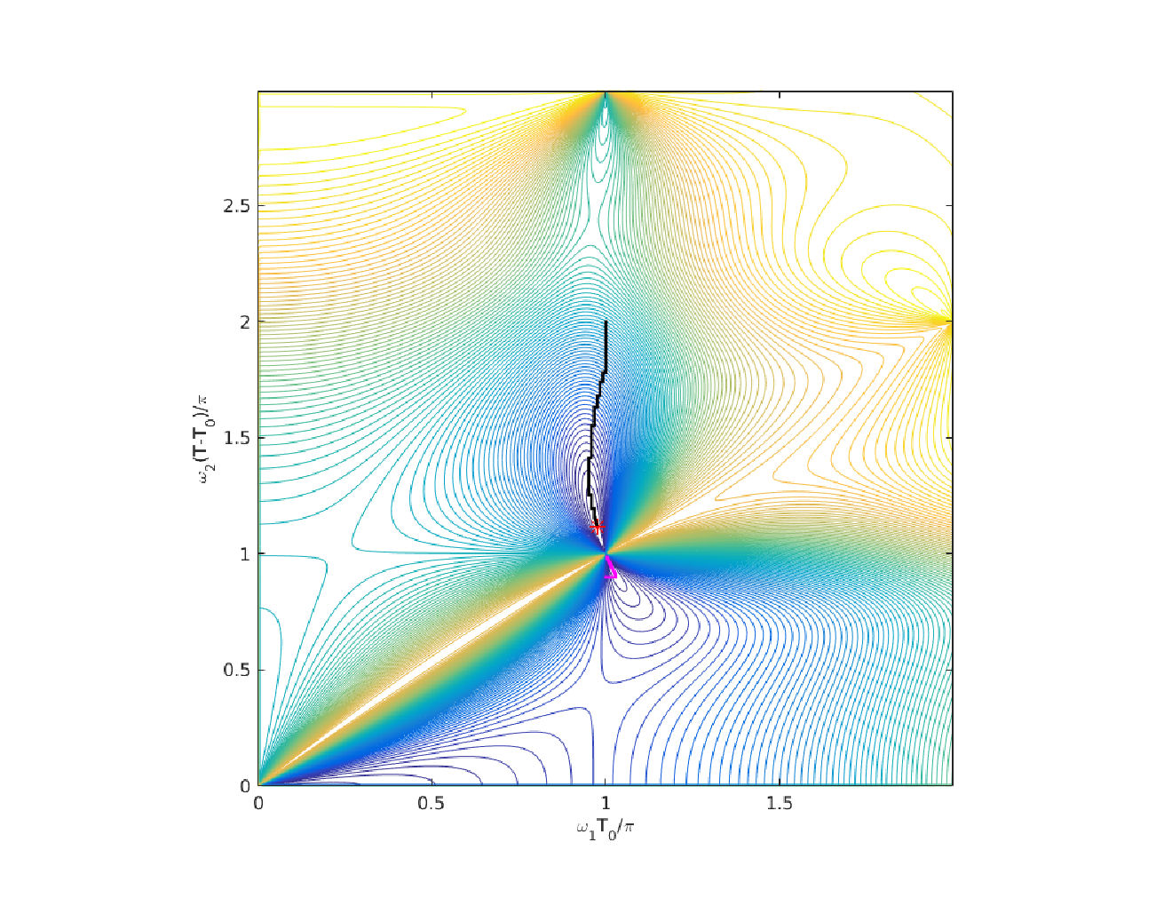
Before moving on, we show the topology of the P⁡(ω1,ω2)P\left(\omega_{1},\omega_{2}\right) function and also its minima locations in ω1\omega_{1} and ω2\omega_{2} space. These will provide useful insights on where to set the initialization point(s) of a possible fast IF algorithm. The data description is provided in the next section. In Figures 2 and 3, we have presented two different dog aortic pressure cycles with the IMF extracted by the means of the brute-force IF Algorithm 1. Figures 2 and 3, top right, show the heat-map plots of P⁡(ω1​T0π,ω2​(T−T0)π)P\left(\frac{\omega_{1}T_{0}}{\pi},\frac{\omega_{2}\left(T-T_{0}\right)}{\pi}\right). The complex nature of P⁡(ω1,ω2)P\left(\omega_{1},\omega_{2}\right) can be seen in these figures. We purposefully plotted PP in the dimensionless coordinates ω1​T0π\frac{\omega_{1}T_{0}}{\pi} and ω2​(T−T0)π\frac{\omega_{2}\left(T-T_{0}\right)}{\pi} to show the behavior of this function with respect to the lattice node locations 𝒩\mathcal{N} defined in (4.20)-(4.22). To have a better view and understanding of the P⁡(ω1,ω2)P\left(\omega_{1},\omega_{2}\right) topology, a contour of P⁡(ω1​T0π,ω2​(T−T0)π)P\left(\frac{\omega_{1}T_{0}}{\pi},\frac{\omega_{2}\left(T-T_{0}\right)}{\pi}\right) is shown in those figures. The general topology of P⁡(ω1​T0π,ω2​(T−T0)π)P\left(\frac{\omega_{1}T_{0}}{\pi},\frac{\omega_{2}\left(T-T_{0}\right)}{\pi}\right), for all aortic or carotid pulse waveforms, is similar to the ones presented in Figures 2 and 3. However, the location of the minimizer is not similar.

Our investigations show that the locations of the minimizers of all PP functions construct two different areas in the dimensionless coordinates ω1​T0π\frac{\omega_{1}T_{0}}{\pi} and ω2​(T−T0)π\frac{\omega_{2}\left(T-T_{0}\right)}{\pi}. We call these areas as the upper lobe and lower lobe. The upper lobe is an area, in 𝒟\mathcal{D}, confined above the line ω2​(T−T0)π=1\frac{\omega_{2}\left(T-T_{0}\right)}{\pi}=1. The lower lobe is an area, in 𝒟\mathcal{D}, confined below the line ω2​(T−T0)π=1\frac{\omega_{2}\left(T-T_{0}\right)}{\pi}=1. This is also the case for human subject data [25]. This type of topology suggests two critical initial guess areas for any non-brute-force algorithm solving (4.1): one set of points in the upper lobe, the other in the lower. In the remaining part of this section, we introduce a fast IF algorithm based on the pattern search method [17].

5.1. Pattern Search IF

The pattern search algorithm (or sometimes called the compass search algorithm) is explained in detail in [17]. For completeness, we have summarized the pattern search algorithm in Algorithm 2. The convergence analysis of this method is expressed in [17].

Initialization.

Let f:ℝn→ℝf:\mathbb{R}^{n}\rightarrow\mathbb{R} be given.

Let x0∈ℝnx_{0}\in\mathbb{R}^{n} be the initial guess.

Let △t​o​l>0\triangle_{tol}>0 be the tolerance used to test for convergence.

Let △0>△t​o​l\triangle_{0}>\triangle_{tol} be the initial value of the step length control parameter.

Algorithm. For each iteration k=1,2,…k=1,2,\ldots

Step 1. Let 𝒟⊕\mathcal{D}_{\oplus} be the set of coordinate directions {±ei|i=1,…,n}\left\{\pm e_{i}\left|i=1,\ldots,n\right.\right\}, where eie_{i} is the ith unit coordinate vector in ℝn\mathbb{R}^{n}.

Step 2. If there exists dk∈𝒟⊕d_{k}\in\mathcal{D}_{\oplus} such that f⁡(xk+△k​dk)<f⁡(xk)f\left(x_{k}+\triangle_{k}d_{k}\right)<f\left(x_{k}\right), then do the following:

  • •

    Set xk+1=xk+△k​dkx_{k+1}=x_{k}+\triangle_{k}d_{k}.

  • •

    Set △k+1=△k\triangle_{k+1}=\triangle_{k}.

Step 3. Otherwise, f⁡(xk+△k​dk)⩾f⁡(xk)f\left(x_{k}+\triangle_{k}d_{k}\right)\geqslant f\left(x_{k}\right) for all dk∈𝒟⊕d_{k}\in\mathcal{D}_{\oplus}, so do the following:

  • •

    Set xk+1=xkx_{k+1}=x_{k}.

  • •

    Set △k+1=12​△k\triangle_{k+1}=\frac{1}{2}\triangle_{k}.

  • •

    If △k+1<△t​o​l\triangle_{k+1}<\triangle_{tol}, then terminate.

Algorithm 2 Pattern Search [17]

The fast IF algorithm, without considering the nodes (4.20), is expressed in Algorithm 3. As mentioned before, what makes Algorithm 3 fast is embedded in three different objects:

  1. (1)

    The initial guess set up in the initialization part of the algorithm.

  2. (2)

    The fast analytic solution at each point iteration defined by (4.17) and (4.16).

  3. (3)

    The pattern search part which is a substitute for the brute force algorithm.

Figure 2, bottom right, shows the results of Algorithm 3. In this figure, when using Algorithm 3, we have used two initial guesses (ω1​T0π=1,ω2​(T−T0)π=2)\left(\frac{\omega_{1}T_{0}}{\pi}=1,\frac{\omega_{2}\left(T-T_{0}\right)}{\pi}=2\right) and (ω1​T0π=1,ω2​(T−T0)π=0.9)\left(\frac{\omega_{1}T_{0}}{\pi}=1,\frac{\omega_{2}\left(T-T_{0}\right)}{\pi}=0.9\right). As depicted on the figure, the initial guess located in the upper lobe has converged towards the true minimizer in 𝒟\mathcal{D}. On a PC having 8 threads, Intel® Core™ i7-4700MQ CPU @ 2.40GHz × 8, running a Matlab implementation of the brute-force Algorithm 1 in parallel takes roughly 8585 seconds. On the other hand, achieving the same minimizer, using a sequential version of the fast Algorithm 3, takes approximately 0.50.5 seconds.

The same test was done for another aortic cycle presented in Figure 3. We used the same initial guesses as before. This time, on the same PC, using the same implementations, the brute-force Algorithm 1 took roughly 8080 seconds and the fast Algorithm 3 took approximately 0.50.5 seconds. These two examples show a speed up of almost 160160 times. In the next section we present more about the statistical accuracy of Algorithm 3 and its physiological capabilities.

Initialization.

Let 𝐟∈ℝn+m\mathbf{f}\in\mathbb{R}^{n+m} be a given discrete aortic/carotid signal with specified T0T_{0} and T−T0T-T_{0}.

Let 𝒟={(ω1,ω2)|0.5⩽ω1​T0π⩽1.5, 0.5⩽ω2​(T−T0)π⩽3}\mathcal{D}=\left\{\left(\omega_{1},\omega_{2}\right)\left|0.5\leqslant\frac{\omega_{1}T_{0}}{\pi}\leqslant 1.5,\,0.5\leqslant\frac{\omega_{2}\left(T-T_{0}\right)}{\pi}\leqslant 3\right.\right\}.

Let G=⋃l=1M{(ω1,ω2)l∈𝒟}G=\bigcup_{l=1}^{M}\left\{\left(\omega_{1},\omega_{2}\right)_{l}\in\mathcal{D}\right\} be the set of MM random initial guesses excluding the nodes (4.20).

Let △​ωt​o​l>0\triangle\omega_{tol}>0 be the convergence tolerance.

Let △​ω0>△​ωt​o​l\triangle\omega_{0}>\triangle\omega_{tol} be the initial step length.

Let ω~k=(ω1k,ω2k)\tilde{\omega}^{k}=\left(\omega_{1}^{k},\omega_{2}^{k}\right) and

P⁡(ω~k)=‖𝐐⁡(ω~k,b1∗​(ω~k),b2∗​(ω~k),𝐭)+p¯∗​(ω~k)​𝟏−𝐟‖22P\left(\tilde{\omega}^{k}\right)=\left\|\mathbf{Q}\left(\tilde{\omega}^{k},b_{1}^{*}\left(\tilde{\omega}^{k}\right),b_{2}^{*}\left(\tilde{\omega}^{k}\right);\mathbf{t}\right)+\bar{p}^{*}\left(\tilde{\omega}^{k}\right)\mathbf{1}-\mathbf{f}\right\|_{2}^{2}

for the kth iteration, defined by (4.17), which is solved using (4.16).

Let 𝒟⊕={±ej|j=1,2}\mathcal{D}_{\oplus}=\left\{\pm e_{j}\left|j=1,2\right.\right\}, where eje_{j} is the jth unit coordinate vector in ℝ2\mathbb{R}^{2}.

Algorithm. For each initial guess ω~i∈G\tilde{\omega}^{i}\in G, i=1,…,Mi=1,\ldots,M, and for each iteration ki=0,1,…k_{i}=0,1,\ldots

Step 1. If there exists 𝐝ki∈𝒟⊕\mathbf{d}_{k_{i}}\in\mathcal{D}_{\oplus} such that P⁡(ω~ki+△​ωki​𝐝ki)<P⁡(ω~ki)P\left(\tilde{\omega}^{k_{i}}+\triangle\omega_{k_{i}}\mathbf{d}_{k_{i}}\right)<P\left(\tilde{\omega}^{k_{i}}\right), then:

  • •

    ω~ki+1=ω~ki+△​ωki​𝐝ki\tilde{\omega}^{k_{i}+1}=\tilde{\omega}^{k_{i}}+\triangle\omega_{k_{i}}\mathbf{d}_{k_{i}}.

  • •

    △​ωki+1=△​ωki\triangle\omega_{k_{i}+1}=\triangle\omega_{k_{i}}.

Step 2. Otherwise, if P⁡(ω~ki+△​ωki​𝐝ki)⩾P⁡(ω~ki)P\left(\tilde{\omega}^{k_{i}}+\triangle\omega_{k_{i}}\mathbf{d}_{k_{i}}\right)\geqslant P\left(\tilde{\omega}^{k_{i}}\right) for all 𝐝ki∈𝒟⊕\mathbf{d}_{k_{i}}\in\mathcal{D}_{\oplus}, then:

  • •

    ω~ki+1=ω~ki\tilde{\omega}^{k_{i}+1}=\tilde{\omega}^{k_{i}}.

  • •

    △​ωki+1=12​△​ωki\triangle\omega_{k_{i}+1}=\frac{1}{2}\triangle\omega_{k_{i}}.

  • •

    If △​ωki+1<△​ωt​o​l\triangle\omega_{k_{i}+1}<\triangle\omega_{tol}, then terminate and ω~i∗=ω~ki+1\tilde{\omega}_{i}^{*}=\tilde{\omega}^{k_{i}+1}.

Step 3. The solution isω~∗=arg⁡mini∈{1,…,M}​P​(ω~i∗)\tilde{\omega}^{*}=\underset{i\in\left\{1,\ldots,M\right\}}{\arg\min}\,P\left(\tilde{\omega}_{i}^{*}\right).

Algorithm 3 Fast IF

6. Real Data Example

The real dog data used in this manuscript is well described in [30]. Since, at the time of the the data retrieval, the data was downloaded with different sampling rates, we re-sampled all six dog data at 500​H​z500\,Hz. We used a modified version of the automatic cycle selection introduced in [36] to pick cycles. Dicrotic notch locations were then found from the picked cycles [19]. We totally extracted 5938459384 acceptable aortic cycles form those six dogs.

6.1. Statistical Accuracy

To check the statistical accuracy of the fast IF algorithm versus the brute-force IF algorithm, we compared the results of these two algorithms on the extracted 5938459384 dog aortic cycles. The brute-force IF algorithm (Algorithm 1) was run over the sample set with a mesh size (minl≠m​(ω1l−ω1m)=minl≠m​(ω2l−ω2m)\underset{l\neq m}{\min}\left(\omega_{1}^{l}-\omega_{1}^{m}\right)=\underset{l\neq m}{\min}\left(\omega_{2}^{l}-\omega_{2}^{m}\right)) of 0.02​π0.02\pi. Algorithm 3 was run on the same sample set of 5938459384 aortic cycles with △​ωt​o​l=0.001\triangle\omega_{tol}=0.001, and △​ω0=0.1\triangle\omega_{0}=0.1, comprising a mesh size of 0.126\frac{0.1}{2^{6}}. The brute-force algorithm has a larger mesh size due to heavy computational cost of this algorithm. The maximum average difference between the IFs found by these two algorithms was found to be less than 0.04750.0475. This difference is smaller than both mesh sizes used for the brute-force and fast IF algorithms. This shows that, on average, the fast IF algorithm (Algorithm 3) reaches the same minima as the brute-force algorithm (Algorithm 1).

6.2. Physiological Observations

To evaluate the new fast IF algorithm (Algorithm 3), we applied the algorithm on the measured aortic pressure signal from one dog experiencing various pharmacological interventions, see Figure 4. During the experiment, the dog was under the following pharmacological influences: infusion of dobutamine (5-20 μ​g/k​g/m​i​n\mu g/kg/min), phenylephrine (2-8 μ​g/k​g/m​i​n\mu g/kg/min) and nitroglycerin (4 μ​g/k​g/m​i​n\mu g/kg/min) during different time intervals.

The third panel, in Figure 4, shows the dosage and duration of each drug in the experiment. In the first phase of the experiment dobutamine has been injected at a low dosage followed by a fluctuation in the dosage of injection. The effect of dobutamine on the cardiovascular system is to increase the strength and force of the heartbeat. Consequently, it forces more blood to circulate throughout the body. In previous works [25, 26], we hypothesized that ω1\omega_{1} would be a representative of heart functionality. We also hypothesized that ω1\omega_{1} and ω2\omega_{2} would try to keep a balance during changes. These hypotheses can be seen during the injection of dobutamine in this figure.

Next, phenylephrine has been injected at a low dosage and the dosage is then increased over time. Phenylephrine is a decongestant which affects the cardiovascular system by shrinking blood vessels. ω2\omega_{2} shows an almost monotone decrease during the infusion of phenylephrine. This is again in qualitative accord with what we presented in [26].

Lastly, nitroglycerin has been injected at a constant dosage. Nitroglycerin helps to dilate the blood vessels. This dilation can be captured with ω2\omega_{2}, as can be seen from the figure. Generally, based on this figure, IFs are able to capture changes in the dynamics of the system under the effects of different drugs.

7. Conclusion

In this paper, we provided a mathematical foundation for the IF model [31]. We showed how to derive an estimation of the IF model (2.1) by considering basic physics principles. More precisely, we showed that the IF model can be estimated from Navier-Stokes and elasticity equations.

We further analysed the IF model (4.1). This helped to introduce a fast algorithm for the IF method (Algorithm 3). What made this algorithm fast was embedded in the proper set up of the initial guesses based on the topology of the problem, fast analytic solution at each point iteration, and substituting the brute force algorithm with a pattern search method. These changes would convert an iterative and brute-force method (Algorithm 1) into an algebraic and iterative method (Algorithm 3). The presented fast algorithm, in this article, has a speed up of more than 100 times compared to the brute-force algorithm provided in [31]. From a statistical perspective, we have also shown that the algorithm presented in this article complies well with the brute-force implementations of this method.

We also showed, on a real dataset, that the fast IF Algorithm 3 can depict correlations between its outputs and infusion of certain drugs. This part of our paper can be subject to further physiological and clinical investigations in a future work.

8. Authors’ Contributions

P.T. conceived of the mathematical and numerical methods of the study, carried out the modeling, programmed the initial code of the method, and drafted the manuscript; H.K. helped with the mathematical and numerical derivations, helped draft and revise the manuscript, and conducted the real data case example; J.K. conducted the brute-force simulations on the real data case example, and helped draft the manuscript. All authors gave final approval for publication.

9. Acknowledgement

We would like to thank Mr. Sean Brady for constructive discussions and editorial comments.

10. Research Ethics

All experiments and procedures were reviewed and approved by the MSU All-University Committee on Animal Use and Care [30].

11. Permission to Carry Out Fieldwork

This study did not have fieldwork.

12. Funding

This work was not funded.

13. Figures

Refer to caption
Figure 1. Simplified cardiovascular system model schematic
Refer to caption
Refer to caption
Refer to caption
Refer to caption
Figure 2. Up-Left: A dog aortic pressure cycle (in blue), its dicrotic notch (black dot), and the IMF (in red). Up-Right: heat-map plot of P⁡(ω1​T0π,ω2​(T−T0)π)P\left(\frac{\omega_{1}T_{0}}{\pi},\frac{\omega_{2}\left(T-T_{0}\right)}{\pi}\right) for the cycle in left with the location of the solution marked with red dot. Down-Left: Contour plot of P⁡(ω1​T0π,ω2​(T−T0)π)P\left(\frac{\omega_{1}T_{0}}{\pi},\frac{\omega_{2}\left(T-T_{0}\right)}{\pi}\right). The location of the minimizer of PP is shown by a red dot. Down-Right: Contour plot of P⁡(ω1​T0π,ω2​(T−T0)π)P\left(\frac{\omega_{1}T_{0}}{\pi},\frac{\omega_{2}\left(T-T_{0}\right)}{\pi}\right) and the location of the minimizer of PP tracked by the pattern search. The true optimum point is marked with a red asterisk. The upper pattern search set (in black) has converged towards the correct optimum. The lower pattern search set (in magenta) has converged to a local minima near the node.
Refer to caption
Refer to caption
Refer to caption
Refer to caption
Figure 3. Up-Left: A dog aortic pressure cycle (in blue), its dicrotic notch (black dot), and the IMF (in red). Up-Right: heat-map plot of P⁡(ω1​T0π,ω2​(T−T0)π)P\left(\frac{\omega_{1}T_{0}}{\pi},\frac{\omega_{2}\left(T-T_{0}\right)}{\pi}\right) for the cycle in left with the location of the solution marked with red dot. Down-Left: Contour plot of P⁡(ω1​T0π,ω2​(T−T0)π)P\left(\frac{\omega_{1}T_{0}}{\pi},\frac{\omega_{2}\left(T-T_{0}\right)}{\pi}\right). The location of the minimizer of PP is shown by a red dot. Down-Right: Contour plot of P⁡(ω1​T0π,ω2​(T−T0)π)P\left(\frac{\omega_{1}T_{0}}{\pi},\frac{\omega_{2}\left(T-T_{0}\right)}{\pi}\right) and the location of the minimizer of PP tracked by the pattern search. The true optimum point is marked with a red asterisk. The lower pattern search set (in black) has converged towards the correct optimum. The upper pattern search set (in magenta) has converged to a local minima near the node.

Refer to caption

Figure 4. Drug effects on ω1\omega_{1} and ω2\omega_{2}. First Panel: The measured aortic pressure waveform recorded in time. Second Panel: Dosage of dobutamine (in red), phenylephrine (in purple), and nitroglycerin (in green) during the aortic pressure measurement. Third Panel: Changes of ω1\omega_{1} in units of bit per minute (bpm) over the measurement time. Each drug effect is projected with its corresponding color. No drug areas are in blue. Fourth Panel: Changes of ω2\omega_{2} in units of bpm over the measurement time. Each drug effect is projected with its corresponding color. No drug areas are in blue.

References

  • [1] Jordi Alastruey, Kim H Parker, and Spencer J Sherwin. Arterial pulse wave haemodynamics. In 11th International Conference on Pressure Surges, pages 401–442. Virtual PiE Led t/a BHR Group: Lisbon, Portugal, 2012.
  • [2] Alberto P Avolio, Mark Butlin, and Andrew Walsh. Arterial blood pressure measurement and pulse wave analysis-their role in enhancing cardiovascular assessment. Physiological measurement, 31(1):R1, 2009.
  • [3] DAVID S Berger, JK Li, and ABRAHAM Noordergraaf. Differential effects of wave reflections and peripheral resistance on aortic blood pressure: a model-based study. American Journal of Physiology-Heart and Circulatory Physiology, 266(4):H1626–H1642, 1994.
  • [4] D.P. Bertsekas. Nonlinear programming. Athena Scientific, 1999.
  • [5] OF Borisenko and LI Minchenko. Directional derivatives of the maximum function. Cybernetics and Systems Analysis, 28(2):309–312, 1992.
  • [6] Barry A Borlaug, Carolyn SP Lam, Véronique L Roger, Richard J Rodeheffer, and Margaret M Redfield. Contractility and ventricular systolic stiffening in hypertensive heart disease: insights into the pathogenesis of heart failure with preserved ejection fraction. Journal of the American College of Cardiology, 54(5):410–418, 2009.
  • [7] S. Boyd and L. Vandenberghe. Convex optimization. Cambridge university press, 2004.
  • [8] Mirko De Melis, Umberto Morbiducci, Ernst R Rietzschel, Marc De Buyzere, Ahmad Qasem, Luc Van Bortel, Tom Claessens, Franco M Montevecchi, Albert Avolio, and Patrick Segers. Blood pressure waveform analysis by means of wavelet transform. Medical & biological engineering & computing, 47(2):165–173, 2009.
  • [9] S.J. Denardo, R. Nandyala, G.L. Freeman, G.L. Pierce, and W.W. Nichols. Pulse wave analysis of the aortic pressure waveform in severe left ventricular systolic dysfunctionclinical perspective. Circulation: Heart Failure, 3(1):149–156, 2010.
  • [10] Marc Dewey, Mira Müller, Stephan Eddicks, Dirk Schnapauff, Florian Teige, Wolfgang Rutsch, Adrian C Borges, and Bernd Hamm. Evaluation of global and regional left ventricular function with 16-slice computed tomography, biplane cineventriculography, and two-dimensional transthoracic echocardiography: comparison with magnetic resonance imaging. Journal of the American College of Cardiology, 48(10):2034–2044, 2006.
  • [11] Nick Gould and Philippe L Toint. Preprocessing for quadratic programming. Mathematical Programming, 100(1):95–132, 2004.
  • [12] Johannes Greupner, Elke Zimmermann, Andrea Grohmann, Hans-Peter Dübel, Till Althoff, Adrian C Borges, Wolfgang Rutsch, Peter Schlattmann, Bernd Hamm, and Marc Dewey. Head-to-head comparison of left ventricular function assessment with 64-row computed tomography, biplane left cineventriculography, and both 2-and 3-dimensional transthoracic echocardiography: comparison with magnetic resonance imaging as the reference standard. Journal of the American College of Cardiology, 59(21):1897–1907, 2012.
  • [13] W Dallas Hall. Stephen hales: theologian, botanist, physiologist, discoverer of hemodynamics. Clinical cardiology, 10(8):487–489, 1987.
  • [14] Rainer Hoffmann, Giuseppe Barletta, Stephan von Bardeleben, Jean Louis Vanoverschelde, Jaroslaw Kasprzak, Christian Greis, and Harald Becher. Analysis of left ventricular volumes and function: a multicenter comparison of cardiac magnetic resonance imaging, cine ventriculography, and unenhanced and contrast-enhanced two-dimensional and three-dimensional echocardiography. Journal of the American Society of Echocardiography, 27(3):292–301, 2014.
  • [15] Rainer Hoffmann, Stephan von Bardeleben, Folkert ten Cate, Adrian C Borges, Jaroslaw Kasprzak, Christian Firschke, Stephane Lafitte, Nidal Al-Saadi, Stefanie Kuntz-Hehner, Marc Engelhardt, et al. Assessment of systolic left ventricular function: a multi-centre comparison of cineventriculography, cardiac magnetic resonance imaging, unenhanced and contrast-enhanced echocardiography. European Heart Journal, 26(6):607–616, 2005.
  • [16] Robert Hooke and Terry A Jeeves. “direct search”solution of numerical and statistical problems. Journal of the ACM (JACM), 8(2):212–229, 1961.
  • [17] T.G. Kolda, R.M. Lewis, and V. Torczon. Optimization by direct search: New perspectives on some classical and modern methods. SIAM review, 45(3):385–482, 2003.
  • [18] Stephane Laurent, John Cockcroft, Luc Van Bortel, Pierre Boutouyrie, Cristina Giannattasio, Daniel Hayoz, Bruno Pannier, Charalambos Vlachopoulos, Ian Wilkinson, and Harry Struijker-Boudier. Expert consensus document on arterial stiffness: methodological issues and clinical applications. European heart journal, 27(21):2588–2605, 2006.
  • [19] Bing Nan Li, Ming Chui Dong, and Mang I Vai. On an automatic delineator for arterial blood pressure waveforms. Biomedical Signal Processing and Control, 5(1):76–81, 2010.
  • [20] D. Lloyd-Jones, R.J. Adams, T.M. Brown, M. Carnethon, S. Dai, G. De Simone, T.B. Ferguson, E. Ford, K. Furie, C. Gillespie, et al. Heart disease and stroke statistics 2010 update. Circulation, 121(7):e46–e215, 2010.
  • [21] W.R. Milnor. Hemodynamics. Williams & Wilkins, 1989.
  • [22] Dariush Mozaffarian, Emelia J Benjamin, Alan S Go, Donna K Arnett, Michael J Blaha, Mary Cushman, Sandeep R Das, Sarah de Ferranti, Jean-pierre Després, Heather J Fullerton, et al. Executive summary: Heart disease and stroke statistics-2016 update: A report from the american heart association. Circulation, 133(4):447, 2016.
  • [23] W.W. Nichols and M.F. O’Rourke. McDonald’s blood flow in arteries: theoretical, experimental, and clinical principles. CRC Press, 2011.
  • [24] W.W. Nichols, M.F. O’Rourke, C. Hartley, et al. McDonald’s blood flow in arteries: theoretical, experimental and clinical principles, volume 340809418. Hodder Arnold London, 2005.
  • [25] Niema M Pahlevan, Derek G Rinderknecht, Peyman Tavallali, Marianne Razavi, Thao T Tran, Michael W Fong, Robert A Kloner, Marie Csete, and Morteza Gharib. Noninvasive iphone measurement of left ventricular ejection fraction using intrinsic frequency methodology. Critical care medicine, 2017.
  • [26] Niema M Pahlevan, Peyman Tavallali, Derek G Rinderknecht, Danny Petrasek, Ray V Matthews, Thomas Y Hou, and Morteza Gharib. Intrinsic frequency for a systems approach to haemodynamic waveform analysis with clinical applications. Journal of The Royal Society Interface, 11(98):20140617, 2014.
  • [27] Kim H Parker. A brief history of arterial wave mechanics. Medical and Biological Engineering and Computing, 47(2):111–118, 2009.
  • [28] BN Pshenichnyi. Necessary conditions for an extremum. New York, 1971.
  • [29] Marek W Rajzer, Wiktoria Wojciechowska, Marek Klocek, Ilona Palka, Malgorzata Brzozowska-Kiszka, and Kalina Kawecka-Jaszcz. Comparison of aortic pulse wave velocity measured by three techniques: Complior, sphygmocor and arteriograph. Journal of hypertension, 26(10):2001–2007, 2008.
  • [30] Gokul Swamy, Jacob Kuiper, Madhu SR Gudur, N Bari Olivier, and Ramakrishna Mukkamala. Continuous left ventricular ejection fraction monitoring by aortic pressure waveform analysis. Annals of biomedical engineering, 37(6):1055, 2009.
  • [31] Peyman Tavallali, Thomas Y Hou, Derek G Rinderknecht, and Niema M Pahlevan. On the convergence and accuracy of the cardiovascular intrinsic frequency method. Royal Society Open Science, 2(12):150475, 2015.
  • [32] Lloyd N Trefethen and David Bau III. Numerical linear algebra, volume 50. Siam, 1997.
  • [33] Yuh-Ying Lin Wang, Wah-Keung Sze, Jian-Guo Bau, Sheng-Hung Wang, Ming-Yie Jan, Tse-Lin Hsu, and Wei-Kung Wang. The ventricular-arterial coupling system can be analyzed by the eigenwave modes of the whole arterial system. Applied Physics Letters, 92(15):153901, 2008.
  • [34] Nicolaas Westerhof, Frederik Bosman, Cornelis J De Vries, and Abraham Noordergraaf. Analog studies of the human systemic arterial tree. Journal of biomechanics, 2(2):121–143, 1969.
  • [35] Mair Zamir and M Zamir. The physics of pulsatile flow. Springer, 2000.
  • [36] W Zong, T Heldt, GB Moody, and RG Mark. An open-source algorithm to detect onset of arterial blood pressure pulses. In Computers in Cardiology, 2003, pages 259–262. IEEE, 2003.

Appendix A

In this appendix, we show how one can derive (3.2) and (3.1), from the Navier-Stokes and elasticity equations. Having xx, rr and θ\theta as the cylindrical coordinate system, with xx in the direction of the aortic length, the momentum and the continuity equations are

(13.1) ρ⁡(∂u∂t+u​∂u∂x+v​∂u∂r+ωr​∂u∂θ)+∂P∂x=μ⁡(∂2u∂x2+∂2u∂r2+1r​∂u∂r+1r2​∂2u∂θ2),\begin{array}[]{c}\rho\left(\frac{\partial u}{\partial t}+u\frac{\partial u}{\partial x}+v\frac{\partial u}{\partial r}+\frac{\omega}{r}\frac{\partial u}{\partial\theta}\right)+\frac{\partial P}{\partial x}=\\ \mu\left(\frac{\partial^{2}u}{\partial x^{2}}+\frac{\partial^{2}u}{\partial r^{2}}+\frac{1}{r}\frac{\partial u}{\partial r}+\frac{1}{r^{2}}\frac{\partial^{2}u}{\partial\theta^{2}}\right),\end{array}
(13.2) ρ⁡(∂v∂t+u​∂v∂x+v​∂v∂r+wr​∂v∂θ−w2r)+∂P∂r=μ⁡(∂2v∂x2+∂2v∂r2+1r​∂v∂r−vr2+1r2​∂2v∂θ2−2r2​∂w∂θ),\begin{array}[]{c}\rho\left(\frac{\partial v}{\partial t}+u\frac{\partial v}{\partial x}+v\frac{\partial v}{\partial r}+\frac{w}{r}\frac{\partial v}{\partial\theta}-\frac{w^{2}}{r}\right)+\frac{\partial P}{\partial r}=\\ \mu\left(\frac{\partial^{2}v}{\partial x^{2}}+\frac{\partial^{2}v}{\partial r^{2}}+\frac{1}{r}\frac{\partial v}{\partial r}-\frac{v}{r^{2}}+\frac{1}{r^{2}}\frac{\partial^{2}v}{\partial\theta^{2}}-\frac{2}{r^{2}}\frac{\partial w}{\partial\theta}\right),\end{array}
(13.3) ρ⁡(∂w∂t+u​∂w∂x+v​∂w∂r+wr​∂w∂θ+v​wr)+1r​∂P∂θ=μ⁡(∂2w∂x2+∂2w∂r2+1r​∂w∂r−wr2+1r2​∂2w∂θ2+2r2​∂v∂θ),\begin{array}[]{c}\rho\left(\frac{\partial w}{\partial t}+u\frac{\partial w}{\partial x}+v\frac{\partial w}{\partial r}+\frac{w}{r}\frac{\partial w}{\partial\theta}+\frac{vw}{r}\right)+\frac{1}{r}\frac{\partial P}{\partial\theta}=\\ \mu\left(\frac{\partial^{2}w}{\partial x^{2}}+\frac{\partial^{2}w}{\partial r^{2}}+\frac{1}{r}\frac{\partial w}{\partial r}-\frac{w}{r^{2}}+\frac{1}{r^{2}}\frac{\partial^{2}w}{\partial\theta^{2}}+\frac{2}{r^{2}}\frac{\partial v}{\partial\theta}\right),\end{array}
(13.4) ∂u∂x+∂v∂r+vr+1r​∂w∂θ=0.\frac{\partial u}{\partial x}+\frac{\partial v}{\partial r}+\frac{v}{r}+\frac{1}{r}\frac{\partial w}{\partial\theta}=0.

Here, uu, vv and ww are velocity vector components in xx, rr and θ\theta directions, respectively. We assume that aorta is a straight and sufficiently long tube with constant circular cross section with the tube wall following classical elasticity theory dynamics and blood is considered to be an incompressible Newtonian fluid with the velocity field being axisymmetric. In the absents of any external forces causing flow rotation, the assumption that the flow field is symmetrical about the longitudinal axis of the tube is justified. This means w=∂w∂θ=∂v∂θ=∂u∂θ=∂P∂θ=0w=\frac{\partial w}{\partial\theta}=\frac{\partial v}{\partial\theta}=\frac{\partial u}{\partial\theta}=\frac{\partial P}{\partial\theta}=0. Hence, Equations (13.1)-(13.4) will be simplified as

(13.5) ρ⁡(∂u∂t+u​∂u∂x+v​∂u∂r)+∂P∂x=μ⁡(∂2u∂x2+∂2u∂r2+1r​∂u∂r),\rho\left(\frac{\partial u}{\partial t}+u\frac{\partial u}{\partial x}+v\frac{\partial u}{\partial r}\right)+\frac{\partial P}{\partial x}=\mu\left(\frac{\partial^{2}u}{\partial x^{2}}+\frac{\partial^{2}u}{\partial r^{2}}+\frac{1}{r}\frac{\partial u}{\partial r}\right),
(13.6) ρ⁡(∂v∂t+u​∂v∂x+v​∂v∂r)+∂P∂r=μ⁡(∂2v∂x2+∂2v∂r2+1r​∂v∂r−vr2),\rho\left(\frac{\partial v}{\partial t}+u\frac{\partial v}{\partial x}+v\frac{\partial v}{\partial r}\right)+\frac{\partial P}{\partial r}=\mu\left(\frac{\partial^{2}v}{\partial x^{2}}+\frac{\partial^{2}v}{\partial r^{2}}+\frac{1}{r}\frac{\partial v}{\partial r}-\frac{v}{r^{2}}\right),
(13.7) ∂u∂x+∂v∂r+vr=0.\frac{\partial u}{\partial x}+\frac{\partial v}{\partial r}+\frac{v}{r}=0.

Since the radius of the tube aa is smaller than the length of the tube, a≪ha\ll h, and also the average velocity of the blood in aorta is smaller than the speed of wave propagation [35], we have

(13.8) u​∂u∂x≪∂u∂t,u\frac{\partial u}{\partial x}\ll\frac{\partial u}{\partial t},
(13.9) v​∂u∂r≪∂u∂t,v\frac{\partial u}{\partial r}\ll\frac{\partial u}{\partial t},
(13.10) u​∂v∂x≪∂v∂t,u\frac{\partial v}{\partial x}\ll\frac{\partial v}{\partial t},
(13.11) v​∂v∂r≪∂v∂t,v\frac{\partial v}{\partial r}\ll\frac{\partial v}{\partial t},
(13.12) ∂2u∂x2≪∂2u∂r2,\frac{\partial^{2}u}{\partial x^{2}}\ll\frac{\partial^{2}u}{\partial r^{2}},
(13.13) ∂2v∂x2≪∂2v∂r2.\frac{\partial^{2}v}{\partial x^{2}}\ll\frac{\partial^{2}v}{\partial r^{2}}.

Using these, Equations (13.5)-(13.7) will reduce to

(13.14) ρ​∂u∂t+∂P∂x=μ⁡(∂2u∂r2+1r​∂u∂r)\rho\frac{\partial u}{\partial t}+\frac{\partial P}{\partial x}=\mu\left(\frac{\partial^{2}u}{\partial r^{2}}+\frac{1}{r}\frac{\partial u}{\partial r}\right)
(13.15) ρ​∂v∂t+∂P∂r=μ⁡(∂2v∂r2+1r​∂v∂r−vr2)\rho\frac{\partial v}{\partial t}+\frac{\partial P}{\partial r}=\mu\left(\frac{\partial^{2}v}{\partial r^{2}}+\frac{1}{r}\frac{\partial v}{\partial r}-\frac{v}{r^{2}}\right)
(13.16) ∂u∂x+∂v∂r+vr=0\frac{\partial u}{\partial x}+\frac{\partial v}{\partial r}+\frac{v}{r}=0

It is important to mention that the velocity vector is a function of time and location. In other words, we have u⁡(x,r,t)u\left(x,r,t\right) and v⁡(x,r,t)v\left(x,r,t\right). Based on the characteristic length of the problem, pressure PP can be assumed to be a function of xx and tt and not rr, i.e. P⁡(x,t)P\left(x,t\right) (See Chapter 5 of [35]). Hence we can set ∂P∂r≈0\frac{\partial P}{\partial r}\approx 0 in (13.15).

Momentum Equations:

Considering (13.14), one can integrate both sides with respect to the differential element of the area 2​π​r​d​r2\pi rdr.

(13.17) ∫0a⁡(x,t)2​π​r​ρ​∂u∂t​𝑑r+∫0a⁡(x,t)2​π​r​∂P∂x​𝑑r=∫0a⁡(x,t)2​π​r​μ​(∂2u∂r2+1r​∂u∂r)​𝑑r.\intop_{0}^{a\left(x,t\right)}2\pi r\rho\frac{\partial u}{\partial t}dr+\intop_{0}^{a\left(x,t\right)}2\pi r\frac{\partial P}{\partial x}dr=\intop_{0}^{a\left(x,t\right)}2\pi r\mu\left(\frac{\partial^{2}u}{\partial r^{2}}+\frac{1}{r}\frac{\partial u}{\partial r}\right)dr.

The upper boundary of this integral is the radius a⁡(x,t)a\left(x,t\right) of the tube. We know that the flow Q⁡(x,t)Q\left(x,t\right) is defined as

(13.18) Q⁡(x,t)=∫0a⁡(x,t)2​π​r​u​(x,r,t)​𝑑r.Q\left(x,t\right)=\intop_{0}^{a\left(x,t\right)}2\pi ru\left(x,r,t\right)dr.

Hence, using Leibniz rule we can find the derivative of the flow with respect to time as

(13.19) ∂Q∂t​(x,t)=∫0a⁡(x,t)2​π​r​∂u∂t​(x,r,t)​𝑑r+2​π​a​(x,t)​∂a∂t​(x,t)​u​(x,a⁡(x,t),t).\frac{\partial Q}{\partial t}\left(x,t\right)=\intop_{0}^{a\left(x,t\right)}2\pi r\frac{\partial u}{\partial t}\left(x,r,t\right)dr+2\pi a\left(x,t\right)\frac{\partial a}{\partial t}\left(x,t\right)u\left(x,a\left(x,t\right),t\right).

Considering no slip boundary condition u⁡(x,a⁡(x,t),t)=0u\left(x,a\left(x,t\right),t\right)=0 on the tube wall, Equation (13.19) reduces to

(13.20) ∂Q∂t​(x,t)=∫0a⁡(x,t)2​π​r​∂u∂t​(x,r,t)​𝑑r.\frac{\partial Q}{\partial t}\left(x,t\right)=\intop_{0}^{a\left(x,t\right)}2\pi r\frac{\partial u}{\partial t}\left(x,r,t\right)dr.

Therefore Equation (13.17) will be simplified to

(13.21) ρ​∂Q∂t+π​a2​∂P∂x=2​π​μ​∫0a⁡(x,t)r⁡(∂2u∂r2+1r​∂u∂r)​𝑑r.\rho\frac{\partial Q}{\partial t}+\pi a^{2}\frac{\partial P}{\partial x}=2\pi\mu\intop_{0}^{a\left(x,t\right)}r\left(\frac{\partial^{2}u}{\partial r^{2}}+\frac{1}{r}\frac{\partial u}{\partial r}\right)dr.

Since we have

(13.22) ∫0a⁡(x,t)r⁡(∂2u∂r2+1r​∂u∂r)​𝑑r=∫0a⁡(x,t)∂(r​∂u∂r)∂r​𝑑r,\intop_{0}^{a\left(x,t\right)}r\left(\frac{\partial^{2}u}{\partial r^{2}}+\frac{1}{r}\frac{\partial u}{\partial r}\right)dr=\intop_{0}^{a\left(x,t\right)}\frac{\partial\left(r\frac{\partial u}{\partial r}\right)}{\partial r}dr,

Equation (13.21) would become

(13.23) ρ​∂Q∂t+π​a2​∂P∂x=2​π​μ​r​∂u∂r∣0a⁡(x,t).\rho\frac{\partial Q}{\partial t}+\pi a^{2}\frac{\partial P}{\partial x}=2\pi\mu r\frac{\partial u}{\partial r}\mid_{0}^{a\left(x,t\right)}.

Using separation of variables u⁡(x,r,t)=U⁡(r)​u¯​(x,t)u\left(x,r,t\right)=U\left(r\right)\bar{u}\left(x,t\right), for some function U⁡(r)U\left(r\right) and u¯​(x,t)\bar{u}\left(x,t\right), Equation (13.23) will be simplified to

(13.24) ρ​∂Q∂t+π​a2​∂P∂x=2​π​μ​a​(x,t)​u¯​(x,t)​(d​Ud​r∣a⁡(x,t)).\rho\frac{\partial Q}{\partial t}+\pi a^{2}\frac{\partial P}{\partial x}=2\pi\mu a\left(x,t\right)\bar{u}\left(x,t\right)\left(\frac{dU}{dr}\mid_{a\left(x,t\right)}\right).

From Equation (13.18) and u⁡(x,r,t)=U⁡(r)​u¯​(x,t)u\left(x,r,t\right)=U\left(r\right)\bar{u}\left(x,t\right), we have

(13.25) u¯​(x,t)=Q⁡(x,t)​(2​π​∫0a⁡(x,t)r​U​(r)​𝑑r)−1.\bar{u}\left(x,t\right)=Q\left(x,t\right)\left(2\pi\intop_{0}^{a\left(x,t\right)}rU\left(r\right)dr\right)^{-1}.

Therefore equation (13.24) will be simplified to

(13.26) ρ​∂Q∂t​(x,t)+π​a2​(x,t)​∂P∂x​(x,t)=μ​a​(x,t)​(d​Ud​r∣a⁡(x,t))​(∫0a⁡(x,t)r​U​(r)​𝑑r)−1​Q​(x,t).\rho\frac{\partial Q}{\partial t}\left(x,t\right)+\pi a^{2}\left(x,t\right)\frac{\partial P}{\partial x}\left(x,t\right)=\mu a\left(x,t\right)\left(\frac{dU}{dr}\mid_{a\left(x,t\right)}\right)\left(\intop_{0}^{a\left(x,t\right)}rU\left(r\right)dr\right)^{-1}Q\left(x,t\right).

From (13.26), we can relabel some terms and introduce the inductance ℒ\mathcal{L} and resistance ℛ\mathcal{R} as

(13.27) ℒ⁡(x,t)=ρπ​a2​(x,t),\mathcal{L}\left(x,t\right)=\frac{\rho}{\pi a^{2}\left(x,t\right)},
(13.28) ℛ⁡(x,t)=−μ⁡(d​Ud​r∣a⁡(x,t))​(π​a​(x,t)​∫0a⁡(x,t)r​U​(r)​𝑑r)−1.\mathcal{R}\left(x,t\right)=-\mu\left(\frac{dU}{dr}\mid_{a\left(x,t\right)}\right)\left(\pi a\left(x,t\right)\intop_{0}^{a\left(x,t\right)}rU\left(r\right)dr\right)^{-1}.

These will convert (13.26) into

(13.29) −∂P∂x​(x,t)=ℒ⁡(x,t)​∂Q∂t​(x,t)+ℛ⁡(x,t)​Q​(x,t).-\frac{\partial P}{\partial x}\left(x,t\right)=\mathcal{L}\left(x,t\right)\frac{\partial Q}{\partial t}\left(x,t\right)+\mathcal{R}\left(x,t\right)Q\left(x,t\right).

Continuity Equation:

Again, applying Leibniz rule to equation (13.18) we can find the derivative of the flow with respect to xx

(13.30) ∂Q∂x​(x,t)=∫0a⁡(x,t)2​π​r​∂u∂x​(x,r,t)​𝑑r+2​π​a​(x,t)​∂a∂x​(x,t)​u​(x,a⁡(x,t),t).\frac{\partial Q}{\partial x}\left(x,t\right)=\intop_{0}^{a\left(x,t\right)}2\pi r\frac{\partial u}{\partial x}\left(x,r,t\right)dr+2\pi a\left(x,t\right)\frac{\partial a}{\partial x}\left(x,t\right)u\left(x,a\left(x,t\right),t\right).

Considering the no slip boundary condition u⁡(x,a⁡(x,t),t)=0u\left(x,a(x,t),t\right)=0, equation (13.30) reduces to

(13.31) ∂Q∂x​(x,t)=∫0a⁡(x,t)2​π​r​∂u∂x​(x,r,t)​𝑑r.\frac{\partial Q}{\partial x}\left(x,t\right)=\intop_{0}^{a\left(x,t\right)}2\pi r\frac{\partial u}{\partial x}\left(x,r,t\right)dr.

Now, we can rewrite the equation of continuity (13.16) as

(13.32) ∫0a⁡(x,t)2​π​r​∂u∂x​𝑑r+∫0a⁡(x,t)2​π​(r​∂v∂r+v)​𝑑r=0.\intop_{0}^{a\left(x,t\right)}2\pi r\frac{\partial u}{\partial x}dr+\intop_{0}^{a\left(x,t\right)}2\pi\left(r\frac{\partial v}{\partial r}+v\right)dr=0.

This equation, using (13.31), will result in

(13.33) ∂Q∂x+∫0a⁡(x,t)2​π​∂(r​v)∂r​𝑑r=0.\frac{\partial Q}{\partial x}+\intop_{0}^{a\left(x,t\right)}2\pi\frac{\partial\left(rv\right)}{\partial r}dr=0.

Simplifying the latter would show that

(13.34) ∂Q∂x+2​π​a​(x,t)​v​(a⁡(x,t))=0.\frac{\partial Q}{\partial x}+2\pi a\left(x,t\right)v\left(a\left(x,t\right)\right)=0.

We note that v⁡(a⁡(x,t))=∂a∂t​(x,t)v\left(a\left(x,t\right)\right)=\frac{\partial a}{\partial t}\left(x,t\right). Hence, having A=π​a2​(x,t)A=\pi a^{2}\left(x,t\right), we can conclude ∂A∂t=2​π​a​(x,t)​v​(a⁡(x,t))\frac{\partial A}{\partial t}=2\pi a\left(x,t\right)v\left(a\left(x,t\right)\right). Consequently, Equation (13.34) can be written as

(13.35) ∂Q∂x+∂A∂t=0.\frac{\partial Q}{\partial x}+\frac{\partial A}{\partial t}=0.

Using the chain rule we have

(13.36) ∂A∂t=∂A∂P​∂P∂t.\frac{\partial A}{\partial t}=\frac{\partial A}{\partial P}\frac{\partial P}{\partial t}.

Considering the wave speed c0c_{0} of an incompressible fluid in an elastic tube we have ∂A∂P=Aρ​c02\frac{\partial A}{\partial P}=\frac{A}{\rho c_{0}^{2}} [27]. Matching this with Equations (13.35) and (13.33) would result in

(13.37) ∂Q∂x​(x,t)+π​a2​(x,t)ρ​c02​∂P∂t​(x,t)=0.\frac{\partial Q}{\partial x}\left(x,t\right)+\frac{\pi a^{2}\left(x,t\right)}{\rho c_{0}^{2}}\frac{\partial P}{\partial t}\left(x,t\right)=0.

In this equation, we can relabel π​a2​(x,t)ρ​c02\frac{\pi a^{2}\left(x,t\right)}{\rho c_{0}^{2}} as the compliance 𝒞⁡(x,t)\mathcal{C}\left(x,t\right). Hence, (13.37) would become

(13.38) −∂Q∂x​(x,t)=𝒞⁡(x,t)​∂P∂t​(x,t).-\frac{\partial Q}{\partial x}\left(x,t\right)=\mathcal{C}\left(x,t\right)\frac{\partial P}{\partial t}\left(x,t\right).

Wave Equations:

As depicted so far, using the approximations in this appendix, and considering the mentioned assumptions, we can characterize the wave dynamics of the blood flow in aorta using the hyperbolic equations (13.38) and (13.29), namely

(13.39) −∂Q∂x​(x,t)=𝒞⁡(x,t)​∂P∂t​(x,t),-\frac{\partial Q}{\partial x}\left(x,t\right)=\mathcal{C}\left(x,t\right)\frac{\partial P}{\partial t}\left(x,t\right),
(13.40) −∂P∂x​(x,t)=ℒ⁡(x,t)​∂Q∂t​(x,t)+ℛ⁡(x,t)​Q​(x,t).-\frac{\partial P}{\partial x}\left(x,t\right)=\mathcal{L}\left(x,t\right)\frac{\partial Q}{\partial t}\left(x,t\right)+\mathcal{R}\left(x,t\right)Q\left(x,t\right).

The coefficients 𝒞⁡(x,t)\mathcal{C}\left(x,t\right), ℒ⁡(x,t)\mathcal{L}\left(x,t\right) and ℛ⁡(x,t)\mathcal{R}\left(x,t\right), in Equations (13.38) and (13.29), are all positive and functions of a⁡(x,t)a\left(x,t\right). However, since a⁡(x,t)a\left(x,t\right) is not changing drastically with respect to xx and tt, we can approximate all these coefficients with their corresponding constant mean values CC, LL and RR. Using this approximation, we can rewrite the wave equations as

(13.41) −∂Q∂x​(x,t)=C​∂P∂t​(x,t),-\frac{\partial Q}{\partial x}\left(x,t\right)=C\frac{\partial P}{\partial t}\left(x,t\right),
(13.42) −∂P∂x​(x,t)=L​∂Q∂t​(x,t)+R​Q​(x,t).-\frac{\partial P}{\partial x}\left(x,t\right)=L\frac{\partial Q}{\partial t}\left(x,t\right)+RQ\left(x,t\right).