Impact of different time series aggregation methods on optimal energy system design
Abstract
Modelling renewable energy systems is a computationally-demanding task due to the high fluctuation of supply and demand time series. To reduce the scale of these, this paper discusses different methods for their aggregation into typical periods. Each aggregation method is applied to a different type of energy system model, making the methods fairly incomparable.
To overcome this, the different aggregation methods are first extended so that they can be applied to all types of multidimensional time series and then compared by applying them to different energy system configurations and analyzing their impact on the cost optimal design.
It was found that regardless of the method, time series aggregation allows for significantly reduced computational resources. Nevertheless, averaged values lead to underestimation of the real system cost in comparison to the use of representative periods from the original time series. The aggregation method itself – e.g., k-means clustering – plays a minor role. More significant is the system considered: Energy systems utilizing centralized resources require fewer typical periods for a feasible system design in comparison to systems with a higher share of renewable feed-in. Furthermore, for energy systems based on seasonal storage, currently existing models’ integration of typical periods is not suitable.
Keywords:
Energy systems , Renewable energies , Mixed integer linear programming , Typical periods , Cluster analysis , Extreme periods , Time-series aggregationNomenclature
- Variables
-
Binary variable determining the existance of a technology
-
Representative values of a typical period
-
Scaling of a device
-
Energy flow between two components
-
State of charge
- y
Binary variable determining if the candidate is a cluster center
- z
Binary variable determining candidate cluster assignment
- Parameters
-
Duration of a single time step
-
Efficiency
-
Lifetime
- C
Set of periods inside a cluster
- L
Set of component connections
- N
Size of an index set
- x
Normalized candidate value
- Subscripts and sets
-
Energy type
-
Index of the Transformer class
-
Index of the Collector class
-
Index of the Source/Sink class
-
Index of the Storage class
- a
Attribute represented by a time series
- d
Considered device or technology
- g
Time step index inside a period
- i
Candidate period index
- k
Typical period index
- t
Time step index of the full series
- Abbreviations
-
Capital Recovery Factor
-
Lower bound
-
Upper bound
- CAPEX
Specific capital expenditure
- CHP
Combined Heat and Power plant
- GHI
Global Horizontal Irradiance
- OPEX
Specific fix operational expenditure
- RMSE
Root Mean Squared Error
- WACC
Weighted Average Cost of Capital
1 Introduction
Developing an energy system design that minimizes costs and environmental impact is a complex task due to the spatial and temporal gap between energy production and demand. In consequence, optimization algorithms are required for solving these design problems [1, 2, 3, 4, 5, 6, 7, 8, 9, 10, 11].
However, the algorithms used hitherto are computationally demanding: The size of the input data directly influences that of the related optimization problem, and with it the requirement for processing resources. For this reason, it is often necessary to simplify the design problem in advance.
Therefore, different options for complexity reduction exist and include: Spatial aggregation which reduces the number of nodes in an energy system network [12]; simplifying the technology models by reducing nonlinearities or discontinuities so as to avoid non-convexity of the program [13, 14]; and temporal aggregation, which creates typical periods representing the original input time series.
The creation of recurring periods is popular because of the existing patterns in the hourly, daily and seasonal variation for the majority of design relevant time series. Therefore, it is reasonable to reduce redundant data until the minimal representative data set required for the problem is reached. Figure 1 visualizes this redundancy by showing the result of a Fast Fourier Transformation (FFT) of different time series that are typically required for an energy system design. The frequencies with the highest amplitudes are highlighted and are, as anticipated, the daily and annual variations.
0

For this reason, many different methods for the selection of typical periods have been presented. Aside from custom exact optimization methods [17, 18], and graphical methods [19], the majority use heuristic methods or greedy clustering algorithms for the aggregation of typical periods. Creating representative days by averaging time series, for example over a type of day defined by month or weekday, has been popular [20, 21, 22, 23]. [24] refers to it as time-chronological averaging. Recent attempts use the k-means clustering [25, 26, 27, 28], hierarchical clustering [29, 30], or k-medoids clustering - either based on a greedy algorithm [31, 32] or an exact solution of a MILP [33, 34] - for the selection of typical periods. Nevertheless, each method is applied to a different system and it is difficult to identify which is the most suitable. While Schuetz et al. [35] compare methods for building energy systems, they note that future research should focus on the appropriateness of clustering algorithms for different design applications. Moreover, the period length should be varied so as to assess the impact of storage effects.
A further difficulty is that the system considered determines the minimal required dataset. For renewable energy systems, a higher resolution of the input times-series is required than with their fossil counterparts [36]. For conventional system design, it could be sufficient to reduce the dataset to a few time steps [27], while for a storage based system design different typical weeks are required [37, 30].
In summary, the following open research questions present themselves:
- 1.
Which time-series aggregation method is best suited for which energy system design application?
- 2.
What is the minimum number of aggregated time steps to model such a system?
- 3.
What is an appropriate period length - typical days or typical weeks?
To answer these, this paper is structured as follows: First different deterministic methods including k-mean clustering, k-medoids clustering and hierarchical clustering as aggregation method are presented in section 2, where the possibilities of adding extreme periods are also discussed. In section 3, the aggregation methods are used to select four typical days of different time series that could be relevant for an energy system design. The aggregated profiles are then graphically analyzed and through accuracy indicators. In the following, the different methods are applied in section 4 to three design optimization problems of a heat and electricity supply system:
- 1.
A cogeneration unit with a heat storage as benchmark system
- 2.
A residential system based, amongst other elements, on photovoltaics and a heatpump
- 3.
An island system with a high share of renewables with the support of different storage technologies
To validate the methods, the results for different numbers of typical periods are compared to the optimal solution of the original optimization problems with the full time series and analysed in terms of their accuracy and computational load. Sections 5, 6 and 7 summarize, draw the principal conclusions and give an outlook for further research questions.
All methods introduced are published in the Python package tsam - Time Series Aggregation Module and can be easily applied and extended.
2 Time series aggregation methods
The aim of time series aggregation is to merge a set of periods into groups such that the group members - the original periods - are as similar as possible. The group is then represented by a single period. The grouping of time-series is based in the most of the methods on a distance measure of the attributes between each group member. For an accurate grouping, the raw input data must first be pre-processed into the right format (Section 2.1). On the basis of this, an aggregation method is then applied to create the groups (Section 2.2). In terms of achieving a feasible system design, different variants of integrating extreme periods can be included afterwards (Section 2.3). Finally, the aggregated time series must be scaled back such that their average values fit the average values of the original time series (Section 2.4).

The general procedure for time series aggregation applied in this paper is shown in Figure 2.
2.1 Pre-processing the time-series
First, the input data is normalized in terms to evaluate all time series on the same scale. Each time series represents an attribute e.g., an electrical demand profile or the measured solar horizontal irradiance at a certain location. The time series itself consists of raw data points where constitutes a single time step. Different possibilities for normalization and standartization are presented by Rager and Maréchal [31]. In this work, the normalized time series are calculated as follow
| (1) |
which results in time series on the same scale .

For the aggregation of typical periods, the scaled time-series are arranged into the candidate periods considered , each consisting of the same number of time steps with attributes. The nomenclature is illustrated in Figure 3 where the normalized time-series of attribute is shown for two periods , which were originally successive.
This reordering results in a matrix in which the number of columns is defined by the multiple of the number of period time steps and number of attributes . The number of rows corresponds to the number of periods :
| (2) |
A single row, described by vector represents a candidate period, also referred to as an observation point.
For example: Pre-processing two hourly time series over a year (), like the mentioned electrical demand profile and the measured solar horizontal irradiance (), for the application of a typical day approach () would yield 365 days () and a -by- matrix.
In the case that the raw time series length is no integer multiple of the period length and the number of periods , the full time-series must be cut off or extended, such that its length becomes an integer multiple of the number of steps inside a candidate period and the number of periods .
2.2 Time-series aggregation methods
Based on the matrix introduced in equation 2, different aggregation methods can be applied to group the independent candidate periods into clusters defined as . On the basis of these groups, typical or representative periods are derived.

The representative data point itself of a typical period in period step of attribute is defined as . The representative candidate is stated as vector . In all reviewed methods, the number of representative periods must be defined a priori and is validated following the aggregation procedure. The applied cluster methods are visually depicted in Figure 4.
2.2.1 Averaging periods
Perhaps the most obvious option is to take the averaged values of different periods. Mavrotas et al. [20] do this for each month in a year for the heating, cooling and electricity load, resulting in 12 typical days.
A more generic formulation that divides the original time series into parts based on their order is introduced as follow:
- 1.
Calculate the integer divisor of the number of candidate periods to the number of representative periods , which represents the size of each.
- 2.
Relate candidate periods in their original order to the cluster period , except the last cluster which receives the remaining candidate periods.
- 3.
Calculate the average period profile of each group as:
(3)
The advantage of this method is, that it is easy applicable and the resulting typical periods have a clear order. Nevertheless, the aggregation is only based on the original sequence of the periods and not on the similarity of the group members or candidate periods.
2.2.2 k-means clustering
The k-means clustering algorithm calculates also the average - the mean - profile of a group. The significant difference to the averaging method is that the k-means algorithm creates the clusters in order to minimize the squared error between the empirical mean of a cluster and all candidates in the cluster [38], and not by their original positional appearance in the year. Different error or distance functions are possible. In this paper, we consider the squared error, also known as the Euclidean distance, which is defined as follows:
| (4) |
or in the vector form as
| (5) |
where is a binary variable that is equal to 1 if the candidate is assigned to cluster . In order to make sure that each candidate is assigned to a cluster, the following constraint is added:
| (6) |
.
This defines a mixed-integer nonlinear program (MINLP) which is non-convex and difficult to solve. In consequence, the k-means method is implemented as a greedy algorithm that converges to a local minimum. Nevertheless, it is fairly fast, which is why in practice it is run with many different starting points in order to determine the global minimum. The main steps of the algorithm itself are as follows:
- 1.
Randomly or heuristically select an initial partition with clusters and calculate the cluster centers.
- 2.
Assign each candidate to its closest cluster center.
- 3.
Compute new cluster centers based on all candidates belonging to the cluster.
- 4.
If no convergence criterion is met, return to step 2.
A more detailed discussion of k-means clustering for the selection of typical periods can be found in Fazlollahi et al. [39].
2.2.3 Exact k-medoids clustering
The k-medoids clustering is an adaption of the k-means algorithm. Instead of calculating the mean as a cluster center, a representative candidate - the medoid - is chosen for . Figure 4 portrays this difference.
Different algorithms for the determination of the clusters also exist. While Rager and Maréchal [31], Stadler et al. [32] use a greedy optimization algorithm called Partitioning Around Medoids (PAM) [40], the problem can also be stated as a Mixed-Integer Linear Program (MILP) [33, 35], for which good global solving algorithms exist.
First, the distance between each candidate is calculated as
| (7) |
Then, following MILP can be stated
| (8) |
subject to
| (9) |
| (10) |
| (11) |
where both and are binary variables.
This optimization problem can be solved to a global optimum, but has the disadvantage of requiring a high computational load. The computational effort is directly correlated to the number of candidate periods. On the other hand, the impact of the number of attributes and number of time steps in each period is negligibly small, because the distance between the candidates is calculated a priori.
2.2.4 Hierarchical clustering
The hierarchical clustering algorithm also minimizes the distance between each candidate period and the representative periods , as shown in equation 5. The algorithm starts with each single candidate as its own cluster. Then, pairs of clusters are iteratively merged until clusters are left, which is also shown in Figure 4. The procedure pf hierarchical clustering is as follows:
- 1.
Set each candidate as an own cluster.
- 2.
Determine the centroid or mean vector of each cluster.
- 3.
Calculate the Euclidian distances to the other cluster centers
- 4.
Merge the two clusters with the lowest distance. If the number of cluster is still greater than , return to step 2.
Based on the resulting clusters, representative periods for each of these must be derived. In this work, we therefore chose the medoid, respectively the candidate period in the cluster with the smallest distance to all other cluster candidates. In consequence, the method considered is essentially a greedy algorithm of the k-medoids algorithm presented in the previous subchapter.
In comparison to the before presented k-means algorithm, the advantage of this algorithm is that it is independent from initial starting points. For this reason, the clusters are easily reproducible.
A more detailed introduction of hierarchical clustering for time series aggregation can be found in Nahmmacher et al. [30].
2.3 Integration of extreme periods
The methods introduced for time series aggregation have the disadvantage of potentially cut off so called peak periods, because such periods are not representative for a whole group or cluster of periods. Rather, they are periods in which the considered time series have design relevant extrema, e.g. peak heat demand. These are important because an accurate energy system design should be able to meet these demands. Therefore, Stadler et al. [3], Domínguez-Muñoz et al. [33], Fazlollahi et al. [39], Bahl et al. [27] all manually add so called peak periods to the aggregated periods.

For a comparison of a good integration of these periods, different variants of integration extreme periods are presented in Figure 5. The variants are as follows:
- 1.
None - no integration of extreme periods at all.
- 2.
Append - add the extreme periods as additional representative periods to the other representative periods.
- 3.
Additional cluster center - the extreme periods are set as an additional new cluster center. Each candidate period is assigned if it is closer to the new cluster center than to its original cluster center.
- 4.
Replace representative period - the extreme period is becoming the new representative period of the cluster it was originally assigned to.
The choice of method will determine the robustness of the system design.
2.4 Scaling of aggregated time-series
In order for the average values of the aggregated time series to fit the average values of the original time series, the time series are scaled a posteriori, similar to the approach of Domínguez-Muñoz et al. [33], Nahmmacher et al. [30]. It is performed for each time series separately as follows
| (12) |
In order to not exceed the extreme values of the original time series while scaling in accordance to Nahmmacher et al. [30], all values greater than 1 are set to 1 and the other values re-scaled again in order to reach the correct average value.
As a last step, the profiles are scaled back to their original scale:
| (13) |
3 Exemplary time series aggregation
In validating and comparing the introduced methods, five time series are independently aggregated to four typical days. The time series are hourly values for an entire year. The Global Horizontal solar Irradiation (GHI), the temperature and the wind speed of the test reference year for Bad Marienberg, Germany [15] outline the weather phenomena relevant to energy system design. Furthermore, two electrical load profiles are aggregated, namely the load profile of a single household [16], and an electrical load representing an entire region [41, 42].
The profiles are reduced to four typical days and analyzed by comparing the original shape and aggregated shape of the profiles (section 3.1). In a further step, indicators are used to contrast the suitability of the different aggregation methods for the different types of profiles (section 3.2).
3.1 Qualitative comparison of the aggregation methods
The number of typical periods is set to and the four aggregation methods described in section 2.2 are applied.
The original profiles are compared to their aggregated counterparts in Figure 6 for the GHI, Figure 7 for the temperature, Figure 8 for the wind, Figure 9 for the electrical load of a single household and Figure 10 for the load of a whole region.


First, all figures highlight the difference between the aggregation by the clustering algorithms and the aggregation by averaging profiles. The averaging method is bound to group a sequence of candidate periods, while the clustering algorithms are able produce aggregated periods which can represent a nonconsecutive order of candidate periods. This degree of freedom allows a more accurate representation of the original time series. The differences between the single groups of the averaging method are high, with the consequence that by taking the average of the the candidates, much of the fluctuation in the original periods is smoothed out.


A comparison of the different time series and their aggregation indicates that a high quality discrepancy exists between the different types of profile.
Solar radiation has a strong daily pattern as seen in Figure 6 and is fairly well-represented by all clustering-based aggregations. The aggregation of daily profiles benefits from the high daily pattern of the irradiance time series itself, and is able to collect the main daily and annual patterns.
Furthermore, the temperature time series in Figure 7 indicates that the major patterns are represented by the aggregated profiles. Nevertheless, a comparison with the original profile indicates that the days with the minimal temperature are not well integrated, although they are highly relevant for energy system design. It highlights why it is important to somehow integrate the extreme periods into the aggregated time series.
Wind speed profiles are difficult to aggregate, as seen in Figure 8 due to their negligibly small intra-day pattern. The variation between the days is fairly well represented, but the daily profiles themselves seem flattened, as they do not contain the variance of the original profile. Nevertheless, the medoid based methods seem to embody a higher degree of variation than the k-mean clustering.
Figure 9 illustrates the high fluctuation and the lag of a strong pattern of the electrical load profile for a single household. In consequence, the aggregation methods are unable to represent it well and cut out many of the peak loads. Still, a quality difference is once again recognizable between the mean based aggregation and the medoid based aggregation, because the chosen centroid of the k-mean is smoothing out more of the fluctuations. Nevertheless, for this profile the results also indicate that for all chosen methods, it is necessary to add the related peak periods afterwards.
In contrast, Figure 10 shows the electrical load of an entire region and its strong daily pattern. Further differences between winter and summer, as well as between weekdays and weekends, are apparent. Due to these strong patterns, all three cluster methods can aggregate the design-relevant daily profiles, while no qualitative difference is recognizable between the different aggregations.
For all cases, it is noticeable that the assignment of candidate periods to typical periods - the grouping - does not variate much between the three different clustering algorithms.
3.2 Indicator based quality evaluation
In the literature many different indicators have been introduced to evaluate which aggregation is the most suitable [18, 39]. The use of indicators has the advantage that they allow an evaluation of the accuracy of the time series aggregation before any optimization procedure has even started. Two indicators have been used in this work:
- 1.
The Root-Mean-Squared-Error (RMSE) which is equivalent to the average intra-cluster distance introduced in equation 4. Essentially, it is the objective functional value of all aggregation methods.
- 2.
The RMSE between the duration curve - the sorted data set - of the original time series and the aggregated time series. The comparison of the duration curves between the aggregated and original profile is important because it allows the evaluation of all potential data points, which are represented independently.
The first indicator (RMSE) for the normalized profiles for the different profiles and for the different aggregation methods is shown in Table 1 which displays the same data as was presented in the previous section.
| GHI | Temp. | Wind | E-Load House | E-Load Region | |
|---|---|---|---|---|---|
| averaging | 10.45 | 11.57 | 14.44 | 9.39 | 12.90 |
| k-means | 6.45 | 6.32 | 9.99 | 7.75 | 6.02 |
| k-medoids | 6.83 | 6.55 | 10.78 | 8.37 | 6.32 |
| hierarchical | 7.15 | 6.59 | 11.00 | 9.25 | 6.55 |
The comparison of the RMSE between the profile types supports the interpretation of the qualitative comparison concerning the quality of the aggregation: The electricity load of a whole region has the smallest RMSE, at 6.02 % average for the k-mean clustering, followed by temperature and GHI. With a big gap, the electrical load of a household follows with an error of 7.75 %, while the wind profile has the highest value, with an error of 9.99 %.
The comparison in terms of the aggregation methods shows the following: The averaging method performs the worst for all profiles, the k-mean clustering performs best at the RMSE in comparison to the k-medoids and hierarchical clustering. This is because a centroid generally features less distance to its candidates in comparison to a medoid. The hierarchical aggregation performs the worst in all cases.
Nevertheless, a look at the RMSE of the duration curves in Table 2 shows a less uniformly distribution between the profile types and the aggregation methods. The hierarchical aggregation performs the best for the aggregation of GHI with 1.71 % mean error, and with the electrical load of a single house featuring a 3.06 % error. k-medoids get the best results for the wind speed with 4.09 % error and the electrical load of a region with 1.76 % error. The temperature is best represented in terms of the duration curve by the k-means aggregation, with an error of 2.65 %.
| GHI | Temp. | Wind | E-Load House | E-Load Region | |
|---|---|---|---|---|---|
| averaging | 5.10 | 5.55 | 10.43 | 7.63 | 6.11 |
| k-means | 1.93 | 2.65 | 4.63 | 3.95 | 1.94 |
| k-medoids | 1.75 | 3.21 | 4.09 | 4.05 | 1.76 |
| hierarchical | 1.71 | 2.74 | 4.28 | 3.06 | 2.57 |
The hierarchical and k-medoid aggregation perform better in case of the RMSE of the duration curves because the medoids represent more fluctations and also more peaks in comparison to the centroids, which partially average them out. These peaks are also represented in the original duration curve, which is why these aggregations have a higher overlap.
Still, it would be difficult to favor a certain method based on the indicators introduced. Their information value is limited and it is hard to predict how they would affect optimal system design. To overcome this, we will apply the typical periods in the following sections to the design optimization of different energy systems .
4 Application of optimal energy system design
For analyzing the advantages and drawbacks of time series aggregation for energy system optimization, the methods introduced are applied to three different energy supply systems:
- 1.
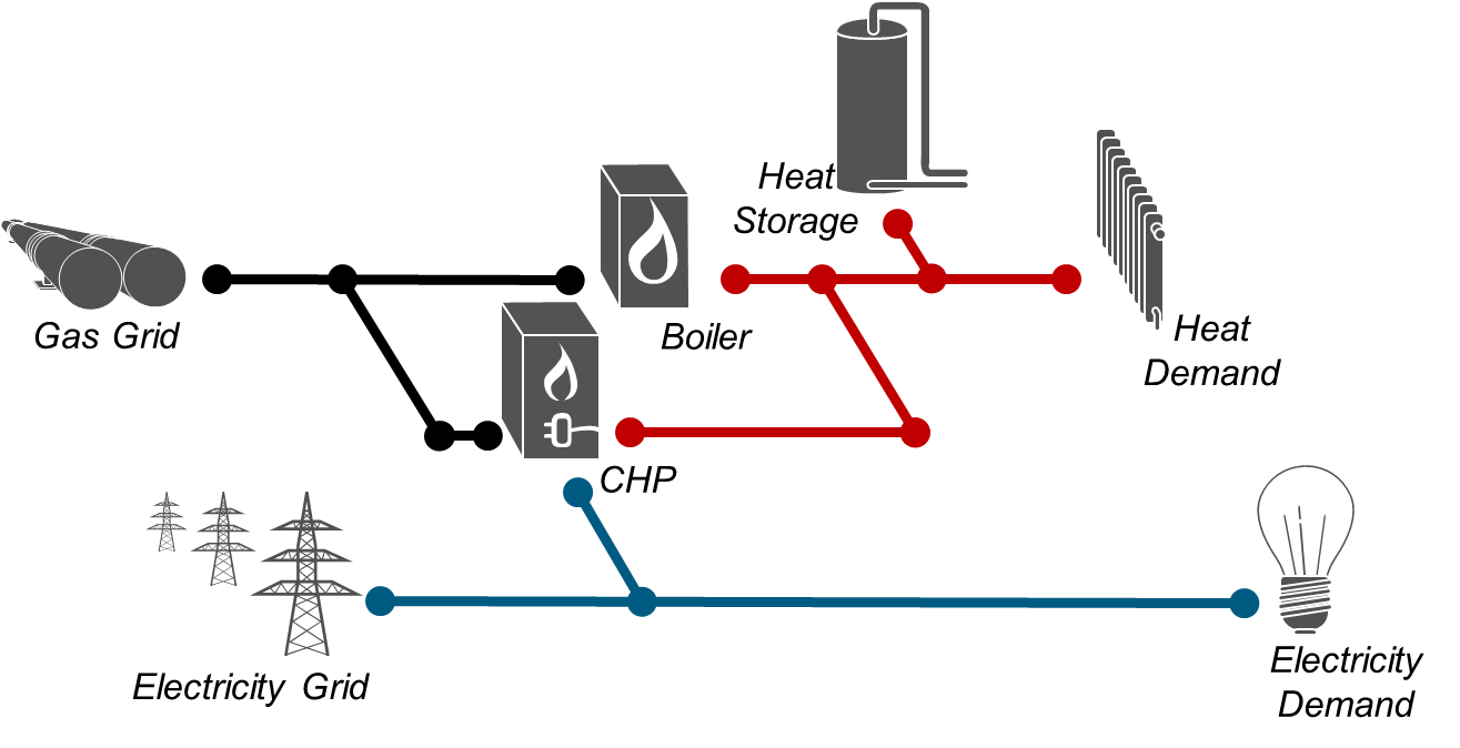
A combined heat and power plant (CHP) in combination with a gas boiler and heat storage for the supply of the residential electricity and heat demand, introduced in section 4.1.
- 2.
A residential supply system that is largely based on a heatpump and photovoltaics, introduced in section 4.2.
- 3.
An island system that supplies the electricity demand of an entire region, as introduced in section 4.3. This is based on photovoltaics and wind as power sources and also needs storage technologies because it has a limited access to fossil resources.
The aggregation methods and number of typical periods are varied and compared for all three systems. Furthermore, in the case of the residential system, we compare in detail the impact of different methods on integrating extreme periods. The island system is introduced to compare the impact of the varied length of the typical periods - e.g. typical days or typical weeks - on the system’s design.
The operation and design of the systems are optimized to achieve minimal costs of the energy supply. The general modeling approach of the systems is introduced in 0.A. The models are fairly simple in order to achieve a rapid solving performance in producing results for many different aggregation variants. The modeling language is Pyomo 4.3 [43] and as solver Gurobi 7.0.1 [44] was chosen. The hardware was an Intel i7-4790 CPU with 32 GB RAM, where 7 of 8 threads were used for solving.
4.1 CHP-based supply system
Optimizing the configuration and operation of a CHP system is a common application for typical period aggregation, especially if integer variables are included for choosing real components or modeling discrete states in the operation of the system. The CHP system is shown in Figure 11 and adds to the CHP itself a peak boiler and heat storage, which are all getting scaled and operated. The heat demand is simulated by a 5R1C model [34, 45], with the introduced weather data as an input for a multi-family house. The electrical load is aggregated by six single household profiles that Tjaden et al. [16] represent the housing units in the multi-family house.
4.1.1 Comparing the aggregation methods
For the validation, we optimized the system for the full original time series, and subsequently for different numbers of typical days, aggregated by the methods shown in section 2.2. The integration of peak periods was achieved by setting the days with the highest heat and highest electricity demand as additional cluster centers, which was discussed in section 2.3.
The results can be seen in Figure 12. It shows the relative error between the objective value, the annual cost, of the cost-optimal CHP system design based on aggregated periods, in comparison to the annual cost of the cost-optimal CHP system design based on the full time series for different types of aggregation methods. The bar plot is the composition of the annual cost of the optimal system design based on the full time series.
It is noticeable, that all aggregation methods underestimate the cost for a small number of typical periods, although the extreme periods are included. The reason for this is in the approach itself: The most representative periods are in general the days which have a smaller variance and smoother profiles than the original time series. The consequence is that the typical heat demand and the typical electricity demand fit better to each other, and the demand values do not exceed that often the capacity of the CHP plant. This results in an increased supply rates by the CHP system, with the consequence that for example the coverage with the CHP-plant is overestimated and the resulting system cost underestimated.
Therefore, it is also reasonable that the medoid based methods (k-medoids and hierarchical) perform better than the centroid based method k-mean. The choice of real days includes higher variations in comparison to an averaged profile as in the k-mean method. The averaging method performs, as expected, the worst because it is smoothing out to many fluctuations. No dominance of the hierarchical clustering or either the k-medoid clustering exists. For both methods it is possible to reach errors in the annual cost smaller than 2% with 8 typical days.
4.1.2 Gain in computational solving duration
The gain in the solving performance as a trade-off to the related accepted error is illustrated in Figure 13. As expected, the reduction in time steps results in a reduction of the solving time. The shape relates to the type of system model, while for our simple CHP-MILP we can consider a roughly logarithmic reduction of the error related to the solving performance. The precise shape depends on the scaling of the optimization problem and is not generalizable. Nevertheless, this pareto-front can be drawn for each system and it is up to the user to decide which degree of accuracy should be chosen. For the case of eight typical days, the solving time could get approximately reduced by a factor of 50 in solving based on the annual profile.
4.2 Residential supply system
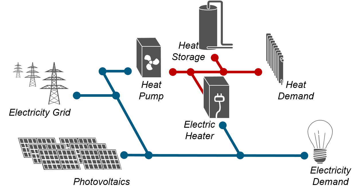
The second system analyzed is a supply system for a residential building based on a central grid supply and photovoltaics. The heat is supplied by a heat pump, an immersion heater with heat storage, as is seen in Figure 14. Heat and electricity loads are given for a single family house, while the photovoltaic feed-in profile is simulated in advance with the PV-Lib [46].
4.2.1 Comparing the aggregation methods
Like the CHP-system, different aggregation methods have been used for creating the typical periods, while varying also the number of typical days. The results are shown in Figure 15.
It is noticeable that the shape of the error functions of the residential systems are similar to the shape of the CHP system’s error function. Furthermore, for the residential system, k-mean clustering and averaging perform poorly in terms of underestimating the system cost, while the medoid based aggregation methods converge quickly on costs which are similar to the cost of the reference system, but overestimate the cost for higher numbers of typical days.
The high overestimates of the system cost of the hierarchical aggregation of three and four typical days show the sensitivity to the actual choice of representative days, e.g. a medoid day has a small overlay of the photovoltaic feed-in and electrical load profiles, self-supply rates are underestimated, with the effect that the energy cost are overestimated. These effects appear less with the k-mean aggregation because its profiles are averaged. Therefore, they converge more smoothly on smaller errors with an increased number of days.
The scale of the errors is in average twice as high as the error of the CHP systems for the same number of typical days. Therefore two factors must be taken into account:
- 1.
The electricity demand of a single household shows a higher fluctuation than that by an aggregated number of households, which is more difficult to capture in typical periods.
- 2.
An additional profile - the photovoltaic feed-in - impacts the optimal system design, which increases the number of patterns to collect with the aggregation methods.
Nevertheless, only 12 typical days are enough for reaching an error, corresponding to less than 2% of the objective value.
4.2.2 Comparing the integration of peak periods
In order to find the best method for the integration of peak periods, we applied all the methods introduced in section 2.3 to the residential system designed by six typical days aggregated by the k-medoid clustering. We manually defined for which time series, what type of peak period should be integrated:
- 1.
the day with peak heat load
- 2.
the day with peak electricity load
- 3.
the day with the smallest total photovoltaic feed-in
The results can be seen in Figure 16. If no extreme periods are integrated, the system costs are underestimated by roughly 2%. No improvement is recognizable apart from appending the peak periods. Setting the peak periods manually as a potential cluster center, the underestimation drops to 1%. The resulting design difference between these two integration methods is so small due to the fact that the peak periods are mostly at the edge of a cluster. In consequence, no or not many other observational periods are related to them. The last method, of replacing a whole cluster by a peak period, results in an overestimation of 3% and forces a more conservative system design because extreme periods are represented above average. A consequence of this is that the system design relies more on electricity supplied by the grid and less on photovoltaics as seen in Figure 17.
Also noteworthy is that for all the system designs derived from typical periods, the optimal photovoltaic capacity is overestimated, while the optimal storage capacities get underestimated. This is because of the already mentioned smoothing effect in the typical periods. The photovoltaic feed-in and electricity demand are predicted to be more steady, whereby a higher overlap exists. Furthermore, the heat demand is flattened, with less heat storage capacity required to balance it.
4.3 Island system
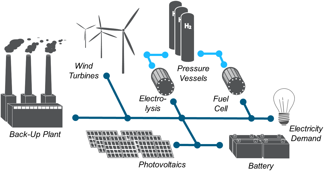
In terms of validating time series aggregation to a highly renewably based system design, we introduce an island system that is largely reliant on wind turbines and photovoltaics. The regional electricity demand profile and wind feed-in are drawn from Robinius et al. [42]. The potential photovoltaic feed-in is also simulated with PV-Lib [46]. A power plant gets scaled as backup capacity while its total feed-in is restricted to 10% of the total electricity demand, so as to achieve a high share of renewable energy supply. Furthermore, hydrogen storage based on electrolysers [47], fuel cells and pressure vessels, along with a battery storage can balance the fluctuating feed-in of the renewable time series. The entire system is shown in Figure 18.
4.3.1 Comparing the aggregation methods
As with both prior systems, the different aggregation methods and the number of typical days are first varied. The resulting optimal system design and errors are depicted in Figure 19.
The results in terms of the aggregation methods are the same as for both systems introduced previously. The major difference is the scale of the error: While the CHP system and the residential system both converged within less than 12 typical days to an error of less than 2% for the medoid-based aggregation methods, even for 72 typical days no robust convergence is identifiable for the island system.
As in the afore-mentioned systems, the smoothing-effect of the aggregation also partially contributes to the error, but therefore an underestimation of the resulting system cost would be expected. However, k-medoid and hierarchical clustering overestimate the system’s costs especially for high numbers of typical days.
Therefore, we expect the cause of the error to lie elsewhere: The cost optimal system design relies heavily on storage systems that contribute to almost 30% of the system costs, as is seen in Figure 19, including fuel cell, electrolyzer, hydrogen storage and battery. With the applied approach, each typical period is considered independently and no energy exchange between the typical periods is possible. For our case, this means that only storage operation within a single day is possible.
4.3.2 Variation of the period length
For this reason, we vary the duration of the typical periods. Along with the typical days (), typical groups of three days () and typical weeks () are also aggregated. We afix the aggregation methods to k-medoids and integrate the extreme periods as an additional cluster center.
Figure 20 shows the resulting error in the objective function and solving duration for the three different period lengths and different numbers of typical periods.
As was seen before, for typical days almost no convergence is recognizable.
The aggregation by groups of three days performs slightly better: With higher numbers of typical periods, the error gets reduced, but this convergence also appears non-monotonuously.
More predictable results can be achieved with typical weeks, which converge continuously on smaller errors. Nevertheless, the error also remains over 2% for 24 typical weeks. Furthermore, their solving performance is also worse due to the higher number of time steps per period.
For comparing aggregations with comparable solving performance, Figure 21 shows the cost composition for the aggregation of 21 typical days (each 24 time steps), seven typical periods based on three days (each 72 time steps) and three typical weeks (each 168 steps), which in sum have all the same number of time steps. They are compared to the original system design for validation.
The design based on the aggregation of typical days highly overestimates the capacities of renewable energies and battery storage required. In contrast to the original system design, the hydrogen storage is not integrated at all, as is seen in Figure 22. The same applies for the aggregation to typical groups of three days, which underestimates the overall system cost by 7%. Only in the case of the aggregation of typical weeks does a small hydrogen storage infrastructure gets built. All in all, this system design bears the highest degree of similarity to the original system, but also underestimates the costs by 9 %.
In summary, a poor performance of the typical period aggregation for the highly renewable based energy system design, including storages, can be identified. The cause of this is that the sequence of typical periods is not considered in the system model, with the consequence that long term storage cannot be properly taken into account.
5 Summary and discussion
Comparing the aggregation methods, the results show that averaging time series based on their appearance in the year, for example the average daily profile of a month, leads to an inaccurate system design.
As alternative aggregation methods, k-mean clustering, k-medoid clustering and hierarchical clustering have been compared for the creation of typical periods. In general, no aggregation method outperforms all the others for every case, but a trend is recognizable: The medoid, the most representative candidate period, performs better than the centroid, respectively an averaged time-series. The choice of the aggregation method itself, in this case k-medoid or hierarchical, has a fairly small influence.
The comparison of the aggregations of different time series indicates that solar irradiation, temperature and the electricity load of a whole region can be easily represented with a small error by means of the introduced aggregation methods. An electricity load of a single building is difficult to aggregate due to high fluctuation and the small daily pattern. Furthermore, wind data is challenging: The representative periods smooth out much of the original intra-period fluctuations. All aggregations were evaluated by so-called performance indicators, which have limited analytical value.
The methods have been further applied to three different system design optimizations: A CHP-based system, a residential system based on a heat pump and photovoltaics, and an island system with a high share of renewable energy. The outcome shows that the impact of the time series aggregation is significantly reliant on the structure of the energy system itself.
The best results could be achieved for the CHP and the residential system, which are highly dependent on central supply infrastructures – either gas imports, which would also hold for other fuel imports, or a connection to the electricity grid. Therefore, a total of eight to twelve typical days was sufficient to reach cost prediction errors less than 2% while reducing the solving duration of the optimization problem by a factor of 50 in comparison to using the time series of a full year.
For the case of the island system, the current modeling approach leads to high estimation errors. The optimization based on the aggregated periods caused a modeling error because the typical periods are independent and cannot exchange energy. Therefore, storage technologies were not properly taken into account. An extension from typical days to typical weeks brought about a small improvement but was, as expected, still unable to account for seasonal storage.
6 Conclusion
This paper investigated the effect of time series aggregation on optimal energy system design models. We showed that a time series aggregation based on clustering algorithms can significantly reduce model complexity and the required computational time.
Comparing different aggregation methods, the results indicate that the choice of the aggregation algorithm itself has only a minor impact on the optimal system design. Nevertheless, the authors would recommend a hierarchical aggregation due to its small computational load and reproducibility. The choice of the representative periods from the aggregated clusters is of more relevance; cluster medoids, i.e., using real periods, produced more accurate results than k-mean centroids, which use averaged periods.
A qualitative analysis using aggregated time series samples showed that the series representing entire regions can be more easily aggregated than those for single locations, i.e., less typical periods, can be sufficiently representative. Hence, aggregation methods are expected to be more valuable for spatially-aggregated systems than for models with finer resolution.
Furthermore, we illustrate that the trade-off between the depth of time series reduction and the resulting modeling error depends highly on the system configuration. While energy systems based on centralized supply resources can be well represented with a few typical days, energy systems heavily relying on storage technologies cannot be properly represented by independent typical days at all, nor by independent typical weeks.
This leads to the conclusion that the impact of applying time series aggregation methods must be evaluated separately for each energy system model, or at least for a simplified model version. Merely assessing the aggregated time series by performance indicators can lead to significant deviation from an optimal design.
7 Outlook
Based on the conclusion, new modeling methods are required that take the sequence of the aggregated typical periods into account, with the objective of modeling the operation of long term storage contingencies.
Furthermore, future research should identify more cluster-relevant parameters like gradients and variance, etc., because the current clustering leads to smoothed typical periods that underestimate the variability of the original time series.
All methods introduced are published in the Python package tsam - Time Series Aggregation Module and can be easily applied and extended.
Acknowledgments
This work was supported by the Helmholtz Association under the Joint Initiative "EnergySystem 2050 – A Contribution of the Research Field Energy".
Appendix 0.A System modeling
For validation purposes, a comprehensible simple Mixed-Integer Linear Program has been chosen as the system model. This is defined by a network of specific technologies that are connected by energy flow variables at time step . Each connection is therefore defined by an output component and input component and belongs to a connection set . These connections are restricted by the introduced component models.
For a typical period, the time steps are replaced by the time steps within a single period .
0.A.1 Objective function
The objective function describes the annualized cost of the supply system considered. Therefore, for each device , the annualized cost are calculated with a capital recovery factor , which considers the Weighted Average Cost of Capital and lifetime of the device in years:
| (14) |
The capital expenditure of each component is divided into the existing related costs [eur], which only appear if the component is installed, and scale related costs [eur/kW], specific costs, which are scale dependent [48]. For this reason, each component is modeled by a binary variable that defines whether the component exists, and a continuous variable , which defines the installed capacity of the component. The resulting device specific annualized fixed cost can be calculated with the existing related capital expenditure (), the scaling-related capital expenditure () and fixed operational expenditure () as follows
The costs that variate with the operation of the system are related to the energy flows . Along with the scaling of the devices , the following objective function can be stated:
| (17) |
0.A.2 Constraints
The device models establish the constraints of the system. They are divided into five classes: Source/Sinks, Collectors, Transformers and Storages.
The Source/Sink class represents input and output flows to the system, like photovoltaic feed-in or electricity demand. It is essentially defined by a single equation:
| (18) |
where could be a certain demand that must at least be satisfied at timestep , or could be the maximal photovoltaic feed-in per installed capacity.
The Collectors class can be seen as a hub where all input energy flows must be equivalent to all output energy flows:
| (19) |
The Transformer class represents devices that transform the energy from one form to another. Examples are a fuel cells or heat pumps. For their definition, the energy type (electricity, gas, etc.) must be introduced. Each energy flow has a certain energy type . With the energy type specific transformation efficiency , the following equation can be stated for each energy transformation in the device:
| (20) |
The Storage class is defined by an additional variable the State of Charge at time step . We can utilize the Euler method to state for the state of charge in the next time step :
| (21) |
where describes the charging flow with an efficiency of and the discharging flow with related efficiency . defines the self-discharge of the storage and the step length of a single time step. The state of charge at the beginning of the considered time frame is related to that in the end of the time frame .
The design variable of the storage which is described by its capacity limits the state of charge to the following:
| (22) |
The existing related variable restricts the scaling-dependent device variable by the so called BigM-Method [49] as follows:
| (23) |
The method is inspired by Stadler et al. [3] and Lindberg et al. [48].
References
References
- [1] R. Baños, F. Manzano-Agugliaro, F. G. Montoya, C. Gil, A. Alcayde, J. Gómez, Optimization methods applied to renewable and sustainable energy: A review, Renewable and Sustainable Energy Reviews 15 (4) (2011) 1753–1766, ISSN 13640321, doi:10.1016/j.rser.2010.12.008.
- [2] P. Petruschke, G. Gasparovic, P. Voll, G. Krajačić, N. Duić, A. Bardow, A hybrid approach for the efficient synthesis of renewable energy systems, Applied Energy 135 (2014) 625–633, ISSN 03062619, doi:10.1016/j.apenergy.2014.03.051.
- [3] M. Stadler, M. Groissböck, G. Cardoso, C. Marnay, Optimizing Distributed Energy Resources and building retrofits with the strategic DER-CAModel, Applied Energy 132 (2014) 557–567, ISSN 03062619, doi:10.1016/j.apenergy.2014.07.041.
- [4] S. Kwon, W. Won, J. Kim, A superstructure model of an isolated power supply system using renewable energy: Development and application to Jeju Island, Korea, Renewable Energy 97 (2016) 177–188, ISSN 09601481, doi:10.1016/j.renene.2016.05.074.
- [5] S. Samsatli, N. J. Samsatli, A general spatio-temporal model of energy systems with a detailed account of transport and storage, Computers & Chemical Engineering 80 (2015) 155–176, ISSN 00981354, doi:10.1016/j.compchemeng.2015.05.019.
- [6] E. Merkel, R. McKenna, W. Fichtner, Optimisation of the capacity and the dispatch of decentralised micro-CHP systems: A case study for the UK, Applied Energy 140 (2015) 120–134, ISSN 03062619, doi:10.1016/j.apenergy.2014.11.036.
- [7] C. Milan, C. Bojesen, M. P. Nielsen, A cost optimization model for 100% renewable residential energy supply systems, Energy 48 (1) (2012) 118–127, ISSN 03605442, doi:10.1016/j.energy.2012.05.034.
- [8] D. Lauinger, P. Caliandro, J. Van herle, D. Kuhn, A linear programming approach to the optimization of residential energy systems, Journal of Energy Storage 7 (2016) 24–37, ISSN 2352152X, doi:10.1016/j.est.2016.04.009.
- [9] G. Merei, J. Moshövel, D. Magnor, D. U. Sauer, Optimization of self-consumption and techno-economic analysis of PV-battery systems in commercial applications, Applied Energy 168 (2016) 171–178, ISSN 03062619, doi:10.1016/j.apenergy.2016.01.083.
- [10] H. Wang, W. Yin, E. Abdollahi, R. Lahdelma, W. Jiao, Modelling and optimization of CHP based district heating system with renewable energy production and energy storage, Applied Energy 159 (2015) 401–421, ISSN 03062619, doi:10.1016/j.apenergy.2015.09.020.
- [11] A. Palzer, H.-M. Henning, A comprehensive model for the German electricity and heat sector in a future energy system with a dominant contribution from renewable energy technologies –Part II: Results, Renewable and Sustainable Energy Reviews 30 (2014) 1019–1034, ISSN 13640321, doi:10.1016/j.rser.2013.11.032.
- [12] P. Mancarella, MES (multi-energy systems): An overview of concepts and evaluation models, Energy 65 (2014) 1–17, ISSN 03605442, doi:10.1016/j.energy.2013.10.041.
- [13] M. Geidl, G. Andersson, Optimal Power Flow of Multiple Energy Carriers, IEEE Transactions on Power Systems 22 (1) (2007) 145–155, ISSN 0885-8950, doi:10.1109/tpwrs.2006.888988.
- [14] C. Milan, M. Stadler, G. Cardoso, S. Mashayekh, Modeling of non-linear CHP efficiency curves in distributed energy systems, Applied Energy 148 (2015) 334–347, ISSN 03062619, doi:10.1016/j.apenergy.2015.03.053.
- [15] DWD, Testreferenzjahre (TRY) .
- [16] T. Tjaden, J. Bergner, J. Weniger, V. Quaschning, Repraesentative elektrische Lastprofile fuer Wohngebaeude in Deutschland auf 1-sekuendiger Datenbasis doi:10.13140/RG.2.1.5112.0080.
- [17] C. Golling, A cost-efficient expansion of renewable energy sources in the European electricity system - an integrated modelling approach with a particular emphasis on diurnal and seasonal patterns, Thesis, URL http://kups.ub.uni-koeln.de/4856/, 2012.
- [18] K. Poncelet, H. Höschle, E. Delarue, A. Virag, W. D’ haeseleer, Selecting representative days for capturing the implications of integrating intermittend renewables in generation expansion planning problems, IEE Transaction on Power Systems URL http://ieeexplore.ieee.org/stamp/stamp.jsp?arnumber=7527691.
- [19] J. Ortiga, J. C. Bruno, A. Coronas, Selection of typical days for the characterisation of energy demand in cogeneration and trigeneration optimisation models for buildings, Energy Conversion and Management 52 (4) (2011) 1934–1942, ISSN 01968904, doi:10.1016/j.enconman.2010.11.022.
- [20] G. Mavrotas, D. Diakoulaki, K. Florios, P. Georgiou, A mathematical programming framework for energy planning in services’ sector buildings under uncertainty in load demand: The case of a hospital in Athens, Energy Policy 36 (7) (2008) 2415–2429, ISSN 03014215, doi:10.1016/j.enpol.2008.01.011.
- [21] E. D. Mehleri, H. Sarimveis, N. C. Markatos, L. G. Papageorgiou, Optimal design and operation of distributed energy systems: Application to Greek residential sector, Renewable Energy 51 (2013) 331–342, ISSN 09601481, doi:10.1016/j.renene.2012.09.009.
- [22] M. Casisi, P. Pinamonti, M. Reini, Optimal lay-out and operation of combined heat & power (CHP) distributed generation systems, Energy 34 (12) (2009) 2175–2183, ISSN 03605442, doi:10.1016/j.energy.2008.10.019.
- [23] M. A. Lozano, J. C. Ramos, M. Carvalho, L. M. Serra, Structure optimization of energy supply systems in tertiary sector buildings, Energy and Buildings 41 (10) (2009) 1063–1075, ISSN 03787788, doi:10.1016/j.enbuild.2009.05.008.
- [24] C. E. Lythcke-Jørgensen, M. Münster, A. V. Ensinas, F. Haglind, A method for aggregating external operating conditions in multi-generation system optimization models, Applied Energy 166 (2016) 59–75, ISSN 03062619, doi:10.1016/j.apenergy.2015.12.050.
- [25] S. P. Adhau, R. M. Moharil, P. G. Adhau, K-Means clustering technique applied to availability of micro hydro power, Sustainable Energy Technologies and Assessments 8 (2014) 191–201, ISSN 22131388, doi:10.1016/j.seta.2014.09.001.
- [26] R. Green, I. Staffell, N. Vasilakos, Divide and Conquer - Means Clustering of Demand Data Allows Rapid and Accurate Simulations of the British Electricity System, IEEE Transactions on Engineering Management 61 (2) (2014) 251–260, ISSN 0018-9391 1558-0040, doi:10.1109/tem.2013.2284386.
- [27] B. Bahl, A. Kuempel, M. Lampe, A. Bardow, Time-series aggregation for synthesis of distributed energy supply systems by bounding error in operational expenditure, in: Z. Kravanja (Ed.), 26th European Symposium on Computer Aided Process Engineering, Elsevier B.V, 2016.
- [28] S. Fazlollahi, S. L. Bungener, P. Mandel, G. Becker, F. Maréchal, Multi-objectives, multi-period optimization of district energy systems: I. Selection of typical operating periods, Computers & Chemical Engineering 65 (2014a) 54–66, ISSN 00981354, doi:10.1016/j.compchemeng.2014.03.005.
- [29] J. H. Merrick, On representation of temporal variability in electricity capacity planning models, Energy Economics 59 (2016) 261–274, ISSN 01409883, doi:10.1016/j.eneco.2016.08.001.
- [30] P. Nahmmacher, E. Schmid, L. Hirth, B. Knopf, Carpe diem: A novel approach to select representative days for long-term power system modeling, Energy 112 (2016) 430–442, ISSN 03605442, doi:10.1016/j.energy.2016.06.081.
- [31] J. M. F. Rager, F. Maréchal, Urban Energy System Design from the Heat Perspective using mathematical Programming including thermal Storage, Thesis, doi:10.5075/epfl-thesis-6731, 2015.
- [32] P. Stadler, A. Ashouri, F. Maréchal, Model-based optimization of distributed and renewable energy systems in buildings, Energy and Buildings 120 (2016) 103–113, ISSN 03787788, doi:10.1016/j.enbuild.2016.03.051.
- [33] F. Domínguez-Muñoz, J. M. Cejudo-López, A. Carrillo-Andrés, M. Gallardo-Salazar, Selection of typical demand days for CHP optimization, Energy and Buildings 43 (11) (2011) 3036–3043, ISSN 03787788, doi:10.1016/j.enbuild.2011.07.024.
- [34] T. Schuetz, L. Schiffer, H. Harb, M. Fuchs, D. Müller, Optimal design of energy conversion units and envelopes for residential building retrofits using a comprehensive MILP model, Applied Energy 185 (2017) 1–15, ISSN 03062619, doi:10.1016/j.apenergy.2016.10.049.
- [35] T. Schuetz, M. H. Schraven, H. Harb, M. Fuchs, D. Müller, Clustering algorithms for the selection of typical demand days for the optimal design of building energy systems, in: Efficiency, Cost, Optimization, Simulation and Environmental Impact of Energy Systems, 2016.
- [36] K. Poncelet, E. Delarue, J. Duerinck, D. Six, W. D’haeseleer, The importance of integrating the variability of renewables in long-term energy planning models, Report, KU Leuven, URL https://www.mech.kuleuven.be/en/tme/research/energy_environment/Pdf/wp-importance.pdf, 2014.
- [37] H. Harb, C. Schwager, R. Streblow, D. Müller, Optimal Design of Energy Systems in Residential Districts with Interconnected Local Heating and Electrical Networks, in: Building Simulation Conference, doi:10.13140/RG.2.1.2144.6488, 2015.
- [38] A. K. Jain, Data clustering: 50 years beyond K-means, Pattern Recognition Letters 31 (8) (2010) 651–666, ISSN 01678655, doi:10.1016/j.patrec.2009.09.011.
- [39] S. Fazlollahi, G. Becker, F. Maréchal, Multi-objectives, multi-period optimization of district energy systems: II-Daily thermal storage, Computers & Chemical Engineering 71 (2014b) 648–662, ISSN 00981354, doi:10.1016/j.compchemeng.2013.10.016.
- [40] A. P. Reynolds, G. Richards, B. D. L. Iglesia, V. J. Rayward-Smith, Clustering Rules: A Comparison of Partitioning and Hierarchical Clustering Algorithms, Journal of Mathematical Modelling and Algorithms 5 (2006) 475–504, URL http://link.springer.com/article/10.1007/s10852-005-9022-1.
- [41] M. Robinius, Strom- und Gasmarktdesign zur Versorgung des deutschen Straßenverkehrs mit Wasserstoff, Thesis, 2015.
- [42] M. Robinius, F. t. Stein, A. Schwane, D. Stolten, A Top-Down Spatially Resolved Electrical Load Model, Energies 10 (3) (2017) 361, ISSN 1996-1073, doi:10.3390/en10030361.
- [43] W. E. Hart, C. Laird, D. L. Woodruff, Pyomo: modeling and solving mathematical programs in Python, Mathematical Programming Computation 3 (3) (2011) 219–260.
- [44] I. Gurobi Optimization, Gurobi Optimizer Reference Manual, URL http://www.gurobi.com, 2016.
- [45] D. EN ISO, Thermal performance and energy use in the build environment (ISO 13790:2008) .
- [46] R. W. Andrews, J. S. Stein, C. Hansen, D. Riley, Introduction to the Open Source PV-LIB for Python Photovoltaic System Modeling Package .
- [47] S. Schiebahn, T. Grube, M. Robinius, V. Tietze, B. Kumar, D. Stolten, Power to gas: Technological overview, systems analysis and economic assessment for a case study in Germany, International Journal of Hydrogen Energy 40 (12) (2015) 4285–4294, ISSN 03603199, doi:10.1016/j.ijhydene.2015.01.123.
- [48] K. B. Lindberg, G. Doorman, D. Fischer, M. Korpås, A. Ånestad, I. Sartori, Methodology for optimal energy system design of Zero Energy Buildings using mixed-integer linear programming, Energy and Buildings 127 (2016) 194–205, ISSN 03787788, doi:10.1016/j.enbuild.2016.05.039.
- [49] A. Bemporad, M. Morari, Control of systems integrating logic, dynamics, and constraints, Automatica 35 (3) (1999) 407–427, ISSN 0005-1098, doi:Doi 10.1016/S0005-1098(98)00178-2, URL <GotoISI>://WOS:000079457800006.