跳到论文正文
W Papers独立论文阅读器 arXiv:1708.00205 论文正文 计算阅读时间 · 0%
引用这篇论文根据当前论文元数据生成,正式投稿前建议核对。


License: arXiv.org perpetual non-exclusive license
arXiv:1708.00205v3 [stat.ME] 18 Jan 2019

Dynamic Linear Discriminant Analysis in High Dimensional Space

Binyan Jiang    Ziqi Chen    Chenlei Leng Note: Jiang is with the Hong Kong Polytechnic University. Chen is with Central South University. Leng is with the University of Warwick.
Abstract

High-dimensional data that evolve dynamically feature predominantly in the modern data era. As a partial response to this, recent years have seen increasing emphasis to address the dimensionality challenge. However, the non-static nature of these datasets is largely ignored. This paper addresses both challenges by proposing a novel yet simple dynamic linear programming discriminant (DLPD) rule for binary classification. Different from the usual static linear discriminant analysis, the new method is able to capture the changing distributions of the underlying populations by modeling their means and covariances as smooth functions of covariates of interest. Under an approximate sparse condition, we show that the conditional misclassification rate of the DLPD rule converges to the Bayes risk in probability uniformly over the range of the variables used for modeling the dynamics, when the dimensionality is allowed to grow exponentially with the sample size. The minimax lower bound of the estimation of the Bayes risk is also established, implying that the misclassification rate of our proposed rule is minimax-rate optimal. The promising performance of the DLPD rule is illustrated via extensive simulation studies and the analysis of a breast cancer dataset.

Key Words: Bayes rule; Discriminant analysis; Dynamic linear programming; High-dimensional data; Kernel smoothing; Sparsity.

1 Introduction

The rapid development of modern measurement technologies has enabled us to gather data that are increasingly larger. As the rule rather than the exception, these datasets have been gathered at different time, under different conditions, subject to a variety of perturbations, and so on. As a result, the complexity of many modern data is predominantly characterized by high dimensionality and the data dynamics. The former is featured by a large number of variables in comparison to the sample size, and the manifestation of the latter can be seen in the distribution of the data which is non-static and dependent on covariates such as time. Any approach ignoring either of the two aspects may give unsatisfactory performance and even incorrect conclusions.

The main aim of this paper is to address these two challenges simultaneously, for the first time, by developing a very simple yet useful dynamic linear programming discriminant (DLPD) rule for classification. Specializing to binary classification, we allow the means and the covariance matrices of the populations to vary with covariates of interest, which are estimated via local smoothing (Fan & Gijbels, 1996). Under an approximate sparsity assumption on a linear index that is central to classification, we propose to estimate the index vector via a technique akin to the Dantzig selector (Candes & Tao, 2007; Cai & Liu, 2011) in a dynamic setting. We show emphatically that the conditional misclassification rate of the DLPD rule converges to the Bayes risk in probability uniformly over a range of the variables used for modeling dynamics, where the dimensionality is allowed to be exponentially high relative to the sample size. The uniformity result is of particular importance as it permits simultaneous statements over the whole range of the covariate. In addition, we derived minimax lower bounds for the Bayes risk, which indicates that the misclassification rate of our DLPD rule is minimax-rate optimal. To our best knowledge, this is the first attempt in developing a high-dimensional discriminant method that exhibits local features of the data with sound theory. We remark that using existing approaches such as the one in Cai & Liu (2011) coupled with local smoothing, it is possible to establish a pointwise result for the misclassification rate. However, a pointwise convergence result will not be sufficient in a dynamic setting, as the main interest is often to assess the estimated classification rule across the whole of the covariates, not just at a single point of the covariates.

Before we proceed further, let’s quickly look at a dataset that motivated this study. In traditional disease diagnosis studies, the same classification rule for all the patients was often applied. However, it has become increasingly more desirable to develop personalized rules that takes into account individual characteristics (Alyass, Turcotte & Meyre, 2015). Intuitively, these patient-specific factors can be treated as dynamic factors in deriving decision rules. For example, in the breast cancer data we studied in Section 4.3, both (low dimensional) clinical risk factors (tumor size, age, histological grade etc.) and (high dimensional) expression levels for 24,481 gene probes were collected for 97 lymph node-negative breast cancer patients. Among them, 46 patients developed distant metastases within 5 years while the rest 51 remained metastases free for at least 5 years. To appreciate the need to incorporate dynamic information into the analysis, we look at the 100 genes with the largest absolute tt-statistic values between the two groups choosing the tumor size as the dynamic variable. We fit the gene expression levels as a function of the tumor size using a local regression model (Cleveland, Grosse & Shyu, 1992). The fitted plots for some randomly selected genes are presented in Figure 1, from which we can see that the gene expression levels of the patients in the two classes exhibit different levels as the tumor size changes. Similarly, the covariance matrix of these 100 genes also is found to behave dynamically in response to the changes of the tumor size. To see this, we separate the 97 observations into two groups depending on whether the tumor size is greater than the median of the tumor sizes 2.485. A pp-value <0.001<0.001 (Li & Chen, 2011) indicates that we should reject the null hypothesis that the population covariance matrices of the two groups are equal. The method developed in this paper aims to capture this dynamic information in a high-dimensional setting for classification.

Figure 1: Gene expression level versus tumor size. Upper panel: selected genes from XX class; Lower panel: selected genes from YY class. The curves are LOWESS fits.

1.1 The setup

We now introduce formally the problem. Let X=(x1,…CLOSE,X=(x_{1},\ldots, OPENxp)Tx_{p})^{T}, Y=(y1,…,yp)TY=(y_{1},\ldots,y_{p})^{T} be pp-dimensional random vectors and 𝐔{\bf U} be a dd-dimensional random covariate, where for simplicity we assume that dd is a fixed integer. In this paper we deal with the situation where pp is large. Given 𝐔{\bf U} we assume that X∼N⁡(μX​(𝐔),Σ⁡(𝐔))X\sim N(\mu_{X}({\bf U}),\Sigma({\bf U})) where μX​(𝐔)=(μX1​(𝐔),…,μXp​(𝐔))T\mu_{X}({\bf U})=(\mu_{X}^{1}({\bf U}),\ldots,\mu_{X}^{p}({\bf U}))^{T} and Σ⁡(𝐔)=(σi​j​(𝐔))1≤i,j≤p\Sigma({\bf{\bf U}})=(\sigma_{ij}({\bf U}))_{1\leq i,j\leq p}. Similarly, the conditional distribution of YY given 𝐔{\bf U} is given as Y∼N⁡(μY​(𝐔),Σ⁡(𝐔))Y\sim N(\mu_{Y}({\bf U}),\Sigma({\bf U})) where μY​(𝐔)=(μY1​(𝐔),…,μYp​(𝐔))T\mu_{Y}({\bf U})=(\mu_{Y}^{1}({\bf U}),\ldots,\mu_{Y}^{p}({\bf U}))^{T}. In other words, different from traditional linear discriminant analysis, we assume that the first and second moments of XX and YY change over a dd-dimensional covariate 𝐔{\bf U}. Here 𝐔{\bf U} could be dependent on the features XX and YY. When 𝐔{\bf U} is a vector of discrete variables, the above mentioned model is named the location-scale model and was used for discriminant analysis with mixed data under finite dimension assumptions; see, for example, Krzanowski (1993) and the references therein.

In discriminant analysis, it is well known that the Bayes procedure is admissible; see for example Anderson (2003). Let (Z,𝐔Z)(Z,{\bf U}_{Z}) be a generic random sample which can be from either the population (X;𝐔)(X;{\bf U}) or the population (Y;𝐔)(Y;{\bf U}). In this paper we assume a priori that it is equally likely that (Z,𝐔Z)(Z,{\bf U}_{Z}) comes from either population (X;𝐔)(X;{\bf U}) or population (Y;𝐔)(Y;{\bf U}). Following simple algebra, it can be easily shown that the Bayes procedure is given as the following:

  • (i)

    Classify (Z,𝐔Z)(Z,{\bf U}_{Z}) into population (X,𝐔)(X,{\bf U}) if

    {Z−[μX​(𝐔Z)+μY​(𝐔Z)]/2}T​Σ−1​(𝐔Z)​[μX​(𝐔Z)−μY​(𝐔Z)]≥0;\{Z-[\mu_{X}({\bf U}_{Z})+\mu_{Y}({\bf U}_{Z})]/2\}^{T}\Sigma^{-1}({\bf U}_{Z})[\mu_{X}({\bf U}_{Z})-\mu_{Y}({\bf U}_{Z})]\geq 0;
  • (ii)

    Classify (Z,𝐔Z)(Z,{\bf U}_{Z}) into population (Y,𝐔)(Y,{\bf U}) otherwise.

Given 𝐔z=𝐮{\bf U}_{z}={\bf u}, by standard calculation, the conditional misclassification rate of this rule is

R(𝐮)=Φ(−Δp(𝐮)/2),\displaystyle R({\bf u})=\Phi(-\Delta_{p}({\bf u})/2), (1)

where Δp​(𝐮)=[μX​(𝐮)−μY​(𝐮)]T​Σ−1​(𝐮)​[μX​(𝐮)−μY​(𝐮)],\Delta_{p}({\bf u})=\sqrt{[\mu_{X}({\bf u})-\mu_{Y}({\bf u})]^{T}\Sigma^{-1}({\bf u})[\mu_{X}({\bf u})-\mu_{Y}({\bf u})]}, and Φ⁡(⋅)\Phi(\cdot) is the cumulative distribution function of a standard normal random variable. The expected misclassification rate is defined as

R=E𝐔​R​(𝐔),\displaystyle R={\rm E}_{\bf U}R({\bf U}), (2)

where E𝐔{\rm E}_{\bf U} means taking expectation with respect to 𝐔{\bf U}. Practically μX​(⋅)\mu_{X}(\cdot), μY​(⋅)\mu_{Y}(\cdot) and Σ⁡(⋅)\Sigma(\cdot) are unknown but there are a sequence of independent random observations (Xi,𝐔i)(X_{i},{\bf U}_{i}), i=1,…,n1i=1,\ldots,n_{1} from the population (X;𝐔)(X;{\bf U}) and a sequence of independent random observations (Yj,𝐕j)(Y_{j},{\bf V}_{j}), j=1​…,n2j=1\ldots,n_{2} from the population (Y,𝐔)(Y,{\bf U}). The central problem then becomes proposing methods based on the sample that give misclassification rates converging to that of the Bayes rule under appropriate assumptions.

1.2 Existing works

There has been increasing emphasis in recent years to address the high-dimensionality challenge posed by modern data where pp is large. However, the dynamic nature of the data collection process is often ignored in that μ⁡(𝐔)\mu({\bf U}) and Σ⁡(𝐔)\Sigma({\bf U}) are assumed to be independent of 𝐔{\bf U}. In this static case, the Bayes procedure given above reduces to the well-known Fisher’s linear discriminant analysis (LDA). In static high dimensional discriminant analysis, Bickel & Levina (2004) first highlighted that Fisher’s LDA is equivalent to random guessing. Fortunately, in many problems, various quantities in the LDA can be assumed sparse; See, for example, Witten & Tibshirani (2011); Shao et al. (2011); Cai & Liu (2011); Fan, Feng & Tong (2012); Mai, Zou & Yuan (2012), and Mai & Zou (2013) for a summary of selected sparse LDA methods. Further studies along this line can be found in Fan, Jin & Yao (2013) and Hao, Dong & Fan (2015). More recently, quadratic discriminant analysis has attracted increasing attention where the population covariance matrices are assumed static but different. This has motivated the study of more flexible models exploiting variable interactions for classification, analogous to two-way interaction in linear regression; see for example Fan, Ke & Liu (2015), Fan, et al. (2015), and Jiang:etal:2015. However, none of these works addresses the dynamic nature of μ⁡(⋅)\mu(\cdot) and Σ⁡(⋅)\Sigma(\cdot).

In our setup where dynamics exists, in addition to the high dimensionality, we need to obtain dynamic estimators for μX​(𝐮)−μY​(𝐮)\mu_{X}({\bf u})-\mu_{Y}({\bf u}) and Σ−1​(𝐮)\Sigma^{-1}({\bf u}), or

β⁡(𝐮):=Σ−1​(𝐮)​[μX​(𝐮)−μY​(𝐮)]\beta({\bf u}):=\Sigma^{-1}({\bf u})[\mu_{X}({\bf u})-\mu_{Y}({\bf u})]

as functions of 𝐮{\bf u}. Under a similar setup where 𝐔{\bf U} is categorical and supported on a set of finite elements, Guo et al. (2011) proposed a sparse estimator for Σ−1​(𝐮)\Sigma^{-1}({\bf u}). The emphasis of this work is for continuous 𝐔{\bf U} that is compactly supported. Chen & Leng (2015) proposed nonparametric estimators of sparse Σ⁡(𝐮)\Sigma({\bf u}) using thresholding techniques for univariate 𝐔{\bf U} where d=1d=1. The focus of this paper on high-dimensional classification is completely different. Importantly, we do not require the sparsity assumption on Σ⁡(𝐮)\Sigma({\bf u}) and our theory applies for any fixed-dimensional 𝐔{\bf U}. Our paper is also different from Cai & Liu (2011), Fan, Feng & Tong (2012) and Mai, Zou & Yuan (2012) in that β⁡(𝐮)\beta(\bf u) is allowed not only to be a smooth function of 𝐔{\bf U}, but also to be approximately sparse (see Theorem 1). Our efforts greatly advance the now-classical approach of local polynomial (Fan & Gijbels, 1996) to the modern era of high-dimensional data analysis.

If we denote μ^X​(𝐔Z),μ^Y​(𝐔Z)\hat{\mu}_{X}({\bf U}_{Z}),\hat{\mu}_{Y}({\bf U}_{Z}) and β^​(𝐔Z)\hat{\beta}({\bf U}_{Z}) as the estimators of μX​(𝐔Z)\mu_{X}({\bf U}_{Z}), μY​(𝐔Z)\mu_{Y}({\bf U}_{Z}) and β⁡(𝐔Z)\beta({\bf U}_{Z}) defined as in Section 2 respectively, our Dynamic Linear Programming Discriminant (DLPD) rule is given as the following:

  • (i)

    Classify (Z,𝐔Z)(Z,{\bf U}_{Z}) into population (X,𝐔)(X,{\bf U}) if:

    {Z−[μ^X​(𝐔Z)+μ^Y​(𝐔Z)]/2}T​β^​(𝐔Z)≥0;\{Z-[\hat{\mu}_{X}({\bf U}_{Z})+\hat{\mu}_{Y}({\bf U}_{Z})]/2\}^{T}\hat{\beta}({\bf U}_{Z})\geq 0;
  • (ii)

    Classify (Z,𝐔Z)(Z,{\bf U}_{Z}) into population (Y,𝐔)(Y,{\bf U}) otherwise.

The rest of this paper is organized as follows. In Section 2, we propose estimators for the components in the Bayes rule and propose the DLPD rule. Section 3 provides theoretical results of our DLPD rule. In particular, we show that under appropriate conditions, the risk function of the DLPD rule converges to the Bayes risk function uniformly in 𝐮{\bf u}. In addition, we derived minimax lower bounds for the estimation of Δ⁡(𝐮)\Delta({\bf u}) and the Bayes risk. In section 4, simulation study is conducted to assess the finite sample performance of the proposal method. The DLPD rule is then applied to solve interesting discriminant problems using a breast cancer dataset. Concluding remarks are made in Section 5. All the theoretical proofs are given in the Appendix.

2 A dynamic linear programming discriminant rule

We begin by introducing some notations. For any matrix MM, we use MTM^{T}, |M||M| and tr⁡(M){\rm tr}(M) to denote its transpose, determinant and trace. Let v=(v1,…,vp)T∈ℛpv=(v_{1},\ldots,v_{p})^{T}\in\mathcal{R}^{p} be a pp-dimensional vector. Define |v|0=∑i=1pI{vi≠0}|v|_{0}=\sum_{i=1}^{p}I_{\{v_{i}\neq 0\}} as the ℓ0\ell_{0} norm and |v|∞=max1≤i≤p⁡|vi||v|_{\infty}=\max_{1\leq i\leq p}|v_{i}| as the ℓ∞\ell_{\infty} norm. For any 1≤q<∞1\leq q<\infty, the lql_{q} norm of vv is defined as |v|q=(∑i=1p|vi|q)1/q|v|_{q}=(\sum_{i=1}^{p}|v_{i}|^{q})^{1/q}. We denote the pp-dimensional vector of ones as 1p1_{p} and the pp-dimensional vector of zeros as 0p0_{p}.

Denote 𝐮=(u1,…,ud)T{\bf u}=(u_{1},\ldots,u_{d})^{T} and let 𝐊⁡(𝐮){\bf K}({\bf u}) be a kernel function such that

𝐊(𝐮)=Πi=1dK(u1)×⋯×K(ud),\displaystyle{\bf K}({\bf u})=\Pi_{i=1}^{d}K(u_{1})\times\cdots\times K(u_{d}),

where K⁡(⋅)K(\cdot) is an univariate kernel function, for example, the Epanechnikov kernel used in kernel smoothing (Fan & Gijbels, 1996). Recent literature on multivariate kernel estimation can be found in Gu, Li & Yang (2015) and the references therein. Let H=diag⁡{h1,…,hd}H={\rm diag}\{h_{1},\ldots,h_{d}\} be a d×dd\times d diagonal bandwidth matrix and define:

𝐊H​(𝐮)=|H|−1​𝐊​(H−1​𝐮)=Πi=1d​1hi​K​(uihi).\displaystyle{\bf K}_{H}({\bf u})=|H|^{-1}{\bf K}(H^{-1}{\bf u})=\Pi_{i=1}^{d}\frac{1}{h_{i}}K\left(\frac{u_{i}}{h_{i}}\right).

Recall that we assume that there are a sequence of independent random observations (Xi,𝐔i)(X_{i},{\bf U}_{i}), i=1,…,n1i=1,\ldots,n_{1}, from the population (X;𝐔)(X;{\bf U}) and a sequence of independent random observations (Yj,𝐕j)(Y_{j},{\bf V}_{j}), j=1​…,n2j=1\ldots,n_{2}, from the population (Y,𝐔)(Y,{\bf U}). For simplicity, throughout this paper we assume that n1≍n2n_{1}\asymp n_{2} and denote n=n1+n2n=n_{1}+n_{2}.

One of the most popular nonparametric estimators for estimating a conditional expectation is the Nadaraya-Watson estimator, which is a locally weighted average, using a kernel as a weighting function. Denote Xi=(Xi​1,…,Xi​p)T,i=1,…,n1X_{i}=(X_{i1},\ldots,X_{ip})^{T},i=1,\ldots,n_{1}. Let Hx=diag⁡{hx​1,…,hx​d}H_{x}={\rm diag}\{h_{x1},\ldots,h_{xd}\} be a given bandwidth matrix. We estimate μX​(𝐮)\mu_{X}({\bf u}) using the Nadaraya-Watson estimator (Nadaraya, 1964) μ^X​(𝐮)=(μ^X1​(𝐮),…,μ^Xp​(𝐮))T\hat{\mu}_{X}({\bf u})=(\hat{\mu}^{1}_{X}({\bf u}),\ldots,\hat{\mu}^{p}_{X}({\bf u}))^{T}, where

μ^Xi(𝐮)=∑j=1n1𝐊Hx​(𝐔j−𝐮)​Xj​i∑j=1n1𝐊Hx​(𝐔j−𝐮),i=1,…,p.\displaystyle\hat{\mu}^{i}_{X}({\bf u})=\frac{\sum_{j=1}^{n_{1}}{\bf K}_{H_{x}}({\bf U}_{j}-{\bf u})X_{ji}}{\sum_{j=1}^{n_{1}}{\bf K}_{H_{x}}({\bf U}_{j}-{\bf u})},~~~i=1,\ldots,p. (3)

Similarly, let Yi=(Yi​1,…,Yi​p)T,i=1,…,n2Y_{i}=(Y_{i1},\ldots,Y_{ip})^{T},i=1,\ldots,n_{2}. Given a bandwidth matrix Hy=diag⁡{hy​1,…,hy​d}H_{y}={\rm diag}\{h_{y1},\ldots,h_{yd}\}, we estimate μY​(𝐮)\mu_{Y}({\bf u}) by μ^Y​(𝐮)=(μ^Y1​(𝐮),…,μ^Yp​(𝐮))T\hat{\mu}_{Y}({\bf u})=(\hat{\mu}^{1}_{Y}({\bf u}),\ldots,\hat{\mu}^{p}_{Y}({\bf u}))^{T}, where

μ^Yi(𝐮)=∑j=1n2𝐊Hy​(𝐕j−𝐮)​Yj​i∑j=1n2𝐊Hy​(𝐕j−𝐮),i=1,…,p.\displaystyle\hat{\mu}^{i}_{Y}({\bf u})=\frac{\sum_{j=1}^{n_{2}}{\bf K}_{H_{y}}({\bf V}_{j}-{\bf u})Y_{ji}}{\sum_{j=1}^{n_{2}}{\bf K}_{H_{y}}({\bf V}_{j}-{\bf u})},~~~i=1,\ldots,p. (4)

For the covariance matrix Σ⁡(𝐮)\Sigma({\bf u}), we propose the following empirical estimator:

Σ^​(𝐮)=(σ^i​j​(𝐮))1≤i,j≤p=n1n​Σ^X​(𝐮)+n2n​Σ^Y​(𝐮),\displaystyle\hat{\Sigma}({\bf u})=(\hat{\sigma}_{ij}({\bf u}))_{1\leq i,j\leq p}=\frac{n_{1}}{n}\hat{\Sigma}_{X}({\bf u})+\frac{n_{2}}{n}\hat{\Sigma}_{Y}({\bf u}), (5)

where

Σ^X​(𝐮)\displaystyle\hat{\Sigma}_{X}({\bf u}) =\displaystyle= ∑j=1n1𝐊Hx​(𝐔j−𝐮)​Xj​XjT∑j=1n1𝐊Hx​(𝐔j−𝐮)\displaystyle\frac{\sum_{j=1}^{n_{1}}{\bf K}_{H_{x}}({\bf U}_{j}-{\bf u})X_{j}X_{j}^{T}}{\sum_{j=1}^{n_{1}}{\bf K}_{H_{x}}({\bf U}_{j}-{\bf u})} (6)
−[∑j=1n1𝐊Hx​(𝐔j−𝐮)​Xj]​[∑j=1n1𝐊Hx​(𝐔j−𝐮)​XjT][∑j=1n1𝐊Hx​(𝐔j−𝐮)]2,\displaystyle-\frac{[\sum_{j=1}^{n_{1}}{\bf K}_{H_{x}}({\bf U}_{j}-{\bf u})X_{j}][\sum_{j=1}^{n_{1}}{\bf K}_{H_{x}}({\bf U}_{j}-{\bf u})X_{j}^{T}]}{[\sum_{j=1}^{n_{1}}{\bf K}_{H_{x}}({\bf U}_{j}-{\bf u})]^{2}},

and

Σ^Y​(𝐮)\displaystyle\hat{\Sigma}_{Y}({\bf u}) =\displaystyle= ∑j=1n2𝐊Hy​(𝐕j−𝐮)​Yj​YjT∑j=1n2𝐊Hy​(𝐕j−𝐮)\displaystyle\frac{\sum_{j=1}^{n_{2}}{\bf K}_{H_{y}}({\bf V}_{j}-{\bf u})Y_{j}Y_{j}^{T}}{\sum_{j=1}^{n_{2}}{\bf K}_{H_{y}}({\bf V}_{j}-{\bf u})} (7)
−[∑j=1n2𝐊Hy​(𝐕j−𝐮)​Yj]​[∑j=1n2𝐊Hy​(𝐕j−𝐮)​YjT][∑j=1n2𝐊Hy​(𝐕j−𝐮)]2.\displaystyle-\frac{[\sum_{j=1}^{n_{2}}{\bf K}_{H_{y}}({\bf V}_{j}-{\bf u})Y_{j}][\sum_{j=1}^{n_{2}}{\bf K}_{H_{y}}({\bf V}_{j}-{\bf u})Y_{j}^{T}]}{[\sum_{j=1}^{n_{2}}{\bf K}_{H_{y}}({\bf V}_{j}-{\bf u})]^{2}}.

We remark that the estimators μ^X​(𝐮),μ^Y​(𝐮),Σ^X​(𝐮)\hat{\mu}_{X}({\bf u}),\hat{\mu}_{Y}({\bf u}),\hat{\Sigma}_{X}({\bf u}) and Σ^Y​(𝐮)\hat{\Sigma}_{Y}({\bf u}) are simply the weighted sample estimates with weights determined by the kernel.

For a given 𝐮{\bf u}, we then estimate β⁡(𝐮)=Σ−1​(𝐮)​[μX​(𝐮)−μY​(𝐮)]\beta({\bf u})=\Sigma^{-1}({\bf u})[\mu_{X}({\bf u})-\mu_{Y}({\bf u})] using a Dantzig selector (Candes & Tao, 2007; Cai & Liu, 2011) as

β^​(𝐮)=argminβ​{|β|1​subject​to|Σ^​(𝐮)​β−[μ^X​(𝐮)−μ^Y​(𝐮)]|∞≤λn}.\hat{\beta}({\bf u})={\rm argmin}_{\beta}\{|\beta|_{1}{\rm~subject~to~}|\hat{\Sigma}({\bf u})\beta-[\hat{\mu}_{X}({\bf u})-\hat{\mu}_{Y}({\bf u})]|_{\infty}\leq\lambda_{n}\}. (8)

Given a new observation (Z,𝐔Z)(Z,{\bf U}_{Z}), our dynamic linear programming discriminant rule is obtained by plugging in the estimators given in (3), (4), (5) and (8) into the Bayes rule given in Section 1. That is,

  • (i)

    Classify (Z,𝐔Z)(Z,{\bf U}_{Z}) into population (X,𝐔)(X,{\bf U}) if:

    {Z−[μ^X​(𝐔Z)+μ^Y​(𝐔Z)]/2}T​β^​(𝐔z)≥0;\{Z-[\hat{\mu}_{X}({\bf U}_{Z})+\hat{\mu}_{Y}({\bf U}_{Z})]/2\}^{T}\hat{\beta}({\bf U}_{z})\geq 0;
  • (ii)

    Classify (Z,𝐔Z)(Z,{\bf U}_{Z}) into population (Y,𝐔)(Y,{\bf U}) otherwise.

3 Theory

In this section we will first derive the theoretical properties of our proposed dynamic linear programming discriminant rule. In particular, the upper bounds of the misclassification rate are established. We will then derive minimax lower bounds for estimation of the misclassification rate. The upper bounds and lower bounds together show that the misclassification rate of our proposed discriminant rule achieves the optimal rate of convergence.

3.1 Upper bound analysis

In high dimensional data analysis, Bernstein-type inequalities are widely used to prove important theoretical results; see for example Lemma 4 of Bickel & Levina (2004), Merlevede, Peligrad & Rios (2009), Lemma 1 of Cai & Liu (2011). Different from existing literature in high dimensional linear discrimination analysis, we need to accommodate the dynamic pattern. Particularly, to prove our main results in this section, we establish uniform Bernstein-type inequalities for the mean estimators μ^X​(𝐮)\hat{\mu}_{X}({\bf u}), μ^Y​(𝐮)\hat{\mu}_{Y}({\bf u}) and the covariance matrix estimators Σ^X​(𝐮)\hat{\Sigma}_{X}({\bf u}) and Σ^Y​(𝐮)\hat{\Sigma}_{Y}({\bf u}); see Lemma 4 and Lemma 5. We point out that these uniform concentration inequalities could be essential in other research problems that encounter high dimensionality and non-stationarity simultaneously. We present the risk function of the DLPD rule first.

Lemma 1.

Let Ωd∈ℛd\Omega_{d}\in{\mathcal{R}}^{d} be the support of 𝐔{\bf U} and 𝐕{\bf V}. Given 𝐮∈Ωd{\bf u}\in\Omega_{d}, the conditional misclassification rate of the DLPD rule is

R^​(𝐮)\displaystyle\hat{R}({\bf u}) =\displaystyle= 12​Φ​(−(μ^X​(𝐮)−μ^Y​(𝐮))T​β^​(𝐮)2​β^​(𝐮)T​Σ​(𝐮)​β^​(𝐮)−(μ^Y​(𝐮)−μY​(𝐮))T​β^​(𝐮)β^​(𝐮)T​Σ​(𝐮)​β^​(𝐮))\displaystyle\frac{1}{2}\Phi\Bigg(-\frac{(\hat{\mu}_{X}({\bf u})-\hat{\mu}_{Y}({\bf u}))^{T}\hat{\beta}({\bf u})}{2\sqrt{\hat{\beta}({\bf u})^{T}\Sigma({\bf u})\hat{\beta}({\bf u})}}-\frac{(\hat{\mu}_{Y}({\bf u})-\mu_{Y}({\bf u}))^{T}\hat{\beta}({\bf u})}{\sqrt{\hat{\beta}({\bf u})^{T}\Sigma({\bf u})\hat{\beta}({\bf u})}}\Bigg)
+12​Φ​(−(μ^X​(𝐮)−μ^Y​(𝐮))T​β^​(𝐮)2​β^​(𝐮)T​Σ​(𝐮)​β^​(𝐮)+(μ^X​(𝐮)−μX​(𝐮))T​β^​(𝐮)β^​(𝐮)T​Σ​(𝐮)​β^​(𝐮)).\displaystyle+\frac{1}{2}\Phi\Bigg(-\frac{(\hat{\mu}_{X}({\bf u})-\hat{\mu}_{Y}({\bf u}))^{T}\hat{\beta}({\bf u})}{2\sqrt{\hat{\beta}({\bf u})^{T}\Sigma({\bf u})\hat{\beta}({\bf u})}}+\frac{(\hat{\mu}_{X}({\bf u})-\mu_{X}({\bf u}))^{T}\hat{\beta}({\bf u})}{\sqrt{\hat{\beta}({\bf u})^{T}\Sigma({\bf u})\hat{\beta}({\bf u})}}\Bigg).

To obtain our main theoretical results, we make the following assumptions.

  • (A1)

    The kernel function is symmetric in that K⁡(u)=K⁡(−u)K(u)=K(-u) and there exists a constant s>0s>0 such that ∫ℛK​(u)2+s​uj​𝑑u<∞\int_{\mathcal{R}}K(u)^{2+s}u^{j}{\rm d}u<\infty for j=0,1,2j=0,1,2. In addition, there exists constants K1K_{1} and K2K_{2} such that supu∈ℛ​|K⁡(u)|<K1<∞{\rm sup}_{u\in\mathcal{R}}|K(u)|<K_{1}<\infty and supu∈ℛ​|K′​(u)|<K2<∞{\rm sup}_{u\in\mathcal{R}}|K^{\prime}(u)|<K_{2}<\infty.

  • (A2)

    We assume the sample sizes n1≍n2n_{1}\asymp n_{2} and denote n=n1+n2n=n_{1}+n_{2}. In addition we assume that log⁡pn→0{\frac{\log p}{n}}\rightarrow 0 as p,n→∞p,n\rightarrow\infty and for simplicity we also assume that pp is large enough such that O⁡(log⁡n+log⁡p)=O⁡(log⁡p)O(\log n+\log p)=O(\log p).

  • (A3)

    𝐔1,…,𝐔n1,𝐕1,…,𝐕n2{\bf U}_{1},\ldots,{\bf U}_{n_{1}},{\bf V}_{1},\ldots,{\bf V}_{n_{2}} are independently and identically sampled from a distribution with a density function f⁡(⋅)f(\cdot), which has a compact support Ωd∈ℛd\Omega_{d}\in{\mathcal{R}}^{d}. In addition, f⁡(⋅)f(\cdot) is twice continuously differentiable and is bounded away from 𝟎d{\bf 0}_{d} on its support.

  • (A4)

    The bandwidths satisfy hx​i≍(log⁡pn1)14+dh_{xi}\asymp\left(\frac{\log p}{n_{1}}\right)^{\frac{1}{4+d}}, hy​i≍(log⁡pn2)14+dh_{yi}\asymp\left(\frac{\log p}{n_{2}}\right)^{\frac{1}{4+d}}, for i=1,…,d.i=1,\ldots,d.

  • (A5)

    Let λ1​(Σ​(𝐮))\lambda_{1}(\Sigma({\bf u})) and λp​(Σ​(𝐮))\lambda_{p}(\Sigma({\bf u})) be the smallest and largest eigenvalues of Σ⁡(𝐮)\Sigma({\bf u}) respectively. We assume that There exists a positive constant λ\lambda such that λ−1≤inf𝐮∈Ωdλ1​(Σ⁡(𝐮))≤sup𝐮∈Ωdλp​(Σ⁡(𝐮))≤λ\lambda^{-1}\leq\inf_{{\bf u}\in\Omega_{d}}\lambda_{1}(\Sigma({\bf u}))\leq\sup_{{\bf u}\in\Omega_{d}}\lambda_{p}(\Sigma({\bf u}))\leq\lambda. In addition, there exists a constant B>0B>0 such that inf𝐮∈ΩdΔp​(𝐮)>B\inf_{{\bf u}\in\Omega_{d}}\Delta_{p}({\bf u})>B.

  • (A6)

    The mean functions μX​(𝐮),μY​(𝐮)\mu_{X}({\bf u}),\mu_{Y}({\bf u}) and all the entries of Σ⁡(𝐮)\Sigma({\bf u}) have continuous second order derivatives in a neighborhood of each 𝐮{\bf u} belonging to the interior of Ωd\Omega_{d}.

    Clearly, all the supremum and infimum in this paper can be relaxed to essential supremum and essential infimum.

Assumptions (A1), (A3) and (A4) are commonly made on kernel functions in nonparametric smoothing literature; see for example Einmahl & Mason (2005), Fan & Gijbels (1996) and Pagan & Ullah (1999). The first statement of assumption (A2) is for simplicity and the second statement indicates that our approach allows the dimension pp to be as large as O⁡(exp⁡(nc))O(\exp(n^{c})) for any constant c<1c<1. That is, the dimensionality is allowed to be exponentially high in terms of the sample size. For assumption (A3), since the density function f⁡(⋅)f(\cdot) is continuous, the image set 𝒟:={f⁡(𝐮):𝐮∈Ωd}{\cal D}:=\{f({\bf u}):{\bf u}\in\Omega_{d}\} is also compact. Consequently, if there is a sequence of points f1,…,fm,…f_{1},\ldots,f_{m},\ldots that converges to 0, we must have 0∈𝒟0\in{\cal D}. Therefore our assumption that f⁡(𝐮)f({\bf u}) is bounded away from zero is equivalent to f⁡(𝐮)>0f({\bf u})>0 in 𝒟{\cal D}. Note that the dominator ∑j=1n1𝐊Hx​(𝐔j−𝐮)\sum_{j=1}^{n_{1}}{\bf K}_{H_{x}}({\bf U}_{j}-{\bf u}) in the Nadaraya-Watson estimator converges to f⁡(𝐮)f({\bf u}). Our assumption in some sense ensures that the dominator does not vanish. We can though, relax the compactness condition on the support to the following: there exist mm compact sets Ωd,1,…,Ωd,m∈ℛd\Omega_{d,1},\ldots,\Omega_{d,m}\in{\mathcal{R}}^{d} such that for some constant Cu>0C_{u}>0 and M>0M>0 which is defined as in Theorems 3.1 and 3.2, we have P⁡(𝐔∈Ωd)≥1−Cu​p−MP({\bf U}\in\Omega_{d})\geq 1-C_{u}p^{-M}, where Ωd:=∪i=1mΩd,i\Omega_{d}:=\cup_{i=1}^{m}\Omega_{d,i}. Assumption (A5) is routinely made in high dimensional discrimination analysis; see for example Cai & Liu (2011). Nevertheless, we may allow the uniform bounds on the eigenvalues to hold on Ωd:=∪i=1mΩd,i\Omega_{d}:=\cup_{i=1}^{m}\Omega_{d,i}, while assuming that P⁡(𝐔∉Ωd)P({\bf U}\notin\Omega_{d}) is negligible. Assumption (A6) is a smoothness condition to ensure estimability and is commonly used in the literature of nonparametric estimation; see for example Fan & Gijbels (1996); Tsybakov (2009).

The following theorem shows that the risk function of the DLPD rule given in Lemma 1 converges to the Bayes risk function (1) uniformly in 𝐮∈Ωd{\bf u}\in\Omega_{d}.

Theorem 1.

Assume that assumptions (A1)-(A6) and the following assumption hold:

sup𝐮∈Ωd|β⁡(𝐮)|1Δp​(𝐮)=o⁡((nlog⁡p)24+d).\displaystyle\sup_{{\bf u}\in\Omega_{d}}\frac{|\beta({\bf u})|_{1}}{\Delta_{p}({\bf u})}=o\left(\left(\frac{n}{\log p}\right)^{\frac{2}{4+d}}\right). (9)

For any constant M>0M>0, by choosing λn=C​(log⁡pn)24+d​sup𝐮∈ΩdΔ⁡(𝐮)\lambda_{n}=C\left(\frac{\log p}{n}\right)^{\frac{2}{4+d}}\sup_{{\bf u}\in\Omega_{d}}\Delta({\bf u}) for some constant CC large enough, we have with probability larger than 1−O⁡(p−M)1-{O}(p^{-M}),

sup𝐮∈Ωd|R^​(𝐮)−R⁡(𝐮)|=O⁡((log⁡pn)24+d​sup𝐮∈Ωd|β⁡(𝐮)|1Δp​(𝐮)).\displaystyle\sup_{{\bf u}\in\Omega_{d}}|\hat{R}({\bf u})-R({\bf u})|=O\left(\left(\frac{\log p}{n}\right)^{\frac{2}{4+d}}\sup_{{\bf u}\in\Omega_{d}}\frac{|\beta({\bf u})|_{1}}{\Delta_{p}({\bf u})}\right).

Consequently, we have

E𝐔​R^​(𝐔)−R→0​as​p,n→∞.\displaystyle E_{\bf U}\hat{R}({\bf U})-R\rightarrow 0~~~{\rm as}~~p,n\rightarrow\infty.

Here Δp​(𝐮)\Delta_{p}({\bf u}) measures the Mahalanobis distance between the two population centroids for a given 𝐮{\bf u}. This theorem does not require β⁡(𝐮)\beta({\bf u}) to be sparse, but assumes the ℓ1\ell_{1} norm of β⁡(𝐮)\beta({\bf u}) divided by the Mahalanobis distance is bounded uniformly by a factor with an order smaller than (nlog⁡p)24+d\left(\frac{n}{\log p}\right)^{\frac{2}{4+d}}. In particular, the dimensionality is allowed to diverge as quickly as o⁡(exp⁡(n))o(\exp(n)). This theorem shows that uniformly in 𝐔{\bf U}, the conditional misclassification rate converges to the Bayes risk in probability. In order to connect this theorem to the situation where β⁡(𝐮)\beta({\bf u}) is sparse, we note that from the Cauchy-Schwartz inequality and assumption (A5), we have for any 𝐮∈Ωd{\bf u}\in\Omega_{d},

|β⁡(𝐮)|12Δp2​(𝐮)≤|β⁡(𝐮)|0|​β​(𝐮)|22Δp2​(𝐮)≤|β⁡(𝐮)|0​|λ2|​μX​(𝐮)−μY​(𝐮)|22λ−2​|μX​(𝐮)−μY​(𝐮)|22=λ4​|β⁡(𝐮)|0.\displaystyle\frac{|\beta({\bf u})|_{1}^{2}}{\Delta_{p}^{2}({\bf u})}\leq\frac{|\beta({\bf u})|_{0}|\beta({\bf u})|_{2}^{2}}{\Delta_{p}^{2}({\bf u})}\leq\frac{|\beta({\bf u})|_{0}|\lambda^{2}|\mu_{X}({\bf u})-\mu_{Y}({\bf u})|_{2}^{2}}{\lambda^{-2}|\mu_{X}({\bf u})-\mu_{Y}({\bf u})|_{2}^{2}}=\lambda^{4}|\beta({\bf u})|_{0}.

Consequently we have:

Corollary 1.

Assume that assumptions (A1)-(A6) and the following assumption hold:

sup𝐮∈Ωd|β⁡(𝐮)|0=o⁡((nlog⁡p)44+d).\displaystyle\sup_{{\bf u}\in\Omega_{d}}|\beta({\bf u})|_{0}=o\left(\left(\frac{n}{\log p}\right)^{\frac{4}{4+d}}\right). (10)

For any constant M>0M>0, by choosing λn=C​(log⁡pn)24+d​sup𝐮∈ΩdΔp​(𝐮)\lambda_{n}=C\left(\frac{\log p}{n}\right)^{\frac{2}{4+d}}\sup_{{\bf u}\in\Omega_{d}}{\Delta_{p}({\bf u})} for some constant CC large enough, we have with probability larger than 1−O⁡(p−M)1-{O}(p^{-M}),

sup𝐮∈Ωd|R^​(𝐮)−R⁡(𝐮)|→0​and​E𝐔​R^​(𝐔)−R→0​as​p,n→∞.\displaystyle\sup_{{\bf u}\in\Omega_{d}}|\hat{R}({\bf u})-R({\bf u})|\rightarrow 0~~{\rm and}~~E_{\bf U}\hat{R}({\bf U})-R\rightarrow 0~~~{\rm as}~~p,n\rightarrow\infty.

This corollary states that the conditional misclassification rate converges to the Bayes risk again, if the cardinality of β⁡(𝐮)\beta({\bf u}) diverges in an order smaller than (nlog⁡p)44+d\left(\frac{n}{\log p}\right)^{\frac{4}{4+d}}. Thus, our results apply to approximate sparse models as in Theorem 1 and sparse models as in Corollary 1.

In many high dimensional problems without a dynamic variable 𝐔{\bf U}, it has been commonly assumed that the dimension pp and sample size nn satisfy log⁡pn→0\frac{\log p}{n}\rightarrow 0. Denote H=HxH=H_{x} or HyH_{y}. From our proofs we see that in the dynamic case where 𝐔{\bf U} has an effect, due to the local estimation, the dimension-sample-size condition becomes log⁡p​tr​(H−1)n​|H|→0\frac{\log p{\rm tr}(H^{-1})}{n|H|}\rightarrow 0, which becomes (log⁡pn)44+d→0\left(\frac{\log p}{n}\right)^{\frac{4}{4+d}}\rightarrow 0 under Assumption (A4). We give here a heuristic explanation for the change in the dimension-sample-size condition when d=1d=1. It is known that the variance of a kernel estimator is usually of order ​O​(1n​H)\emph{O}(\frac{1}{nH}) (Fan & Gijbels, 1996). On one hand, similar to the asymptotic results in local kernel estimation, the sample size nn would become n​HnH in the denominator of the dimension-sample-size condition to account for the local nature of the estimators. On the other hand, for simplicity, assume that Ω=[a,b]\Omega=[a,b] for some constants a,b∈ℛa,b\in\mathcal{R}. To control the estimation error or bias for a pp-dimensional parameter uniformly over [a,b][a,b], it is to some degree equivalent to controlling the estimation error of a parameter of dimension proportion to (b−a)​p​H−1(b-a)pH^{-1}. Therefore the numerator in the dimension-sample-size condition becomes p​H−1pH^{-1} in our case.

Note that when the Bayes misclassification rate R⁡(𝐮)→0R({\bf u})\rightarrow 0, any classifier with misclassification rate R^​(𝐮)\hat{R}({\bf u}) tending to 00 slower than R⁡(𝐮)R({\bf u}) would satisfy |R^​(𝐮)−R​(𝐮)|→0|\hat{R}({\bf u})-R({\bf u})|\rightarrow 0. To better characterize the misclassification rate of our DLPD rule, we establish the following stronger results on the rate of convergence in terms of the ratio R^​(𝐮)/R​(𝐮)\hat{R}({\bf u})/R({\bf u}).

Theorem 2.

Assume that assumptions (A1)-(A6) and the following assumption hold:

sup𝐮∈ΩdΔp​(𝐮)​sup𝐮∈Ωd|β⁡(𝐮)|1Δp​(𝐮)=o⁡((nlog⁡p)24+d).\displaystyle\sup_{{\bf u}\in\Omega_{d}}\Delta_{p}({\bf u})\sup_{{\bf u}\in\Omega_{d}}\frac{|\beta({\bf u})|_{1}}{\Delta_{p}({\bf u})}=o\left(\left(\frac{n}{\log p}\right)^{\frac{2}{4+d}}\right). (11)

For any constant M>0M>0, by choosing λn=C​(log⁡pn)24+d​sup𝐮∈ΩdΔp​(𝐮)\lambda_{n}=C\left(\frac{\log p}{n}\right)^{\frac{2}{4+d}}\sup_{{\bf u}\in\Omega_{d}}{\Delta_{p}({\bf u})} for some constant CC large enough, we have with probability larger than 1−O⁡(p−M)1-{O}(p^{-M}),

sup𝐮∈Ωd|R^​(𝐮)/R⁡(𝐮)−1|=O⁡((log⁡pn)24+d​sup𝐮∈ΩdΔp​(𝐮)​sup𝐮∈Ωd|β⁡(𝐮)|1Δp​(𝐮)).\displaystyle\sup_{{\bf u}\in\Omega_{d}}|\hat{R}({\bf u})/R({\bf u})-1|=O\bigg(\left(\frac{\log p}{n}\right)^{\frac{2}{4+d}}\sup_{{\bf u}\in\Omega_{d}}\Delta_{p}({\bf u})\sup_{{\bf u}\in\Omega_{d}}\frac{|\beta({\bf u})|_{1}}{\Delta_{p}({\bf u})}\bigg).

Consequently, we have

E𝐔​R^​(𝐔)/R−1→0​as​p,n→∞.\displaystyle E_{\bf U}\hat{R}({\bf U})/R-1\rightarrow 0~~~{\rm as}~~p,n\rightarrow\infty.

3.2 Minimax lower bound

We first introduce the parameter space and some known results in the literature of minimax lower bound theory. We consider the following parameter space:

𝒢(κ)={(μX(𝐮),μY(𝐮),Σ(𝐮)):μX,μY,Σ∈H(2,L),sup𝐮∈Ωd|β⁡(𝐮)|12Δp2​(𝐮)≤κ},{\cal G}(\kappa)=\left\{(\mu_{X}({\bf u}),\mu_{Y}({\bf u}),\Sigma({\bf u})):\mu_{X},\mu_{Y},\Sigma\in H(2,L),\sup_{{\bf u}\in\Omega_{d}}\frac{|\beta({\bf u})|_{1}^{2}}{\Delta_{p}^{2}({\bf u})}\leq\kappa\right\},

where H⁡(2,L)H(2,L) denotes the Hölder class with order two (Tsybakov, 2009). For definiteness, 00\frac{0}{0} is defined to be 1. Clearly, assumptions A3 and A6 together imply that μX​(𝐮),μY​(𝐮)\mu_{X}({\bf u}),\mu_{Y}({\bf u}) and Σ⁡(𝐮)\Sigma({\bf u}) belong to the Hölder class H⁡(2,L)H(2,L) with domain Ωd\Omega_{d}. We shall denote θ=(μX​(𝐮),μ𝐘​(𝐮),𝚺⁡(𝐮))\theta=(\mu_{X}(\bf u),\mu_{Y}(\bf u),\Sigma(\bf u)).

Suppose 𝒫{\cal P} is a family of probability measures and θ\theta is the parameter of interest with values in the functional space 𝒟{\cal D}. Let T⁡(θ)T(\theta) be any functional of some parameter θ∈𝒟\theta\in{\cal D}. By noticing that d⁡(θ1,θ2):=sup𝐮∈Ωd|T⁡(θ1)−T⁡(θ2)|d(\theta_{1},\theta_{2}):=\sup_{{\bf u}\in\Omega_{d}}|T(\theta_{1})-T(\theta_{2})| defines a semi-distance for any θ1,θ2∈𝒟\theta_{1},\theta_{2}\in{\cal D} , from LeCam’s Lemma (LeCam, 1973; Yu, 1997; Cai, Zhang & Zhou, 2011) we have

Lemma 2.

Let T⁡(θ)T(\theta) be any functional of θ\theta and let T^\hat{T} be an estimator of T⁡(θ)T(\theta) on 𝒫{\cal P} taking values in the metric space (𝒟,d)({\cal D},d). Let 𝒟0=θ0{\cal D}_{0}={\theta_{0}} and 𝒟1={θ1,…,θm}{\cal D}_{1}=\{\theta_{1},\ldots,\theta_{m}\} be two 2​δ2\delta-separated subsets of 𝒟{\cal D} in that min1≤i≤m⁡d⁡(θ0,θi):=sup𝐮∈Ωd|T⁡(θ0)−T⁡(θi)|>2​δ\min_{1\leq i\leq m}d(\theta_{0},\theta_{i}):=\sup_{{\bf u}\in\Omega_{d}}|T(\theta_{0})-T(\theta_{i})|>2\delta. Let Pi∈𝒫P_{i}\in{\cal P} be the corresponding probability measure for (θi,𝐮)(\theta_{i},{\bf u}), i=0,1,…,mi=0,1,\ldots,m, and let P¯=∑i=1mωi​Pi\bar{P}=\sum_{i=1}^{m}\omega_{i}P_{i} where ω1,…,ωm\omega_{1},\ldots,\omega_{m} are nonnegative weights such that ∑i=1mωi=1\sum_{i=1}^{m}\omega_{i}=1. We then have:

infT^supθ∈𝒟Eθ​sup𝐮∈Ωd|T^​(θ)−T⁡(θ)|≥δ⁡(1−‖P¯−P0‖12).\inf_{\hat{T}}\sup_{\theta\in{\cal D}}E_{\theta}\sup_{{\bf u}\in\Omega_{d}}|\hat{T}(\theta)-T(\theta)|\geq\delta\left(1-\frac{\|\bar{P}-P_{0}\|_{1}}{2}\right).

By the above version of LeCam’ lemma, the derivation of minimax lower bounds thus relies on the construction of the probability measure P0P_{0} corresponding to the null hypothesis 𝒟0{\cal D}_{0}, the probability measures P1,…,PmP_{1},\ldots,P_{m} corresponding to the alternative 𝒟1{\cal D}_{1} and the weights ω1,…,ωm\omega_{1},\ldots,\omega_{m} such that (i) θ0,θ1,…,θm∈𝒟\theta_{0},\theta_{1},\ldots,\theta_{m}\in{\cal D} and the distance min1≤i≤m⁡d⁡(θ0,θi)\min_{1\leq i\leq m}d(\theta_{0},\theta_{i}) is as large as possible while (ii) the total variation 12​‖P0−P¯‖1\frac{1}{2}\|P_{0}-\bar{P}\|_{1} is controlled to be away from 1. These technical details are deferred to the Appendix. By setting T​(θ)=Δp​(𝐮)T(\theta)=\Delta_{p}(\bf{u}) and R⁡(𝐮)R({\bf u}) where Δp​(𝐮)\Delta_{p}({\bf u}) and R⁡(𝐮)R({\bf u}) are defined as in (1), the following theorem establishes minimax lower bounds for the Bayes misclassification rate.

Theorem 3.

Assume that κ=O⁡(pγ)\kappa=O(p^{\gamma}) for some constant 0<γ<120<\gamma<\frac{1}{2} and κ=o⁡((nlog⁡p)44+d)\kappa=o\left(\left(\frac{n}{\log p}\right)^{\frac{4}{4+d}}\right). Let Δ~p​(𝐮)\tilde{\Delta}_{p}({\bf u}) and R~​(𝐮)\tilde{R}({\bf u}) be estimators of Δp​(𝐮)\Delta_{p}({\bf u}) and R⁡(𝐮)=ϕ⁡(−Δp​(𝐮)2)R({\bf u})=\phi\left(-\frac{\Delta_{p}(\bf u)}{2}\right) respectively. Assume that n1≍n2n_{1}\asymp n_{2} and let α=n⁡(1−2​γ)2​e​n1\alpha=\frac{n(1-2\gamma)}{2en_{1}}. We have,

infΔ~psupθ∈𝒢⁡(κ)Eθ​sup𝐮∈Ωd|Δ~p​(𝐮)−Δp​(𝐮)|≥12​κ​(α​log⁡pn)24+d\displaystyle~~~~\inf_{\tilde{\Delta}_{p}}\sup_{\theta\in{\cal G}(\kappa)}E_{\theta}\sup_{{\bf u}\in\Omega_{d}}|\tilde{\Delta}_{p}({\bf u})-\Delta_{p}({\bf u})|\geq\frac{1}{2}\sqrt{\kappa}\left(\frac{\alpha\log p}{n}\right)^{\frac{2}{4+d}} (12)

and

infR~supθ∈𝒢⁡(κ)Eθ​sup𝐮∈Ωd|R~​(𝐮)−R⁡(𝐮)|≥12​κ​(α​log⁡pn)24+d.\displaystyle~~~~\inf_{\tilde{R}}\sup_{\theta\in{\cal G}(\kappa)}E_{\theta}\sup_{{\bf u}\in\Omega_{d}}|\tilde{R}({\bf u})-R({\bf u})|\geq\frac{1}{2}\sqrt{\kappa}\left(\frac{\alpha\log p}{n}\right)^{\frac{2}{4+d}}. (13)

Note that the upper bound we have obtained in Theorem 1 is of order κ​(log⁡pn)24+d\sqrt{\kappa}\left(\frac{\log p}{n}\right)^{\frac{2}{4+d}} in 𝒢κ{\cal G}_{\kappa}. Together with Theorem 3 we conclude that the misclassification rate of our proposed DLPD achieves the optimal rate of convergence over 𝒢κ{\cal G}_{\kappa}. Moreover, since the lower bound in Theorem 3 is not negligible when κ\sqrt{\kappa} has the same order as (nlog⁡p)24+d\left(\frac{n}{\log p}\right)^{\frac{2}{4+d}} while (47) is negligible when κ=O⁡(pγ)\kappa=O(p^{\gamma}), we conclude that the detection boundary (9) for sup𝐮∈Ωd|β⁡(𝐮)|1Δp​(𝐮)\sup_{{\bf u}\in\Omega_{d}}\frac{|\beta({\bf u})|_{1}}{\Delta_{p}({\bf u})} is optimal when (nlog⁡p)44+d=O⁡(pγ)\left(\frac{n}{\log p}\right)^{\frac{4}{4+d}}=O(p^{\gamma}) where γ∈(0,1/2)\gamma\in(0,1/2).

4 Numerical studies

4.1 Choice of tuning parameters

The bandwidths for the mean functions μ^X​(𝐮)\hat{\mu}_{X}({\bf u}) are chosen using the classical leave-one-out cross validation. Once we obtain the bandwidth for estimating μX​(𝐮){\mu}_{X}({\bf u}), the bandwidth matrix for the covariance functions Σ^X​(𝐮)\hat{\Sigma}_{X}({\bf u}) can be obtained using a similar leave-on-out procedure. More specifically, for i=1,…,n1i=1,\ldots,n_{1}, we denote the estimators of Σ⁡(𝐔i)\Sigma({\bf U}_{i}) obtained by leaving the iith sample out as μ^X,−i​(𝐔i)\hat{\mu}_{X,-i}({\bf U}_{i}) and let Σ^X,−i​(𝐔i)\hat{\Sigma}_{X,-i}({\bf U}_{i}) be the mean function estimator with the bandwidth chosen by leave-one-out cross validation. We then choose HxH_{x} such that

rc​v​(Hx)=1p2​n1​∑i=1n1‖(Xi−μ^X,−i​(𝐔i))​(Xi−μ^X,−i​(𝐔i))T−Σ^X,−i​(𝐔i)‖F2,\displaystyle r_{cv}(H_{x})=\frac{1}{p^{2}n_{1}}\sum_{i=1}^{n_{1}}\left\|\big(X_{i}-\hat{\mu}_{X,-i}({\bf U}_{i})\big)\big(X_{i}-\hat{\mu}_{X,-i}({\bf U}_{i})\big)^{T}-\hat{\Sigma}_{X,-i}({\bf U}_{i})\right\|_{F}^{2}, (14)

is minimized. Here ∥⋅∥F\|\cdot\|_{F} denotes the matrix Frobenius norm. The bandwidths for computing μ^Y​(𝐮)\hat{\mu}_{Y}({\bf u}) and Σ^Y​(𝐮)\hat{\Sigma}_{Y}({\bf u}) are chosen similarly.

Following Tsybakov (2009), we define the weighted Mean Integrated Squared Error (MISE) as:

r⁡(Hx)=p−2​E​∫Ωd‖Σ^X,−i​(𝐮)−Σ⁡(𝐮)‖F2​f​(𝐮)​𝐝𝐮.r(H_{x})=p^{-2}E\int_{\Omega_{d}}\|\hat{\Sigma}_{X,-i}({\bf u})-\Sigma({\bf u})\|^{2}_{F}f(\bf u)d{\bf u}.

The following theorem indicates that the cross-validation criterion rc​v​(Hx)r_{cv}(H_{x}) in meaningful in the sense that it provides an estimator for the weighted MISE r⁡(Hx)r(H_{x}) subject to a constant shift (independent of HxH_{x}), and a negligible bias.

Theorem 4.

Under assumptions (A1)-(A6), we have,

E​rc​v​(Hx)=E​r​(Hx)+Cσ+O⁡((log⁡pn)22+d),Er_{cv}(H_{x})=Er(H_{x})+C_{\sigma}+O\left(\Big(\frac{\log p}{n}\Big)^{\frac{2}{2+d}}\right),

where Cσ=p−2​E​‖(Xi−μX​(𝐔i))​(Xi−μX​(𝐔i))T−Σ⁡(𝐔i)‖F2C_{\sigma}=p^{-2}E\big\|\big(X_{i}-{\mu}_{X}({\bf U}_{i})\big)\big(X_{i}-{\mu}_{X}({\bf U}_{i})\big)^{T}-\Sigma({\bf U}_{i})\big\|_{F}^{2} is a constant shift.

The proof of the above theorem is provided in the Appendix. Now we obtain the bandwidths for computing the estimators Σ^X​(𝐮)\hat{\Sigma}_{X}({\bf u}), μ^X​(𝐮)\hat{\mu}_{X}({\bf u}), Σ^Y​(𝐮)\hat{\Sigma}_{Y}({\bf u}) and μ^Y​(𝐮)\hat{\mu}_{Y}({\bf u}). For a given λn\lambda_{n}, the convex optimization problem (8) is implemented via linear programming as

min∑i=1pvisubjectto−vi≤βi≤vi\displaystyle\min\sum_{i=1}^{p}v_{i}~~~{\rm subject~to}~~-v_{i}\leq\beta_{i}\leq v_{i}
and−λn≤γiT(𝐮)β−(μ^Xi(𝐮)−μ^Yi(𝐮))≤λn,i=1,…,p,\displaystyle~{\rm and}-\lambda_{n}\leq\gamma_{i}^{T}({\bf u})\beta-(\hat{\mu}_{X}^{i}({\bf u})-\hat{\mu}_{Y}^{i}({\bf u}))\leq\lambda_{n},~~i=1,\ldots,p,

where v=(v1,…,vp)T∈𝐑pv=(v_{1},\ldots,v_{p})^{T}\in\mathbf{R}^{p} and γi​(𝐮)T\gamma_{i}({\bf u})^{T} is the ii-th row of Σ^​(𝐮)\hat{\Sigma}({\bf u}).

This is similar to the Dantzig selector (Candes & Tao, 2007; Cai & Liu, 2011). The tuning parameter λn\lambda_{n} in (8) is chosen using KK-fold cross validation. More specifically, randomly divide the index set {1,…,n1}\{1,\ldots,n_{1}\} into KK subgroups N11,…,N_{11},\ldots, N1​KN_{1K}, and divide {1,…,n2}\{1,\ldots,n_{2}\} into KK subgroups N21,…,N2​KN_{21},\ldots,N_{2K}. Denote the full sample set as S={(Xi,𝐔i),(Yj,𝐕j):1≤i≤n1,1≤j≤n2}S=\{(X_{i},{\bf U}_{i}),(Y_{j},{\bf V}_{j}):1\leq i\leq n_{1},1\leq j\leq n_{2}\} and let Sk={(Xi,𝐔i),(Yj,𝐕j):i∈N1​k,Y∈N2​k}S_{k}=\{(X_{i},{\bf U}_{i}),(Y_{j},{\bf V}_{j}):i\in N_{1k},Y\in N_{2k}\} for k=1,…,Kk=1,\ldots,K. For a given λn\lambda_{n} and 1≤k≤K1\leq k\leq K, let μ^X(k)​(𝐮)\hat{\mu}^{(k)}_{X}({\bf u}), μ^Y(k)​(𝐮)\hat{\mu}^{(k)}_{Y}({\bf u}) and β^(k)​(𝐮)\hat{\beta}^{(k)}({\bf u}) be estimators of μX​(𝐮)\mu_{X}({\bf u}), μY​(𝐮)\mu_{Y}({\bf u}) and β⁡(𝐮)\beta({\bf u}) computed using (3), (4) and (8), samples in S∖SkS\setminus S_{k} and bandwidths Hx,HyH_{x},H_{y}. For each k=1,…,Kk=1,\ldots,K, let

C1​k=∑i∈N1​kI{[Xi−(μ^(k)X(𝐔i)−μ^(k)Y(𝐔i))/2]Tβ^(k)(𝐔i)≥0},C_{1k}=\sum_{i\in N_{1k}}I_{\{[X_{i}-(\hat{\mu}^{(k)}_{X}({\bf U}_{i})-\hat{\mu}^{(k)}_{Y}({\bf U}_{i}))/2]^{T}\hat{\beta}^{(k)}({\bf U}_{i})\geq 0\}},

and

C2​k=∑i∈N2​kI{[Yi−(μ^(k)X(𝐕i)−μ^(k)Y(𝐕i))/2]Tβ^(k)(𝐕i)≤0}.C_{2k}=\sum_{i\in N_{2k}}I_{\{[Y_{i}-(\hat{\mu}^{(k)}_{X}({\bf V}_{i})-\hat{\mu}^{(k)}_{Y}({\bf V}_{i}))/2]^{T}\hat{\beta}^{(k)}({\bf V}_{i})\leq 0\}}.

Here I{⋅}I_{\{\cdot\}} is the indicator function. Clearly, C1​k+C2​kC_{1k}+C_{2k} gives the total number of correct classification for the test data set SkS_{k} using the DLPD rule based on S∖SkS\setminus S_{k}. We then find λn\lambda_{n} such that the following averaged correct classification number is maximized:

C​V​(λn)=1K​∑k=1K(C1​k+C2​k).\displaystyle CV(\lambda_{n})=\frac{1}{K}\sum_{k=1}^{K}(C_{1k}+C_{2k}).

We remark that local smoothing estimates are obtained in our method before applying linear programming. Hence the computation time consists of the time for local smoothing and the time for linear programming. The proposed method is computationally manageable for large dimensional data.

To speed up computation, instead of fitting the classifier for every new observation, we may fit it on a sufficient fine grid of 𝐮{\bf u} and interpolate when a new instance comes. Here we provide an argument when the dynamic factor 𝐮{\bf u} is one-dimensional on an interval denoted as Ω=[a,b]\Omega=[a,b]. Assume that Δ⁡(𝐮)\Delta({\bf u}) has continuous first derivative on Ω\Omega. Suppose the classifier is fitted on the grid of points denoted as ui=a+(i−1)​(b−a)/ku_{i}=a+(i-1)(b-a)/k for i=1,…,k+1i=1,\ldots,k+1. For any UZ∈[a,b]U_{Z}\in[a,b], we can simply use the classifier fitted in the nearest point, say utu_{t} with t∈{1,…,k+1}t\in\{1,\ldots,k+1\}, for classifying the new observation with 𝐮=UZ{\bf u}=U_{Z}. In particular, by choosing k=O⁡((log⁡pn)4+d2​(sup𝐮∈Ωd|β⁡(𝐮)|1Δp​(𝐮))−1)k=O\left(\left(\frac{\log p}{n}\right)^{\frac{4+d}{2}}\left(\sup_{{\bf u}\in\Omega_{d}}\frac{|\beta({\bf u})|_{1}}{\Delta_{p}({\bf u})}\right)^{-1}\right), we can show that the conditional misclassification rate R^​(UZ)\hat{R}(U_{Z}) of this interpolated classifier satisfies R^​(UZ)−R⁡(UZ)≤R^​(UZ)−R⁡(ut)+|R⁡(ut)−R⁡(UZ)|=O⁡((log⁡pn)24+d​sup𝐮∈Ωd|β⁡(𝐮)|1Δp​(𝐮))\hat{R}(U_{Z})-R(U_{Z})\leq\hat{R}(U_{Z})-R(u_{t})+|R(u_{t})-R(U_{Z})|=O\left(\left(\frac{\log p}{n}\right)^{\frac{2}{4+d}}\sup_{{\bf u}\in\Omega_{d}}\frac{|\beta({\bf u})|_{1}}{\Delta_{p}({\bf u})}\right) under the assumptions of Theorem 3.1. This implies that the order of the error rate remain unchanged when kk is large enough.

4.2 Simulation

For the simulation study, we consider the following four models:

Model 1. We generate U1,…,Un1,V1,…,Vn​2U_{1},\ldots,U_{n_{1}},V_{1},\ldots,V_{n2} independently from U⁡[0,1]U[0,1], and generate Xi∼N⁡(μX​(Ui),Σ⁡(Ui))X_{i}\sim N(\mu_{X}(U_{i}),\Sigma(U_{i})), Yj∼N⁡(μY​(Vj),Σ⁡(Vj))Y_{j}\sim N(\mu_{Y}(V_{j}),\Sigma(V_{j})) for 1≤i≤n1,1≤j≤n21\leq i\leq n_{1},1\leq j\leq n_{2}. The mean functions μX​(u)=(μX1​(u),…,μXp​(u))T\mu_{X}(u)=(\mu^{1}_{X}(u),\ldots,\mu_{X}^{p}(u))^{T} and μY​(v)=(μY1​(v),…,μYp​(v))T\mu_{Y}(v)=(\mu^{1}_{Y}(v),\ldots,\mu_{Y}^{p}(v))^{T} are set as μX1​(u)=⋯=μXp​(u)=1\mu^{1}_{X}(u)=\cdots=\mu^{p}_{X}(u)=1, μY1​(v)=⋯=μY20​(v)=0\mu^{1}_{Y}(v)=\cdots=\mu^{20}_{Y}(v)=0 and μY21​(v)=⋯=μYp​(v)=1\mu^{21}_{Y}(v)=\cdots=\mu^{p}_{Y}(v)=1. The covariance matrix is set as Σ⁡(u)=(0.5|i−j|)1≤i,j≤p\Sigma(u)=(0.5^{|i-j|})_{1\leq i,j\leq p}.

Model 2. We generate U1,…,Un1,V1,…,Vn​2U_{1},\ldots,U_{n_{1}},V_{1},\ldots,V_{n2} independently from U⁡[0,1]U[0,1], and generate Xi∼N⁡(μX​(Ui),Σ⁡(Ui))X_{i}\sim N(\mu_{X}(U_{i}),\Sigma(U_{i})), Yj∼N⁡(μY​(Vj),Σ⁡(Vj))Y_{j}\sim N(\mu_{Y}(V_{j}),\Sigma(V_{j})) for 1≤i≤n1,1≤j≤n21\leq i\leq n_{1},1\leq j\leq n_{2}. The mean functions μX​(u)=(μX1​(u),…,μXp​(u))T\mu_{X}(u)=(\mu^{1}_{X}(u),\ldots,\mu_{X}^{p}(u))^{T} and μY​(v)=(μY1​(v),…,μYp​(v))T\mu_{Y}(v)=(\mu^{1}_{Y}(v),\ldots,\mu_{Y}^{p}(v))^{T} are set to be μX1​(u)=⋯=μXp​(u)=exp⁡(u)\mu^{1}_{X}(u)=\cdots=\mu^{p}_{X}(u)=\exp(u), μY1​(v)=⋯=μY20​(v)=v\mu^{1}_{Y}(v)=\cdots=\mu^{20}_{Y}(v)=v and μY21​(v)=⋯=μYp​(v)=exp⁡(v)\mu^{21}_{Y}(v)=\cdots=\mu^{p}_{Y}(v)=\exp(v). The covariance matrix is set as Σ⁡(u)=(u|i−j|)1≤i,j≤p\Sigma(u)=(u^{|i-j|})_{1\leq i,j\leq p}.

Model 3. We take the same model as Model 2 except that the mean functions are set to be μX1​(u)=⋯=μXp​(u)=u\mu^{1}_{X}(u)=\cdots=\mu^{p}_{X}(u)=u, μY1​(v)=⋯=μY20​(v)=−v\mu^{1}_{Y}(v)=\cdots=\mu^{20}_{Y}(v)=-v and μY21​(v)=⋯=μYp​(v)=v\mu^{21}_{Y}(v)=\cdots=\mu^{p}_{Y}(v)=v, and the covariance matrix is set to be Σ⁡(u)=(u)1≤i,j≤p+(1−u)​Ip\Sigma(u)=(u)_{1\leq i,j\leq p}+(1-u)I_{p}.

Model 4. We take d=2d=2 and let 𝐔1=(U1(1),U1(2)),…,𝐔n1=(Un1(1),Un1(2)){\bf U}_{1}=(U^{(1)}_{1},U^{(2)}_{1}),\ldots,{\bf U}_{n_{1}}=(U^{(1)}_{n_{1}},U^{(2)}_{n_{1}}) and 𝐕1=(V1(1),V1(2)),…,𝐕n2=(Vn2(1),Vn2(2)){\bf V}_{1}=(V^{(1)}_{1},V^{(2)}_{1}),\ldots,{\bf V}_{n_{2}}=(V^{(1)}_{n_{2}},V^{(2)}_{n_{2}}). We generate Ui(k),Vj(k)U_{i}^{(k)},V_{j}^{(k)} independently from U⁡[0,1]U[0,1] for 1≤i≤n1,1≤j≤n2,k=1,21\leq i\leq n_{1},1\leq j\leq n_{2},k=1,2. We then generate Xi∼N⁡(μX​(𝐔i),Σ⁡(𝐔i))X_{i}\sim N(\mu_{X}({\bf U}_{i}),\Sigma({\bf U}_{i})), Yj∼N⁡(μY​(𝐕j),Σ⁡(𝐕j))Y_{j}\sim N(\mu_{Y}({\bf V}_{j}),\Sigma({\bf V}_{j})) for 1≤i≤n1,1≤j≤n21\leq i\leq n_{1},1\leq j\leq n_{2}, where μX1​(𝐔)=⋯=μX20​(𝐔)=0.5+sin⁡(U(1)+U(2))\mu^{1}_{X}({\bf U})=\cdots=\mu^{20}_{X}({\bf U})=0.5+\sin(U^{(1)}+U^{(2)}), μX21​(𝐔)=⋯=μXp​(𝐔)=cos⁡(U(1)+U(2))\mu^{21}_{X}({\bf U})=\cdots=\mu^{p}_{X}({\bf U})=\cos(U^{(1)}+U^{(2)}), μY1​(𝐕)=⋯=μYp​(𝐕)=cos⁡(V(1)+V(2))\mu^{1}_{Y}({\bf V})=\cdots=\mu^{p}_{Y}({\bf V})=\cos(V^{(1)}+V^{(2)}) and Σ⁡(𝐔)=(|U(1)−U(2)|U(1)+U(2))1≤i,j≤p+(1−|U(1)−U(2)|U(1)+U(2))​Ip\Sigma({\bf U})=\Big(\frac{|U^{(1)}-U^{(2)}|}{U^{(1)}+U^{(2)}}\Big)_{1\leq i,j\leq p}+\Big(1-\frac{|U^{(1)}-U^{(2)}|}{U^{(1)}+U^{(2)}}\Big)I_{p}.

Refer to caption
Figure 2: β⁡(𝐔)\beta({\bf U}) in Models 2-4 when p=100p=100: (a) plot of β⁡(u)\beta(u) for u=0.2,0.4,0.7u=0.2,0.4,0.7 under Model 2; (b) plot of β⁡(u)\beta(u) for u=0.2,0.4,0.7u=0.2,0.4,0.7 under Model 3; (c) β10​(U1,U2)\beta_{10}(U_{1},U_{2}) under Model 4; (d) β40​(U1,U2)\beta_{40}(U_{1},U_{2}) under Model 4.

Model 1 is a static case where the means and the covariances are independent of the covariate. The other three models are dynamic ones. Under Models 1-4, β⁡(u)\beta(u) is approximately sparse in the sense that some of the elements of |βi​(u)||\beta_{i}(u)|’s have large values while others are much smaller. Figure 2 (a) and (b) show β⁡(u)\beta(u) for u=0.2,0.4,0.7u=0.2,0.4,0.7 under Models 2 and 3 when p=100p=100. Generally, under Model 2, β1​(u),…,β21​(u)\beta_{1}(u),\ldots,\beta_{21}(u) are nonzero while β22​(u),…,βp​(u)\beta_{22}(u),\ldots,\beta_{p}(u) are very close to zero. Under Model 3, β1​(u),…,β21​(u)\beta_{1}(u),\ldots,\beta_{21}(u) are much larger than β22​(u),…,βp​(u)\beta_{22}(u),\ldots,\beta_{p}(u), which are not necessarily close to zero. Figure 2 (c) and (d) plot β10​(U1,U2)\beta_{10}(U_{1},U_{2}) and β40​(U1,U2)\beta_{40}(U_{1},U_{2}) as functions of U1,U2U_{1},U_{2} under Model 4 when p=100p=100. Clearly, β1​(U1,U2),…,β21​(U1,U2)\beta_{1}(U_{1},U_{2}),\ldots,\beta_{21}(U_{1},U_{2}) have various shapes as functions of U1,U2U_{1},U_{2} and β22​(U1,U2),…,βp​(U1,U2)\beta_{22}(U_{1},U_{2}),\ldots,\beta_{p}(U_{1},U_{2}) are very close to zero.

For each model we consider p=50,100,200p=50,100,200 and n1=n2=100n_{1}=n_{2}=100. We generate 100 samples from population (X,𝐔)(X,{\bf U}) and 100 samples from population (Y,𝐕)(Y,{\bf V}) as testing samples to compute the misclassification rate RdlpdR_{\rm dlpd} of our DLPD rule. Gaussian kernel function is used in our DLPD rule. For comparison, we also use the LPD rule in Cai & Liu (2011), the support vector machine (SVM) with a linear kernel, and the k-nearest-neighbor (KNN) algorithm to classify these 200 testing samples and compute their misclassification rates, denoted as RlpdR_{\rm lpd}, RsvmR_{\rm svm} RknnR_{\rm knn} respectively. The kk in KNN is chosen using a bootstrapping algorithm in Hall, Park & Samworth (2008). The optimal Bayes risk is denoted by RR. The procedure is repeated for 100 times. The mean and standard deviation of the misclassification rates over these 100 replications are reported in Table 1. From Table 1, we can see that the Rs​l​p​dR_{slpd} values are all very close to the optimal misclassification rate RR, and are relatively smaller than the mean misclassification rates of other methods. Overall, the numerical performance of DLPD is better than other methods. Although Model 1 favors the LPD method, we observe that our DLPD rule works as well as the LPD rule. Interestingly, the linear LPD approach is also performing well in all the cases, implying that the linear method is robust in some sense. From the formulation of the Nadaraya-Watson estimators introduced in Section 2, we know that loosely speaking, LPD can be viewed as a special case of DLPD when the bandwidths tend to infinity. Therefore, practically we would expect DLPD to outperform LPD under dynamic assumptions and work as well as LPD under static assumptions as long as the bandwidths in the numerical study is taken to be large enough.

p 50 100 200 50 100 200
Model 1 Model 2
RR 0.083 (-) 0.083 (-) 0.083 (-) 0.041 (-) 0.041 (-) 0.041 (-)
RdlpdR_{\rm dlpd} 0.104(0.023) 0.110 (0.023) 0.111 (0.022) 0.086 (0.020) 0.102 (0.024) 0.108 (0.024)
RlpdR_{\rm lpd} 0.103 (0.023) 0.111 (0.021) 0.113 (0.025) 0.113 (0.025) 0.116 (0.021) 0.115 (0.027)
RsvmR_{\rm svm} 0.152(0.033) 0.157 (0.027) 0.160 (0.028) 0.159 (0.039) 0.161 (0.039) 0.162 (0.033)
RknnR_{\rm knn} 0.143(0.029) 0.172 (0.036) 0.225 (0.038) 0.155 (0.038) 0.178 (0.052) 0.210 (0.062)
Model 3 Model 4
RR 0.092 (-) 0.083 (-) 0.079 (-) 0.095 (-) 0.084 (-) 0.079 (-)
RdlpdR_{\rm dlpd} 0.145 (0.025) 0.141 (0.025) 0.143 (0.027) 0.191 (0.032) 0.189 (0.030) 0.187 (0.033)
RlpdR_{\rm lpd} 0.162 (0.025) 0.153 (0.026) 0.154 (0.027) 0.199 (0.036) 0.194 (0.033) 0.197 (0.032)
RsvmR_{\rm svm} 0.161 (0.031) 0.148 (0.028) 0.137 (0.024) 0.227 (0.039) 0.226 (0.036) 0.217 (0.042)
RknnR_{\rm knn} 0.194 (0.026) 0.217 (0.029) 0.228 (0.034) 0.283 (0.054) 0.333 (0.062) 0.386 (0.053)
Table 1: The misclassification rates of DLPD, LPD, SVM, KNN, and the optimal misclassification rate R under Models 1-4.

4.3 Breast cancer study

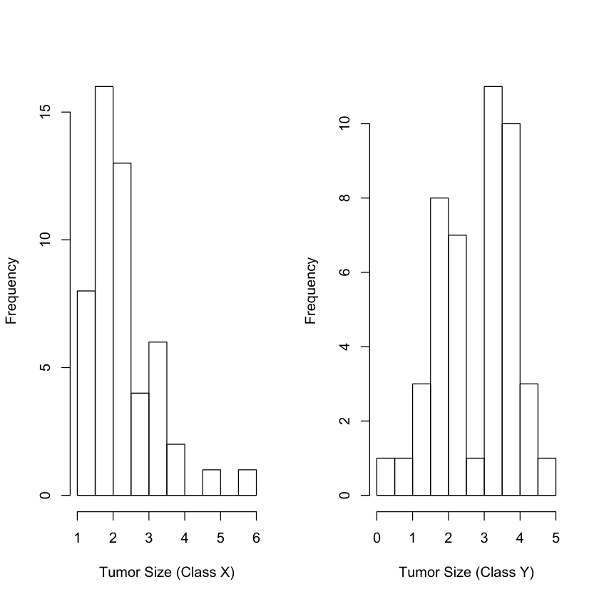
Breast cancer is the second leading cause of deaths from cancer among women in the United States. Despite major progresses in breast cancer treatment, the ability to predict the metastatic behavior of tumor remains limited. This breast cancer study was first reported in van’t Veer et al. (2002) where 97 lymph node-negative breast cancer patients, 55 years old or younger, participated in this study. Among them, 46 developed distant metastases within 5 years (XX class) and 51 remained metastases free for at least 5 years (YY class). In this study, covariates including clinical risk factors (tumor size, age, histological grade etc.) as well as expression levels for 24,481 gene probes were collected. The histograms of the tumor sizes for both classes are presented in Figure 3. Shapiro’s normality test is used to test the normality of the tumor size with pp-value <0.001<0.001 for class XX and 0.2210.221 for class YY, indicating that it might not be suitable to treat tumor size as one of the covariates to conduct classification using the LPD rule. On the other hand, as introduced before, Figure 1 indicates that the gene expression levels for patients in the XX class and the YY class vary differently as tumor size changes. We thus set the tumor size as the dynamic factor. For comparison, we also consider the LPD rule with or without including the tumor size as one of the covariates, denoted as “LPD with UU” and “LPD without UU”, respectively. The intercept is chosen according to Proposition 2 of Mai, Zou & Yuan (2012). For simplicity, we use the pp genes with the largest absolute tt-statistic values between the two groups for discriminant analysis, and in our study we set p=25,50,100p=25,50,100 and 200200. We randomly choose 92 observations as training samples and set the rest 5 observations as test samples. This procedure is repeated for 100 times. The mean misclassification rate and its standard deviation over 100 replications are reported in Table 2. From the results we can see that no significant improvement is observed when the tumor size is included as one of the covariate in the LPD rule. However, when it is set to be a dynamic factor as in our DLPD rule, the misclassification rate of is seen to be reduced.
Refer to caption
Figure 3: Histogram of tumor sizes in the XX and YY classes of the Breast Cancer data.
p LPD without UU LPD with UU DLPD
25 0.198 (0.018) 0.198 (0.018) 0.190 (0.018)
50 0.184 (0.016) 0.184 (0.016) 0.170 (0.016)
100 0.186 (0.015) 0.184 (0.016) 0.172 (0.015)
200 0.216 (0.019) 0.216 (0.020) 0.204 (0.019)
Table 2: Mean classification rate and its standard deviation for the Breast Cancer study over 100 replications.

5 Conclusion and discussion

We have proposed a new and simple model for high dimensional linear discriminant analysis when data is high-dimensional and the local features of the data can play important roles in classification. Our approach combines the simplicity of kernel smoothing and the powerful method of regularization for studying high dimensional problems. We have established uniform Bernstein-type inequalities for our high-dimensional nonparametric estimators, and shown that the risk function of the proposed DLPD rule converges to the optimal Bayes risk in probability under general sparsity assumptions, uniformly over the range of the covariates. The minimax lower bounds for the estimation of the Bayes risk are also established, and it is shown that the misclassification rate of our proposed rule is minimax-rate optimal. Both the uniform convergence and the minimax results appear to be new in the literature of classification.

A limitation of the linear discriminant rule is its Gaussian assumption. An immediate generalization of our method is to allow a more flexible family of distributions, for example, the transnormal family in Lin & Jeon (2003). On the other hand, the smoothness assumption (A6) might not be appropriate in some cases. For example, discontinuity of the brain activity is common in certain applications (Vairavan et al., 2009), leading to discontinuous μ⁡(𝐮)\mu({\bf u}) and Σ⁡(𝐮)\Sigma({\bf u}) which are usually modeled as piecewise-continuous functions. This gives rise to a similar problem as ours where the aim is to identify the number of the discontinuous points and their locations. We also remark that the assumption of independent observations (Xi,𝐔i),i=1,…,n1,(Yj,𝐕j),j=1,…,n2(X_{i},{\bf U}_{i}),i=1,\ldots,n_{1},(Y_{j},{\bf V}_{j}),j=1,\ldots,n_{2} can be relaxed to that Xi|𝐔i,i=1,…,n1,Yj|𝐕j,j=1,…,n2X_{i}|{\bf U}_{i},i=1,\ldots,n_{1},Y_{j}|{\bf V}_{j},j=1,\ldots,n_{2} are weakly dependent, which might enable us to incorporate temporal correlations. Under suitable weakly dependence assumptions such as strongly mixing (Merlevede, Peligrad & Rios, 2009), estimators of the components in the Bayes rule proposed in Section 2 can be shown consistent. Nevertheless, for time series data, it would be interesting to incorporate our DLPD rule with time series models so as to capture the structures of the covariance matrix and the dependency among the sequences of observations. This is beyond the scope of the current paper and will be studied elsewhere.

In our work, we have assumed that ΣX​(𝐮)=ΣY​(𝐮)\Sigma_{X}({\bf u})=\Sigma_{Y}({\bf u}) which seems to be reasonable for the data analysis. It is however worth considering problems where covariances are dynamic but not equal. Finally, we have only discussed binary classification in this paper. It will be interesting to extend this work to study multiclass classification (Pan, Wang & Li, 2015; Mai, Yang & Zou, 2015), and other recent approaches which considered more complex structures (Niu, Hao & Dong, 2015). Last but not least, in the unbalanced case, the cut-off point in the Bayes procedure becomes log⁡(π2/π1)\log(\pi_{2}/\pi_{1}), which is usually estimated by log⁡(n2/n1)\log(n_{2}/n_{1}). Here π1\pi_{1} is the prior probability of observing a sample from Class XX and π2=1−π1\pi_{2}=1-\pi_{1}. However, as pointed out in Mai, Zou & Yuan (2012), the problem of finding the right cut-off point receives little attention in the literature and it is also important to find a optimal estimator of the cut-off points to improve classification accuracy.

One alternative of our DLPD rule is to develop a dynamic logistic regression model in which a rule is obtained by minimizing a dynamic version of the penalized entropy loss. It is well know that under Gaussian assumptions, logistic regression and LDA are equivalent in that the solution (in a population sense) of logistic regression is exactly the Bayes rule. For the fixed dimension and static case, earlier numerical studies have shown that logistic regression and LDA would give the same linear discriminant function (Press and Wilson, 1978), while theoretically, Efron (1975) showed that LDA is more efficient than logistic regression under the Gaussian assumptions. On one hand, it is worth exploring the theoretical properties of logistic regression based rules under the more general sparsity assumption (3.1). On the other hand, it would be interesting and challenging to compare the efficiency of logistic regression rules and LDA rules under both high dimensional and non-stationary assumptions.

As pointed out in Candes & Tao (2007), a two-stage procedure generally produces better estimation results in the strict sparse case where many parameters are zero. When the true discriminant direction β⁡(u)\beta(u) is sparse, we may use a two-stage procedure similar to the one in Jiang & Leng (2016). That is, in the first stage, the same bandwidth is used to obtain a sparse first stage estimator β^​(u)\hat{\beta}(u). In the second stage, we can apply our approach again to estimate the identified nonzero elements in β^​(u)\hat{\beta}(u). If the number of nonzeros in the second stage is very low, different bandwidths can be considered for different elements.

Appendix A

Before we proceed to the proofs for the main theorems, we introduce some technical lemmas.

Lemma 3.

Suppose ϵn→0\epsilon_{n}\rightarrow 0, n​|Hx|​ϵn2→∞n|H_{x}|\epsilon_{n}^{2}\rightarrow\infty and there exists a large enough constant ChC_{h} such that ϵn2>Ch​(hx4+hy4)\epsilon^{2}_{n}>C_{h}(h_{x}^{4}+h_{y}^{4}). Under assumptions (A1)-(A6), there exist constants C1>0C_{1}>0 and C2>0C_{2}>0 such that

P⁡(sup𝐮∈Ωd|1n1​∑i=1n1𝐊Hx​(𝐔i−𝐮)−f⁡(𝐮)|≥ϵn)\displaystyle P\Big(\sup_{{\bf u}\in\Omega_{d}}\Big|\frac{1}{n_{1}}\sum_{i=1}^{n_{1}}{\bf K}_{H_{x}}({\bf U}_{i}-{\bf u})-f({\bf u})\Big|\geq\epsilon_{n}\Big)
≤\displaystyle\leq C1​(nlog⁡p)44+d​exp⁡{−C2​n​(log⁡pn)d4+d​ϵn2};\displaystyle C_{1}\left(\frac{n}{\log p}\right)^{\frac{4}{4+d}}\exp\left\{-C_{2}n\left(\frac{\log p}{n}\right)^{\frac{d}{4+d}}\epsilon_{n}^{2}\right\};

and

P⁡(sup𝐮∈Ωd|1n2​∑i=1n2𝐊Hy​(𝐕i−𝐮)−f⁡(𝐮)|≥ϵn)\displaystyle P\Big(\sup_{{\bf u}\in\Omega_{d}}\Big|\frac{1}{n_{2}}\sum_{i=1}^{n_{2}}{\bf K}_{H_{y}}({\bf V}_{i}-{\bf u})-f({\bf u})\Big|\geq\epsilon_{n}\Big)
≤\displaystyle\leq C1​(nlog⁡p)44+d​exp⁡{−C2​n​(log⁡pn)d4+d​ϵn2}.\displaystyle C_{1}\left(\frac{n}{\log p}\right)^{\frac{4}{4+d}}\exp\left\{-C_{2}n\left(\frac{\log p}{n}\right)^{\frac{d}{4+d}}\epsilon_{n}^{2}\right\}.
Proof.

Without loss of generality, assume that Ωd=[a1,b1]×⋯[ad,bd]\Omega_{d}=[a_{1},b_{1}]\times\cdots[a_{d},b_{d}] and decompose it as Ωd=∪1≤ij≤qj,j=1,…,dωi1,…,id\Omega_{d}=\cup_{1\leq i_{j}\leq q_{j},j=1,\ldots,d}\omega_{i_{1},\ldots,i_{d}}, where qj=bj−aj2​hx​j4q_{j}=\frac{b_{j}-a_{j}}{2h_{xj}^{4}} for j=1,…,dj=1,\ldots,d and ωi1,…,id=[a1+2(i1−1)hx​14,a1+2i1hx​14]×⋯×[ad+2(id−1)hx​d4,ad+2idhx​d4]\omega_{i_{1},\ldots,i_{d}}=[a_{1}+2(i_{1}-1)h_{x1}^{4},a_{1}+2i_{1}h_{x1}^{4}]\times\cdots\times[a_{d}+2(i_{d}-1)h_{xd}^{4},a_{d}+2i_{d}h_{xd}^{4}]. Denote Wi​(𝐮)=[𝐊Hx​(𝐔i−𝐮)−E​𝐊Hx​(𝐔i−𝐮)]/n1W_{i}({\bf u})=[{\bf K}_{H_{x}}({\bf U}_{i}-{\bf u})-E{\bf K}_{H_{x}}({\bf U}_{i}-{\bf u})]/n_{1}. We then have: for any 𝐮∈Ωd{\bf u}\in\Omega_{d}, using assumption (A1) and Markov’s inequality we have, for any 0<t<n1​|Hx|2​K10<t<\frac{n_{1}|H_{x}|}{2K_{1}},

P⁡(|1n1​∑j=1n1𝐊Hx​(𝐔j−𝐮)−E​𝐊Hx​(𝐔i−𝐮)|>ϵn)\displaystyle P\left(\Big|\frac{1}{n_{1}}\sum_{j=1}^{n_{1}}{\bf K}_{H_{x}}({\bf U}_{j}-{\bf u})-E{\bf K}_{H_{x}}({\bf U}_{i}-{\bf u})\Big|>\epsilon_{n}\right) (15)
≤\displaystyle\leq 2​exp⁡{−t​ϵn}​Πi=1n1​E​exp​{t​Wi​(𝐮)}\displaystyle 2\exp\{-t\epsilon_{n}\}\Pi_{i=1}^{n_{1}}E\exp\{tW_{i}({\bf u})\}
≤\displaystyle\leq 2​exp⁡{−t​ϵn}​Πi=1n1​{1+t2​E​Wi​(𝐮)2}\displaystyle 2\exp\{-t\epsilon_{n}\}\Pi_{i=1}^{n_{1}}\{1+t^{2}EW_{i}({\bf u})^{2}\}
≤\displaystyle\leq 2​exp⁡{−t​ϵn+∑i=1n1t2​E​Wi​(𝐮)2}\displaystyle 2\exp\left\{-t\epsilon_{n}+\sum_{i=1}^{n_{1}}t^{2}EW_{i}({\bf u})^{2}\right\}
≤\displaystyle\leq 2​exp⁡{−t​ϵn+C​t2n1​|Hx|},\displaystyle 2\exp\left\{-t\epsilon_{n}+\frac{Ct^{2}}{n_{1}|H_{x}|}\right\},

for some large enough constant CC. By setting t=(2​C)−1​n1​|Hx|​ϵnt=(2C)^{-1}n_{1}|H_{x}|\epsilon_{n}, we have:

P⁡(|1n1​∑j=1n1𝐊Hx​(𝐔j−𝐮)−E​𝐊Hx​(𝐔i−𝐮)|>ϵn)≤2​exp⁡{−ϵn2​n1​|Hx|4​C}.P\left(\Big|\frac{1}{n_{1}}\sum_{j=1}^{n_{1}}{\bf K}_{H_{x}}({\bf U}_{j}-{\bf u})-E{\bf K}_{H_{x}}({\bf U}_{i}-{\bf u})\Big|>\epsilon_{n}\right)\leq 2\exp\left\{-\frac{\epsilon_{n}^{2}n_{1}|H_{x}|}{4C}\right\}. (16)

Write 𝐮i1,…,id=(a1+2​i1​hx​14,⋯,ad+2​id​hx​d4)T{\bf u}_{i_{1},\ldots,i_{d}}=(a_{1}+2i_{1}h_{x1}^{4},\cdots,a_{d}+2i_{d}h_{xd}^{4})^{T} for 1≤ij≤qj,j=1,…,d1\leq i_{j}\leq q_{j},j=1,\ldots,d. Note that

sup𝐮∈Ωd|1n1​∑j=1n1𝐊Hx​(𝐔j−𝐮)−E​𝐊Hx​(𝐔i−𝐮)|\displaystyle\sup_{{\bf u}\in\Omega_{d}}\Big|\frac{1}{n_{1}}\sum_{j=1}^{n_{1}}{\bf K}_{H_{x}}({\bf U}_{j}-{\bf u})-E{\bf K}_{H_{x}}({\bf U}_{i}-{\bf u})\Big| (17)
≤\displaystyle\leq max1≤ij≤qj,j=1,…,d|1n1∑j=1n1𝐊Hx(𝐔j−𝐮i1,…,id)−E𝐊Hx(𝐔i−𝐮i1,…,id)|+\displaystyle\max_{1\leq i_{j}\leq q_{j},j=1,\ldots,d}\Big|\frac{1}{n_{1}}\sum_{j=1}^{n_{1}}{\bf K}_{H_{x}}({\bf U}_{j}-{\bf u}_{i_{1},\ldots,i_{d}})-E{\bf K}_{H_{x}}({\bf U}_{i}-{\bf u}_{i_{1},\ldots,i_{d}})\Big|+
max1≤ij≤qj,j=1,…,dsup𝐮∈ωi1,…,id|1n1∑j=1n1𝐊Hx(𝐔j−𝐮)−1n1∑j=1n1𝐊Hx(𝐔j−𝐮i1,…,id)\displaystyle\max_{1\leq i_{j}\leq q_{j},j=1,\ldots,d}\sup_{{\bf u}\in\omega_{i_{1},\ldots,i_{d}}}\Big|\frac{1}{n_{1}}\sum_{j=1}^{n_{1}}{\bf K}_{H_{x}}({\bf U}_{j}-{\bf u})-\frac{1}{n_{1}}\sum_{j=1}^{n_{1}}{\bf K}_{H_{x}}({\bf U}_{j}-{\bf u}_{i_{1},\ldots,i_{d}})
−[E𝐊Hx(𝐔i−𝐮)−E𝐊Hx(𝐔i−𝐮i1,…,id)]|.\displaystyle-[E{\bf K}_{H_{x}}({\bf U}_{i}-{\bf u})-E{\bf K}_{H_{x}}({\bf U}_{i}-{\bf u}_{i_{1},\ldots,i_{d}})]\Big|.

Denote diag⁡(Hx4)=(hx​14,…,hx​d4)T{\rm diag}(H^{4}_{x})=(h^{4}_{x1},\ldots,h_{xd}^{4})^{T}. For each (i1,…,id)(i_{1},\ldots,i_{d}), using the mean value theorem and assumption (A1) we have, there exist random scalars 0≤Ri1,…,id≤20\leq R_{i_{1},\ldots,i_{d}}\leq 2 depending on 𝐔1,…,𝐔n1{\bf U}_{1},\ldots,{\bf U}_{n_{1}} such that

sup𝐮∈ωi1,…,id|1n1​∑j=1n1𝐊Hx​(𝐔j−𝐮)−1n1​∑j=1n1𝐊Hx​(𝐔j−𝐮i1,…,id)|\displaystyle\sup_{{\bf u}\in\omega_{i_{1},\ldots,i_{d}}}\Big|\frac{1}{n_{1}}\sum_{j=1}^{n_{1}}{\bf K}_{H_{x}}({\bf U}_{j}-{\bf u})-\frac{1}{n_{1}}\sum_{j=1}^{n_{1}}{\bf K}_{H_{x}}({\bf U}_{j}-{\bf u}_{i_{1},\ldots,i_{d}})\Big| (18)
≤\displaystyle\leq 2​tr​(Hx3)n1​∑j=1n1supu∈ωi1,…,id|𝐊Hx′​(𝐔j−𝐮i1,…,id+Ri1,…,id​diag​(Hx4))|∞\displaystyle\frac{2{\rm tr}(H^{3}_{x})}{n_{1}}\sum_{j=1}^{n_{1}}\sup_{u\in\omega_{i_{1},\ldots,i_{d}}}\Big|{\bf K}^{\prime}_{H_{x}}({\bf U}_{j}-{\bf u}_{i_{1},\ldots,i_{d}}+R_{i_{1},\ldots,i_{d}}{\rm diag}(H_{x}^{4}))\Big|_{\infty}
≤\displaystyle\leq 2​K2​tr​(Hx3).\displaystyle 2K_{2}{\rm tr}(H^{3}_{x}).

On the other hand, it can be easily shown that

max1≤ij≤qj,j=1,…,dsup𝐮∈ωi1,…,id[E𝐊Hx(𝐔i−𝐮)−E𝐊Hx(𝐔i−𝐮i1,…,id)]=O(tr(Hx4)).\max_{1\leq i_{j}\leq q_{j},j=1,\ldots,d}\sup_{{\bf u}\in\omega_{i_{1},\ldots,i_{d}}}[E{\bf K}_{H_{x}}({\bf U}_{i}-{\bf u})-E{\bf K}_{H_{x}}({\bf U}_{i}-{\bf u}_{i_{1},\ldots,i_{d}})]=\emph{O}({\rm tr}(H^{4}_{x})). (19)

Combining (16), (17), (18) and (19) with the assumption on ϵn\epsilon_{n}, we have

P⁡(sup𝐮∈Ωd|1n1​∑j=1n1𝐊Hx​(𝐔j−𝐮)−E​𝐊Hx​(𝐔i−𝐮)|>ϵn)\displaystyle P\left(\sup_{{\bf u}\in\Omega_{d}}\Big|\frac{1}{n_{1}}\sum_{j=1}^{n_{1}}{\bf K}_{H_{x}}({\bf U}_{j}-{\bf u})-E{\bf K}_{H_{x}}({\bf U}_{i}-{\bf u})\Big|>\epsilon_{n}\right) (20)
≤c1q1⋯qdexp{−c2n1|Hx|ϵn2}\displaystyle\leq c_{1}q_{1}\cdots q_{d}\exp\{-c_{2}n_{1}|H_{x}|\epsilon_{n}^{2}\}
=C1​(n1log⁡p)4/(4+d)​exp⁡{−C2​n1​hxd​ϵn2},\displaystyle=C_{1}\left(\frac{n_{1}}{\log p}\right)^{4/(4+d)}\exp\{-C_{2}n_{1}h_{x}^{d}\epsilon_{n}^{2}\},

for some constants c1>0,c2>0,C1>0,C2>0c_{1}>0,c_{2}>0,C_{1}>0,C_{2}>0. The first argument of Lemma 3 is then proved by combining (20) and the following well known result (see for example Pagan & Ullah (1999)):

supu∈Ωd|E​𝐊Hx​(𝐔i−𝐮)−f⁡(𝐮)|=​O​(tr​H2).\displaystyle\sup_{u\in\Omega_{d}}|E{\bf K}_{H_{x}}({\bf U}_{i}-{\bf u})-f({\bf u})|=\emph{O}({\rm tr}H^{2}).

The second argument of Lemma 3 can be proved similarly.

∎

Lemma 4 and Lemma 5 below give the Bernstein-type inequalities (uniformly in 𝐮∈Ωd{\bf u}\in\Omega_{d}) for the functional estimators of the means and covariance matrix defined as in (3), (4) and (5). We only provide the proof for Lemma 5 and the proof for Lemma 4 is similar.

Lemma 4.

Suppose ϵn→0\epsilon_{n}\rightarrow 0, n​|Hx|​ϵn2→∞n|H_{x}|\epsilon_{n}^{2}\rightarrow\infty and there exists a large enough constant ChC_{h} such that ϵn2>Ch​(hx4+hy4)\epsilon^{2}_{n}>C_{h}(h_{x}^{4}+h_{y}^{4}). Under assumptions (A1)-(A6), there exist constants C3>0C_{3}>0 and C4>0C_{4}>0 such that

P⁡(max⁡sup𝐮∈Ωd1≤i≤p⁡|μ^Xi​(𝐮)−μXi​(𝐮)|≥ϵn)\displaystyle P\bigg(\max_{1\leq i\leq p}\sup_{{\bf u}\in\Omega_{d}}|\hat{\mu}_{X}^{i}({\bf u})-\mu_{X}^{i}({\bf u})|\geq\epsilon_{n}\bigg)
≤\displaystyle\leq C3​p​(nlog⁡p)44+d​exp⁡{−C4​n​(log⁡pn)d4+d​ϵn2},\displaystyle C_{3}p\left(\frac{n}{\log p}\right)^{\frac{4}{4+d}}\exp\left\{-C_{4}n\left(\frac{\log p}{n}\right)^{\frac{d}{4+d}}\epsilon_{n}^{2}\right\},

and

P⁡(max⁡sup𝐮∈Ωd1≤i≤p⁡|μ^Yi​(𝐮)−μYi​(𝐮)|≥ϵn)\displaystyle P\bigg(\max_{1\leq i\leq p}\sup_{{\bf u}\in\Omega_{d}}|\hat{\mu}_{Y}^{i}({\bf u})-\mu_{Y}^{i}({\bf u})|\geq\epsilon_{n}\bigg)
≤\displaystyle\leq C3​p​(nlog⁡p)44+d​exp⁡{−C4​n​(log⁡pn)d4+d​ϵn2}.\displaystyle C_{3}p\left(\frac{n}{\log p}\right)^{\frac{4}{4+d}}\exp\left\{-C_{4}n\left(\frac{\log p}{n}\right)^{\frac{d}{4+d}}\epsilon_{n}^{2}\right\}.
Lemma 5.

Suppose ϵn→0\epsilon_{n}\rightarrow 0, n​|Hx|​ϵn2→∞n|H_{x}|\epsilon_{n}^{2}\rightarrow\infty and there exists a large enough constant ChC_{h} such that ϵn2>Ch​(hx4+hy4)\epsilon^{2}_{n}>C_{h}(h_{x}^{4}+h_{y}^{4}). Under assumptions (A1)-(A6), there exist constants C5>0C_{5}>0 and C6>0C_{6}>0 such that

P⁡(max⁡sup𝐮∈Ωd1≤i,j≤p⁡|σ^i​j​(𝐮)−σi​j​(𝐮)|≥ϵn)\displaystyle P\bigg(\max_{1\leq i,j\leq p}\sup_{{\bf u}\in\Omega_{d}}|\hat{\sigma}_{ij}({\bf u})-\sigma_{ij}({\bf u})|\geq\epsilon_{n}\bigg)
≤\displaystyle\leq C5​p2​(nlog⁡p)44+d​exp⁡{−C6​n​(log⁡pn)d4+d​ϵn2}.\displaystyle C_{5}p^{2}\left(\frac{n}{\log p}\right)^{\frac{4}{4+d}}\exp\left\{-C_{6}n\left(\frac{\log p}{n}\right)^{\frac{d}{4+d}}\epsilon_{n}^{2}\right\}.
Proof.

We first show that there exist positive constants c1,c2c_{1},c_{2} such that

P⁡(max⁡sup𝐮∈Ωd1≤i,j≤p⁡|1n1​∑k=1n1𝐊Hx​(𝐔k−𝐮)​Xk​i​Xk​j−E⁡(X1​i​X1​j|𝐔1=𝐮)​f​(𝐮)|≥ϵn)\displaystyle P\bigg(\max_{1\leq i,j\leq p}\sup_{{\bf u}\in\Omega_{d}}\Big|\frac{1}{n_{1}}\sum_{k=1}^{n_{1}}{\bf K}_{H_{x}}({\bf U}_{k}-{\bf u})X_{ki}X_{kj}-E(X_{1i}X_{1j}|{\bf U}_{1}={\bf u})f({\bf u})\Big|\geq\epsilon_{n}\bigg) (21)
≤c1​p2​(nlog⁡p)44+d​exp⁡{−c2​n​(log⁡pn)d4+d​ϵn2}.\displaystyle\leq c_{1}p^{2}\left(\frac{n}{\log p}\right)^{\frac{4}{4+d}}\exp\left\{-c_{2}n\left(\frac{\log p}{n}\right)^{\frac{d}{4+d}}\epsilon_{n}^{2}\right\}.

Denote Wk​i​j​(𝐮)=[𝐊Hx​(𝐔k−𝐮)​Xk​i​Xk​j−E​𝐊Hx​(𝐔k−𝐮)​Xk​i​Xk​j]/n1W_{kij}({\bf u})=[{\bf K}_{H_{x}}({\bf U}_{k}-{\bf u})X_{ki}X_{kj}-E{\bf K}_{H_{x}}({\bf U}_{k}-{\bf u})X_{ki}X_{kj}]/n_{1} and M=max1≤l≤p⁡E​X1​l4M=\max_{1\leq l\leq p}EX_{1l}^{4}. Notice that

E​Wk​i​j​(𝐮)2≤4​K12​dn12​|Hx2|​E​Xk​i2​Xk​j2≤2​K12​dn12​|Hx2|​E​(Xk​i4+Xk​j4)≤4​K12​d​Mn12​|Hx2|.\displaystyle EW_{kij}({\bf u})^{2}\leq\frac{4{K}_{1}^{2d}}{n_{1}^{2}|H_{x}^{2}|}EX_{ki}^{2}X_{kj}^{2}\leq\frac{2K_{1}^{2d}}{n_{1}^{2}|H_{x}^{2}|}E(X_{ki}^{4}+X_{kj}^{4})\leq\frac{4K_{1}^{2d}M}{n_{1}^{2}|H_{x}^{2}|}.

For any 𝐮∈Ωd{\bf u}\in\Omega_{d}, using Markov’s inequality we have, for any 0<t<n1​|Hx|2​K1d​M1/20<t<\frac{n_{1}|H_{x}|}{2K_{1}^{d}M^{1/2}},

P⁡(|1n1​∑k=1n1𝐊Hx​(𝐔k−𝐮)​Xk​i​Xk​j−E​𝐊Hx​(𝐔k−𝐮)​Xk​i​Xk​j|>ϵn)\displaystyle P\left(\Big|\frac{1}{n_{1}}\sum_{k=1}^{n_{1}}{\bf K}_{H_{x}}({\bf U}_{k}-{\bf u})X_{ki}X_{kj}-E{\bf K}_{H_{x}}({\bf U}_{k}-{\bf u})X_{ki}X_{kj}\Big|>\epsilon_{n}\right) (22)
≤\displaystyle\leq 2​exp⁡{−t​ϵn}​Πk=1n1​E​exp​{t​Wk​i​j​(𝐮)}\displaystyle 2\exp\{-t\epsilon_{n}\}\Pi_{k=1}^{n_{1}}E\exp\{tW_{kij}({\bf u})\}
≤\displaystyle\leq 2​exp⁡{−t​ϵn}​Πk=1n1​{1+t2​E​Wk​i​j​(𝐮)2}\displaystyle 2\exp\{-t\epsilon_{n}\}\Pi_{k=1}^{n_{1}}\{1+t^{2}EW_{kij}({\bf u})^{2}\}
≤\displaystyle\leq 2​exp⁡{−t​ϵn+∑k=1n1t2​E​Wk​i​j​(𝐮)2}\displaystyle 2\exp\left\{-t\epsilon_{n}+\sum_{k=1}^{n_{1}}t^{2}EW_{kij}({\bf u})^{2}\right\}
≤\displaystyle\leq 2​exp⁡{−t​ϵn+C​t2n1​|Hx|},\displaystyle 2\exp\left\{-t\epsilon_{n}+\frac{Ct^{2}}{n_{1}|H_{x}|}\right\},

for some large enough constant CC. Here in the last step we have used the fact that V​a​r​(Wk​i​j​(𝐮))=​O​(n1−2​|Hx|−1)Var(W_{kij}({\bf u}))=\emph{O}(n_{1}^{-2}|H_{x}|^{-1}). By setting t=(2​C)−1​n1​|Hx|​ϵnt=(2C)^{-1}n_{1}|H_{x}|\epsilon_{n}, we have:

P⁡(|1n1​∑k=1n1𝐊Hx​(𝐔k−𝐮)​Xk​i​Xk​j−E​𝐊Hx​(𝐔k−𝐮)​Xk​i​Xk​j|>ϵn)\displaystyle P\left(\Big|\frac{1}{n_{1}}\sum_{k=1}^{n_{1}}{\bf K}_{H_{x}}({\bf U}_{k}-{\bf u})X_{ki}X_{kj}-E{\bf K}_{H_{x}}({\bf U}_{k}-{\bf u})X_{ki}X_{kj}\Big|>\epsilon_{n}\right) (23)
≤\displaystyle\leq 2​exp⁡{−ϵn2​n1​|Hx|4​C}.\displaystyle 2\exp\left\{-\frac{\epsilon_{n}^{2}n_{1}|H_{x}|}{4C}\right\}.

Again, without loss of generality, assume that Ωd=[a1,b1]×⋯[ad,bd]\Omega_{d}=[a_{1},b_{1}]\times\cdots[a_{d},b_{d}] and let q1,…,qdq_{1},\ldots,q_{d}, ωi1,…,id\omega_{i_{1},\ldots,i_{d}} and 𝐮i1,…,id{\bf u}_{i_{1},\ldots,i_{d}} for 1≤ij≤qj,1≤j≤d1\leq i_{j}\leq q_{j},1\leq j\leq d be defined as in the proof of Lemma 3.

Note that

sup𝐮∈Ωd|1n1​∑k=1n1𝐊Hx​(𝐔j−𝐮)​Xk​i​Xk​j−E​𝐊Hx​(𝐔j−𝐮)​Xk​i​Xk​j|\displaystyle\sup_{{\bf u}\in\Omega_{d}}\Big|\frac{1}{n_{1}}\sum_{k=1}^{n_{1}}{\bf K}_{H_{x}}({\bf U}_{j}-{\bf u})X_{ki}X_{kj}-E{\bf K}_{H_{x}}({\bf U}_{j}-{\bf u})X_{ki}X_{kj}\Big| (24)
≤\displaystyle\leq max1≤ij≤qj,j=1,…,d|1n1∑k=1n1𝐊Hx(𝐔j−𝐮i1,…,id)Xk​iXk​j\displaystyle\max_{1\leq i_{j}\leq q_{j},j=1,\ldots,d}\Big|\frac{1}{n_{1}}\sum_{k=1}^{n_{1}}{\bf K}_{H_{x}}({\bf U}_{j}-{\bf u}_{i_{1},\ldots,i_{d}})X_{ki}X_{kj}
−E𝐊Hx(𝐔j−𝐮i1,…,id)Xk​iXk​j|\displaystyle-E{\bf K}_{H_{x}}({\bf U}_{j}-{\bf u}_{i_{1},\ldots,i_{d}})X_{ki}X_{kj}\Big|
+max1≤ij≤qj,j=1,…,dsup𝐮∈ωi1,…,id|1n1∑k=1n1𝐊Hx(𝐔j−𝐮)Xk​iXk​j\displaystyle+\max_{1\leq i_{j}\leq q_{j},j=1,\ldots,d}\sup_{{\bf u}\in\omega_{i_{1},\ldots,i_{d}}}\Big|\frac{1}{n_{1}}\sum_{k=1}^{n_{1}}{\bf K}_{H_{x}}({\bf U}_{j}-{\bf u})X_{ki}X_{kj}
−1n1∑k=1n1𝐊Hx(𝐔j−𝐮i1,…,id)Xk​iXk​j\displaystyle-\frac{1}{n_{1}}\sum_{k=1}^{n_{1}}{\bf K}_{H_{x}}({\bf U}_{j}-{\bf u}_{i_{1},\ldots,i_{d}})X_{ki}X_{kj}
−[E𝐊Hx(𝐔i−𝐮)Xk​iXk​j−E𝐊Hx(𝐔i−𝐮i1,…,id)Xk​iXk​j]|.\displaystyle-[E{\bf K}_{H_{x}}({\bf U}_{i}-{\bf u})X_{ki}X_{kj}-E{\bf K}_{H_{x}}({\bf U}_{i}-{\bf u}_{i_{1},\ldots,i_{d}})X_{ki}X_{kj}]\Big|.

Using the mean value theorem we have, there exists a random scalars 0≤Ri1,…,id≤20\leq R_{i_{1},\ldots,i_{d}}\leq 2 depending on 𝐔1,…,𝐔n1{\bf U}_{1},\ldots,{\bf U}_{n_{1}} such that

sup𝐮∈ωi1,…,id|1n1​∑k=1n1𝐊Hx​(𝐔j−𝐮)​Xk​i​Xk​j−1n1​∑k=1n1𝐊Hx​(𝐔j−𝐮i1,…,id)​Xk​i​Xk​j|\displaystyle\sup_{{\bf u}\in\omega_{i_{1},\ldots,i_{d}}}\Big|\frac{1}{n_{1}}\sum_{k=1}^{n_{1}}{\bf K}_{H_{x}}({\bf U}_{j}-{\bf u})X_{ki}X_{kj}-\frac{1}{n_{1}}\sum_{k=1}^{n_{1}}{\bf K}_{H_{x}}({\bf U}_{j}-{\bf u}_{i_{1},\ldots,i_{d}})X_{ki}X_{kj}\Big|
≤2​tr​(Hx3)n1​supu∈ωi1,…,id|∑k=1n1𝐊Hx′​(𝐔j−𝐮i1,…,id+Ri1,…,id​diag​(Hx4))​Xk​i​Xk​j|\displaystyle\leq\frac{2{\rm tr}(H^{3}_{x})}{n_{1}}\sup_{u\in\omega_{i_{1},\ldots,i_{d}}}\Big|\sum_{k=1}^{n_{1}}{\bf K}^{\prime}_{H_{x}}({\bf U}_{j}-{\bf u}_{i_{1},\ldots,i_{d}}+R_{i_{1},\ldots,i_{d}}{\rm diag}(H_{x}^{4}))X_{ki}X_{kj}\Big|
≤K2​tr​(Hx3)n1​∑k=1n1(Xk​i2+Xk​j2).\displaystyle\leq\frac{K_{2}{\rm tr}(H^{3}_{x})}{n_{1}}\sum_{k=1}^{n_{1}}(X_{ki}^{2}+X_{kj}^{2}).

Note that assumption (A5) implies that there exists a constant M1<∞M_{1}<\infty such that for any 1≤i≤p1\leq i\leq p,

sup𝐮∈Ωd|μXi​(𝐮)|≤M1,sup𝐮∈Ωd|μYi​(𝐮)|≤M1,sup𝐮∈Ωd|σi​i​(𝐮)|≤M1.\sup_{{\bf u}\in\Omega_{d}}|\mu_{X}^{i}({\bf u})|\leq M_{1},~~~\sup_{{\bf u}\in\Omega_{d}}|\mu_{Y}^{i}({\bf u})|\leq M_{1},~~~\sup_{{\bf u}\in\Omega_{d}}|\sigma_{ii}({\bf u})|\leq M_{1}.

By verifying the conditions of Bernstein’s inequality (see for example Lin & Bai (2010)), we have that

P⁡(1n1​∑k=1n1Xk​i2>M12+M1+1)=b1​exp⁡{−b2​n1},\displaystyle P\left(\frac{1}{n_{1}}\sum_{k=1}^{n_{1}}X_{ki}^{2}>M_{1}^{2}+M_{1}+1\right)=b_{1}\exp\{-b_{2}n_{1}\},

for some positive constants b1,b2b_{1},b_{2}. Therefore, with probability greater than 1−b1​exp⁡{−b2​n1}1-b_{1}\exp\{-b_{2}n_{1}\},

sup𝐮∈ωi1,…,id|1n1​∑k=1n1𝐊Hx​(𝐔j−𝐮)​Xk​i​Xk​j−1n1​∑k=1n1𝐊Hx​(𝐔j−𝐮i1,…,id)​Xk​i​Xk​j|\displaystyle\sup_{{\bf u}\in\omega_{i_{1},\ldots,i_{d}}}\Big|\frac{1}{n_{1}}\sum_{k=1}^{n_{1}}{\bf K}_{H_{x}}({\bf U}_{j}-{\bf u})X_{ki}X_{kj}-\frac{1}{n_{1}}\sum_{k=1}^{n_{1}}{\bf K}_{H_{x}}({\bf U}_{j}-{\bf u}_{i_{1},\ldots,i_{d}})X_{ki}X_{kj}\Big| (25)
≤K2​tr​(Hx3)​(M12+M1+1)n1.\displaystyle\leq\frac{K_{2}{\rm tr}(H^{3}_{x})(M_{1}^{2}+M_{1}+1)}{n_{1}}.

Clearly, b1​exp⁡{−b2​n1}b_{1}\exp\{-b_{2}n_{1}\} is negligible comparing to the right hand side of (21). On the other hand, by conditional on 𝐔k{\bf U}_{k} first, we obtain:

max1≤ij≤qj,j=1,…,dsup𝐮∈ωi1,…,id\displaystyle\max_{1\leq i_{j}\leq q_{j},j=1,\ldots,d}\sup_{{\bf u}\in\omega_{i_{1},\ldots,i_{d}}} [E𝐊Hx(𝐔k−𝐮)Xk​iXk​j\displaystyle[E{\bf K}_{H_{x}}({\bf U}_{k}-{\bf u})X_{ki}X_{kj} (26)
−E𝐊Hx(𝐔i−𝐮i1,…,id)Xk​iXk​j]=O(tr(Hx4)).\displaystyle-E{\bf K}_{H_{x}}({\bf U}_{i}-{\bf u}_{i_{1},\ldots,i_{d}})X_{ki}X_{kj}]=\emph{O}({\rm tr}(H_{x}^{4})).

Combining (23), (24), (25) and (26) we have:

P⁡(sup𝐮∈Ωd|1n1​∑k=1n1𝐊Hx​(𝐔k−𝐮)​Xk​i​Xk​j−E​𝐊Hx​(𝐔k−𝐮)​Xk​i​Xk​j|>ϵn/2)\displaystyle P\left(\sup_{{\bf u}\in\Omega_{d}}\Big|\frac{1}{n_{1}}\sum_{k=1}^{n_{1}}{\bf K}_{H_{x}}({\bf U}_{k}-{\bf u})X_{ki}X_{kj}-E{\bf K}_{H_{x}}({\bf U}_{k}-{\bf u})X_{ki}X_{kj}\Big|>\epsilon_{n}/2\right)
≤c3​(nlog⁡p)44+d​exp⁡{−c4​n​(log⁡pn)d4+d​ϵn2},\displaystyle\leq c_{3}\left(\frac{n}{\log p}\right)^{\frac{4}{4+d}}\exp\left\{-c_{4}n\left(\frac{\log p}{n}\right)^{\frac{d}{4+d}}\epsilon_{n}^{2}\right\},

for some constants c3>0,c4>0c_{3}>0,c_{4}>0. Here in the last step we have used Assumption (A4). This together with the following well known result:

sup𝐮∈Ωd|E​𝐊Hx​(𝐔k−𝐮)​Xk​i​Xk​j−E⁡(X1​i​X1​j|𝐔1=𝐮)​f​(𝐮)|=​O​(tr⁡(H2))\displaystyle\sup_{{\bf u}\in\Omega_{d}}|E{\bf K}_{H_{x}}({\bf U}_{k}-{\bf u})X_{ki}X_{kj}-E(X_{1i}X_{1j}|{\bf U}_{1}={\bf u})f({\bf u})|=\emph{O}({\rm tr}(H^{2}))

proves (21). Let σ^i​jX​(𝐮)\hat{\sigma}_{ij}^{X}({\bf u}) be the (i,j)(i,j)th element of Σ^X​(𝐮)\hat{\Sigma}_{X}({\bf u}) defined as in (6). Using Lemma 3 and (21), it can be shown that there exist positive constants c5,c6c_{5},c_{6} such that

P⁡(max⁡sup𝐮∈Ωd1≤i,j≤p⁡|σ^i​jX​(𝐮)−σi​jX​(𝐮)|≥ϵn)\displaystyle P\bigg(\max_{1\leq i,j\leq p}\sup_{{\bf u}\in\Omega_{d}}|\hat{\sigma}_{ij}^{X}({\bf u})-\sigma_{ij}^{X}({\bf u})|\geq\epsilon_{n}\bigg) (27)
≤c1​p2​(nlog⁡p)44+d​exp⁡{−c2​n​(log⁡pn)d4+d​ϵn2}.\displaystyle\leq c_{1}p^{2}\left(\frac{n}{\log p}\right)^{\frac{4}{4+d}}\exp\left\{-c_{2}n\left(\frac{\log p}{n}\right)^{\frac{d}{4+d}}\epsilon_{n}^{2}\right\}.

Similarly let σ^i​jY​(𝐮)\hat{\sigma}_{ij}^{Y}({\bf u}) be the (i,j)(i,j)th element of Σ^Y​(𝐮)\hat{\Sigma}_{Y}({\bf u}) defined as in (7). we have that there exist positive constants c7,c8c_{7},c_{8} such that

P⁡(max⁡sup𝐮∈Ωd1≤i,j≤p⁡|σ^i​jY​(𝐮)−σi​jY​(𝐮)|≥ϵn)\displaystyle P\bigg(\max_{1\leq i,j\leq p}\sup_{{\bf u}\in\Omega_{d}}|\hat{\sigma}_{ij}^{Y}({\bf u})-\sigma_{ij}^{Y}({\bf u})|\geq\epsilon_{n}\bigg) (28)
≤\displaystyle\leq c7​p2​(nlog⁡p)44+d​exp⁡{−c8​n​(log⁡pn)d4+d​ϵn2}.\displaystyle c_{7}p^{2}\left(\frac{n}{\log p}\right)^{\frac{4}{4+d}}\exp\left\{-c_{8}n\left(\frac{\log p}{n}\right)^{\frac{d}{4+d}}\epsilon_{n}^{2}\right\}.

Lemma 5 is then proved by (27), (28) and the definition of σ^i​j​(𝐮)\hat{\sigma}_{ij}({\bf u}). ∎

Note that when n<pn<p and log⁡pn→0\frac{\log p}{n}\rightarrow 0, Lemmas 4 and 5 are true for ϵn=M​(log⁡pn)24+d\epsilon_{n}=M\left(\frac{\log p}{n}\right)^{\frac{2}{4+d}}, where M>0M>0 is a large enough constant. The next lemma shows that the true β⁡(𝐮)=Σ−1​[μX​(𝐮)−μY​(𝐮)]\beta({\bf u})=\Sigma^{-1}[\mu_{X}({\bf u})-\mu_{Y}({\bf u})] belongs to the feasible set of (8) with overwhelming probability uniformly in 𝐮∈Ωd{\bf u}\in\Omega_{d}.

Lemma 6.

Under assumptions (A1)-(A6), for any constant M>0M>0, by choosing

λn=C​(log⁡pn)24+d​sup𝐮∈ΩdΔ⁡(𝐮),{\lambda}_{n}=C\left(\frac{\log p}{n}\right)^{\frac{2}{4+d}}\sup_{{\bf u}\in\Omega_{d}}\Delta({\bf u}),

for some constant CC large enough, we have with probability greater than 1−O⁡(p−M)1-{O}(p^{-M}),

sup𝐮∈Ωd|Σ^​(𝐮)​β​(𝐮)−[μ^X​(𝐮)−μ^Y​(𝐮)]|∞≤λn.\displaystyle\sup_{{\bf u}\in\Omega_{d}}|\hat{\Sigma}({\bf u})\beta({\bf u})-[\hat{\mu}_{X}({\bf u})-\hat{\mu}_{Y}({\bf u})]|_{\infty}\leq{\lambda}_{n}.
Proof.

By Lemma 4 we have, for any constant M>0M>0, there exists a positive constant c1>0c_{1}>0 large enough, such that

P⁡(sup𝐮∈Ωd|μ^X​(𝐮)−μ^Y​(𝐮)−μX​(𝐮)+μY​(𝐮)|∞≥c1​(log⁡pn)24+d)≤p−M.P\left(\sup_{{\bf u}\in\Omega_{d}}|\hat{\mu}_{X}({\bf u})-\hat{\mu}_{Y}({\bf u})-\mu_{X}({\bf u})+\mu_{Y}({\bf u})|_{\infty}\geq c_{1}\left(\frac{\log p}{n}\right)^{\frac{2}{4+d}}\right)\leq p^{-M}. (29)

On the other hand, using similar arguments as in the proofs of Lemma 3, we have there exists c2>0c_{2}>0 such that,

P\displaystyle P (\displaystyle\bigg( sup𝐮∈Ωd|[∑j=1n1𝐊Hx​(𝐔j−𝐮)​XjT​β​(𝐮)]∑j=1n1𝐊Hx​(𝐔j−𝐮)−μX​(𝐮)T​β​(𝐮)|\displaystyle\sup_{{\bf u}\in\Omega_{d}}\left|\frac{[\sum_{j=1}^{n_{1}}{\bf K}_{H_{x}}({\bf U}_{j}-{\bf u})X_{j}^{T}\beta({\bf u})]}{\sum_{j=1}^{n_{1}}{\bf K}_{H_{x}}({\bf U}_{j}-{\bf u})}-\mu_{X}({\bf u})^{T}\beta({\bf u})\right| (30)
OPEN≥c2​sup𝐮∈Ωd|β⁡(𝐮)|2​(log⁡pn)24+d)≤p−M.\displaystyle\geq c_{2}\sup_{{\bf u}\in\Omega_{d}}|\beta({\bf u})|_{2}\left(\frac{\log p}{n}\right)^{\frac{2}{4+d}}\bigg)\leq p^{-M}.

Similar to (30), from the proofs of Lemma 5, it can be shown that, there exists constant c3>0c_{3}>0 such that, for i=1,…,pi=1,\ldots,p,

P(|sup𝐮∈Ωd∑j=1n1𝐊Hx​(𝐔j−𝐮)​Xj​i​XjT​β​(𝐮)∑j=1n1𝐊Hx​(𝐔j−𝐮)−EXj​iXjTβ(𝐮)|𝐔j=𝐮|\displaystyle P\bigg(\left|\sup_{{\bf u}\in\Omega_{d}}\frac{\sum_{j=1}^{n_{1}}{\bf K}_{H_{x}}({\bf U}_{j}-{\bf u})X_{ji}X_{j}^{T}\beta({\bf u})}{\sum_{j=1}^{n_{1}}{\bf K}_{H_{x}}({\bf U}_{j}-{\bf u})}-EX_{ji}X_{j}^{T}\beta({\bf u})|{\bf U}_{j}={\bf u}\right| (31)
OPEN≥c3​sup𝐮∈Ωd|β⁡(𝐮)|2​(log⁡pn)24+d)≤p−M−1.\displaystyle\geq c_{3}\sup_{{\bf u}\in\Omega_{d}}|\beta({\bf u})|_{2}\left(\frac{\log p}{n}\right)^{\frac{2}{4+d}}\bigg)\leq p^{-M-1}.

Let Σ^X​(𝐮)i,⋅\hat{\Sigma}_{X}({\bf u})_{i,\cdot} and Σ​(𝐮)i,⋅\Sigma({\bf u})_{i,\cdot} be the iith row of Σ^X​(𝐮)\hat{\Sigma}_{X}({\bf u}) and Σ⁡(𝐮)\Sigma({\bf u}) respectively. By combining (30) and (31) we have there exist constants c4>0,c5>0c_{4}>0,c_{5}>0 such that

P⁡(sup𝐮∈Ωd|(Σ^X​(𝐮)−Σ⁡(𝐮))​β​(𝐮)|∞≥c2​sup𝐮∈Ωd|β⁡(𝐮)|2​(log⁡pn)24+d)\displaystyle P\left(\sup_{{\bf u}\in\Omega_{d}}|(\hat{\Sigma}_{X}({\bf u})-\Sigma({\bf u}))\beta({\bf u})|_{\infty}\geq c_{2}\sup_{{\bf u}\in\Omega_{d}}|\beta({\bf u})|_{2}\left(\frac{\log p}{n}\right)^{\frac{2}{4+d}}\right) (32)
≤\displaystyle\leq ∑i=1pP⁡(sup𝐮∈Ωd|(Σ^​(𝐮)i,⋅−Σ​(𝐮)i,⋅)​β​(𝐮)|≥c2​sup𝐮∈Ωd|β⁡(𝐮)|2​(log⁡pn)24+d)\displaystyle\sum_{i=1}^{p}P\left(\sup_{{\bf u}\in\Omega_{d}}|(\hat{\Sigma}({\bf u})_{i,\cdot}-\Sigma({\bf u})_{i,\cdot})\beta({\bf u})|\geq c_{2}\sup_{{\bf u}\in\Omega_{d}}|\beta({\bf u})|_{2}\left(\frac{\log p}{n}\right)^{\frac{2}{4+d}}\right)
≤\displaystyle\leq c5​p−M.\displaystyle c_{5}p^{-M}.

Similarly, we have

P⁡(sup𝐮∈Ωd|(Σ^Y​(𝐮)−Σ⁡(𝐮))​β​(𝐮)|∞≥c2​sup𝐮∈Ωd|β⁡(𝐮)|2​(log⁡pn)24+d)≤c5​p−M\displaystyle P\left(\sup_{{\bf u}\in\Omega_{d}}|(\hat{\Sigma}_{Y}({\bf u})-\Sigma({\bf u}))\beta({\bf u})|_{\infty}\geq c_{2}\sup_{{\bf u}\in\Omega_{d}}|\beta({\bf u})|_{2}\left(\frac{\log p}{n}\right)^{\frac{2}{4+d}}\right)\leq c_{5}p^{-M}

The lemma is proved by combining the above two inequalities with (29), (32), the following inequality:

sup𝐮∈Ωd|Σ^​(𝐮)​β​(𝐮)−[μ^X​(𝐮)−μ^Y​(𝐮)]|∞\displaystyle\sup_{{\bf u}\in\Omega_{d}}|\hat{\Sigma}({\bf u})\beta({\bf u})-[\hat{\mu}_{X}({\bf u})-\hat{\mu}_{Y}({\bf u})]|_{\infty}
≤sup𝐮∈Ωd|(Σ^​(𝐮)−Σ⁡(𝐮))​β​(𝐮)|∞+sup𝐮∈Ωd|μ^X​(𝐮)−μ^Y​(𝐮)−μX​(𝐮)+μY​(𝐮)|∞,\displaystyle\leq\sup_{{\bf u}\in\Omega_{d}}|(\hat{\Sigma}({\bf u})-\Sigma({\bf u}))\beta({\bf u})|_{\infty}+\sup_{{\bf u}\in\Omega_{d}}|\hat{\mu}_{X}({\bf u})-\hat{\mu}_{Y}({\bf u})-\mu_{X}({\bf u})+\mu_{Y}({\bf u})|_{\infty},

and the fact that λ​|β⁡(𝐮)|22≥Δp2​(𝐮)>λ−1|β⁡(𝐮)|22\lambda|\beta({\bf u})|_{2}^{2}\geq\Delta_{p}^{2}({\bf u})>\lambda^{-1}|\beta({\bf u})|_{2}^{2}, where λ\lambda is defined as in Assumption (A5). ∎

Proof of Theorem 1. We first of all derive upper bounds for

(i) sup𝐮∈Ωd|(μ^X​(𝐮)−μX​(𝐮))T​β^​(𝐮)|/Δp​(𝐮)\sup_{{\bf u}\in\Omega_{d}}|(\hat{\mu}_{X}({\bf u})-\mu_{X}({\bf u}))^{T}\hat{\beta}({\bf u})|/\Delta_{p}({\bf u}) and
sup𝐮∈Ωd|(μ^Y​(𝐮)−μY​(𝐮))T​β^​(𝐮)|/Δp​(𝐮)~~~~~~~~\sup_{{\bf u}\in\Omega_{d}}|(\hat{\mu}_{Y}({\bf u})-\mu_{Y}({\bf u}))^{T}\hat{\beta}({\bf u})|/\Delta_{p}({\bf u}),

(ii) sup𝐮∈Ωd|(μ^X​(𝐮)−μ^Y​(𝐮))T​β^​(𝐮)−(μX​(𝐮)−μY​(𝐮))T​β​(𝐮)|/Δp​(𝐮)\sup_{{\bf u}\in\Omega_{d}}|(\hat{\mu}_{X}({\bf u})-\hat{\mu}_{Y}({\bf u}))^{T}\hat{\beta}({\bf u})-(\mu_{X}({\bf u})-\mu_{Y}({\bf u}))^{T}\beta({\bf u})|/\Delta_{p}({\bf u}),

(iii) sup𝐮∈Ωd|β^​(𝐮)T​Σ​(𝐮)​β^​(𝐮)−(μX​(𝐮)−μY​(𝐮))T​β​(𝐮)|/Δp2​(𝐮)\sup_{{\bf u}\in\Omega_{d}}|\hat{\beta}({\bf u})^{T}\Sigma({\bf u})\hat{\beta}({\bf u})-(\mu_{X}({\bf u})-\mu_{Y}({\bf u}))^{T}\beta({\bf u})|/\Delta^{2}_{p}({\bf u}).

(i) By Lemma 4, there exists a constant C1>0C_{1}>0 large enough such that for any M>0M>0, with probability larger than 1−​O​(p−M)1-\emph{O}(p^{-M}),

sup𝐮∈Ωd|μ^X​(𝐮)−μX​(𝐮)|∞≤C1​(log⁡pn)24+d,\sup_{{\bf u}\in\Omega_{d}}|\hat{\mu}_{X}({\bf u})-\mu_{X}({\bf u})|_{\infty}\leq C_{1}\left(\frac{\log p}{n}\right)^{\frac{2}{4+d}}, (33)

and

sup𝐮∈Ωd|μ^Y​(𝐮)−μY​(𝐮)|∞≤C1​(log⁡pn)24+d.\sup_{{\bf u}\in\Omega_{d}}|\hat{\mu}_{Y}({\bf u})-\mu_{Y}({\bf u})|_{\infty}\leq C_{1}\left(\frac{\log p}{n}\right)^{\frac{2}{4+d}}. (34)

Together with the definition of β^​(𝐮)\hat{\beta}({\bf u}) and Lemma 6 we have, with probability larger than 1−​O​(p−M)1-\emph{O}(p^{-M}),

sup𝐮∈Ωd|(μ^X​(𝐮)−μX​(𝐮))T​β^​(𝐮)|/Δp​(𝐮)≤C1​(log⁡pn)24+d​sup𝐮∈Ωd|β⁡(𝐮)|1Δp​(𝐮),\sup_{{\bf u}\in\Omega_{d}}|(\hat{\mu}_{X}({\bf u})-\mu_{X}({\bf u}))^{T}\hat{\beta}({\bf u})|/\Delta_{p}({\bf u})\leq C_{1}\left(\frac{\log p}{n}\right)^{\frac{2}{4+d}}\sup_{{\bf u}\in\Omega_{d}}\frac{|\beta({\bf u})|_{1}}{\Delta_{p}({\bf u})}, (35)
sup𝐮∈Ωd|(μ^Y​(𝐮)−μY​(𝐮))T​β^​(𝐮)|/Δp​(𝐮)≤C1​(log⁡pn)24+d​sup𝐮∈Ωd|β⁡(𝐮)|1Δp​(𝐮).\sup_{{\bf u}\in\Omega_{d}}|(\hat{\mu}_{Y}({\bf u})-\mu_{Y}({\bf u}))^{T}\hat{\beta}({\bf u})|/\Delta_{p}({\bf u})\leq C_{1}\left(\frac{\log p}{n}\right)^{\frac{2}{4+d}}\sup_{{\bf u}\in\Omega_{d}}\frac{|\beta({\bf u})|_{1}}{\Delta_{p}({\bf u})}. (36)

(ii) Notice that

|(μ^X​(𝐮)−μ^Y​(𝐮))T​β^​(𝐮)−(μX​(𝐮)−μY​(𝐮))T​β​(𝐮)|\displaystyle|(\hat{\mu}_{X}({\bf u})-\hat{\mu}_{Y}({\bf u}))^{T}\hat{\beta}({\bf u})-(\mu_{X}({\bf u})-\mu_{Y}({\bf u}))^{T}\beta({\bf u})| (37)
≤\displaystyle\leq |(μ^X​(𝐮)−μ^Y​(𝐮))T​β^​(𝐮)−β​(𝐮)T​Σ^​(𝐮)​β^​(𝐮)|\displaystyle|(\hat{\mu}_{X}({\bf u})-\hat{\mu}_{Y}({\bf u}))^{T}\hat{\beta}({\bf u})-\beta({\bf u})^{T}\hat{\Sigma}({\bf u})\hat{\beta}({\bf u})|
+|β​(𝐮)T​Σ^​(𝐮)​β^​(𝐮)−β​(𝐮)T​(μ^X​(𝐮)−μ^Y​(𝐮))|\displaystyle+|\beta({\bf u})^{T}\hat{\Sigma}({\bf u})\hat{\beta}({\bf u})-\beta({\bf u})^{T}(\hat{\mu}_{X}({\bf u})-\hat{\mu}_{Y}({\bf u}))|
+|(μ^X​(𝐮)−μ^Y​(𝐮)−μX​(𝐮)+μY​(𝐮))T​β​(𝐮)|.\displaystyle+|(\hat{\mu}_{X}({\bf u})-\hat{\mu}_{Y}({\bf u})-\mu_{X}({\bf u})+\mu_{Y}({\bf u}))^{T}\beta({\bf u})|.

By the definition of β^​(𝐮)\hat{\beta}({\bf u}) and Lemma 6 we have with probability larger than 1−​O​(p−M)1-\emph{O}(p^{-M}),

sup𝐮∈Ωd|(μ^X​(𝐮)−μ^Y​(𝐮))T​β^​(𝐮)−β​(𝐮)T​Σ^​(𝐮)​β^​(𝐮)|/Δp​(𝐮)\displaystyle\sup_{{\bf u}\in\Omega_{d}}|(\hat{\mu}_{X}({\bf u})-\hat{\mu}_{Y}({\bf u}))^{T}\hat{\beta}({\bf u})-\beta({\bf u})^{T}\hat{\Sigma}({\bf u})\hat{\beta}({\bf u})|/\Delta_{p}({\bf u}) (38)
≤\displaystyle\leq sup𝐮∈Ωd|(μ^X​(𝐮)−μ^Y​(𝐮))−Σ^​(𝐮)​β​(𝐮)|∞|​β^​(𝐮)|1/Δp​(𝐮)\displaystyle\sup_{{\bf u}\in\Omega_{d}}|(\hat{\mu}_{X}({\bf u})-\hat{\mu}_{Y}({\bf u}))-\hat{\Sigma}({\bf u})\beta({\bf u})|_{\infty}|\hat{\beta}({\bf u})|_{1}/\Delta_{p}({\bf u})
≤\displaystyle\leq λn​sup𝐮∈Ωd|β⁡(𝐮)|1Δp​(𝐮).\displaystyle\lambda_{n}\sup_{{\bf u}\in\Omega_{d}}\frac{|\beta({\bf u})|_{1}}{\Delta_{p}({\bf u})}.

Similarly, by the definition of β^​(𝐮)\hat{\beta}({\bf u}) we have

sup𝐮∈Ωd|β​(𝐮)T​Σ^​(𝐮)​β^​(𝐮)−β​(𝐮)T​(μ^X​(𝐮)−μ^Y​(𝐮))|/Δp​(𝐮)\displaystyle\sup_{{\bf u}\in\Omega_{d}}|\beta({\bf u})^{T}\hat{\Sigma}({\bf u})\hat{\beta}({\bf u})-\beta({\bf u})^{T}(\hat{\mu}_{X}({\bf u})-\hat{\mu}_{Y}({\bf u}))|/\Delta_{p}({\bf u}) (39)
≤\displaystyle\leq λn​sup𝐮∈Ωd|β⁡(𝐮)|1Δp​(𝐮).\displaystyle{\lambda_{n}}\sup_{{\bf u}\in\Omega_{d}}\frac{|\beta({\bf u})|_{1}}{\Delta_{p}({\bf u})}.

From (37), (38), (39) and the proofs of (33), (34), we have with probability larger than 1−​O​(p−M)1-\emph{O}(p^{-M}),

|(μ^X​(𝐮)−μ^Y​(𝐮))T​β^​(𝐮)−(μX​(𝐮)−μY​(𝐮))T​β​(𝐮)|/Δp​(𝐮)\displaystyle|(\hat{\mu}_{X}({\bf u})-\hat{\mu}_{Y}({\bf u}))^{T}\hat{\beta}({\bf u})-(\mu_{X}({\bf u})-\mu_{Y}({\bf u}))^{T}\beta({\bf u})|/\Delta_{p}({\bf u}) (40)
≤\displaystyle\leq 2​λn​sup𝐮∈Ωd|β⁡(𝐮)|1Δp​(𝐮)+2​C1​(log⁡pn)24+d​sup𝐮∈Ωd|β⁡(𝐮)|1Δp​(𝐮).\displaystyle 2\lambda_{n}\sup_{{\bf u}\in\Omega_{d}}\frac{|\beta({\bf u})|_{1}}{\Delta_{p}({\bf u})}+2C_{1}\left(\frac{\log p}{n}\right)^{\frac{2}{4+d}}\sup_{{\bf u}\in\Omega_{d}}\frac{|\beta({\bf u})|_{1}}{\Delta_{p}({\bf u})}.

(iii) Notice that

|β^​(𝐮)T​Σ​(𝐮)​β^​(𝐮)−(μX​(𝐮)−μY​(𝐮))T​β​(𝐮)|\displaystyle|\hat{\beta}({\bf u})^{T}\Sigma({\bf u})\hat{\beta}({\bf u})-(\mu_{X}({\bf u})-\mu_{Y}({\bf u}))^{T}\beta({\bf u})| (41)
≤\displaystyle\leq |β^T​(μ^X​(𝐮)−μ^Y​(𝐮))−β​(𝐮)T​(μX​(𝐮)−μY​(𝐮))|\displaystyle|\hat{\beta}^{T}(\hat{\mu}_{X}({\bf u})-\hat{\mu}_{Y}({\bf u}))-\beta({\bf u})^{T}(\mu_{X}({\bf u})-\mu_{Y}({\bf u}))|
+|β^​(𝐮)T​Σ​(𝐮)​β^​(𝐮)−β^T​(μ^X​(𝐮)−μ^Y​(𝐮))|.\displaystyle+|\hat{\beta}({\bf u})^{T}\Sigma({\bf u})\hat{\beta}({\bf u})-\hat{\beta}^{T}(\hat{\mu}_{X}({\bf u})-\hat{\mu}_{Y}({\bf u}))|.

From the definition of β^​(𝐮)\hat{\beta}({\bf u}) and the bounds for (ii), we have, there exists a constant C2C_{2} large enough such that with probability larger than 1−​O​(p−M)1-\emph{O}(p^{-M}),

sup𝐮∈Ωd|β^​(𝐮)T​Σ​(𝐮)​β^​(𝐮)−(μX​(𝐮)−μY​(𝐮))T​β​(𝐮)|/Δp2​(𝐮)\displaystyle\sup_{{\bf u}\in\Omega_{d}}|\hat{\beta}({\bf u})^{T}\Sigma({\bf u})\hat{\beta}({\bf u})-(\mu_{X}({\bf u})-\mu_{Y}({\bf u}))^{T}\beta({\bf u})|/\Delta^{2}_{p}({\bf u}) (42)
≤\displaystyle\leq 2​λn​sup𝐮∈Ωd|β⁡(𝐮)|1Δp2​(𝐮)+2​C1​(log⁡pn)24+d​sup𝐮∈Ωd|β⁡(𝐮)|1Δp2​(𝐮)+λn​sup𝐮∈Ωd|β⁡(𝐮)|1Δp2​(𝐮).\displaystyle 2\lambda_{n}\sup_{{\bf u}\in\Omega_{d}}\frac{|\beta({\bf u})|_{1}}{\Delta_{p}^{2}({\bf u})}+2C_{1}\left(\frac{\log p}{n}\right)^{\frac{2}{4+d}}\sup_{{\bf u}\in\Omega_{d}}\frac{|\beta({\bf u})|_{1}}{\Delta_{p}^{2}({\bf u})}+\lambda_{n}\sup_{{\bf u}\in\Omega_{d}}\frac{|\beta({\bf u})|_{1}}{\Delta_{p}^{2}({\bf u})}.

Combining (35), (36), (40), (42) and Assumption (A5) we have, there exists large enough constants C3,C4>0C_{3},C_{4}>0, such that with probability larger than 1−​O​(p−M)1-\emph{O}(p^{-M}), uniformly for any 𝐮∈Ωd{\bf u}\in\Omega_{d},

(μ^X​(𝐮)−μ^Y​(𝐮))T​β^​(𝐮)2​β^​(𝐮)T​Σ​(𝐮)​β^​(𝐮)+(μ^Y​(𝐮)−μY​(𝐮))T​β^​(𝐮)β^​(𝐮)T​Σ​(𝐮)​β^​(𝐮)\displaystyle\frac{(\hat{\mu}_{X}({\bf u})-\hat{\mu}_{Y}({\bf u}))^{T}\hat{\beta}({\bf u})}{2\sqrt{\hat{\beta}({\bf u})^{T}\Sigma({\bf u})\hat{\beta}({\bf u})}}+\frac{(\hat{\mu}_{Y}({\bf u})-\mu_{Y}({\bf u}))^{T}\hat{\beta}({\bf u})}{\sqrt{\hat{\beta}({\bf u})^{T}\Sigma({\bf u})\hat{\beta}({\bf u})}} (43)
=\displaystyle= (μ^X​(𝐮)−μ^Y​(𝐮))T​β^​(𝐮)/Δp​(𝐮)+2​(μ^Y​(𝐮)−μY​(𝐮))T​β^​(𝐮)/Δp​(𝐮)2​β^​(𝐮)T​Σ​(𝐮)​β^​(𝐮)/Δp2​(𝐮)\displaystyle\frac{(\hat{\mu}_{X}({\bf u})-\hat{\mu}_{Y}({\bf u}))^{T}\hat{\beta}({\bf u})/\Delta_{p}({\bf u})+2(\hat{\mu}_{Y}({\bf u})-\mu_{Y}({\bf u}))^{T}\hat{\beta}({\bf u})/\Delta_{p}({\bf u})}{2\sqrt{\hat{\beta}({\bf u})^{T}\Sigma({\bf u})\hat{\beta}({\bf u})/\Delta^{2}_{p}({\bf u})}}
≤\displaystyle\leq Δp​(𝐮)+2​λn​sup𝐮∈Ωd|β⁡(𝐮)|1Δp​(𝐮)+C4​(log⁡pn)24+d​sup𝐮∈Ωd|β⁡(𝐮)|1Δp​(𝐮)2​1−3​λn​sup𝐮∈Ωd|β⁡(𝐮)|1Δp2​(𝐮)−C3​(log⁡pn)24+d​sup𝐮∈Ωd|β⁡(𝐮)|1Δp2​(𝐮)\displaystyle\frac{\Delta_{p}({\bf u})+2\lambda_{n}\sup_{{\bf u}\in\Omega_{d}}\frac{|\beta({\bf u})|_{1}}{\Delta_{p}({\bf u})}+C_{4}\left(\frac{\log p}{n}\right)^{\frac{2}{4+d}}\sup_{{\bf u}\in\Omega_{d}}\frac{|\beta({\bf u})|_{1}}{\Delta_{p}({\bf u})}}{2\sqrt{1-3\lambda_{n}\sup_{{\bf u}\in\Omega_{d}}\frac{|\beta({\bf u})|_{1}}{\Delta^{2}_{p}({\bf u})}-C_{3}\left(\frac{\log p}{n}\right)^{\frac{2}{4+d}}\sup_{{\bf u}\in\Omega_{d}}\frac{|\beta({\bf u})|_{1}}{\Delta^{2}_{p}({\bf u})}}}
=\displaystyle= Δp​(𝐮)2​[1+O⁡((log⁡pn)24+d​sup𝐮∈Ωd|β⁡(𝐮)|1Δp​(𝐮))].\displaystyle\frac{\Delta_{p}({\bf u})}{2}\left[1+O\left(\left(\frac{\log p}{n}\right)^{\frac{2}{4+d}}\sup_{{\bf u}\in\Omega_{d}}\frac{|\beta({\bf u})|_{1}}{\Delta_{p}({\bf u})}\right)\right].

Theorem 1 can be proved by (9) and Lemma 1.

Lemma 7.

Let Φ\Phi and ϕ\phi be the cumulative distribution function and density function of a standard Gaussian random variable. For any x≥1x\geq 1 we have

ϕ⁡(x)2​x≤Φ⁡(−x)≤ϕ⁡(x)x.\displaystyle\frac{\phi(x)}{2x}\leq\Phi(-x)\leq\frac{\phi(x)}{x}.
Proof.

Using integration by parts we have for x≥1x\geq 1:

Φ⁡(−x)=−ϕ⁡(x)x−∫x+∞1u2​ϕ​(u)​𝑑u≤−ϕ⁡(x)x−Φ⁡(−x).\displaystyle\Phi(-x)=-\frac{\phi(x)}{x}-\int_{x}^{+\infty}\frac{1}{u^{2}}\phi(u)du\leq-\frac{\phi(x)}{x}-\Phi(-x).

Lemma 7 is then proved immediately from the above inequality. ∎

Remark: Lemma 7 implies that Φ⁡(−x)=O⁡(ϕ⁡(x)x)\Phi(-x)=O\bigg(\frac{\phi(x)}{x}\bigg) for any x>B/2x>B/2.

Proof of Theorem 2.

By Lemma 7, similar to (43), we have, uniformly in 𝐮∈Ωd{\bf u}\in\Omega_{d},

Φ⁡(−(μ^X​(𝐮)−μ^Y​(𝐮))T​β^​(𝐮)2​β^​(𝐮)T​Σ​(𝐮)​β^​(𝐮)−(μ^Y​(𝐮)−μY​(𝐮))T​β^​(𝐮)β^​(𝐮)T​Σ​(𝐮)​β^​(𝐮))\displaystyle\Phi\left(-\frac{(\hat{\mu}_{X}({\bf u})-\hat{\mu}_{Y}({\bf u}))^{T}\hat{\beta}({\bf u})}{2\sqrt{\hat{\beta}({\bf u})^{T}\Sigma({\bf u})\hat{\beta}({\bf u})}}-\frac{(\hat{\mu}_{Y}({\bf u})-\mu_{Y}({\bf u}))^{T}\hat{\beta}({\bf u})}{\sqrt{\hat{\beta}({\bf u})^{T}\Sigma({\bf u})\hat{\beta}({\bf u})}}\right) (44)
=\displaystyle= Φ(−Δp​(𝐮)2)+O((log⁡pn)24+dsup𝐮∈Ωd|β⁡(𝐮)|1Δp​(𝐮))×\displaystyle\Phi\left(-\frac{\Delta_{p}({\bf u})}{2}\right)+O\left(\left(\frac{\log p}{n}\right)^{\frac{2}{4+d}}\sup_{{\bf u}\in\Omega_{d}}\frac{|\beta({\bf u})|_{1}}{\Delta_{p}({\bf u})}\right)\times
ϕ⁡(−Δp​(𝐮)2+O⁡((log⁡pn)24+d​sup𝐮∈Ωd|β⁡(𝐮)|1Δp​(𝐮)))\displaystyle\phi\left(-\frac{\Delta_{p}({\bf u})}{2}+O\left(\left(\frac{\log p}{n}\right)^{\frac{2}{4+d}}\sup_{{\bf u}\in\Omega_{d}}\frac{|\beta({\bf u})|_{1}}{\Delta_{p}({\bf u})}\right)\right)
=\displaystyle= Φ(−Δp​(𝐮)2)[1+O((log⁡pn)24+dsup𝐮∈ΩdΔp(𝐮)sup𝐮∈Ωd|β⁡(𝐮)|1Δp​(𝐮)×\displaystyle\Phi\left(-\frac{\Delta_{p}({\bf u})}{2}\right)\Bigg[1+O\bigg(\left(\frac{\log p}{n}\right)^{\frac{2}{4+d}}\sup_{{\bf u}\in\Omega_{d}}\Delta_{p}({\bf u})\sup_{{\bf u}\in\Omega_{d}}\frac{|\beta({\bf u})|_{1}}{\Delta_{p}({\bf u})}\times
exp{(log⁡pn)24+dsup𝐮∈ΩdΔp(𝐮)sup𝐮∈Ωd|β⁡(𝐮)|1Δp​(𝐮)})]\displaystyle\exp\bigg\{\left(\frac{\log p}{n}\right)^{\frac{2}{4+d}}\sup_{{\bf u}\in\Omega_{d}}\Delta_{p}({\bf u})\sup_{{\bf u}\in\Omega_{d}}\frac{|\beta({\bf u})|_{1}}{\Delta_{p}({\bf u})}\bigg\}\bigg)\Bigg]
=\displaystyle= Φ⁡(−Δp​(𝐮)2)​[1+O⁡((log⁡pn)24+d​sup𝐮∈ΩdΔp​(𝐮)​sup𝐮∈Ωd|β⁡(𝐮)|1Δp​(𝐮))].\displaystyle\Phi\left(-\frac{\Delta_{p}({\bf u})}{2}\right)\Bigg[1+O\bigg(\left(\frac{\log p}{n}\right)^{\frac{2}{4+d}}\sup_{{\bf u}\in\Omega_{d}}\Delta_{p}({\bf u})\sup_{{\bf u}\in\Omega_{d}}\frac{|\beta({\bf u})|_{1}}{\Delta_{p}({\bf u})}\bigg)\Bigg].

Theorem 2 can then be proved by (11) and Lemma 1.

Proof of Theorem 3. For simplicity we consider the case where the dynamic factor 𝐮{\bf u} is of dimension d=1d=1 and use the notation uu instead in this proof. The following proofs can be generalized for any given integer d>0d>0 simply by some regular arguments. We prove (12) first where the distance is defined as d⁡(θ1,θ2):=sup𝐮∈Ωd|T⁡(θ1)−T⁡(θ2)|d(\theta_{1},\theta_{2}):=\sup_{{\bf u}\in\Omega_{d}}|T(\theta_{1})-T(\theta_{2})| with T​(θ)=Δp​(u)T(\theta)=\Delta_{p}(u).

Step 1. Construction of the hypotheses.

We assume that u{u} is generated from U⁡[0,1]U[0,1]. Consider Σ⁡(u)=Ip\Sigma({u})=I_{p} where IpI_{p} is the p×pp\times p identity matrix. We then have β⁡(u)=μX​(u)−μY​(u)\beta({u})=\mu_{X}({u})-\mu_{Y}({u}). We set the null hypothesis as (μX​(u),μY​(u),Σ⁡(u))=θ0=(0p,0p,Ip)(\mu_{X}(u),\mu_{Y}(u),\Sigma(u))=\theta_{0}=(0_{p},0_{p},I_{p}), where 0p0_{p} is the pp-dimensional vector of zeros. Clearly we would have θ0∈𝒢⁡(κ)\theta_{0}\in{\cal G}(\kappa). For the alternatives, let ⌊⋅⌋\lfloor\cdot\rfloor be the largest integer function and define:

mh=⌊h−1⌋,h=(log⁡pn)1/5​uk=k−0.5mh,\displaystyle m_{h}=\lfloor h^{-1}\rfloor,~~h=\left(\frac{\log p}{n}\right)^{1/5}~~u_{k}=\frac{k-0.5}{m_{h}},
ϵk(u)=h2K(u−ukh),k=1,…,mh,u∈[0,1],\displaystyle\epsilon_{k}(u)=h^{2}K\left(\frac{u-u_{k}}{h}\right),~~k=1,\ldots,m_{h},~~u\in[0,1],

where K:R→[0,+∞)K:R\rightarrow[0,+\infty) is a kernel function such that K∈H⁡(2,1/2)∩C∞​(R)K\in H(2,1/2)\cap C^{\infty}(R) and K(u)>0⇔u∈(−1/2,1/2)K(u)>0\iff u\in(-1/2,1/2), and α\alpha is a constant such that 0<α<(2​e)−10<\alpha<(2e)^{-1}. We set μY=0p\mu_{Y}=0_{p} and so β​(u)=μX​(u)\beta(u)=\mu_{X}(u). Without loss of generality, assume that κ∈Z\kappa\in Z, the set of all integers. The parameter space 𝒟1{\cal D}_{1} is then set to be

𝒟1\displaystyle{\cal D}_{1} =\displaystyle= {(μX(u),μY(u),Σ(u)):μY=0p,Σ=Ip,μX=ϵi𝐚=ϵi(a1,…,ap)T,\displaystyle\{(\mu_{X}(u),\mu_{Y}(u),\Sigma(u)):\mu_{Y}=0_{p},\Sigma=I_{p},\mu_{X}=\epsilon_{i}{\bf a}=\epsilon_{i}(a_{1},\ldots,a_{p})^{T},
|𝐚|0=κ,aj∈{0,1},i=1,…,mh}.\displaystyle|{\bf a}|_{0}=\kappa,a_{j}\in\{0,1\},i=1,\ldots,m_{h}\}.

The cardinality of 𝒟1{\cal D}_{1} is then m=mh​(pκ)m=m_{h}\binom{p}{\kappa}. Clearly we have, for any θi∈𝒟1,i=1…,m\theta_{i}\in{\cal D}_{1},i=1\ldots,m,

  • (i)

    θi∈𝒢⁡(κ)\theta_{i}\in{\cal G}(\kappa).

  • (ii)

    d⁡(θ0,θi)=supu∈[0,1]|θi|2=h2​κ=κ​(α​log⁡pn)2/5d(\theta_{0},\theta_{i})=\sup_{u\in[0,1]}|\theta_{i}|_{2}=h^{2}\sqrt{\kappa}=\sqrt{\kappa}\left(\frac{\alpha\log p}{n}\right)^{2/5}.

Step 2. Bounding the total variance

Given uu, we denote the density function of the multivariate standard Gaussian distribution N⁡(0p,Ip)N(0_{p},I_{p}) as f0f_{0} and for any θi∈𝒟1\theta_{i}\in{\cal D}_{1}. Recall that θ=(μX​(𝐮),μ𝐘​(𝐮),𝚺⁡(𝐮))\theta=(\mu_{X}(\bf u),\mu_{Y}(\bf u),\Sigma(\bf u)). For a given θ=θi\theta=\theta_{i}, we shall denote the corresponding μY\mu_{Y} as νi:=μY|θ=θi\nu_{i}:=\mu_{Y}|_{\theta=\theta_{i}} and let fif_{i} be the density of the Gaussian distribution N⁡(νi,Ip)N(\nu_{i},I_{p}). We set the weight to be ω1=⋯=ωm=m−1\omega_{1}=\cdots=\omega_{m}=m^{-1} and for any probability measures Q,RQ,R, we use χ2​(Q,R)\chi^{2}(Q,R) to denote the χ2\chi^{2} divergence of QQ and RR. By (2.27) in Tsybakov (2009), we have,

‖P¯−P0‖12\displaystyle\|\bar{P}-P_{0}\|_{1}^{2} (45)
≤\displaystyle\leq χ2​(P¯,P0)\displaystyle\chi^{2}(\bar{P},P_{0})
=\displaystyle= ∫[0,1]n∫Rp×n(∑j=1mm−1​Πi=1n2​fj​(xi)​Πl=n2+1n​f0​(xl))2Πi=1n​f0​(xi)\displaystyle\int_{[0,1]^{n}}\int_{R^{p\times n}}\frac{(\sum_{j=1}^{m}m^{-1}\Pi_{i=1}^{n_{2}}f_{j}(x_{i})\Pi_{l=n_{2}+1}^{n}f_{0}(x_{l}))^{2}}{\Pi_{i=1}^{n}f_{0}(x_{i})}
dx1⋯dxndu1…dun−1.\displaystyle dx_{1}\cdots dx_{n}du_{1}\ldots du_{n}-1.
=\displaystyle= ∫[0,1]n2∫Rp×n2(∑j=1mm−1​Πi=1n2​fj​(xi))2Πi=1n2​f0​(xi)\displaystyle\int_{[0,1]^{n_{2}}}\int_{R^{p\times n_{2}}}\frac{(\sum_{j=1}^{m}m^{-1}\Pi_{i=1}^{n_{2}}f_{j}(x_{i}))^{2}}{\Pi_{i=1}^{n_{2}}f_{0}(x_{i})}
dx1⋯dxn2du1…dun2−1.\displaystyle dx_{1}\cdots dx_{n_{2}}du_{1}\ldots du_{n_{2}}-1.

Note that for any 1≤j≠k≤mh1\leq j\neq k\leq m_{h} and t=1,…,κt=1,\ldots,\kappa,

∫[0,1]n2∫Rt×n2[Πi=1n2​e−(xi−ϵj​(ui))22​e−(xi−ϵk​(ui))22(2​π)n22​Πi=1n2​e−xi22]tdx1⋯dxn2du1…dun2=1.\displaystyle\int_{[0,1]^{n_{2}}}\int_{R^{t\times n_{2}}}\left[\frac{\Pi_{i=1}^{n_{2}}e^{-\frac{(x_{i}-\epsilon_{j}(u_{i}))^{2}}{2}}e^{-\frac{(x_{i}-\epsilon_{k}(u_{i}))^{2}}{2}}}{{(2\pi)^{\frac{n_{2}}{2}}}\Pi_{i=1}^{n_{2}}e^{-\frac{x_{i}^{2}}{2}}}\right]^{t}dx_{1}\cdots dx_{n_{2}}du_{1}\ldots du_{n_{2}}=1.

Using some combination arguments, we thus have

∫[0,1]n2∫Rp×n2(∑j=1mm−1​Πi=1n2​fj​(xi))2Πi=1n2​f0​(xi)dx1⋯dxn2du1…dun2\displaystyle\int_{[0,1]^{n_{2}}}\int_{R^{p\times n_{2}}}\frac{(\sum_{j=1}^{m}m^{-1}\Pi_{i=1}^{n_{2}}f_{j}(x_{i}))^{2}}{\Pi_{i=1}^{n_{2}}f_{0}(x_{i})}dx_{1}\cdots dx_{n_{2}}du_{1}\ldots du_{n_{2}} (46)
=\displaystyle= (1−mh​(pκ)2m2)⋅1\displaystyle\left(1-\frac{m_{h}\binom{p}{\kappa}^{2}}{m^{2}}\right)\cdot 1
+1m2∫[0,1]n2∑i=1mh∑j=0κ(pκ)(κj)(p−κκ−j)ej​∑l=1n2ϵi2​(ul)du1⋯dun2\displaystyle+\frac{1}{m^{2}}\int_{[0,1]^{n_{2}}}\sum_{i=1}^{m_{h}}\sum_{j=0}^{\kappa}\binom{p}{\kappa}\binom{\kappa}{j}\binom{p-\kappa}{\kappa-j}e^{j\sum_{l=1}^{n_{2}}\epsilon_{i}^{2}(u_{l})}du_{1}\cdots du_{n_{2}}
=\displaystyle= (1−1mh)+1mh2∫[0,1]n2E∑i=1mheJ​∑l=1n2ϵi2​(ul)du1⋯dun2,\displaystyle\left(1-\frac{1}{m_{h}}\right)+\frac{1}{m^{2}_{h}}\int_{[0,1]^{n_{2}}}E\sum_{i=1}^{m_{h}}e^{J\sum_{l=1}^{n_{2}}\epsilon_{i}^{2}(u_{l})}du_{1}\cdots du_{n_{2}},

where JJ is a random variable with the Hypergeometric distribution with parameters (p,κ,κ)(p,\kappa,\kappa). On the other hand, by Lemma 3 in Cai & Guo (2017) and the fact that ex≤1+e​xe^{x}\leq 1+ex for any 0≤x≤10\leq x\leq 1, we have, when κ​h4≤1\kappa h^{4}\leq 1,

1mh2∫[0,1]n2E∑i=1mheJ​∑l=1n2ϵi2​(ul)du1⋯dun2\displaystyle\frac{1}{m^{2}_{h}}\int_{[0,1]^{n_{2}}}E\sum_{i=1}^{m_{h}}e^{J\sum_{l=1}^{n_{2}}\epsilon_{i}^{2}(u_{l})}du_{1}\cdots du_{n_{2}} (47)
=\displaystyle= 1mh2​E​∑i=1mh(1−1mh+1mh​eJ​h4)n2\displaystyle\frac{1}{m^{2}_{h}}E\sum_{i=1}^{m_{h}}\left(1-\frac{1}{m_{h}}+\frac{1}{m_{h}}e^{Jh^{4}}\right)^{n_{2}}
≤\displaystyle\leq 1mh​E​(1+emh​J​h4)n2\displaystyle\frac{1}{m_{h}}E\left(1+\frac{e}{m_{h}}Jh^{4}\right)^{n_{2}}
≤\displaystyle\leq 1mh​E​en2​e​J​h4mh\displaystyle\frac{1}{m_{h}}Ee^{\frac{n_{2}eJh^{4}}{m_{h}}}
≤\displaystyle\leq 1mh​eκ2p−κ​(1−κp+κp​en2​e​h4mh)κ,\displaystyle\frac{1}{m_{h}}e^{\frac{\kappa^{2}}{p-\kappa}}\left(1-\frac{\kappa}{p}+\frac{\kappa}{p}e^{\frac{n_{2}eh^{4}}{m_{h}}}\right)^{\kappa},
=\displaystyle= O⁡(mh−1​eκ2​p2​e​α−1).\displaystyle O(m_{h}^{-1}e^{{\kappa^{2}}p^{2e\alpha-1}}).

Here in the last step we have used the fact that n2​e​h4mh≤n2​h51−h≤2​e​α​log⁡p\frac{n_{2}eh^{4}}{m_{h}}\leq\frac{n_{2}h^{5}}{1-h}\leq 2e\alpha\log p, κ=O⁡(pγ)\kappa=O(p^{\gamma}) with γ<12\gamma<\frac{1}{2} and 2​e​α<12e\alpha<1. By setting α=1−2​γ2​e\alpha=\frac{1-2\gamma}{2e}, from (45), (46) and (47) we immediately have,

‖P¯−P0‖12=O⁡(mh−1).\displaystyle\|\bar{P}-P_{0}\|_{1}^{2}=O(m_{h}^{-1}).

Consequently, by Lemma 2, we conclude that (12) holds.

Proof of (13).

Set the distance to be d⁡(θ1,θ2):=sup𝐮∈Ωd|T⁡(θ1)−T⁡(θ2)|d(\theta_{1},\theta_{2}):=\sup_{{\bf u}\in\Omega_{d}}|T(\theta_{1})-T(\theta_{2})| with T⁡(θ)=R⁡(𝐮)T(\theta)=R({\bf u}). By the assumption that κ=o⁡((nlog⁡p)44+d)\kappa=o\left(\left(\frac{n}{\log p}\right)^{\frac{4}{4+d}}\right) we have that (ii) in the proof of step 1 becomes d⁡(θ0,θi)=12−Φ⁡(−h2​κ2)≤κ​(α​log⁡pn)2/5d(\theta_{0},\theta_{i})=\frac{1}{2}-\Phi\left(-\frac{h^{2}\sqrt{\kappa}}{2}\right)\leq\sqrt{\kappa}\left(\frac{\alpha\log p}{n}\right)^{2/5}. The rest of the proofs are the same as those for (12).

Proof of Theorem 4.

We first of all show that

E​‖μ^X,−i​(𝐔i)−μX​(𝐔i)‖∞2=O⁡((log⁡pn)22+d),\displaystyle E\|\hat{\mu}_{X,-i}({\bf U}_{i})-{\mu}_{X}({\bf U}_{i})\|_{\infty}^{2}=O\left(\Big(\frac{\log p}{n}\Big)^{\frac{2}{2+d}}\right), (48)

and

E​‖Σ^X,−i​(𝐔i)−Σ⁡(𝐔i)‖∞2=O⁡((log⁡pn)22+d).\displaystyle E\|\hat{\Sigma}_{X,-i}({\bf U}_{i})-{\Sigma}({\bf U}_{i})\|_{\infty}^{2}=O\left(\Big(\frac{\log p}{n}\Big)^{\frac{2}{2+d}}\right). (49)

By Lemma 4, we have

E​‖μ^X,−i​(𝐔i)−μX​(𝐔i)‖∞2\displaystyle E\|\hat{\mu}_{X,-i}({\bf U}_{i})-{\mu}_{X}({\bf U}_{i})\|_{\infty}^{2}
≤\displaystyle\leq ϵn2+∫ϵn∞C3​p​(nlog⁡p)44+d​exp⁡{−C4​n​(log⁡pn)d4+d​x2}​𝑑x\displaystyle\epsilon_{n}^{2}+\int_{\epsilon_{n}}^{\infty}C_{3}p\left(\frac{n}{\log p}\right)^{\frac{4}{4+d}}\exp\left\{-C_{4}n\left(\frac{\log p}{n}\right)^{\frac{d}{4+d}}x^{2}\right\}dx
≤\displaystyle\leq ϵn2+C3​p​(nlog⁡p)44+d​[−2​C4​n​(log⁡pn)d4+d​x​x]−1​exp⁡{−C4​n​(log⁡pn)d4+d​x2}|ϵn∞.\displaystyle\epsilon_{n}^{2}+C_{3}p\left(\frac{n}{\log p}\right)^{\frac{4}{4+d}}\left[-2C_{4}n\left(\frac{\log p}{n}\right)^{\frac{d}{4+d}}xx\right]^{-1}\exp\left\{-C_{4}n\left(\frac{\log p}{n}\right)^{\frac{d}{4+d}}x^{2}\right\}\Bigg|_{\epsilon_{n}}^{\infty}.

(48) is then proved by choosing ϵn=C​(log⁡pn)22+d\epsilon_{n}=C\left(\frac{\log p}{n}\right)^{\frac{2}{2+d}} for a large enough constant CC. (49) can be similarly proved using Lemma 5. Now we proceed to prove the theorem. Note that

E​‖(Xi−μ^X,−i​(𝐔i))​(Xi−μ^X,−i​(𝐔i))T−Σ^X,−i​(𝐔i)‖F2\displaystyle E\big\|\big(X_{i}-\hat{\mu}_{X,-i}({\bf U}_{i})\big)\big(X_{i}-\hat{\mu}_{X,-i}({\bf U}_{i})\big)^{T}-\hat{\Sigma}_{X,-i}({\bf U}_{i})\big\|_{F}^{2} (50)
=\displaystyle= E​‖Σ⁡(𝐔i)−Σ^X,−i​(𝐔i)‖F2+E​‖(Xi−μ^X,−i​(𝐔i))​(Xi−μ^X,−i​(𝐔i))T−Σ⁡(𝐔i)‖F2\displaystyle E\big\|\Sigma({\bf U}_{i})-\hat{\Sigma}_{X,-i}({\bf U}_{i})\big\|_{F}^{2}+E\big\|\big(X_{i}-\hat{\mu}_{X,-i}({\bf U}_{i})\big)\big(X_{i}-\hat{\mu}_{X,-i}({\bf U}_{i})\big)^{T}-\Sigma({\bf U}_{i})\big\|_{F}^{2}
+2​E​t​r​[Σ⁡(𝐔i)−Σ^X,−i​(𝐔i)]​[(Xi−μ^X,−i​(𝐔i))​(Xi−μ^X,−i​(𝐔i))T−Σ⁡(𝐔i)].\displaystyle+2Etr[\Sigma({\bf U}_{i})-\hat{\Sigma}_{X,-i}({\bf U}_{i})][\big(X_{i}-\hat{\mu}_{X,-i}({\bf U}_{i})\big)\big(X_{i}-\hat{\mu}_{X,-i}({\bf U}_{i})\big)^{T}-\Sigma({\bf U}_{i})].

On the other hand, we have

p−2​E​‖Σ⁡(𝐔i)−Σ^X,−i​(𝐔i)‖F2=r⁡(Hx),\displaystyle p^{-2}E\big\|\Sigma({\bf U}_{i})-\hat{\Sigma}_{X,-i}({\bf U}_{i})\big\|_{F}^{2}=r(H_{x}), (51)
p−2​E​‖(Xi−μ^X,−i​(𝐔i))​(Xi−μ^X,−i​(𝐔i))T−Σ⁡(𝐔i)‖F2\displaystyle p^{-2}E\big\|\big(X_{i}-\hat{\mu}_{X,-i}({\bf U}_{i})\big)\big(X_{i}-\hat{\mu}_{X,-i}({\bf U}_{i})\big)^{T}-\Sigma({\bf U}_{i})\big\|_{F}^{2} (52)
=\displaystyle= p−2​E​‖(Xi−μX​(𝐔i))​(Xi−μX​(𝐔i))T−Σ⁡(𝐔i)‖F2\displaystyle p^{-2}E\big\|\big(X_{i}-{\mu}_{X}({\bf U}_{i})\big)\big(X_{i}-{\mu}_{X}({\bf U}_{i})\big)^{T}-\Sigma({\bf U}_{i})\big\|_{F}^{2}
+p−2​E​‖(Xi−μ^X,−i​(𝐔i))​(Xi−μ^X,−i​(𝐔i))T−(Xi−μX​(𝐔i))​(Xi−μX​(𝐔i))T‖F2\displaystyle+p^{-2}E\big\|\big(X_{i}-\hat{\mu}_{X,-i}({\bf U}_{i})\big)\big(X_{i}-\hat{\mu}_{X,-i}({\bf U}_{i})\big)^{T}-\big(X_{i}-{\mu}_{X}({\bf U}_{i})\big)\big(X_{i}-{\mu}_{X}({\bf U}_{i})\big)^{T}\big\|_{F}^{2}
+2​p−2​E​t​r​[(Xi−μX​(𝐔i))​(Xi−μX​(𝐔i))T−Σ⁡(𝐔i)]\displaystyle+2p^{-2}Etr[\big(X_{i}-{\mu}_{X}({\bf U}_{i})\big)\big(X_{i}-{\mu}_{X}({\bf U}_{i})\big)^{T}-\Sigma({\bf U}_{i})]
⋅[(Xi−μ^X,−i​(𝐔i))​(Xi−μ^X,−i​(𝐔i))T−(Xi−μX​(𝐔i))​(Xi−μX​(𝐔i))T]\displaystyle\cdot[\big(X_{i}-\hat{\mu}_{X,-i}({\bf U}_{i})\big)\big(X_{i}-\hat{\mu}_{X,-i}({\bf U}_{i})\big)^{T}-\big(X_{i}-{\mu}_{X}({\bf U}_{i})\big)\big(X_{i}-{\mu}_{X}({\bf U}_{i})\big)^{T}]
=\displaystyle= p−2​E​‖(Xi−μX​(𝐔i))​(Xi−μX​(𝐔i))T−Σ⁡(𝐔i)‖F2\displaystyle p^{-2}E\big\|\big(X_{i}-{\mu}_{X}({\bf U}_{i})\big)\big(X_{i}-{\mu}_{X}({\bf U}_{i})\big)^{T}-\Sigma({\bf U}_{i})\big\|_{F}^{2}
+O⁡(E​‖μ^X,−i​(𝐔i)−μX​(𝐔i)‖∞2)\displaystyle+O(E\|\hat{\mu}_{X,-i}({\bf U}_{i})-{\mu}_{X}({\bf U}_{i})\|_{\infty}^{2})
=\displaystyle= p−2​E​‖(Xi−μX​(𝐔i))​(Xi−μX​(𝐔i))T−Σ⁡(𝐔i)‖F2+O⁡((log⁡pn)22+d),\displaystyle p^{-2}E\big\|\big(X_{i}-{\mu}_{X}({\bf U}_{i})\big)\big(X_{i}-{\mu}_{X}({\bf U}_{i})\big)^{T}-\Sigma({\bf U}_{i})\big\|_{F}^{2}+O\left(\Big(\frac{\log p}{n}\Big)^{\frac{2}{2+d}}\right),

and, by the fact that Σ⁡(𝐔i)−Σ^X,−i​(𝐔i)\Sigma({\bf U}_{i})-\hat{\Sigma}_{X,-i}({\bf U}_{i}) and (Xi−μX​(𝐔i))​(Xi−μX​(𝐔i))T−Σ⁡(𝐔i)\big(X_{i}-{\mu}_{X}({\bf U}_{i})\big)\big(X_{i}-{\mu}_{X}({\bf U}_{i})\big)^{T}-\Sigma({\bf U}_{i}) are conditionally independent given 𝐔i{\bf U}_{i}, we have

p−2​E​t​r​[Σ⁡(𝐔i)−Σ^X,−i​(𝐔i)]​[(Xi−μ^X,−i​(𝐔i))​(Xi−μ^X,−i​(𝐔i))T−Σ⁡(𝐔i)]\displaystyle p^{-2}Etr[\Sigma({\bf U}_{i})-\hat{\Sigma}_{X,-i}({\bf U}_{i})][\big(X_{i}-\hat{\mu}_{X,-i}({\bf U}_{i})\big)\big(X_{i}-\hat{\mu}_{X,-i}({\bf U}_{i})\big)^{T}-\Sigma({\bf U}_{i})]~~~~~~~~~~~ (53)
=\displaystyle= p−2Etr[Σ(𝐔i)−Σ^X,−i(𝐔i)][(Xi−μ^X,−i(𝐔i))(Xi−μ^X,−i(𝐔i))T\displaystyle p^{-2}Etr[\Sigma({\bf U}_{i})-\hat{\Sigma}_{X,-i}({\bf U}_{i})][\big(X_{i}-\hat{\mu}_{X,-i}({\bf U}_{i})\big)\big(X_{i}-\hat{\mu}_{X,-i}({\bf U}_{i})\big)^{T}
−(Xi−μX(𝐔i))(Xi−μX(𝐔i))T]\displaystyle-\big(X_{i}-{\mu}_{X}({\bf U}_{i})\big)\big(X_{i}-{\mu}_{X}({\bf U}_{i})\big)^{T}]
=\displaystyle= O⁡(E​‖Σ^X,−i​(𝐔i)−Σ⁡(𝐔i)‖∞2)+O⁡(E​‖μ^X,−i​(𝐔i)−μX​(𝐔i)‖∞2)\displaystyle O(E\|\hat{\Sigma}_{X,-i}({\bf U}_{i})-{\Sigma}({\bf U}_{i})\|_{\infty}^{2})+O(E\|\hat{\mu}_{X,-i}({\bf U}_{i})-{\mu}_{X}({\bf U}_{i})\|_{\infty}^{2})
=\displaystyle= O⁡((log⁡pn)22+d).\displaystyle O\left(\Big(\frac{\log p}{n}\Big)^{\frac{2}{2+d}}\right).

The theorem is then proved by combining (50), (51), (52) and (53).

Acknowledgements

We are grateful to Prof. Holger Dette, an associate editor and two referees for their constructive comments which have led to an improved paper.

References

  • Alyass, Turcotte & Meyre (2015) Alyass, A., Turcotte, M. and Meyre, D. (2015). From big data analysis to personalized medicine for all: challenges and opportunities. BMC Med. Genomics 8, 33.
  • Anderson (2003) Anderson, T. W. (2003). An Introduction to Multivariate Statistical Analysis, 3rd ed. Wiley Series in Probability and Statistics. New York: Wiley.
  • Bickel & Levina (2004) Bickel, P. and Levina, E. (2004). Some theory for fisher’s linear discriminant function, ‘naive Bayes’, and some alternatives when there are many more variables than observations. Bernoulli 10, 989–1010.
  • Cai & Guo (2017) Cai, T. and Guo, Z. (2017). Confidence intervals for high-dimensional linear regression: Minimax rates and adaptivity. Ann. Statist. 45, 615–646.
  • Cai & Liu (2011) Cai, T. and Liu, W. (2011). A direct estimation approach to sparse linear discriminant analysis. J. Am. Statist. Assoc. 106, 1566–1577.
  • Cai, Zhang & Zhou (2011) Cai, T., Zhang, C. and Zhou, H. (2010). Optimal rates of convergence for covariance matrix estimation. Ann. Statist. 38, 2118–2144.
  • Candes & Tao (2007) Candes, E. and Tao, T. (2007). The Dantzig selector: statistical estimation when pp is much larger than nn. Ann. Statist. 35, 2313–2351.
  • Chen & Leng (2015) Chen, Z. and Leng, C. (2015). Dynamic covariance models. J. Am. Statist. Assoc. 111, 1196–1207.
  • Cleveland, Grosse & Shyu (1992) Cleveland, W., Grosse, E. and Shyu, W. (1992). Local regression models. Statistical Models in S, 309–376.
  • Efron (1975) Efron, B. (1975). The efficiency of logistic regression compared to normal discriminant analysis. J. Am. Statist. Assoc. 70, 892–898.
  • Einmahl & Mason (2005) Einmahl, U. and Mason, D. M. (2005). Uniform in bandwidth consistency of kernel-type function estimators. Ann. Statist. 33, 1380–1403.
  • Fan, Feng & Tong (2012) Fan, J., Feng, Y. and Tong, X. (2012). A ROAD to classification in high dimensional space. J. R. Stat. Soc. Series B 74, 745–771.
  • Fan & Gijbels (1996) Fan, J. and Gijbels, I. (1996). Local Polynomial Modeling and Its Applications. Chapman and Hall/CRC.
  • Fan, Jin & Yao (2013) Fan, Y., Jin, J. and Yao, Z. (2013). Optimal classification in sparse Gaussian graphic model. Ann. Statist. 41, 2537–2571.
  • Fan, Ke & Liu (2015) Fan, J., Ke, T., Liu, H. and Xia, L. (2015). QUADRO: A supervised dimension reduction method via Rayleigh quotient optimization. Ann. Statist. 43, 1498–1534.
  • Fan, et al. (2015) Fan, Y., Kong, Y., Li, D. and Zheng, Z. (2015). Innovated interaction screening for high-dimensional nonlinear classification. Ann. Statist. 43, 1243–1272.
  • Gu, Li & Yang (2015) Gu, J., Li, Q. and Yang, J. (2015). Multivariate local polynomial kernel estimators: leading bias and asymptotic distribution. Econom. Rev. 34, 978–1009.
  • Guo et al. (2011) Guo, J., Levina, E., Michailidis, G. and Zhu, J. (2011). Joint estimation of multiple graphical models. Biometrika 98, 1–15.
  • Hall, Park & Samworth (2008) Hall, P., Park, B. U. and Samworth, R. J. (2008). Choice of neighbor order in nearest-neighbor classification. Ann. Statist. 36, 2135–2152.
  • Hao, Dong & Fan (2015) Hao, N., Dong, B. and Fan, J. (2015). Sparsifying the Fisher linear discriminant by rotation. J. R. Stat. Soc. Series B 77, 827–851.
  • Jiang & Leng (2016) Jiang B. and Leng C. (2016). High dimensional discrimination analysis via a semiparametric model. Statist. Probab. Lett. 110, 103–10.
  • Jiang, Wang & Leng (2018) Jiang, B., Wang, X. and Leng, C. (2018). A direct approach for sparse quadratic discriminant analysis. J. Mach. Learn. Res., 19, 1098–1134.
  • Krzanowski (1993) Krzanowski, W. J. (1993). The location model for mixtures of categorical and continuous variables. J. Classification 10, 25–49.
  • LeCam (1973) LeCam, L. (1973). Convergence of estimates under dimensionality restrictions. Ann. Statist. 1, 38–53.
  • Li & Chen (2011) Li, J. and Chen, S. (2012). Two sample tests for high-dimensional covariance matrices. Ann. Statist. 40, 908–940.
  • Lin & Jeon (2003) Lin, Y. and Jeon, Y. (2003). Discriminant analysis through a semiparametric model. Biometrika 90, 379–392.
  • Lin & Bai (2010) Lin, Z. and Bai, Z. (2010). Probability Inequalities. Springer.
  • Mai, Yang & Zou (2015) Mai, Q., Yang, Y. and Zou, H. (2015). Multiclass sparse discriminant analysis. arXiv:1504.05845.
  • Mai & Zou (2013) Mai, Q. and Zou, H. (2013). A note on the equivalence of three sparse linear discriminant methods. Technometrics 55, 243–246.
  • Mai, Zou & Yuan (2012) Mai, Q., Zou, H. and Yuan, M. (2012). A direct approach to sparse discriminant analysis in ultrahigh dimensions. Biometrika 99, 29–42.
  • Merlevede, Peligrad & Rios (2009) Merlevede, F., Peligrad, M. and Rio, E. (2009). Bernstein inequality and moderate deviations under strong mixing conditions. In High Dimensional Probability V: the Luminy Volumn, pp. 273–92. Beachwood: Institute of Mathematical Statistics, 2009.
  • Nadaraya (1964) Nadaraya, E. A. (1964). On estimating regression. Theory Probab. Appl. 9, 141–142.
  • Niu, Hao & Dong (2015) Niu, Y., Hao, N., and Dong, B. (2015). A new reduced-rank linear discriminant analysis method and its applications. arXiv preprint arXiv:1511.00282.
  • Pagan & Ullah (1999) Pagan, A. and Ullah, A. (1999). Nonparametric Econometrics, Cambridge University press.
  • Pan, Wang & Li (2015) Pan, R., Wang, H. and Li, R. (2015). Ultrahigh dimensional multi-class linear discriminant analysis by pairwise sure independence screening. J. Am. Statist. Assoc., 111, 169–179.
  • Press and Wilson (1978) Press, J. and Wilson, S. (1978). Choosing between logistic regression and discriminant analysis. J. Am. Statist. Assoc. 73, 699–705.
  • Shao et al. (2011) Shao, J., Wang, Y., Deng, X. and Wang, S. (2011). Sparse linear discriminant analysis by thresholding for high dimensional data. Ann. Statist. 39, 1241–1265.
  • Tsybakov (2009) Tsybakov, A. (2009). Introduction to Nonparametric Estimation. Revised and extended from the 2004 French original. Translated by Vladimir Zaiats.
  • Vairavan et al. (2009) Vairavan, S., Eswaran, H., Haddad, N., Rose, D., Preissl, H., Wilson, J., Lowery, C. and Govindan, R. (2009). Detection of discontinuous patterns in spontaneous brain activity of neonates and fetuses. IEEE Rev. Biomed. Eng. 56, 2725–2729.
  • van’t Veer et al. (2002) van’t Veer, L., Dai, H., van de Vijver, M. J, He Y. D. et al. (2002). Gene expression profiling predicts clinical outcome of breast cancer. Nature 415, 530–536.
  • Witten & Tibshirani (2011) Witten, D. M. and Tibshirani, R. (2011). Penalized classification using Fisher’s linear discriminant. J. R. Stat. Soc. Series B 73, 753–772.
  • Yin et al. (2010) Yin, J., Geng, Z., Li, R. and Wang, H. (2010). Nonparametric covariance model. Stat. Sin., 20, 469–479.
  • Yu (1997) Yu, B. (1997). Assouad, Fano, and Le Cam. Festschrift for Lucien Le Cam. Springer New York, pp. 423–435.

*