Quintessential Inflation in a thawing realization
Abstract
We study quintessential inflation with an inverse hyperbolic type potential , where , and “n” are parameters of the theory. We obtain a bound on for different values of the parameter n. The spectral index and the tensor-to-scalar-ratio fall in the bound given by the Planck 2015 data for for certain values of . However for there exist values of for which the spectral index and the tensor-to-scalar-ratio fall only within the bound of the Planck data. Furthermore, we show that the scalar field with the given potential can also give rise to late time acceleration if we invoke the coupling to massive neutrino matter. We also consider the instant preheating mechanism with Yukawa interaction and put bounds on the coupling constants for our model using the nucleosynthesis constraint on relic gravity waves produced during inflation.
I Introduction
The standard model of the Universe needs to be modified at early and late times in order to address the problems therein. It is interesting to note that both the early and late time shortcomings of the model can be successfully circumvented by introducing an early phase of accelerated expansion called inflation together with late time cosmic acceleration. The inflationary paradigm resolves the horizon problem, the flatness problem and the monopole problem and provides a mechanism for generation of primordial perturbations [1, 2, 3, 4, 5, 6, 7]. Late time cosmic acceleration is a recent discovery [8, 9] backed up by observations of type Ia supernovae, CMB background and galaxy clustering. It requires the presence of an exotic matter of energy momentum tensor with a large negative pressure dubbed dark energy[10, 11, 12, 13, 14, 15, 16, 17]. Cosmological constant and slowly rolling scalar fields provide a viable example of dark energy; the effect can also be mimicked by large scale modification of gravity. The presence of a late time phase of accelerated expansion is essential in order to resolve the age crisis [18] which arises in the hot big bang model. Clearly, accelerated expansion plays an important role in the history of our Universe the big bang model is sandwiched between two phases of accelerated expansion
To unify these two important concepts of inflation and late time acceleration, the notion of “Quintessential Inflation” was introduced where the inflaton field behaves like quintessence during late times [10, 19, 20, 21]. A major problem with quintessential inflation is the “cosmic coincidence” problem which occurs due the fact that the energy density of the scalar field and the matter energy density have comparable values today and for this to occur the conditions in the early universe have to be very precisely predetermined. This tight constraint on the initial conditions can be relaxed if we introduce the notion of the tracker field whose equation of motion has attractor type behavior[22, 23, 16, 24]. On the contrary, the thawing dynamics has a strong dependence on the initial values. However, as pointed out by Weinberg [25], the scalar field irrespective of its behaviour can not address the fine tuning problem associated with the cosmological constant. Indeed, replacing the cosmological constant by a scalar field translates the cosmological constant problem into the problem of naturalness of the scalar field.
At the onset, it sounds quite plausible to unify the early and late time evolution using a single scalar field that does not disturb the thermal history of Universe. For instance, a field, whose potential is initially shallow at early times followed by a steep behaviour and then finally shallow again at late times, should full fill the said requirement. Unfortunately, the generic potentials do not change their shape that frequently they are either shallow at early times followed by a steep behaviour thereafter or vice-versa. In the first category, one can realize inflation followed by a scaling solution; a suitable mechanism is then required to exit from the scaling regime in order to obtain late time acceleration. In the second category, one requires extra damping at early times to facilitate inflation. Such an effect, in particular, could be induced by high energy corrections on the Randall-Sundrum brane. Unfortunately, this scenario is ruled out by observation the tensor to scalar ratio of perturbations is too high in this case. However, the first category of models could give rise to a viable scenario of quintessential inflation.
Let us note that in the first category of models, one can exit from the scaling regime to obtain late time acceleration by coupling the field non minimally to matter. The coupling builds up dynamically in the matter era giving rise to a minimum in the potential where the field could settle down leading to a de Sitter like solution. However, coupling to cold dark matter might destroy the matter phase as the minimum in this case would be induced as soon as the matter phase is established whereas there is no such issue associated with the non-minimal coupling of the field to massive neutrino matter. On the other hand, neutrinos become non-relativistic at late times and as a result the coupling of massive neutrinos to the scalar fields becomes more prominent. The latter ensures the appearance of a minimum in the field potential at late times [23, 26, 27] which is desirable for the commencement of late time cosmic acceleration. In this paper we follow in the footsteps of the above authors and discuss a model with inverse cosine-hyperbolic potential that might successfully give rise to quintessential inflation.
The inverse cosine-hyperbolic potential is a tachyonic type potential and is inspired from Sring theory [28, 29]. Some of the works related to tachyonic potential can be found in Refs. [30, 31]. The inverse cosine hyperbolic type of potential is mentioned in the Refs. [28, 29]. However, it is not studied in detail by considering the cosmological data of Planck 2015. Further, the late time evolution of the Universe is not studied yet. In this paper we generalize the inverse cosine hyperbolic potential to describe quintessential inflation.
II Inflation and observational constraints
As mentioned in the introduction, we are looking for a scenario that would facilitate slow roll at early times followed by scaling behavior in the post inflationary regime such that the exit to late time acceleration is caused by non-minimally coupled massive neutrinos. To this effect, we shall consider the following action,
| (1) |
with,
| (2) | |||
| (3) |
where ; and , are dimensionless parameters and is a positive integer.
Eq. (1) includes the actions for standard matter (), massive neutrino (), and radiation (). We have assumed that the scalar field is directly coupled to massive neutrino matter whereas the dark matter is minimally coupled. As for inflation, a remark about the matter actions is in order. Since matter is generated during reheating, the said actions should be dropped while disusing inflation.
In what follows, we specialize to a flat FRW background to obtain the evolution equations for the action (1),
| (4) | |||
| (5) |
and
| (6) |
The slow roll parameters for a potential are defined as usual [23, 32],
| (7) |
and
| (8) |
The end of inflation is marked by,
| (9) |
where “end” represents the value at the end of inflation. Let us consider a period which begins when the modes cross the horizon and ends with the end of inflation. Then the number of e-foldings during this period is given by [23, 32],
| (10) | ||||
| (11) |
The tensor to scalar ratio is given by,
| (12) |
and the scalar spectral index , which is defined as,
| (13) |
where is the spectrum of curvature perturbations, is reduced to the form,
| (14) |
We now study a model based on a potential given by Eq. (2) for general and derive expressions for the slow roll parameters and the spectral index in terms of . Introducing a dimensionless scalar field and using Eq. (7), Eq. (8) and Eq. (2), we obtain,
| (15) |
| (16) |
and
| (17) |
| (18) |
Eq. (9) gives us
| (19) |
From Eq. (11) we obtain,
| (20) |
We now set the number of e-foldings to be . Comparing the theoretical value of the power spectrum,
| (21) |
where , with its observational value and combining it with Eq. (2) and Eq. (15), one derives an estimate for ,
| (22) |
where, is the value of at the beginning of inflation.


According to the Planck 2015 results [33], at the confidence level. For , Eqns. (19) and (18) reduce to
| (23) |
and
| (24) |
respectively, where the expression for is derived analytically by inverting the equation,
| (25) |
to obtain and hence . Since can take a maximum value of one,
therefore, for inflation to end and hence for to be unity, . However, for ,
and as the value of increases further becomes more and more negative.
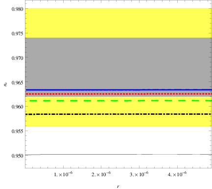
For , we have a positive value of but it still does not fall in the observational range as shown
in Fig. (1). As we increase the value of , the theoretical value of shifts towards the observed value.
From Fig. (1) it is clear that for and , there exist no values of for which lies in this
range at the confidence level. However for , and , (Fig. (2)) the value
of given by the theoretical model agrees with the Planck 2015 results up to the
confidence level. Interesting results are found for and for which the plots
are shown in Fig. (1). For , and
, (Fig. (2)) the theoretical value of the spectral index is in agreement with the Planck 2015 data
up-to the confidence level. For , we have whereas
, for and . For higher value of , becomes much smaller than
and also the spectral index attains a constant value of
and respectively for and . The tensor-to-scalar ratio satisfies the Planck
2015 data [33], i.e., for all the values of discussed here.
We should emphasize that the permitted range of parameters in the model leads to small numerical values of , thereby, the Lyth bound [34] is easily satisfied in the sub-Planckian region. Indeed, using Eq. (11),
| (26) |
As is a monotonically increasing function in the model under consideration, and the range of inflation is given by, . For , , we find that and Lyth bound is satisfied as stated.


III Preheating based upon instant particle production
In the paradigm of quintessential inflation, the underlying potential is typically of a run away type. Thereby the standard mechanism of (p)reheating[35, 36, 37, 38] can not be implemented in this case. One of the possible alternatives is provided by gravitational particle production. However, this process is inefficient and as a result the field spends a long time in the kinetic regime (). The energy density of gravity waves which were produced at the end of inflation becomes sufficiently larger than during the kinetic regime and this leads to a violation of the nucleosynthesis constraint. The nucleosynthesis constraint restricts the duration of the kinetic regime and we can also put a lower bound on the reheating temperature using this constraint. Therefore, we require an efficient reheating mechanism to address the issue. The instant preheating mechanism turns out to be suitable.
In what follows, we shall consider a scenario where the inflaton field interacts with another scalar field and we assume that the scalar field interacts with the matter field such that[39],
| (27) |
Let us choose the following interaction terms in the Lagrangian,
| (28) |
in order to implement the aforesaid. Here and are positive coupling constants [40, 41, 42, 43, 34]. The form of the Lagrangian is chosen such that field has no bare mass and its effective mass is given by [44]. Particle production commences after inflation provided that changes non-adiabatically, . The mass of produced particles grows as the field evolves to larger values after the end of inflation and decays into various species of particles. Assuming that all the energy is instantaneously converted into radiation and thermalized, one can obtain the following estimate(see Appendix A for details),
| (29) |
As mentioned before, the energy density of gravity waves becomes significantly larger than during the kinetic regime and this might later lead to a violation of the nucleosynthesis constraint during the radiative regime. The said constraint,
| (30) |
where, combined with the value of the dimensionless gravity wave amplitude calculated for our model (see appendix A) puts an upper bound on ,
| (31) |
at the end of inflation. This gives us a lower bound on , and hence a bound on the reheating temperature, , is obtained. Using Eq. (29) together with Eq. (31), we find out the lower limit on . The limit on can be set by avoiding the back reaction of particles on the post inflationary dynamics. We find a comfortable range in the parameter space which can give rise to efficient preheating after inflation (see Appendix A for details).
IV Late time acceleration with non-minimal coupling to massive neutrino matter
In the absence of non-minimal coupling, the scalar field with a potential given by Eq. (2) can not give rise to late time acceleration as the potential is steep. To obtain late time acceleration one needs to introduce a feature in the potential which can be achieved by coupling the scalar field non minimally to massive neutrino matter. The coupling of the scalar field with neutrinos is not prominent in the radiation era while it plays a crucial role during the late stages of evolution where it induces a minimum in the potential giving rise to a de Sitter solution. The result is a late time attractor. As mentioned before, it is desirable to leave the matter era intact and assume that the field couples to massive neutrino matter only.
The neutrinos here are relativistic like radiation during early times but turn non relativistic at late times. This behaviour can be mimicked by the following ansatz for parametrization of ,
| (32) |
The equation of state is thus chosen keeping in mind the phase transition from the relativistic state to the non relativistic one. and give the time and duration of the transition. The equation of continuity for massive neutrinos, in presence of coupling, takes the form, [23, 34].
| (33) |
Varying the action (1) with respect to and following the Ref. [34], we obtain,
| (34) |
We note that in the radiation era when the neutrino is relativistic, in Eqs (33) and (34), the coupling term of the scalar field and neutrinos vanishes since . Thus the coupling becomes effective only when the neutrinos become non-relativistic. We thus have a system of equations,
| (35) |
| (36) |
| (37) |
| (38) |
| (39) |
which we can solve to obtain the evolution of the various energy densities. To solve this system of differential equations, we introduce the dimensionless variables , , , , and where , , , , and . The evolution equations can then be cast in a convenient form,
| (41) | |||||
| (42) | |||||
| (43) | |||||
| (44) | |||||
| (45) |
Here, prime ′ is derivative w.r. to and we have used the constraint, .
We now solve this dynamical system numerically for and plot
these variables taking the initial conditions at the end of inflation. The initial values of , , , and
are approximately , , , , and respectively.
and are and respectively. The initial value of is . From the plots of
Fig. (3), it is clear that we can obtain late time acceleration with neutrino coupling using
these initial conditions, since we can obtain the current values of , and which
are approximately , and respectively. Similar graphs were plotted for etc. and the same result was obtained.
A comment regarding the thawing nature of evolution is in order. The potential (2) belongs to the
class of tracker potentials.
Indeed, One can easily check that our potential behaves as [45] asymptotically for large values of . However, on the contrary, we see a thawing behaviour. It is clear from subfigure (3d) that after inflation ends, the potential drops sharply resulting in a deep overshoot of with respect to the background energy density. Clearly, it takes long time for the field to recover from freezing which happens when the background energy density become comparable to . When it happens, the field has already evolved to the slow roll regime near the minimum of the potential and consequently, tracker regime is missed out.
In this case nucleosynthesis poses no constraint on the slope of the potential unlike the case of standard exponential potential.
V Conclusions
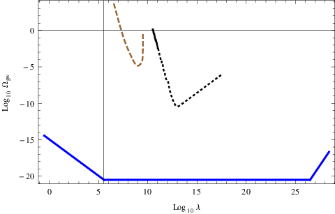
In this paper, we have considered a single scalar field model with a potential and demonstrated that the model can give rise to quintessential inflation. First, we have demonstrated the viability of the theory for inflation. In particular, we have shown that for lower values of , the model is ruled out by observation. For instance if , the theoretical value of fails to lie in the observed range. However, situation improves for higher values of ; potential flattens significantly in this case. In particular, for and , the considered potential provides a value of such that it can lie in the range of confidence level of Planck 2015 data. The value of is greater than and for and respectively. The most profound results are obtained for and . The theoretical value of satisfies the Planck 2015 data at the confidence level and its value becomes and for and for and respectively. It should be noted that our model mimics the hill-top potential [32] for as . It is therefore not surprising that the tensor-to-scalar ratio is negligibly small in our case similar to that of the Starobinsky-model [46]. Nevertheless, the very small value of the tensor-to-scalar ratio is a salient feature of our model compared to other models discussed in the literature. If we take to be much less than unity, we find that the value of is significantly greater than . Further, we have plotted the evolution of normalized values of different components of the energy densities , , and the energy density of the scalar field . The plots explain that the universe undergoes late time acceleration, i.e., for today, , and . Though the underlying potential belongs to the tracker class, the thawing behaviour manifests itself in the post-inflationary region. This behaviour depends on the specific initial conditions taken at the end of inflation. The latter then leads to a deep overshoot of the field and consequently misses the tracker region of the potential. Thus, in the model under consideration (in a thawing realization), the scalar field which drives inflation in the early Universe is also responsible for late time acceleration once we couple the scalar field to massive neutrino matter. Finally, we considered the instant preheating mechanism for particle production where we assumed that the scalar field couples to the matter field via Yukawa interaction. We have put bounds on the coupling constants and defined in the Yukawa interaction which are found to be and such that . These values satisfy the nucleosynthesis constraint. We have also studied the spectrum of relic gravity waves in our model (see appendix B); the generic feature of the scenario includes the blue spectrum of gravity waves on scales smaller than comoving horizon scales. Fig. (4) shows the energy spectrum for and as a function of the wavelength together with the sensitivity curves of advLIGO and LISA.
Acknowledgement
Naveen K. Singh is thankful to the D.S. Kothari postdoctoral fellowship of University Grant Commission, India for the financial support. His fellowship number is F.4-2/2006 (BSR)/PH/14-15/0034. Abhineet Agarwal wishes to thank Md. Wali Hossain and Safia Ahmad for useful discussions.
Appendices
Chapter \thechapter Appendix A: Instant preheating
In order to implement the instant particle production, we consider the following Lagrangian,
| (46) |
where and are positive coupling constants with a restriction, such that a perturbative treatment is viable for the Lagrangian (46) [40, 41, 42, 43, 34]. The effective mass of can be read of from (46) as, , [44]. Production of particles takes place after inflation provided changes non adiabatically, [16, 43, 34, 40]
| (47) |
Let us now confirm that the above condition is met in the model under consideration. To this effect, we estimate using the expression of slow roll parameter, ,
| (48) |
The condition for particle production then becomes,
| (49) |
Using Eq. (49), we have following expression,
The production time can be estimated[43, 34, 40, 37, 38] as
| (50) |
which allows us then to estimate wave number using uncertainty relation,
| (51) |
The occupation number for particles is given by the following expression,
| (52) |
We can then find the number density and energy density of created particles,
| (53) |
| (54) |
Now plugging in the above equation, one finds,
| (55) |
Substituting in the above equation, reduces to
| (56) |
Using Eq. (48) and ,
| (57) |
Combining Eq. (55) and Eq. (57) yields,
| (58) |
Assuming that the field gets converted into radiation and thermalization takes place instantaneously, we have,
| (59) |
We thus obtain,
| (60) |
The nucleosynthesis constraint [34] dictates that
| (61) |
where
| (62) |
Combining and with Eq. (57), Eq. (61) and Eq. (62), one obtains the following inequality,
| (63) |
Considering the form of our potential at the beginning and end of inflation, the above inequality reduces to,
| (64) |
Using together with , and , where these values are obtained for and , the following bound on is calculated,
| (65) |
Using , the bound on can be written as
| (66) |
Using Eq. (57), the inequality Eq. (63) can be rewritten as
| (67) |
Evaluating the expression on the right hand side for and as above, the above inequality is calculated as,
| (68) |
Plugging Eq. (60) in Eq. (68), we obtain the bound on ,
| (69) |
We now calculate the bound on . For the reaction, , the decay width satisfies the following inequality [35, 36, 37, 38, 34, 43, 40, 42, 39, 47, 41, 44, 16],
| (70) |
Now using , Eq. (57) and for our potential one obtains
| (71) |
which simplifies to
| (72) |
for and . From Eq. (69), can take any value greater than or equal to and based on the value taken by , satisfies Eq. (72). The bounds on and that are calculated above are such that always satisfies the inequality (66).
Chapter \thechapter Appendix B: Relic Gravity Wave Spectrum
One of the tests for inflationary models is the measurement of the spectrum of gravity waves. In this appendix, considering the given reheating temperature, we estimate the spectrum of the relic gravity wave. The gravitational wave equation in flat FRW space time can be written in its standard form as,
| (73) |
This equation describes how gravity wave evolves with time in a flat FRW Universe. The energy spectrum is defined as [48],
| (74) |
where and the gravitational energy density is given by
| (75) |
It can be shown that the spectrum of gravity waves depends on the equation of state of the dominant fluid comprising the universe [24, 48]. Therefore, the gravitational waves can be categorized according to three epochs of the universe - the matter dominated regime, the radiation dominated regime and the kinetic regime, and in these regimes the energy spectrum of relic gravity waves is given by the following expressions [24]:
| (76) | |||||
| (77) | |||||
| (78) |
where, . , can be estimated using the boundary conditions: and . So, we have,
| (79) | ||||
| (80) |
and is given by
| (81) |
The gravity waves with wavelength are generated during the kinetic regime (). The spectrum of these waves is inversely proportional to the wavelength. During the radiation phase, , it is constant. However, for , the waves are created in the matter phase and its spectrum increases according to Eq. (76). Now we calculate , and .
| (82) |
Here, we plugged and for and respectively.
| (83) |
where, we used and .
| (84) |
Using and we get,
| (85) |
We have , , , ,
| (86) |
Substituting , and in Eq. (85), turns out to be,
| (87) |
Now using and one obtains,
| (88) |
Using , , and , can be written as
| (89) |
which simplifies Eqs. (76), (77) and (78) as following,
| (90) | ||||
| (91) | ||||
| (92) |
References
- [1] A. H. Guth, Phys. Rev. D 23, 347 (1981).
- [2] A. A. Starobinsky, Phys. Lett. 91B, 99 (1980).
- [3] A. A. Starobinsky, Phys. Lett. B117, 175 (1982).
- [4] A. D. Linde, Phys. Lett. B129, 177 (1983).
- [5] A. D. Linde, Phys. Lett. B108, 389 (1982).
- [6] M. Gasperini and M. Giovannini, Phys. Lett. B 282, 36 (1992).
- [7] D. H. Lyth and A. Riotto, Phys. Rept. 314, 1 (1999) [hep-ph/9807278].
- [8] S. Perlmutter et al. [Supernova Cosmology Project Collaboration], Astrophys. J. 517, 565 (1999) [astro-ph/9812133].
- [9] A. G. Riess et al., Astron. J. 117, 707 (1999) [astro-ph/9810291].
- [10] P. J. E. Peebles and A. Vilenkin, Phys. Rev. D 59, 063505 (1999) [astro-ph/9810509].
- [11] S. Dodelson and L. Knox, Phys. Rev. Lett. 84, 3523 (2000) [astro-ph/9909454].
- [12] M. S. Turner, Phys. Scripta T 85, 210 (2000) [astro-ph/9901109].
- [13] L. Amendola and D. Tocchini-Valentini, Phys. Rev. D 64, 043509 (2001) [astro-ph/0011243].
- [14] R. R. Caldwell, Phys. Lett. B 545, 23 (2002) [astro-ph/9908168].
- [15] P. J. E. Peebles and B. Ratra, Rev. Mod. Phys. 75, 559 (2003) [astro-ph/0207347].
- [16] M. Sami and V. Sahni, Phys. Rev. D 70, 083513 (2004) [hep-th/0402086].
- [17] E. J. Copeland, M. Sami and S. Tsujikawa, Int. J. Mod. Phys. D 15, 1753 (2006) [hep-th/0603057].
- [18] L. M. Krauss and M. S. Turner, Gen. Rel. Grav. 27, 1137 (1995) [astro-ph/9504003].
- [19] M. Giovannini, Class. Quant. Grav. 16, 2905 (1999) [hep-ph/9903263].
- [20] M. Giovannini, Phys. Rev. D 60, 123511 (1999) [astro-ph/9903004].
- [21] M. Giovannini, Phys. Rev. D 67, 123512 (2003) [hep-ph/0301264].
- [22] P. J. Steinhardt, L. M. Wang and I. Zlatev, Phys. Rev. D 59, 123504 (1999) [astro-ph/9812313].
- [23] C. Q. Geng, M. W. Hossain, R. Myrzakulov, M. Sami and E. N. Saridakis, Phys. Rev. D 92, no. 2, 023522 (2015) [arXiv:1502.03597 [gr-qc]].
- [24] V. Sahni, M. Sami and T. Souradeep, Phys. Rev. D 65, 023518 (2002) [gr-qc/0105121].
- [25] S. Weinberg, The Cosmological constant problems, in Sources and detection of dark matter and dark energy in the universe. Proceedings, 4th International Symposium, DM 2000, Marina del Rey, USA, February 23-25, 2000 astro-ph/0005265.
- [26] M. W. Hossain, R. Myrzakulov, M. Sami and E. N. Saridakis, Phys. Rev. D 90, no. 2, 023512 (2014) [arXiv:1402.6661 [gr-qc]].
- [27] L. Amendola, M. Baldi and C. Wetterich, Phys. Rev. D 78, 023015 (2008) [arXiv:0706.3064 [astro-ph]].
- [28] N. D. Lambert, H. Liu and J. M. Maldacena, JHEP 0703, 014 (2007) [hep-th/0303139].
- [29] G. S. Djordjevic, D. D. Dimitrijevic and M. Milosevic, Rom. J. Phys. 61, no. 1-2, 99 (2016).
- [30] A. Sen, “NonBPS states and Branes in string theory,” in Supersymmetry in the theories of fields, strings and branes. Proceedings, Advanced School, Santiago de Compostela, Spain, July 26-31,1999, pp. 187-234, 1999 hep-th/9904207.
- [31] A. Sen, JHEP 0204, 048 (2002) [hep-th/0203211].
- [32] L. Boubekeur and D. H. Lyth, JCAP 0507, 010 (2005) [hep-ph/0502047].
- [33] P. A. R. Ade et al. [Planck Collaboration], Astron. Astrophys. 594, A20 (2016) [arXiv:1502.02114 [astro-ph.CO]].
- [34] M. Wali Hossain, R. Myrzakulov, M. Sami and E. N. Saridakis, Int. J. Mod. Phys. D 24, no. 05, 1530014 (2015) doi:10.1142/S0218271815300141 [arXiv:1410.6100 [gr-qc]].
- [35] D. H. Lyth, A.R. Liddle and R. Andrew, editors, “THE PRIMORDIAL DENSITY PERTURBATION; Cosmology, Inflation and the Origin of Structure,” Cambridge University Press, 2009.
- [36] P. Binetruy , R. Schaeffer , J. Silk and F. David, editors, “The Primordial Universe,” EDP Sciences, Springer - Verlag, 2000.
- [37] L. Kofman, A. D. Linde and A. A. Starobinsky, Phys. Rev. D 56, 3258 (1997) [hep-ph/9704452].
- [38] L. Kofman, A. D. Linde and A. A. Starobinsky, Phys. Rev. Lett. 73, 3195 (1994) [hep-th/9405187].
- [39] A. H. Campos, J. M. F. Maia and R. Rosenfeld, Phys. Rev. D 70, 023003 (2004) [astro-ph/0402413].
- [40] M. Sami and N. Dadhich, TSPU Bulletin 44N7, 25 (2004) [hep-th/0405016].
- [41] G. N. Felder, L. Kofman and A. D. Linde, Phys. Rev. D 59, 123523 (1999) [hep-ph/9812289].
- [42] S. Tsujikawa, B. A. Bassett and F. Viniegra, JHEP 0008, 019 (2000) doi:10.1088/1126-6708/2000/08/019 [hep-ph/0006354].
- [43] M. W. Hossain, R. Myrzakulov, M. Sami and E. N. Saridakis, Phys. Rev. D 90, no. 2, 023512 (2014) [arXiv:1402.6661 [gr-qc]].
- [44] G. N. Felder, L. Kofman and A. D. Linde, Phys. Rev. D 60, 103505 (1999) [hep-ph/9903350].
- [45] C. Q. Geng, C. C. Lee, M. Sami, E. N. Saridakis and A. A. Starobinsky, JCAP 1706, no. 06, 011 (2017) doi:10.1088/1475-7516/2017/06/011 [arXiv:1705.01329 [gr-qc]].
- [46] A. A. Starobinsky, Phys. Lett. 91B, 99 (1980).
- [47] A. H. Campos, H. C. Reis and R. Rosenfeld, Phys. Lett. B 575, 151 (2003) [hep-ph/0210152].
- [48] L. A. Boyle and P. J. Steinhardt, Phys. Rev. D 77, 063504 (2008) [astro-ph/0512014].