Statistics on the (compact) Stiefel manifold: Theory and Applications
Abstract
A Stiefel manifold of the compact type is often encountered in many fields of Engineering including, signal and image processing, machine learning, numerical optimization and others. The Stiefel manifold is a Riemannian homogeneous space but not a symmetric space. In previous work, researchers have defined probability distributions on symmetric spaces and performed statistical analysis of data residing in these spaces. In this paper, we present original work involving definition of Gaussian distributions on a homogeneous space and show that the maximum-likelihood estimate of the location parameter of a Gaussian distribution on the homogeneous space yields the Fréchet mean (FM) of the samples drawn from this distribution. Further, we present an algorithm to sample from the Gaussian distribution on the Stiefel manifold and recursively compute the FM of these samples. We also prove the weak consistency of this recursive FM estimator. Several synthetic and real data experiments are then presented, demonstrating the superior computational performance of this estimator over the gradient descent based non-recursive counter part as well as the stochastic gradient descent based method prevalent in literature.
1 Introduction
Manifold-valued data have gained much importance in recent times due to their expressiveness and ready availability of machines with powerful CPUs and large storage. For example, these data arise as rank-2 tensors (manifold of symmetric positive definite matrices) [36, 39], linear subspaces (the Grassmann manifold) [50, 26, 23, 37], column orthogonal matrices (the Stiefel manifold) [50, 28, 14], directional data and probability densities (the hypersphere) [34, 47, 49, 25] and others. A useful method of analyzing manifold valued data is to compute statistics on the underlying manifold. The most popular statistic is a summary of the data, i.e., the Riemannian barycenter (Fréchet mean (FM)) [22, 31, 2], Fréchet median [4, 11] etc. However, in order to compute statistics of manifold-valued data, the first step involves defining a distribution on the manifold. Recently, authors in [44] have defined a Gaussian distribution on Riemannian symmetric spaces (or symmetric spaces). Some typical examples of symmetric spaces include the Grassmannian, the hypersphere etc. Several other researchers [13, 43] have defined a Gaussian distribution on the space of symmetric positive definite matrices. They called the distribution a “generalized Gaussian distribution” [13] and “Riemannian Gaussian distribution” [43] respectively.
In this work, we define a Gaussian distribution on a homogeneous space (a more general class than symmetric spaces). A key difficulty in defining the Gaussian distribution on a non-Euclidean space is to show that the normalizing factor in the expression for the distribution is a constant. In this work, we show that the normalizing factor in our definition of the Gaussian distribution on a homogeneous space is indeed a constant. Note that a symmetric space is a homogeneous space but not all homogeneous spaces are symmetric and thus, our definition of Gaussian distribution is on a more generalized topological space than the symmetric space. Given a well-defined Gaussian distribution, the next step is to estimate the parameters of the distribution. In this work, we prove that the maximum likelihood estimate (MLE) of the mean of the Gaussian distribution is the Fréchet mean (FM) of the samples drawn from the distribution.
Data with values in the space of column orthogonal matrices have become popular in many applications of Computer Vision and Medical Image analysis [50, 9, 33, 8, 40]. The space of column orthogonal matrices is a topological space, and moreover one can equip this space with a Riemannian metric which in turn makes this space a Riemannian manifold, known as the Stiefel manifold. The Stiefel manifold is a homogeneous space and here we extend the definition of the Gaussian distribution to the Stiefel manifold. In this work, we restrict ourselves to the Stiefel manifold of the compact type, which is quite commonly encountered in most applications mentioned earlier.
We now motivate the need for a recursive FM estimator. In this age of massive and continuous streaming data, samples are often acquired incrementally. Hence, from an applications perspective, the desired algorithm should be recursive/inductive in order to maximize computational efficiency and account for availability of data, requirements that are seldom addressed in more theoretically oriented fields. We propose an inductive FM computation algorithm and prove the weak consistency of our proposed estimator. FM computation on Riemannian manifolds has been an active area of research for the past few decades. Several researchers have addressed this problem and we refer the reader to [6, 2, 24, 38, 3, 35, 5, 41, 19, 4, 48, 29, 10, 45].
1.1 Key Contributions
In summary, the key contributions of this paper are: (i) A novel generalization of Gaussian distributions to homogeneous spaces. (ii) A proof that the MLE of the location parameter of this distribution is “the” FM. (iii) A sampling technique for drawing samples from this generalized Gaussian distribution defined on a compact Stiefel manifold (which is a homogeneous space), and an inductive/recursive FM estimator from the drawn samples along with a proof of its weak consistency. Several examples of FM estimates computed from real and synthetic data are shown to illustrate the power of the proposed methods.
Though researchers have defined Gaussian distributions on other manifolds in the past, see [44, 13], their generalization of the Gaussian distribution is restricted to symmetric spaces of non-compact types. In this work, we define a Gaussian distribution on a homogeneous space, which is a more general topological space than the symmetric space. A few others in literature have generalized the Gaussian distribution to all Riemannian manifolds, for instance, in [52], authors defined the Gaussian distribution on a Riemannian manifold without a proof to show that the normalizing factor is a constant. Whereas, in [38], the author defined the normal law on Riemannian manifolds using the concept of entropy maximization for distributions with known mean and covariance. Under certain assumptions, the author shows that this definition amounts to using the Riemannian exponential map on a truncated Gaussian distribution defined in the tangent space at the known intrinsic mean. This approach of deriving the normal distribution yields a normalizing factor that is dependent on the location parameter of the distribution and hence is not a constant with respect to the FM. To the best of our knowledge, we are the first to define a Gaussian distribution on a homogeneous space with a constant normalizing factor, i.e., the normalizing factor does not depend on the location parameter (FM).
We then move our focus to the Stiefel manifold (which is a homogeneous space) and propose a simple algorithm to draw samples from the Gaussian distribution on the Stiefel manifold. In order to achieve this, we develop a simple but non-trivial way to extend the sampling algorithm in [44] to get samples on the Stiefel manifold. Once we have the samples from a Gaussian distribution on the Stiefel, we propose a novel estimator of the sample FM and prove the weak consistency of this estimator. The proposed FM estimator is inductive in nature and is motivated by the inductive FM algorithm on the Euclidean space. But, unlike Euclidean space, due to the presence of non-zero curvature, it is necessary to prove the consistency of our proposed estimator, which is presented subsequently. Further, we experimentally validate the superior performance of our proposed FM estimator over the gradient descent based techniques. Moreover, we also show that the MLE of the location parameter of the Gaussian distribution on the Stiefel manifold asymptotically achieves the Cramér-Rao lower bound [15, 42], hence in turn, the MLE of the location parameter is efficient. This implies that our proposed consistent FM estimator, asymptotically, has a variance lower bounded by that of the MLE.
The rest of the paper is organized as follows. In section 2, we present the necessary mathematical background. In section 3, we define a Gaussian distribution on a homogeneous space. More specifically, define a generalized Gaussian distribution on the Stiefel manifold and prove that the normalizing factor is indeed a constant with respect to the location parameter of the distribution. Then, we propose a sampling algorithm to draw samples from this generalized Gaussian distribution in section 3.1 and in section 3.2, show that the MLE of the location parameter of this Gaussian distribution is the FM of the samples drawn from the distribution. In section 4, we propose an inductive FM estimator and prove its weak consistency. Finally we present a set of synthetic and real data experiments in section 5 and draw conclusions in section 6.
2 Mathematical Background: Homogeneous spaces and the Riemannian symmetric space
In this section, we present a brief note on the differential geometry background required in the rest of the paper. For a detailed exposition on these concepts, we refer the reader to a comprehensive and excellent treatise on this topic by Helgason [27]. Several propositions and lemmas that are needed to prove the results in the rest of the paper are stated and proved here. Some of these might have been presented in the vast differential geometry literature but are unknown to us and hence the proofs presented in this background section are original.
Let be a Riemannian manifold with a Riemannian metric , i.e., is a bi-linear symmetric positive definite map, where is the tangent space of at . Let be the metric (distance) induced by the Riemannian metric . Let be the set of all isometries of , i.e., given , , for all . It is clear that forms a group (henceforth, we will denote by ) and thus, for a given and , , for some is a group action. Consider , and let , i.e., is the Stabilizer of . We say that acts transitively on , iff, given , there exists a such that .
Definition 2.1.
Let act transitively on and , (called the “origin” of ) be a subgroup of . Then, is a homogeneous space and can be identified with the quotient space under the diffeomorphic mapping [27].
In fact, if is a homogeneous space, then is a Lie group. A Stiefel manifold, (definition of the Stiefel manifold is given in next section) is a homogeneous space and can be identified with , where is the group of orthogonal matrices. Now, we will list some of the important properties of Homogeneous spaces that will be used throughout the rest of the paper.
Properties of Homogeneous spaces: Let be a Homogeneous space. Let be the corresponding volume form and be any integrable function. Let , s.t. , . Then, the following facts are true:
- 1.
.
- 2.
, for all .
- 3.
Definition 2.2.
A Riemannian symmetric space is a Riemannian manifold with the following property: such that and . is called symmetry at [27].
Proposition 2.1.
[27] A symmetric space is a homogeneous space with a symmetry, , at . For the other point , by transitivity of , there exists such that and .
Proposition 2.2.
[27] Any symmetric space is geodesically complete.
Some examples of symmetric spaces include, (the hypersphere), (the hyperbolic space) and (the Grassmannian). It is evident from the definition that symmetric space is a homogeneous space but the converse is not true. For example, the Stiefel manifold is not a symmetric space.
Proposition 2.3.
[27] The mapping is an involutive automorphism of and the stabilizer of , i.e., , is contained in the group of fixed points of .
Clearly, , as is an automorphism, is the identity element. Recall, is a Lie group, hence, differentiating at , we get an involutive automorphism of the Lie algebra of (also denoted by ). Henceforth, we will use to denote the automorphism of . Since is involutive, i.e., , has two eigen values, and let (Lie algebra of ) and be the corresponding eigenspaces, then (direct sum).
Proposition 2.4.
[27] , and
Hence, is a Lie subalgebra of . Henceforth, we will assume to be semisimple. We can define a symmetric, bilinear form, on as follows , where is the adjoint endomorphism of defined by . is called the Killing form on .
Definition 2.3.
The decomposition of as is called the Cartan decomposition of associated with the involution . Furthermore, is negative definite on , positive definite on and and are orthogonal complement of each other with respect to on .
Recall, a symmetric space, , can be identified with . Note that, , the “origin” of can be written as , is the identity element. Since, can be identified with , the Riemannian metric on corresponds to the Killing form on [27], which is a -invariant form. Without loss of generality, we will assume that is over and be semisimple (equivalently, the Killing form on is non-degenerate). The symmetric space is said to be compact (noncompact) iff the sectional curvature is strictly positive (negative), equivalently iff is compact (noncompact).
Duality: Given a semisimple Lie algebra with the Cartan decomposition , construct another Lie algebra from as follows: , where is a complex structure of (real Lie algebra). From the definition of complex structure, , is an automorphism on s.t., . satisfies the following equality: , for all . We will call the dual Lie algebra of . It is easy to see that if corresponds to a symmetric space of noncompact type, is a symmetric space of compact type and vice-versa. This duality property is very useful and is a key ingredient of this paper.
Now, we will briefly describe the geometry of two Riemannian manifolds, namely the Stiefel manifold and the Grassmannian. We need the geometry of Stiefel manifold throughout the rest of the paper. Furthermore, observe that, the Stiefel and the Grassmannian form a fiber bundle. In order to draw samples from a distribution on the Stiefel, we will use the samples drawn from a distribution on the Grassmannian by exploiting the fiber bundle structure. Hence, we will require the geometry of the Grassmannian as well, which we will briefly present below.
Differential Geometry of the Stiefel manifold: The set of all full column rank dimensional real matrices form a Stiefel manifold, , where . A compact Stiefel manifold is the set of all column orthonormal real matrices. When , can be identified with , where is special orthogonal group. Note that, when we consider the quotient space, , we assume that is a subgroup of , where, defined by is an isomorphism from to .
Proposition 2.5.
is a closed Lie-subgroup of . Moreover, the quotient space together with the projection map, is a principal bundle with as the fiber.
Proof.
is a compact Lie-subgroup of , hence is a closed subgroup. The fiber bundle structure of follows directly from the closedness of . As is a principal homogeneous space (because and acts on it freely), hence the principal bundle structure. ∎
With a slight abuse of notation, henceforth, we denote the compact Stiefel manifold by . Hence, , where is the identity matrix. The compact Stiefel manifold has dimension . At any , the tangent space is defined as follows . Now, given , the canonical Riemannian metric on is defined as follows:
| (2.1) |
With this metric, the compact Stiefel manifold has non-negative sectional curvature [53].
Given , we can define the Riemannian retraction and lifting map within an open neighbourhood of . We will use an efficient Cayley type retraction and lifting maps respectively on as defined in [21, 30]. It should be mentioned that though the domain of retraction is a subset of the domain of inverse-Exponential map, on retraction/ lifting is a useful alternative since, there are no closed form expressions for both the Exponential and the inverse-Exponential maps on Stiefel manifold. Recently, a fast iterative algorithm to compute Riemannian inverse-Exponential map has been proposed in [54], which can be used instead of retraction/ lifting maps to compute FM in our algorithm.
In the neighborhood of ( matrix with upper-right block is identity and rest are zeros), given , we define the lifting map by where, is a skew-symmetric matrix and is a matrix defined as follows: and where, , and with , and , provided that is nonsingular. is defined as and, .
Furthermore, in the neighborhood of , the retraction map defined above is a diffeomorphism (since it is a chart map) from to .
Proposition 2.6.
The projection map is a covering map on the neighborhood of in .
Proof.
First, note that under the identification of with , the neighborhood of in can be identified with the neighborhood of in . Now, the retraction map defined above is a (local) diffeomorphism from to . Also, the Cayley map is a diffeomorphism from to the neighborhood of in . Thus, the map is a diffeomorphism to the neighborhood of in (using the fact that the composition of two diffeomorphisms is a diffeomorphism). Now, since is compact and is surjective, is a covering map on the neighborhood of in using the following Lemma. ∎
Lemma 2.1.
Under the hypothesis in Proposition 2.6, is a covering map in the neighborhood from the neighborhood of in to the neighborhood of of .
Proof.
In Proposition 2.6, we have shown that is local diffeomorphism in the neighborhood specified in the hypothesis. Let be a neighborhood around in and be a neighborhood around in on which is a diffeomorphism. Let , as is a space, hence, is closed, thus, is closed and since is compact, hence is compact. For each , let be a open neighborhood around where restricts to a diffeomorphism (and hence homeomorphism). Then, is an open cover of , thus as a finite subcover , where is finite. We chose to be disjoint as is a space. Let which is an open neighborhood of . Then, is a disjoint collection of open neighborhoods each of which maps homeomorphically to . Hence, is a covering map in the local neighborhood. ∎
Given , the Cayley map is a conformal mapping, defined by . Using the Cayley mapping, we can define the Riemannian retraction map by . Hence, given within a regular geodesic ball (the geodesic ball does not include the cut locus) of appropriate radius (henceforth, we will assume the geodesic ball to be regular), we can define the unique geodesic from to , denoted by as
| (2.2) |
Also, we can define the distance between and as
| (2.3) |
Differential Geometry of the Grassmannian : The Grassmann manifold (or the Grassmannian) is defined as the set of all -dimensional linear subspaces in and is denoted by , where , , . Grassmannian is a symmetric space and can be identified with the quotient space , where is the set of all matrices whose top left and bottom right submatrices are orthogonal and all other entries are , and overall the determinant is . A point can be specified by a basis, . We say that if is a basis of , where is the column span operator. It is easy to see that the general linear group acts isometrically, freely and properly on . Moreover, can be identified with the quotient space . Hence, the projection map is a Riemannian submersion, where . Moreover, the triplet is a fiber bundle.
At every point , we can define the vertical space, to be . Further, given , we define the horizontal space, to be the -orthogonal complement of . Now, from the theory of principal bundles, for every vector field on , we define the horizontal lift of to be the unique vector field on for which and , . As, is a Riemannian submersion, the isomorphism is an isometry from to . So, is defined as:
| (2.4) |
where, and , , and .
3 Gaussian distribution on Homogeneous spaces
In this section, we define the Gaussian distribution, on a Homogeneous space, , (location parameter), (scale parameter), and then propose a sampling algorithm to draw samples from the Gaussian distribution on . Furthermore, we will show that the maximum likelihood estimator (MLE) of is the Fréchet mean (FM) [22] of the samples.
We define the probability density function, with respect to (the volume form) of the Gaussian distribution on as:
| (3.1) |
The above is a valid probability density function, provided the normalizing factor, is a constant, i.e., does not depend on which we will prove next.
Proposition 3.1.
Let us define . Then, , where is the origin.
Proof.
As the group action on is transitive, there exists s.t., .
Hence, , i.e., does not depend on . ∎
Now that we have a valid definition of a Gaussian distribution, on a Homogeneous space, we propose a sampling algorithm for drawing samples from on (which is a homogeneous space), .
3.1 Sampling algorithm
In order to draw samples from on , it is sufficient to draw samples from where is the origin. Then, using group operation, we can draw samples from for any . We will assume, ( matrix with the upper-right block being the identity and the rest being zeros). We will first draw samples from on , where and use this sample to get a sample on using . Note that is a symmetric space and hence a homogeneous space and thus we have a valid Gaussian density on using Eq. 3.1.
Proposition 3.2.
Let where , . Then, , with , where, and .
Proof.
It is sufficient to show that . Recall, that forms a fiber bundle. Moreover, the isomorphism, is an isometry from to , for all . From, [1], we know that . So,
∎
Using the Proposition 3.2, we can generate a sample from on , using a sample from on . We will now propose an algorithm to draw samples from on . Recall that can be identified as which is a semisimple symmetric space of compact type (let it be denoted by ). Also, recall from section 2 that, every compact semisimple symmetric space has a dual semsimple symmetric space of non-compact type (denoted by ). Here, , , where , , , . Then, , and the corresponding Lie group, denoted by (with a slight abuse of notation we use to denote the identity component). Here, is the special pseudo-orthogonal group, i.e.,
,
. Thus, the dual non-compact type symmetric space of (identified with ) is . Recently, in [44], an algorithm to draw samples from a Gaussian distribution on symmetric spaces of non-compact type was presented. We will use the following proposition to get a sample from a Gaussian distribution on the dual compact symmetric space.
Proposition 3.3.
Let . Let , where Ad is the adjoint representation, , . Then, , where and .
Proof.
Observe that . So, it suffices to show that .
∎
Note that, the mapping given by is a diffeomorphism and is used to construct from . The mapping is called the polar coordinate transform. Now, using Propositions 3.2 and 3.3, starting with a sample drawn from a Gaussian distribution on , we get a sample from Gaussian distribution on . We would like to point out that, we do not have to compute the normalizing constant explicitly in order to draw samples, because, in order to get samples on , we can draw samples using the Algorithm 1 in [44], which draws samples from the kernel of the density.
3.2 Maximum likelihood estimation (MLE) of
Let, be i.i.d. samples drawn from with bounded support (described subsequently) on , for some . Then, by proposition 3.5, the MLE of is the Fréchet mean (FM) [22] of . Fréchet mean (FM) [22] of is defined as follows:
| (3.2) |
We define an (open) “geodesic ball” of radius to be s.t., there exists a length minimizing geodesic between to any . A “geodesic ball” is said to be “regular” iff , where is the maximum sectional curvature. The existence and uniqueness of the Fréchet mean (FM) is ensured iff the support of the distribution is within a regular geodesic ball [2, 32].
Proposition 3.4.
Let , , then,
Proof.
Observe that, the support of as defined in proposition 3.2 is a subset of , is an arbitrary union of open sets and hence is open. Thus, we can give a manifold structure and using the proposition 3.4, we can say that if the support of is within a geodesic ball , FM exists and is unique. For the rest of the paper, we assume this condition to ensure the existence and uniqueness of FM.
Proposition 3.5.
Let, be i.i.d. samples drawn from on (support of is within a geodesic ball ), . Then the MLE of is the FM of .
4 Inductive Fréchet mean on the Stiefel manifold
In this section, we present an inductive formulation for computing the Fréchet mean (FM) [22, 31] on Stiefel manifold. We also prove the Weak Consistency of our FM estimator on the Stiefel manifold.
Algorithm for Inductive Fréchet Mean Estimator
Let , , be i.i.d. samples drawn from
(whose support is within a geodesic
ball ) on . Then, we define the inductive FM estimator (StiFME)
by the recursion in Eqs. 4.1, 4.2.
(4.1)
(4.2)
where, is the
geodesic from to defined as and . Eq. 4.2 simply means that the
estimator lies on the geodesic between the estimate and the sample point. This simple inductive estimator can be shown to converge
to the Fréchet expectation, i.e., , as stated in Theorem
4.1.
Theorem 4.1.
Let, be i.i.d. samples drawn from a Gaussian distribution on (with a support inside a regular geodesic ball of radius ). Then the inductive FM estimator (StiFME) of these samples, i.e., converges to as .
Proof.
We will start by first stating the following propositions.
Proposition 4.1.
Proposition 4.2.
Let, , where and . Let, is an defined in Eq. 3.2, then, , where .
Proof.
Let, , for some . Then, observe that,
Thus the claim holds. ∎
Theorem 4.2.
Using the hypothesis in Theorem 4.1, let be the corresponding i.i.d. samples drawn from the (induced) Gaussian distribution on where () (it is easy to show using Proposition 4.2 that this (induced) distribution on is indeed a Gaussian distribution on ). Then the inductive FM estimator (StiFME) of these samples, i.e., converges to as .
Proof.
Since is a special case of the (compact) Stiefel manifold, i.e., when (as can be identified with ), we will use instead of for notational simplicity. Let . Any point in can be written as a product of planar rotation matrices by the following claim.
Proposition 4.3.
Any arbitrary element of can be written as the composition of planar rotations in the planes generated by the standard orthogonal basis vectors of .
Proof.
The proof is straightforward. Moreover, each element of is a product of planar rotations. ∎
By virtue of the Proposition 4.3, we can express as a product of planar rotation matrices. Each planar rotation matrix can be mapped onto , hence . Let’s denote this product space of hyperspheres by . Then, is a diffeomorphism from to . Let be a Riemannian metric on . Let be the Levi-Civita connection on . Since, is a diffeomorphism, every vector field on pushes forward to a well-defined vector field on . Define a map
, where gives the section of .
Proposition 4.4.
is the Levi-Civita connection on equipped with the pull-back Riemannian metric .
Proposition 4.5.
Given the hypothesis and the notation as above, if is a geodesic on , is a geodesic on .
Proof.
Let, be a curve in . Then,
Hence, is a geodesic on . ∎
Now, analogous to Eq. 4.1, we can define the FM estimator on where the geodesic, . Note that, on , .
Proposition 4.6.
Proof.
Let, and . Using Proposition 4.6, we get,
Thus, in order to show weak consistency of our proposed estimator on , it is sufficient to show the weak consistency of our estimator on . A proof of the weak consistency of our proposed FM estimator on hypersphere has been shown in [45] (which can be trivially extended to the product of hyperspheres). This proof of weak consistency on the hypersphere in turn proves the weak consistency on . ∎
Since we have now shown that our proposed FM estimator on is (weakly) consistent, we claim that, as , where is the MLE of when are i.i.d. samples from on . The following porposition computes the Fisher information of when samples are drawn from on .
Proposition 4.7.
Let be a random variable which follows on . Then,
Proof.
The likelihood of is given by
| (4.3) |
Then, , where is the log likelihood. Now, , hence, . Now, observe that, (here, definition of variance of a manifold valued random variable is as in [38]), where from the definition of the Gaussian distribution, . Hence, . ∎
As, (as we have shown that is the FM of the samples in proposition 3.5) when the number of samples tends to infinity, and by proposition 4.7, we conclude that MLE achieves the Cramér-Rao lower bound asymptotically (this observation is in line with normal random vector). Furthermore MLE is unbiased, and is asymptotically an efficient estiamtor. As, we have shown consistency of our estimator, hence is lower bounded by as . In other words, asymptotically, = .
5 Experimental Results
In this section, we present experiments demonstrating the performance of StiFME in comparison to the batch mode counterpart with “warm start”(which uses the gradient descent on the sum of squared geodesic distances cost function, henceforth termed StFME) on synthetic and real datasets. By “warm start” we mean that, when a new data point is acquired as input, we initialize the FM to its computed value prior to the arrival/acquisition of the new data point. All the experimental results reported here were performed on a desktop with a 3.33 GHz Intel-i7 CPU with 24 GB RAM.
5.1 Comparative performance of StiFME on Synthetic data
We generated i.i.d. samples drawn from a Normal distribution on with variance and expectation , where
We input these i.i.d. samples to both StiFME and StFME. To compare the performance, we compute the error, which is the distance (on ) between the computed FM and the known true FM . We also report the computation time for both these cases. We performed this experiment times and report the average error and the average computation time. The comparison plot for the average error is shown in Fig. 1, here , . In order to achieve faster convergence of StFME, we used the “warm start” technique, i.e., FM of samples is used to initialize the FM computation for samples. From this plot, it is evident that the average accuracy error of StiFME is almost same as that of StFME.
The computation time comparison between StiFME and StFME is shown in Fig. 1. From this figure, we can see that StiFME outperforms StFME. As the number of samples increases, the computational efficiency of StiFME over StFME becomes significantly large. We can also see that the time requirement for StiFME is almost constant with respect to the the number of samples, which makes StiFME computationally very efficient and attractive for large number of data samples.
Another interesting question to ask is, how much computation time is needed in order to estimate the FM with a given error tolerance? We answer this question through the plot in Figure 1 and present a comparison of the time required for StiFME and StFME respectively to reach the specified error tolerance. From Fig.1, is is evident that the time required to reach the specified error tolerance by StiFME is far less than that required by StFME.
5.2 Clustering action data from videos
In this subsection, we applied our FM estimator to cluster the KTH video action data [46].
| Method | Scenario | Precision(%) | Time(s) |
|---|---|---|---|
| StFME | d1 | ||
| StiFME | d1 | ||
| StFME | d2 | ||
| StiFME | d2 | ||
| StFME | d3 | ||
| StiFME | d3 | ||
| StFME | d4 | ||
| StiFME | d4 |
This data contains actions performed by human subjects in scenarios (denoted by ‘d1’, ‘d2’, ‘d3’ and ‘d4’). From each video, we extracted a sequence of frames. Then, from each frame we computed the Histogram of Oriented Gradients (HOG) [16] features. We then used an auto-regressive moving average (ARMA) model [17] to model each activity. The equations for the ARMA model are given below:
where, and are zero-mean Gaussian noise, is the feature vector, is the hidden state, is the transition matrix and is the measurement matrix. In [17], authors proposed a closed form solution for and by stacking feature vectors over time and performing a singular value decomposition on the feature matrix. More specifically, let be the number of frames and let be the matrix formed by stacking the feature vectors from each frame. Let, be SVD of , then, and can be approximated as, , , where and are zero matrices with identity in bottom-left and top-left submatrix respectively. Clearly, lies on a Stiefel manifold, but in general does not have any special structure. Hence, we identify each activity with a product space of , and . Note that both and lie on Steifel manifold (possibly of different dimensions) and lies in the Euclidean space.
Here, we perform clustering of the actions by doing clustering on the product manifold of . The accuracy is reported in Table 1. From this table, we can see StiFME depicts significant gain in computation time over StFME and is comparable in accuracy.
We would like to point out that in the real data experiment, one can easily fit a half-normal distribution on by viewing the relation of our definition of Gaussian distribution with the kernel of the half-normal distribution on with location parameter and scale parameter . So, the goodness of fit can be evaluated using the Chi-squared test where the null hypothesis is that are drawn from a half-normal distribution.
In this experiment, we estimated the goodness of fit in fitting a Gaussian to the set of samples, (samples collected from a given action), using the aforementioned procedure. We found that the Chi-squared test does not reject the null hypothesis with a significance level, implying that, are indeed drawn from a Gaussian distribution on . We also tried to fit a Gaussian to the entire data, i.e., over all actions, and found that the entire data are not drawn from a Gaussian distribution. This is not surprising, as the entire dataset probably follow a mixture of Gaussians as each individual action/ cluster follows a Gaussian distribution.
5.3 Experiments on Vector-cardiogram dataset
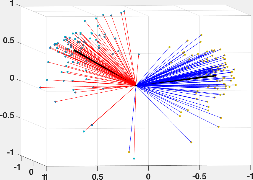
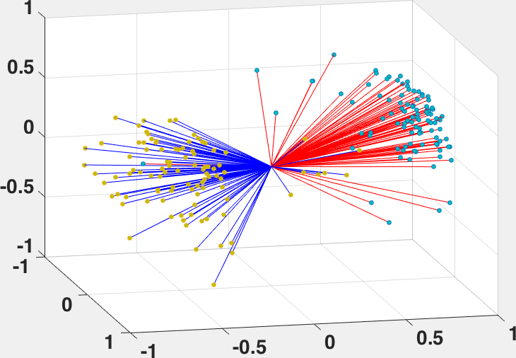
This data set [18] summarises vector-cardiograms of healthy children aged between -. Each child has two vector-cardiograms, using the Frank and McFee system respectively. The two vector-cardiograms are represented as two mutually orthogonal orientations in , hence, each vector-cardiogram can be mapped to a point on . We perform statistical analysis via principal geodesic analysis (PGA) [20] of the data depicted in figure 0(c) (at the top). One of the key steps in PGA is to find the FM, which is depicted in the plot (in black). Further, we reconstructed the data from the first two principal directions (which accounts for of the data variance) and the reconstructed results are shown in the rightmost plot. The reconstruction error is on the average per subject, which implies that the reconstruction is quite accurate.
5.4 Comparison with Stochastic Gradient Descent based FM Estimator
In this subsection, we present a comparison between StiFME and the stochastic gradient descent based FM estimator in [7].
There are two key differences between the algorithm in [7] and StiFME. As in any stochastic gradient scheme, the next point, i.e., in (Eq.2 in [7]) is chosen randomly from the given sample set. Hence, the stochastic formulation needs several passes over the sample set and reports the expected value over the passes as the estimated FM. In contrast, StiFME is a deterministic algorithm and hence does not need multiple passes over the data. Moreover, our selection of this weight is primarily in spirit the same as the weights in a recursive arithmetic mean computation in Euclidean space. In contrast, [7] does not specify any scheme to choose the proper step size (Eq.2 of [7]). Note that, like in any gradient descent, the algorithm in [7] is very much dependent on a proper step size selection. Step size selection in gradient descent and its relatives is a hard problem and the most widely used method (Armijo rule) is computationally expensive. We now provide two experimental comparisons with algorithm in [7]. Consider a data set of samples drawn from a Log-Normal distribution, with a small variance of on . The distance between {FM and StiFME} and {FM and computed FM using the algorithm in [7]} (assessed in one pass over the data) are and respectively. However, [7] requires passes over the data to achieve the tolerance of obtained by StiFME. For a larger data variance of on , the distance between FM, StiFME and FM computed from [7] are and (in one pass over the data) respectively, which is a significant difference. Furthermore, the method in [7] needs passes over the data to achieve the tolerance achieved by StiFME. This clearly indicates better computational efficiency of StiFME over the FM estimator in [7].
5.5 Time Complexity comparison
The complexity of StFME is , is the number of samples in the data and is the number of iterations required for convergence. The number of iterations however depends on the step size used, too small a step size causes very slow convergence and too large a step size overshoots the FM. In contrast, the complexity of StiFME is because it outputs the estimated FM in a single pass through the data. On the other hand the SGD algorithm proposed in [7] takes , where is the batch size and is the number of iterations to convergence. So, in comparison, StiFME is much faster than the other two competing algorithms.
6 Conclusions
In this paper, we defined a Gaussian distribution on a Riemannian homogenous space and proved that the MLE of the location parameter of this Gaussian distribution yields the FM of the samples drawn from the distribution. Further, we presented a sampling algorithm to draw samples from this Gaussian distribution on the Stiefel manifold (which is a homogeneous space) and a novel recursive estimator, StiFME, for computing the FM of these samples. A proof of weak consistency of StiFME was also presented. Further, we also showed that the MLE of the location parameter of the Gaussian distribution on asymptotically achieves the Cramér-Rao lower bound and hence is efficient. The salient feature of StiFME is that it does not require any optimization unlike the traditional methods that seek to optimize the Fréchet functional via gradient descent. This leads to significant savings in computation time and makes it attractive for online applications of FM computation for manifold-valued data, such as clustering etc. We presented several experiments demonstrating the superior performance of StiFME over gradient-descent based competing FM-estimators on synthetic and real data sets.
References
- [1] P-A Absil, Robert Mahony, and Rodolphe Sepulchre. Riemannian geometry of grassmann manifolds with a view on algorithmic computation. Acta Applicandae Mathematicae, 80(2):199–220, 2004.
- [2] Bijan Afsari. Riemannian lp center of mass: Existence, uniqueness, and convexity. Proceedings of the American Mathematical Society, 139(2):655–673, 2011.
- [3] Tsuyoshi Ando, Chi-Kwong Li, and Roy Mathias. Geometric means. Linear algebra and its applications, 385:305–334, 2004.
- [4] Marc Arnaudon, Frédéric Barbaresco, and Le Yang. Riemannian medians and means with applications to radar signal processing. IEEE Journal of Selected Topics in Signal Processing, 7(4):595–604, 2013.
- [5] Rajendra Bhatia. Matrix analysis, volume 169. Springer Science & Business Media, 2013.
- [6] Abhishek Bhattacharya and Rabi Bhattacharya. Statistics on riemannian manifolds: asymptotic distribution and curvature. Proceedings of the American Mathematical Society, 136(8):2959–2967, 2008.
- [7] Silvere Bonnabel. Stochastic gradient descent on riemannian manifolds. Automatic Control, IEEE Transactions on, 58(9):2217–2229, 2013.
- [8] Hasan Ertan Cetingul and René Vidal. Intrinsic mean shift for clustering on stiefel and grassmann manifolds. In Computer Vision and Pattern Recognition, 2009. CVPR 2009. IEEE Conference on, pages 1896–1902. IEEE, 2009.
- [9] Rudrasis Chakraborty, Monami Banerjee, and Baba Vemuri. Statistics on the space of trajectories for longitudinal data analysis. IEEE International Symposium on Biomedical Imaging (Accepted), 2017.
- [10] Rudrasis Chakraborty and Baba C. Vemuri. Recursive frechet mean computation on the grassmannian and its applications to computer vision. In The IEEE International Conference on Computer Vision (ICCV), December 2015.
- [11] Malek Charfi, Zeineb Chebbi, Maher Moakher, and Baba C Vemuri. Bhattacharyya median of symmetric positive-definite matrices and application to the denoising of diffusion-tensor fields. In Biomedical Imaging (ISBI), 2013 IEEE 10th International Symposium on, pages 1227–1230. IEEE, 2013.
- [12] Jeff Cheeger and DG Ebin. Comparison theorems in Riemannian geometry, volume 365. American Mathematical Soc., 1975.
- [13] Guang Cheng and Baba C Vemuri. A novel dynamic system in the space of spd matrices with applications to appearance tracking. SIAM journal on imaging sciences, 6(1):592–615, 2013.
- [14] Yasuko Chikuse. Asymptotic expansions for distributions of the large sample matrix resultant and related statistics on the stiefel manifold. Journal of multivariate analysis, 39(2):270–283, 1991.
- [15] Harald Cramér. Mathematical Methods of Statistics (PMS-9), volume 9. Princeton university press, 2016.
- [16] Navneet Dalal and Bill Triggs. Histograms of oriented gradients for human detection. In CVPR, volume 1, pages 886–893, 2005.
- [17] Gianfranco Doretto, Alessandro Chiuso, Ying Nian Wu, and Stefano Soatto. Dynamic textures. International Journal of Computer Vision, 51(2):91–109, 2003.
- [18] T. Downs, J. Liebman, and W. Mackay. Statistical methods for vectorcardiogram orientations. In Vectorcardiography 2: Proc. XIth International Symp. on Vectorcardiography, 1971.
- [19] P Thomas Fletcher and Sarang Joshi. Riemannian geometry for the statistical analysis of diffusion tensor data. Signal Processing, 87(2):250–262, 2007.
- [20] P Thomas Fletcher, Conglin Lu, Stephen M Pizer, and Sarang Joshi. Principal geodesic analysis for the study of nonlinear statistics of shape. IEEE TMI, 23(8):995–1005, 2004.
- [21] Catherine Fraikin, K Hüper, and P Van Dooren. Optimization over the stiefel manifold. PAMM, 7(1):1062205–1062206, 2007.
- [22] Maurice Fréchet. Les éléments aléatoires de nature quelconque dans un espace distancié. In Annales de l’institut Henri Poincaré, volume 10, pages 215–310. Presses universitaires de France, 1948.
- [23] Colin R Goodall and Kanti V Mardia. Projective shape analysis. Journal of Computational and Graphical Statistics, 8(2):143–168, 1999.
- [24] David Groisser. Newton’s method, zeroes of vector fields, and the riemannian center of mass. Advances in Applied Mathematics, 33(1):95–135, 2004.
- [25] Richard Hartley, Jochen Trumpf, Yuchao Dai, and Hongdong Li. Rotation averaging. IJCV, 103(3):267–305, 2013.
- [26] Soren Hauberg, Aasa Feragen, and Michael J Black. Grassmann averages for scalable robust pca. In Proceedings of the IEEE Conference on Computer Vision and Pattern Recognition, pages 3810–3817, 2014.
- [27] Sigurdur Helgason. Differential geometry, Lie groups, and symmetric spaces, volume 80. Academic press, 1979.
- [28] Harrie Hendriks and Zinoviy Landsman. Mean location and sample mean location on manifolds: asymptotics, tests, confidence regions. Journal of Multivariate Analysis, 67(2):227–243, 1998.
- [29] Jeffrey Ho, Guang Cheng, Hesamoddin Salehian, and Baba Vemuri. Recursive Karcher expectation estimators and geometric law of large numbers. In Proceedings of the Sixteenth International Conference on Artificial Intelligence and Statistics, pages 325–332, 2013.
- [30] Tetsuya Kaneko, Simone Fiori, and Toshihisa Tanaka. Empirical arithmetic averaging over the compact stiefel manifold. Signal Processing, IEEE Transactions on, 61(4):883–894, 2013.
- [31] Hermann Karcher. Riemannian center of mass and mollifier smoothing. Communications on pure and applied mathematics, 30(5):509–541, 1977.
- [32] Wilfrid S Kendall. Probability, convexity, and harmonic maps with small image i: uniqueness and fine existence. Proceedings of the London Mathematical Society, 3(2):371–406, 1990.
- [33] Yui Man Lui. Advances in matrix manifolds for computer vision. Image and Vision Computing, 30(6):380–388, 2012.
- [34] Kanti V Mardia and Peter E Jupp. Directional statistics, volume 494. John Wiley & Sons, 2009.
- [35] Maher Moakher. A differential geometric approach to the geometric mean of symmetric positive-definite matrices. SIMAX, 26(3):735–747, 2005.
- [36] Maher Moakher. On the averaging of symmetric positive-definite tensors. Journal of Elasticity, 82(3):273–296, 2006.
- [37] Vic Patrangenaru and Kanti V Mardia. Affine shape analysis and image analysis. In 22nd Leeds Annual Statistics Research Workshop, 2003.
- [38] Xavier Pennec. Intrinsic statistics on riemannian manifolds: Basic tools for geometric measurements. JMIV, 25(1):127–154, 2006.
- [39] Xavier Pennec, Pierre Fillard, and Nicholas Ayache. A riemannian framework for tensor computing. International Journal of Computer Vision, 66(1):41–66, 2006.
- [40] Duc-Son Pham and Svetha Venkatesh. Robust learning of discriminative projection for multicategory classification on the stiefel manifold. In Computer Vision and Pattern Recognition, 2008. CVPR 2008. IEEE Conference on, pages 1–7. IEEE, 2008.
- [41] C Radakrishna Rao. Differential metrics in probability spaces. Differential geometry in statistical inference, 10:217–240, 1987.
- [42] C Radhakrishna Rao. Information and the accuracy attainable in the estimation of statistical parameters. In Breakthroughs in statistics, pages 235–247. Springer, 1992.
- [43] Salem Said, Lionel Bombrun, Yannick Berthoumieu, and Jonathan Manton. Riemannian gaussian distributions on the space of symmetric positive definite matrices. arXiv preprint arXiv:1507.01760, 2015.
- [44] Salem Said, Hatem Hajri, Lionel Bombrun, and Baba C Vemuri. Gaussian distributions on riemannian symmetric spaces: statistical learning with structured covariance matrices. arXiv preprint arXiv:1607.06929, 2016.
- [45] Hesamoddin Salehian, Rudrasis Chakraborty, Edward Ofori, David Vaillancourt, and Baba C Vemuri. An efficient recursive estimator of the fréchet mean on a hypersphere with applications to medical image analysis. Mathematical Foundations of Computational Anatomy, 2015.
- [46] Christian Schuldt, Ivan Laptev, and Barbara Caputo. Recognizing human actions: a local svm approach. In Pattern Recognition, 2004. ICPR 2004. Proceedings of the 17th International Conference on, volume 3, pages 32–36, 2004.
- [47] Anuj Srivastava, Ian Jermyn, and Shantanu Joshi. Riemannian analysis of probability density functions with applications in vision. In CVPR, pages 1–8, 2007.
- [48] Karl-Theodor Sturm. Probability measures on metric spaces of nonpositive curvature. Contemporary mathematics, 338:357–390, 2003.
- [49] David S Tuch, Timothy G Reese, Mette R Wiegell, and Van J Wedeen. Diffusion mri of complex neural architecture. Neuron, 40(5):885–895, 2003.
- [50] Pavan Turaga, Ashok Veeraraghavan, and Rama Chellappa. Statistical analysis on stiefel and grassmann manifolds with applications in computer vision. In Computer Vision and Pattern Recognition, 2008. CVPR 2008. IEEE Conference on, pages 1–8. IEEE, 2008.
- [51] Yung-Chow Wong. Sectional curvatures of grassmann manifolds. Proceedings of the National Academy of Sciences, 60(1):75–79, 1968.
- [52] Miaomiao Zhang and P Thomas Fletcher. Probabilistic principal geodesic analysis. In Advances in Neural Information Processing Systems, pages 1178–1186, 2013.
- [53] Wolfgang Ziller. Examples of riemannian manifolds with non-negative sectional curvature, 2007.
- [54] Ralf Zimmermann. A matrix-algebraic algorithm for the riemannian logarithm on the stiefel manifold under the canonical metric. SIAM Journal on Matrix Analysis and Applications, 38(2):322–342, 2017.