Strong gravitational lensing by wave dark matter halos

One of the main predictions from Einstein’s General Relativity is the bending of light as it passes close to a massive body. The deflection angle produced by this effect depends on the mass of the deflector, which then acts like a lens. This deflector may be approximated by a point-like mass, like in the case of a star, but for more massive objects like galaxies it is better to represent them as extended masses which are described by their density profiles. For the purposes of this work, we shall consider galactic lenses, and therefore the density profile described in this section will be representing one galaxy acting as a single lens.

The simplest type of lens is a system with a point mass $M$ located close to the line of sight to a luminous source $S$. Due to the gravitational field of the point mass, a light ray is deflected in its path to the observer; this is described by the lens equation in the thin-lens approximation. The same approximation also holds for a mass distribution, in which case the lens equation is [63],

that relates the (unobservable) angle between the line of sight and the path from the observer to the actual position of the source, $\beta$, and to the apparent position of the source (the image), $\theta$, and the mass distribution that is causing the lensing $m(\theta)$.Also, $D_{OL}$ is the angular distance from the observer to the lens, that we denote by the subindex (OL). Here we have assumed that $m(\theta)$ is the projected mass enclosed in a circle of radius $\xi\equiv D_{OL}\theta$; more explicitly, we can write

where $z\equiv\sqrt{r^{2}-\xi^{2}}$ is a coordinate orthogonal to the line of sight, so that $0\leq\xi\leq r$. If the lens system has a finite radius $r_{\rm max}$, then $z_{\rm max}=\sqrt{r^{2}_{\rm max}-\xi}$; otherwise, we can put $z_{\rm max}\to\infty$ in the integral given by Eq. (3b).

Let us consider the case in which the density profile $\rho(r)$ has a characteristic density $\rho_{s}$, and a characteristic radius $r_{s}$, such that $\rho(r)=\rho_{s}f(r/r_{s})$, where $f$ is the function that accounts for the shape of the profile. We can then write Eq. (2) in the dimensionless form

where the different distances are normalized in terms of $r_{s}$: $\beta_{*}=D_{OL}\beta/r_{s}$, $\theta_{*}=D_{OL}\theta/r_{s}$, and then $\xi_{\ast}=\xi/r_{s}=\theta_{\ast}$. The latter equation means that the normalized variables $\xi_{\ast}$ and $\theta_{\ast}$ can be used interchangeably, and then hereafter we will use $\theta_{\ast}$ as our distance variable¹¹ 1 For the sake of simplicity in the notation, we are using the same same angular variables (together with an asterisk) to denote the new normalized distances.. Likewise, the total mass, as given in Eq. (3a), is normalized as

with $z=\sqrt{r^{2}_{\ast}-\theta^{2}_{\ast}}$ and $r_{\ast}=r/r_{s}$. The new parameter $\lambda$ in Eq. (4) is then given by

where we have defined the reduced (dimensionless) angular distances $d_{A}=D_{A}H_{0}/c$. The angular diameter distance $D_{A}$ as a function of redshift is computed in the standard way [39, see e.g.], assuming cosmological model parameters as given by the Planck 2015 results [1]. Equation (6) contains information about the lensing properties of any given model, together with that of the different distances involved in the lens system, namely that between the observer and the lens (OL), the observer and the source (OS), and the lens and the source (LS).²² 2 This is the same parameter used in [31], but also see [72] in which the definition of $\lambda$ differs by a factor of $1/4\pi$.

One particular case of interest is that of perfect alignment between the luminous source and the lens system for which $\beta_{*}(\theta_{*E})=0$. This in turn defines an Einstein ring with radius $R_{E}=D_{OL}\theta_{E}$, and an associated angular radius $\theta_{E}$. In terms of our normalized variables, we see that the normalized angular Einstein radius $\theta_{\ast E}$ directly is the ratio of the Einstein radius to the (characteristic) scale radius of the density profile, $\theta_{\ast E}=R_{E}/r_{s}$. Moreover, the angular radius $\theta_{*E}$ must also be a solution of the equation [see Eq. (4)]

Interestingly enough, Eq. (7) shows that the lensing properties of a system with a density profile of the form $\rho(r)=\rho_{s}f(r/r_{s})$ are independent of the density and distance scales, and are mostly sensitive to the particular shape of the density profile. The physical parameters of the system are then concentrated in the dimensionless parameter $\lambda$ in Eq. (6), and the latter can be calculated from Eq. (7) without any prior knowledge of the given physical scales in the system, namely $\rho_{s}$ and $r_{s}$, under only the assumption of perfect alignment (see Fig. 1 below for an example).

There is a critical value $\lambda_{\rm cr}$ that is the smallest value of $\lambda$ for which an Einstein ring appears, which must correspond to the limit $\theta_{*E}\to 0$ in Eq. (7). As we shall show now, such a critical value can be calculated analytically in the general case. To avoid the divergence at $\theta_{\ast E}=0$ (where $m_{\ast}(0)=0$), we make use of the L’Hôpital rule in Eq. (7), and from Eq. (3a) we finally obtain

where $\Sigma(0)$ is the central value of the projected surface mass density given by Eq. (3b). Eq. (8) is quite a simple formula for the calculation of $\lambda_{\rm cr}$ for any given density profile $\rho(r)$.³³ 3 It should be noted that the definition of $\lambda_{\rm cr}$ depends on the chosen scale radius for normalization $r_{s}$, so that the value obtained from Eq. (8) in our case is considering that $r_{s}$ coincides with the intrinsic distance scale in the density profile $\rho(r)$.

As said before, Eq. (8) suggests that the critical value $\lambda_{\rm cr}$ just depends on the particular shape of the given density profile and no information is necessary about its other physical parameters. The values of $\lambda_{\rm crit}$, calculated from Eq. (8) for density profiles that are well-known in the literature, are shown in Table 1. For these profiles we also show in Fig. 1 the Einstein angle $\theta_{\ast E}$ as calculated from Eq. (7). As expected, the Einstein angle is the smallest for the WaveDM profile (Eq. (10)) alone, which also means that it is the one with the weakest lensing signal.

We should mention here an additional use of Eq. (7) to constrain the free parameters of a given density profile. It relates to the fact that any DM halo characterized by a particular density profile needs to satisfy the constraint $\lambda\geq\lambda_{\rm cr}$ if it is to produce a lensing signal. Using Eqs. (6) and (8), the latter statement can be re-written as

Equation (9) establishes a minimum value for the (structural) surface density $\rho_{s}r_{s}$ of any given DM profile in terms of the measured quantities of a lens system. Although the constraint Eq. (9) is satisfied automatically by the NFW profile, for which $\lambda_{\rm crit}=0$, this is not the case for the other profiles listed in Table 1.

For the density profile of WaveDM halos we will consider the model described in [79, 78], which arises from the study of extensive N-body simulations. The profile consists basically of two parts: one part describing a core sustained by the quantum pressure of the boson particles, also known as the soliton profile, and another part that resembles a NFW-like profile in the outer parts of the halo. As argued in [57], the transition at some radius to a NFW profile must be expected from the change of behavior to CDM on scales larger than the natural length of coherence, which should be proportional to the associated Compton length of the boson particles (in full units, the Compton length is $L_{C}=\hbar/(mc)$, where $\hbar$ is the (reduced) Planck’s constant and $c$ is the speed of light).

The soliton profile is given by

where $r_{s}$ and $\rho_{s}$ are its characteristic radius and central density contrast, respectively. This profile was first studied in detail in [78], although here we are following the nomenclature adopted in [57], where it is also shown that the profile fits well the ground-state solution of the so-called Schrödinger-Poisson (SP) system of equations [75, 37]. In this respect, the soliton profile is strongly related to the wave properties (via the Schrödinger equation) of the boson particles.

One important property of the profile given in Eq. (10) is that it must also obey the intrinsic scaling symmetry of the SP system [37]. If $0<\hat{\lambda}\ll 1$ is a constant parameter, it can be shown that the central density and radius in the soliton profile are given by

This equation suggests that the intrinsic, physical, quantities of the soliton profile in Eq. (10) are related as shown in Eq. (1). This relation will be important later when we discuss the constraints on the boson mass $m_{a}$.

For the NFW profile at the outskirts of the galaxy halo we adopt the following parametrization

Notice that in writing Eq. (12) we are assuming the following implicit definitions for the scale radius and density, respectively, of the NFW profile: $r_{\rm NFW}=r_{s}/\alpha_{\rm NFW}$ and $\rho_{\rm NFW}=\rho_{s}\,\rho_{\rm NFW\ast}$, where both $\alpha_{\rm NFW}$ and $\rho_{\rm NFW\ast}$ are dimensionless numbers.

Unfortunately, there is not precise information in [79] about the transition in a galaxy halo from the soliton profile of Eq. (10) to the NFW profile of Eq. (12) in the general case. Hence, for the present work we adopt the convention for a combined profile as suggested in [57]

where $\Theta(r_{\epsilon}-r)$ is the Heaviside step function. Here, $r_{\epsilon}$ is the matching radius where the transition between the individual profiles occurs, and which satisfies the condition $\rho(r_{\epsilon})=\epsilon\rho_{s}$. Notice that $0<\epsilon<1$ if the transition between the profiles is to occur at the outskirts of the galaxy halo.

In general terms, and under our parametrization, there are six free parameters in the combined profile (Eq. (13)): $(\rho_{s},r_{s},\rho_{\rm NFW\ast},\epsilon,r_{\epsilon},\alpha_{\rm NFW})$. We will now derive two new constraints that arise from the continuity of the combined density profile at the matching radius which will help us to reduce the number of free parameters.

For a continuous density function, we must impose the condition

When Eq. (14) is applied to the soliton profile of Eq. (10), we obtain

Equation (15c) indicates the (normalized) density $\rho_{\rm NFW\ast}$ that is required for a correct matching between the soliton and NFW profiles, for given values of $\alpha_{\rm NFW}$ and $r_{\epsilon\ast}$.

However, one can see that the continuity constraint (Eq. (15c)) actually shows a hidden degeneracy: once the values of $\alpha_{\rm NFW}$ and $\rho_{\rm NFW\ast}$ are fixed, there can be up to two solutions for the matching radius $r_{\epsilon\ast}$. This is a direct consequence of the fact that the crossing of the density profiles (Eqs. (10) and (12)) can occur at most at two different points, as illustrated in the left-hand panel of Fig. 2, which shows normalized density profiles for $\alpha_{NFW}=0.1$ and different values of the normalized density $\rho_{\rm NFW\ast}$.

Fig. 2 (left panel) also shows that there exists a maximum value of $\rho_{\rm NFW\ast}$ beyond which the profiles do not cross each other. This fact can be understood in terms of Eq. (15c), which we evaluate for different values of $\alpha_{\rm NFW}$ in the right-hand panel of Fig. 2. Here we can see that, for each $\alpha_{\rm NFW}$, there is always a maximum value of $\rho_{\rm NFW\ast}$, as a function of the matching radius $r_{\epsilon\ast}$, that corresponds to the case in which the soliton and NFW density profiles barely touch, as seen in the left-hand panel of Fig. 2.

To avoid the hidden degeneracy, and to select always a combined profile with an interior soliton shape, we will choose those cases for which $r_{\epsilon\ast}\geq r_{\rm\epsilon\ast,max}$, where $r_{\rm\epsilon\ast,max}$ is the matching radius corresponding to the maximum value of $\rho_{\rm NFW\ast}$. A straightforward calculation from Eq. (15c) shows that $r_{\rm\epsilon\ast,max}$ is a root of the cubic equation

Although there is a general solution to this equation, it can be shown that the limits for small and large values of $\alpha_{\rm NFW}$ are

This means that in absolute terms the maximum value of $\rho_{\rm NFW\ast}$ must be located in the range $0.25<r_{\rm\epsilon\ast,max}<0.48$, which is in agreement with the values observed in the right-hand panel of Fig. 2. After all this, it is possible to reduce the number of free parameters that describe the combined profile (13) to only four: $\rho_{s}$, $r_{s}$, $r_{\epsilon}$ and $\alpha_{\rm NFW}$. By means of these parameters and the constraints discussed above, the other parameters are fully specified.

Notice that our chosen normalization is such that the physical parameters in the NFW profile (Eq. (12)) are given in terms of those in the soliton profile (Eq. (10)). This means, for instance, that $\rho_{\rm NFW\ast}>1$ ($\rho_{\rm NFW\ast}<1$) is equivalent to $\rho_{\rm NFW}>\rho_{s}$ ($\rho_{\rm NFW}<\rho_{s}$), whatever the physical value of $\rho_{s}$ is. Likewise, we find that $\alpha_{\rm NFW}<1$ ( $\alpha_{\rm NFW}>1$) corresponds to $r_{\rm NFW}>r_{s}$ ($r_{\rm NFW}<r_{s}$), even if the physical value of $r_{s}$ is not known beforehand. The same will apply for the matching radius, since $r_{\epsilon\ast}>1$ ($r_{\epsilon\ast}<1$) means that matching occurs beyond the soliton radius and then $r_{\epsilon}>r_{s}$ (before the soliton radius, and then $r_{\epsilon}<r_{s}$).

It must be noticed also that the prescription above for the matching of the density profiles in Eq. (13) means that the NFW part is always subjected to the presence of the central soliton. For instance, the NFW profile can be diluted away if the matching radius $r_{\epsilon\ast}\to\infty$ (which also means that $\rho_{\rm NFW\ast}\to 0$), and then the density profile becomes the soliton one alone, $\rho(r)\simeq\rho_{\rm sol}(r)$. On the other hand, if $r_{s}\to 0$ the central soliton becomes small but much more massive and more dense, because of the scaling symmetry shown in Eq. (1), so that it dominates the matter contents over that of the NFW profile. The conclusion here is that under our parametrization the density profile (Eq. (13)) can become the soliton profile only if $r_{\epsilon\ast}\to\infty$, but it is not possible to do the same for the NFW part; in this sense, the complete profile (Eq. (13)) should always be seen as that of a central soliton with a subdominant NFW tail.

We want to stress that the complete profile (13) should not be confused with the so-called cored NFW profile that exists already in the literature. The latter is of the form $\rho(r)\sim(r/r_{s})^{-\beta}/(1+r/r_{s})^{2}$ with $0<\beta<1$, and whose lensing properties have been analyzed in [95]. A comparison of the lenses produced by the cored-NFW profile and the WaveDM one is beyond the purpose of this work, as our primary intention is to constrain the parameters in Eq. (13) and to obtain from them credible bounds on the mass of the boson particles.

As a final note, we emphasize the convenience of the chosen parametrization in terms of the soliton characteristic quantities, as the soliton and NFW parameters must follow well defined scaling constraints that are intrinsic to the WaveDM. These scaling properties will then be already explicit in the complete profile (13) when making a comparison of the model with lensing data.

To obtain the lensing properties of the combined profile given by Eq. (13), we follow the recipe described in Sec. II.1. We first need to compute the projected surface mass density (Eq. (3b)). Because of the presence of the step functions in Eq. (13), the integral in Eq. (3b) naturally separates as

It should be understood that the integrals in Eq. (18) are done along the line of sight. Notice also that we are following our convention in Sec. II for normalized quantities, namely $\Sigma_{*}=\Sigma/(\rho_{s}r_{s})$, $\theta_{\ast}=\xi/r_{s}$ and $z=\sqrt{r^{2}_{\ast}-\theta^{2}_{\ast}}$. The analytical expressions for the integrals in Eq. (18) can be found in appendix A.

Equation (18) shows that the projected surface mass density only depends upon the characteristic radii and densities of the combined density profile (Eq. (13)). For instance, if we keep $r_{s}$ fixed, it can be shown that

a result that is obtained from the first branch in Eq. (18). Notice that Eq. (19) is exactly the result for the soliton profile (Eq. (10)) alone. Also, as we have mentioned before, it is not possible to recover the standard result of the surface density for the NFW profile by letting $r_{s}\to 0$, as in this case the matter content is still dominated by the central soliton.

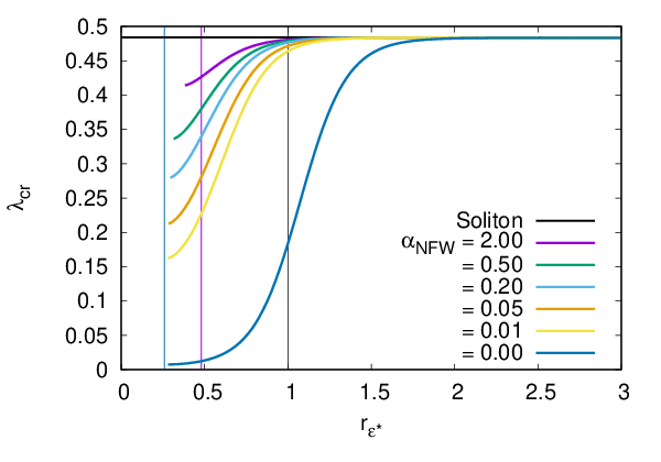
Going back to the complete profile (Eq. (13)), we start with the calculation of the critical value $\lambda_{\rm crit}$ from the analytical formula in Eq. (8). The (total) projected surface mass density for the special value $\theta_{\ast}=0$ is obtained from the first branch, in Eq. (18), as

which indicates, together with Eq. (7), that the critical value $\lambda_{\rm cr}$ of the combined profile (Eq. (13)) is a function of $r_{\epsilon\ast}$ and $\alpha_{\rm NFW}$, and its behavior for different combinations of these parameters is shown in the left panel of Fig. 3. Notice that we have taken into account the constraint $r_{\epsilon\ast}\geq r_{\epsilon\ast,\rm max}$, see Eq. (16). Moreover, it can be seen that the lowest value of $\lambda_{\rm cr}$, for any given value of $\alpha_{\rm NFW}$, is indeed attained at $r_{\epsilon\ast,\rm max}$ as indicated by the vertical lines with the corresponding colors. Not surprisingly, the addition of the NFW outer part helps the soliton profile to achieve small values of $\lambda_{\rm crit}$, which in turn eases the accomplishment of the inequality in Eq. (9). In particular, Fig. 3 shows that $\lambda_{\rm crit}\to 0$ as $\alpha_{\rm NFW}\to 0$, which means that the combined profile (13) will be able to produce a lensing signal for any non-trivial combination of its parameters $\rho_{s}$ and $r_{s}$.

In the case of the combined profile the total mass $M(r)$ inside a sphere of any given radius $r>r_{\epsilon}$ is simply given by the integral

In the general case the total mass diverges as $r\to\infty$, whereas for the soliton profile only (which requires $r_{\epsilon\ast}\to\infty$) we simply obtain that its total mass $M_{s}$ is [37, 57, 22]

In general, we expect from Eq. (20) the total mass in the combined profile to be larger than the soliton alone, that is $M(r)\geq M_{s}$. However, the value of the total mass $M$ will depend on the upper limit of integration $r_{\ast}$, and the largest values for any given $r_{\ast}$ will be obtained for the case where $\alpha_{\rm NFW}\to 0$, similar to the case of the critical value $\lambda_{\rm crit}$. The aforementioned general behaviour of the total mass $M$ as a function of the free parameters $r_{\epsilon\ast}$ and $\alpha_{\rm NFW}$ is shown in the right-hand panel of Fig. 3. For the numerical examples we considered the upper limit of integration $r_{\ast}=20$, for which we then see that that the difference between $M$ and $M_{s}$ can be as large as three orders of magnitude in the case $\alpha_{\rm NFW}=0$. In other words, the total mass in the WaveDM profile is intrinsically attached to that of its soliton, and then the latter should be large enough if we are going to get the right mass scales in galaxies. This is a non-trivial property, as it shows that any non-zero value of the parameter $\alpha_{\rm NFW}$ could point out the existence of a soliton core with a non-negligible mass contribution to the lens system (see for instance Fig. (5) below).

As a first case of study, let us consider the soliton core profile without the external NFW part. There are in this case only two free parameters: $m_{a22}$ and $\theta_{\ast E}$. In section III.2 a Bayesian analysis will be carried out, taking into account the results from this section. The projected mass surface density given by Eq. (5a), with the help of Eq. (19), has in this case an analytical expression,

where $\lambda_{\rm crit}\simeq 0.484$ is the critical value calculated from Eq. (8); see also Table 1. Notice that $m_{\ast}(0)=0$, whereas its asymptotic limit is $m_{\ast}(\infty)=2/(13\lambda_{\rm crit})$.

To obtain a basic understanding of the solutions that will be found for the physical parameters, we show in the left panel of Fig. 4 the expected behavior of the left-hand side of Eq. (22) as a function of the Einstein angle $\theta_{\ast E}$. We also show, as the series of horizontal lines, the values of the right-hand side of Eq. (22) obtained from the observed data for the galaxies listed in Table 2.

Figure 4 shows that it will always be possible to identify a value of the Einstein angle $\theta_{\ast E}$ for which the left-hand and right-hand sides of Eq. (22) are in agreement, irrespective of the value of the boson mass – although as the boson mass increases the agreement occurs at increasingly large values of $\theta_{\ast E}$. For the examples shown in Fig. 4, a boson mass of order $m_{a22}\simeq 0.02$ seems to fit well the SLACS galaxies listed in Table 2 – corresponding to an allowed range for the angular Einstein radius of $5<\theta_{\ast E}<10$. This latter range can also be translated into an allowed range for the soliton radius, and suggests that $r_{s}\sim{\rm kpc}$ for the given example galaxies. However, note that it is always possible to find a solution that matches the left-hand and right-hand side of Eq. (22), for any given value of the boson mass $m_{a}$, by a suitably large choice of Einstein angle $\theta_{\ast E}$, that is, by choosing $r_{s}\to 0$. We must recall that the latter condition means that the density profile is dominated by a very massive and compact soliton, but this can be in disagreement with other indications about the actual size of the dark matter halo in the lens galaxies.

To summarize, given that we have only one observable constraint, the most we can do is first to fix the value of the boson mass $m_{a}$ and from this to obtain constraints on the remaining free parameters that are consistent with that boson mass. Specifically, by adopting a proposed value for the boson mass $m_{a}$ in Eqs. (22) and (23), we can obtain for each galaxy the corresponding best-fit value for $\theta_{\ast E}$, and from that the best-fit value for $r_{s}$.

The results obtained for our selected sample of galaxies are shown in Table 3, and also plotted in the right panel of Fig. 4. The latter figure speaks for itself, and shows that the data points for all galaxies lie along the line with a constant soliton mass $M_{s}\simeq 10^{11}\,M_{\odot}$ (see Eq. (21)), and (as required) all lie below the line that represents the inequality, Eq. (9), for the galaxy in Table 2 (J0935-0003) with the most extreme value for the ratio of distances on the right-hand side of Eq. (22). The different values obtained for the characteristic radius $r_{s}$ give an enclosed mass which corresponds closely to the values reported in [3]. Nevertheless, these models are found to be considerably too compact when the characteristic radius and corresponding enclosed mass are considered together. For example, galaxy J0008-0004 has a value for $M_{\rm Eins}=3.1\times 10^{11}\,M_{\odot}$ which is comparable with the value of $M_{s}=3.4\times 10^{11}\,M_{\odot}$ obtained using the best fit parameters of the soliton model. Notwithstanding that the soliton model gives an enclosed mass that is adequate and realistic, we think that the characteristic radius is most definitely not so. This is by taking into consideration the results from rotation curves where the effects of dark matter are expected to be at larger radii than the luminous part of the galaxy, and this contrasts with the values obtained for the soliton alone where the mean effective radius for galaxy J0008-0004 is observed to be $r_{e}\approx 9.6\,\textrm{kpc}$, which is several orders of magnitude larger than the characteristic radius $r_{s}$ obtained for any of the different boson masses presented in Table 3, including the samples from the other surveys. Therefore we think the soliton profile alone is actually not helping to explain the distribution of dark matter around the selected galaxies in a consistent way.

There are two valuable lessons from the above exercise. The first one is that the soliton core profile alone will always be able to fulfill the lensing constraints even without the consideration of the NFW contribution given the Einstein-radius as the only measurement to satisfy. This is not surprising, as the lensing equations can be solved even if we consider a point particle with the required total mass (which formally corresponds to the soliton core profile with $m_{a}\to\infty$). The second lesson is that even though the soliton profile may be adequate, formally speaking, to explain the lensing properties of the galaxies in Table 2, we will, in any case, have to consider the NFW outskirts in the complete profile (Eq. (13)) in order to satisfy other constraints that suggest that the boson mass should be in the range $m_{a22}=1-10$ [41, see].

Taking into account the above experience gained with the soliton profile alone, we will now consider the following procedure for the complete WaveDM profile. Since the total mass inside the Einstein radius is the only constraint provided by the lens systems, we will fix the values of the boson mass $m_{a}$ and soliton mass $M_{s}$. This approach is considered due to the results from the soliton analysis where the boson mass can satisfy different values for the Einstein radius, and other studies have found that $m_{a}$ needs to be in certain range. For this, we take following values of the boson mass $m_{a22}=0.1,1,10$, and for the soliton mass $\log_{10}(M_{s}/M_{\odot})=11.5,10.5,9.5,8.5,7.5$, from which we will calculate the values of $r_{s}$ by means of Eq. (21), which allows to avoid a possible overcompensation of the soliton mass.

We will adopt a uniform prior for the other parameters over the following ranges: $\alpha_{\rm NFW}=[0:10]$, and $r_{\epsilon\star}=[r_{\epsilon\star,max}:10]$. Here $r_{\epsilon\ast,\rm max}$ is found from the cubic equation (16) for a given value of $\alpha_{\rm NFW}$, and the extreme values $\alpha_{\rm NFW}=10$ and $r_{\epsilon\ast}=10$ are suggested by Figs. 3 and 4.

We will obtain the values of $\theta_{\ast E}$ by sampling from a Gaussian distribution, using the relation

The value for $\theta_{\ast Em}=R_{E}/r_{s}$ is the mean of the distribution using the observed value for the Einstein radius, $\sigma=0.05*\chi$ the error assigned and $p$ is a random number sampled from a uniform distribution on the interval [0,1]. The inverse error function is approximated as described in [93]. In this way, $\theta_{\ast E}$ will not enter into the fitting analysis as an extra variable.

Once the soliton mass is fixed, the rest of the mass that is included within the Einstein radius must be completed by the NFW profile. Because this requires a huge contribution, up to three orders of magnitude more, one sensible consideration is to set the total mass of the lens as composed by a simple representation of luminous matter and the selected model of dark matter. In a first approximation, the mass corresponding to the baryonic matter is simply a constant value modeled as a point particle. This is done from Eq. (2), and then the projected mass for the lens is composed of two parts,

where $m(\theta)$ is the mass from the dark matter component given by the profile in Eq. (13), and $M^{\prime}=f{*,_{Ein}}M_{Ein}$ is the stellar mass contribution as described in Table 2. These values are normalized accordingly and then the dimensionless total mass $m^{\prime}$ is

Eq. (26a) is combined with Eq. (22) to produce a modified observable which uses the soliton mass directly,

Using the samples mentioned in section III we will try to constrain the free parameters that will satisfy Eq. (27). As said before, the information available from the data is the Einstein radius, $R_{E}$, the lens distances ($d_{\rm OL}$, $d_{\rm LS}$, $d_{\rm OS}$), the lens redshift and the source redshift. This information is used in the Multinest code [28] to carry out a parameter search for each individual galaxy. We carried out the analysis on the nine galaxies of our sub-sample of the surveys. Nevertheless, they showed a similar behaviour for the range of values of $f_{*}$.

For brevity only representative results are shown, as in Fig. 5, for the individual cases of galaxies J0935-0003, J0008-0004 and J220329+020518; these cases include the contribution of the luminous matter to the total mass of the lens as in Eq. (27). For the purposes of clarity, in each figure we indicate the radius $r_{s}$ and total mass $M_{s}$ of the soliton profile. We note that the free parameters $r_{\epsilon\ast}$ and $\alpha_{\rm NFW}$ appear well constrained if the soliton mass cannot provide the total mass required by the lens system; in the examples shown, this happens if $M_{s}<10^{11.5}\,M_{\odot}$. Secondly, the credible regions for the parameters in Fig. 5 are in agreement with the theoretical expectations discussed in Sec. II.2: there is a minimum value for $r_{\epsilon\ast}$ due to the constraint imposed by Eq. (16), and a maximum value of $\alpha_{\rm NFW}$ appears due to the maximal contribution of the NFW part of the profile to the total mass in the lens, see also the right panel in Fig. 3. Likewise, notice that as $\alpha_{\rm NFW}\to 0$ the value of the matching radius $r_{\epsilon\ast}$ is very well constrained, and this is easily understood from Eq. (20): it is $r_{\epsilon\ast}$ which determines alone the contribution of the NFW part of the profile to the total mass. Indeed, according to our parametrization in Sec. II.2 the NFW part of the density profile, under the limit $\alpha_{\rm NFW}\to 0$, becomes

Apart from the presence of $r_{\epsilon\ast}$ (which in this case is bounded from above $r_{\epsilon\ast}\leq 1/\sqrt{15}$, see Eq. (17a)), we also see that the behavior $1/r$ is the only one that survives from the NFW functional form, and then our results indicate that the outermost behavior $1/r^{3}$ is left unconstrained.

Finally, observe that the value $\log_{10}(M_{s}/M_{\odot})=7.5$ is excluded because the soliton mass $M_{s}$ is so small that the NFW part cannot compensate the required mass for the lens. Recall that there is a matching (continuity) condition for the density profile in which the NFW density $\rho_{NFW}$ is always smaller than $\rho_{s}$, and this condition makes the NFW part of the profile unable to account for the total mass of the lens even in the limit $\alpha_{\rm NFW}\to 0$.

In summary, if the soliton is allowed to provide enough mass to fulfill the matter contribution in the lens, say $M_{s}\sim 10^{11.5}\,M_{\odot}$, the analysis will select large values for $r_{\epsilon\ast}$ so that the NFW tail contribution to the total matter is minimal, see Eq. (20). In contrast, if the soliton mass is not large enough, $M_{s}<10^{11.5}\,M_{\odot}$, it is then possible to find appropriate pairs $(\alpha_{\rm NFW},r_{\epsilon\ast})$ for the NFW part of the profile to provide the needed mass for the lens. In this respect, the striped credible regions in Fig. 5 represent the degeneracy regions in the plane $(\alpha_{\rm NFW},r_{\epsilon\ast})$ for the same mass contribution of the NFW tail to the lens system. Thus, we can see that distinct credible regions can be found for the NFW parameters if the soliton mass is $10^{8.5}<M_{s}/M_{\odot}<10^{11.5}$, and that the constraints are in agreement with the semi-analytic analysis in Sec. II.

Another quantity of interest is the resultant density profile of DM in the lens system. Fig. 6 shows examples of the density profiles inferred from the posteriors of galaxy J0008-0004 in Fig. 5 for a boson mass $m_{a22}=1$. The soliton core is clearly seen in all curves, and so too is the transition to the NFW part of the profile. The corresponding matching radius $r_{\epsilon}$, in full units, is selected to be at $15.36$ pc, $19.34$ pc, $96.94$ pc and $969.4$ pc for the soliton masses $10^{11.5}M_{\odot}$, $10^{10.5}M_{\odot}$, $10^{9.5}M_{\odot}$ and $10^{8.5}M_{\odot}$, respectively. Not surprisingly, the largest core corresponds to the configuration with the lowest soliton mass for which the matching radius is close to the lower bound suggested in Eq. (17a).

We also report in Fig. 7 the results obtained for the lens system J0008-0004 and J220329+020518, for larger or smaller values of the boson mass. For the boson mass $m_{a22}=10$ we obtain good constraints on the NFW parameters, but the soliton core is very compact in all cases, although a constraint cannot be found if $M_{s}=10^{6.5}\,M_{\odot}$. For the boson mass of $m_{a22}=0.1$, we can only obtain well defined constraints on the NFW parameters when the soliton mass is $M_{s}=10^{10.5}\,M_{\odot}$, but not for larger or smaller values. Low values of $M_{s}$ imply values of the soliton radius $r_{s}$ that are larger than the Einstein radius, and this kind of cases are unable to satisfy the lensing constraints. Hence, for a mass of $m_{a22}=10$, the soliton is much more compact, and it is not by itself adequate to describe a galaxy. But given the fact that the parameters $\alpha_{\rm NFW}$ and $r_{\epsilon\ast}$ are also well constrained we conclude that the lensing effect must be mostly attributed to the NFW part. This is not surprising, as we had already indicated in Sec. II.3 that strong lensing could be achieved if $\alpha_{\rm NFW}\ll 1$. Moreover, a larger boson mass is also in better agreement with recent cosmological constraints [42, see] and with estimations based upon satellite galaxies of the Milky Way and Andromeda [91, see].

In contrast, we can see that the constraints become more diffuse if we consider a smaller boson mass of $m_{a22}=0.1$, although there seems to be some preference for the case in which $M_{s}=10^{10.5}$, that also corresponds to a larger soliton radius. This time the resultant configuration would be in agreement with those found in the statistical analysis carried out in [33], which suggests that satellite galaxies put an upper bound on the boson mass that takes the form $m_{a22}<0.4$.

References

- [1] Ade, P. A. R., et al. 2016, Astron. Astrophys., 594, A13
- [2] Armengaud, E., Palanque-Delabrouille, N., Marsh, D. J. E., Baur, J., & Yèche, C. 2017, arXiv:1703.09126
- [3] Auger, M. W., Treu, T., Bolton, A. S., et al. 2009, ApJ, 705, 1099
- [4] —. 2010, ApJ, 724, 511–525
- [5] Bartelmann, M. 1996, A&A, 313, 697–702
- [6] Bernal, T., Fernández-Hernández, L. M., Matos, T., & Rodríguez-Meza, M. A. 2017, arXiv:1701.00912
- [7] Biesiada, M., Piórkowska, A., & Malec, B. 2010, Monthly Notices of the Royal Astronomical Society, 406, 1055–1059. http://dx.doi.org/10.1111/j.1365-2966.2010.16725.x
- [8] Böhmer, C. G., & Harko, T. 2007, J. Cosmology Astropart. Phys, 6, 025
- [9] Bolton, A. S., Burles, S., Koopmans, L. V. E., et al. 2008a, ApJ, 682, 964–984
- [10] Bolton, A. S., Burles, S., Koopmans, L. V. E., Treu, T., & Moustakas, L. A. 2006, ApJ, 638, 703–724
- [11] Bolton, A. S., Treu, T., Koopmans, L. V. E., et al. 2008b, ApJ, 684, 248–259
- [12] Boylan-Kolchin, M., Bullock, J. S., & Kaplinghat, M. 2011, mnras, 415, L40
- [13] Bullock, J. S., & Boylan-Kolchin, M. 2017, Ann. Rev. Astron. Astrophys., 55, 343
- [14] Burkert, A. 1995, The Astrophysical Journal Letters, 447, L25. http://stacks.iop.org/1538-4357/447/i=1/a=L25
- [15] Cao, S., Biesiada, M., Gavazzi, R., Piórkowska, A., & Zhu, Z.-H. 2015, The Astrophysical Journal, 806, 185. http://stacks.iop.org/0004-637X/806/i=2/a=185
- [16] Cao, S., Biesiada, M., Yao, M., & Zhu, Z.-H. 2016, Mon. Not. Roy. Astron. Soc., 461, 2192–2199
- [17] Cao, S., Covone, G., & Zhu, Z.-H. 2012, ApJ, 755, 31
- [18] Cao, S., Li, X., Biesiada, M., et al. 2017, The Astrophysical Journal, 835, 92. http://stacks.iop.org/0004-637X/835/i=1/a=92
- [19] Cao, S., & Zhu, Z.-H. 2012, Astron. Astrophys., 538, A43
- [20] Cardone, V. F. 2004, A&A, 415, 839–848
- [21] Cardone, V. F., Tortora, C., Molinaro, R., & Salzano, V. 2009, A&A, 504, 769
- [22] Chen, S.-R., Schive, H.-Y., & Chiueh, T. 2016, arXiv:1606.09030
- [23] Collett, T. E., Oldham, L. J., Smith, R. J., et al. 2018, Science, 360, 1342. http://science.sciencemag.org/content/360/6395/1342
- [24] Cyr-Racine, F.-Y., Sigurdson, K., Zavala, J., et al. 2016, Phys. Rev., D93, 123527
- [25] de Blok, W. J. G. 2010, Advances in Astronomy, 2010, 14 pages
- [26] Diez-Tejedor, A., Gonzalez-Morales, A. X., & Profumo, S. 2014, Phys. Rev., D90, 043517
- [27] Drewes, M., et al. 2017, JCAP, 1701, 025
- [28] Feroz, F., Hobson, M. P., & Bridges, M. 2009, Mon. Not. Roy. Astron. Soc., 398, 1601
- [29] Futamase, T., & Yoshida, S. 2001, Progress of Theoretical Physics, 105, 887–891
- [30] Gavazzi, R., Treu, T., Rhodes, J. D., et al. 2007, ApJ, 667, 176
- [31] González-Morales, A. X., Diez-Tejedor, A., Ureña-López, L. A., & Valenzuela, O. 2013, Phys. Rev. D, 87, 021301
- [32] Gonzalez-Morales, A. X., Diez-Tejedor, A., Urena-Lopez, L. A., & Valenzuela, O. 2013, Phys. Rev., D87, 021301
- [33] González-Morales, A. X., Marsh, D. J. E., Peñarrubia, J., & Ureña-López, L. 2016, arXiv:1609.05856
- [34] Gonzalez-Samaniego, A., Avila-Reese, V., & Colin, P. 2016, Astrophys. J., 819, 101
- [35] Goodman, J. 2000, New A, 5, 103
- [36] Grillo, C., Lombardi, M., & Bertin, G. 2008, A&A, 477, 397–406
- [37] Guzman, F. S., & Urena-Lopez, L. A. 2004, Phys. Rev., D69, 124033
- [38] Hlozek, R., Grin, D., Marsh, D. J. E., & Ferreira, P. G. 2015, Phys. Rev., D91, 103512
- [39] Hogg, D. W. 1999, ArXiv Astrophysics e-prints, astro-ph/9905116
- [40] Hu, W., Barkana, R., & Gruzinov, A. 2000, Physical Review Letters, 85, 1158
- [41] Hui, L., Ostriker, J. P., Tremaine, S., & Witten, E. 2017, Phys. Rev. D, 95, 043541. https://link.aps.org/doi/10.1103/PhysRevD.95.043541
- [42] Iršič, V., Viel, M., Haehnelt, M. G., Bolton, J. S., & Becker, G. D. 2017, arXiv:1703.04683
- [43] Jie, A., Bao-Rong, C., & Li-Xin, X. 2016, Chinese Physics Letters, 33, 079801
- [44] Kaplinghat, M., Tulin, S., & Yu, H.-B. 2016, Phys. Rev. Lett., 116, 041302
- [45] Keeton, C. R. 2001, ArXiv Astrophysics e-prints, astro-ph/0102341
- [46] Klypin, A. A., Kravtsov, A. V., Valenzuela, O., & Prada, F. 1999, Astrophys. J., 522, 82
- [47] Kochanek, C. S. 1991, ApJ, 373, 354
- [48] Kochanek, C. S., Keeton, C. R., & McLeod, B. A. 2001, ApJ, 547, 50
- [49] Koopmans, L. V. E. 2005, MNRAS, 363, 1136–1144
- [50] Koopmans, L. V. E., Treu, T., Bolton, A. S., Burles, S., & Moustakas, L. A. 2006, ApJ, 649, 599–615
- [51] Lee, J.-W. 2017a, ArXiv e-prints, arXiv:1704.05057
- [52] —. 2017b, ArXiv e-prints, arXiv:1704.05057
- [53] Linares Cedeño, F. X., Gonzalez-Morales, A. X., & Arturo Ureña-López, L. 2017, arXiv:1703.10180
- [54] Lyskova, N., Churazov, E., & Naab, T. 2018, MNRAS, 475, 2403
- [55] Maccio, A. V., Paduroiu, S., Anderhalden, D., Schneider, A., & Moore, B. 2012, Mon. Not. Roy. Astron. Soc., 424, 1105
- [56] Marsh, D. J. E., & Pop, A.-R. 2015, Mon. Not. Roy. Astron. Soc., 451, 2479
- [57] Marsh, D. J. E., & Pop, A.-R. 2015, ArXiv e-prints, arXiv:1502.03456
- [58] Matos, T., Guzman, F. S., & Urena-Lopez, L. A. 2000, Class.Quant.Grav., 17, 1707
- [59] Matos, T., & Urena-Lopez, L. A. 2001, Phys.Rev., D63, 063506
- [60] Mitchell, J. L., Keeton, C. R., Frieman, J. A., & Sheth, R. K. 2005, ApJ, 622, 81–98
- [61] Mocz, P., Vogelsberger, M., Robles, V., et al. 2017, arXiv:1705.05845
- [62] Mollerach, S., & Roulet, E. 2002, Gravitational Lensing and Microlensing (World Scientific). https://books.google.co.uk/books?id=vaN2ngEACAAJ
- [63] Mollerach, S., & Roulet, E. 2002, Gravitational Lensing and Microlensing, doi:10.1142/4890
- [64] Muñoz, J. A., Kochanek, C. S., & Keeton, C. R. 2001, The Astrophysical Journal, 558, 657. http://stacks.iop.org/0004-637X/558/i=2/a=657
- [65] Nair, S., & Garrett, M. A. 1996, in Astrophysical Applications of Gravitational Lensing, ed. C. S. Kochanek & J. N. Hewitt (Dordrecht: Springer Netherlands), 195–196
- [66] Navarro, J. F., Frenk, C. S., & White, S. D. M. 1997, ApJ, 490, 493
- [67] Newton, E. R., Marshall, P. J., Treu, T., et al. 2011, ApJ, 734, 104
- [68] Niikura, H., Takada, M., Okabe, N., Martino, R., & Takahashi, R. 2015, PASJ, 67, 103
- [69] Ofek, E. O., Maoz, D., Rix, H.-W., Kochanek, C. S., & Falco, E. E. 2006, The Astrophysical Journal, 641, 70. http://stacks.iop.org/0004-637X/641/i=1/a=70
- [70] Ofek, E. O., Rix, H.-W., & Maoz, D. 2003, Monthly Notices of the Royal Astronomical Society, 343, 639–652. http://dx.doi.org/10.1046/j.1365-8711.2003.06707.x
- [71] Oh, S.-H., de Blok, W. J. G., Brinks, E., Walter, F., & Kennicutt, J. R. C. 2011, aj, 141, 193
- [72] Park, Y., & Ferguson, H. C. 2003, apjl, 589, L65
- [73] Planck Collaboration, Ade, P. A. R., Aghanim, N., et al. 2015, ArXiv e-prints, arXiv:1502.01589
- [74] Robles, V. H., & Matos, T. 2013, Phys. Rev. D, 88, 083008
- [75] Ruffini, R., & Bonazzola, S. 1969, Phys. Rev., 187, 1767
- [76] Sawala, T., Guo, Q., Scannapieco, C., Jenkins, A., & White, S. 2011, MNRAS, 413, 659
- [77] Schive, H.-Y., & Chiueh, T. 2017, arXiv:1706.03723
- [78] Schive, H.-Y., Liao, M.-H., Woo, T.-P., et al. 2014, Physical Review Letters, 113, 261302
- [79] Schive Hsi-Yu, Chiueh Tzihong, & Broadhurst Tom. 2014, Nat Phys, 10, 496. http://www.nature.com/nphys/journal/v10/n7/abs/nphys2996.html#supplementary-information
- [80] Schneider, P., Ehlers, J., & Falco, E. 1999, Gravitational Lenses, Astronomy and Astrophysics Library (Springer). https://books.google.co.uk/books?id=sPAIgy9QGBsC
- [81] Schwabe, B., Niemeyer, J. C., & Engels, J. F. 2016, Phys. Rev., D94, 043513
- [82] Sereno, M. 2002, A&A, 393, 757–764
- [83] Sonnenfeld, A., Gavazzi, R., Suyu, S. H., Treu, T., & Marshall, P. J. 2013a, The Astrophysical Journal, 777, 97. http://stacks.iop.org/0004-637X/777/i=2/a=97
- [84] Sonnenfeld, A., Treu, T., Gavazzi, R., et al. 2013b, The Astrophysical Journal, 777, 98. http://stacks.iop.org/0004-637X/777/i=2/a=98
- [85] Suárez, A., Robles, V. H., & Matos, T. 2014, in Astrophysics and Space Science Proceedings, Vol. 38, Accelerated Cosmic Expansion, ed. C. Moreno González, J. E. Madriz Aguilar, & L. M. Reyes Barrera, 107
- [86] Suyu, S. H., Treu, T., Hilbert, S., et al. 2014, The Astrophysical Journal Letters, 788, L35. http://stacks.iop.org/2041-8205/788/i=2/a=L35
- [87] Tortora, C., Napolitano, N. R., Roy, N., et al. 2018, MNRAS, 473, 969
- [88] Treu, T., & Koopmans, L. V. E. 2004, The Astrophysical Journal, 611, 739. http://stacks.iop.org/0004-637X/611/i=2/a=739
- [89] Trick, W. H., van de Ven, G., & Dutton, A. A. 2016, MNRAS, 463, 3151
- [90] Ureña-López, L. A., & Gonzalez-Morales, A. X. 2016, JCAP, 1607, 048
- [91] Ureña-López, L. A., Robles, V. H., & Matos, T. 2017, arXiv:1702.05103
- [92] Veltmaat, J., & Niemeyer, J. C. 2016, Phys. Rev., D94, 123523
- [93] Winitzki, S. 2008, A handy approximation for the error function and its inverse, , . {http://sites.google.com/site/winitzki/sergei-winitzkis-files/erf-approx.pdf}
- [94] Wright, C. O., & Brainerd, T. G. 2000, apj, 534, 34
- [95] Wyithe, J. S. B., Turner, E. L., & Spergel, D. N. 2001, The Astrophysical Journal, 555, 504. http://stacks.iop.org/0004-637X/555/i=1/a=504
- [96] Zhang, U.-H., & Chiueh, T. 2017a, arXiv:1705.01439
- [97] —. 2017b, Phys. Rev., D96, 023507