跳到论文正文
W Papers独立论文阅读器 arXiv:1707.09833 论文正文 计算阅读时间 · 0%
引用这篇论文根据当前论文元数据生成,正式投稿前建议核对。


License: arXiv.org perpetual non-exclusive license
arXiv:1707.09833v2 [math.PR] 16 Apr 2019

Random gluing of metric spaces

Delphin Sénizergues
Abstract

We construct random metric spaces by gluing together an infinite sequence of pointed metric spaces that we call blocks. At each step, we glue the next block to the structure constructed so far by randomly choosing a point on the structure and then identifying it with the distinguished point of the block. The random object that we study is the completion of the structure that we obtain after an infinite number of steps. In [7], Curien and Haas study the case of segments, where the sequence of lengths is deterministic and typically behaves like n−αn^{-\alpha}. They proved that for α>0\alpha>0, the resulting tree is compact and that the Hausdorff dimension of its set of leaves is α−1\alpha^{-1}. The aim of this paper is to handle a much more general case in which the blocks are i.i.d. copies of the same random metric space, scaled by deterministic factors that we call (λn)n≥1(\lambda_{n})_{n\geq 1}. We work under some conditions on the distribution of the blocks ensuring that their Hausdorff dimension is almost surely dd, for some d≥0d\geq 0. We also introduce a sequence (wn)n≥1(w_{n})_{n\geq 1} that we call the weights of the blocks. At each step, the probability that the next block is glued onto any of the preceding blocks is proportional to its weight. The main contribution of this paper is the computation of the Hausdorff dimension of the set ℒ\mathcal{L} of points which appear during the completion procedure when the sequences (λn)n≥1(\lambda_{n})_{n\geq 1} and (wn)n≥1(w_{n})_{n\geq 1} typically behave like a power of nn, say n−αn^{-\alpha} for the scaling factors and n−βn^{-\beta} for the weights, with α>0\alpha>0 and β∈ℝ\beta\in\mathbb{R}. For a large domain of α\alpha and β\beta we have the same behaviour as the one observed in [7], which is that dimH​(ℒ)=α−1\mathrm{dim_{H}}(\mathcal{L})=\alpha^{-1}. However for β>1\beta>1 and α<1/d\alpha<1/d, our results reveal an interesting phenomenon: the dimension has a non-trivial dependence in α\alpha, β\beta and dd, namely

dimH​(ℒ)=2​β−1−2​(β−1)​(β−α​d)α.\displaystyle\mathrm{dim_{H}}(\mathcal{L})=\frac{2\beta-1-2\sqrt{(\beta-1)(\beta-\alpha d)}}{\alpha}.

The computation of the dimension in the latter case involves new tools, which are specific to our model.

Refer to caption
Figure 1: Gluing of circles of radii λn=n−3/5\lambda_{n}=n^{-3/5}, with weights wn=n−3/2w_{n}=n^{-3/2}. The Hausdorff dimension of the resulting metric space is (103−5)(\frac{10}{3}-\sqrt{5}).

1 Introduction

Let us recall Aldous’ famous line-breaking construction of the Brownian CRT (Continuum Random Tree) in [3]. On the half-line [0,∞)\mathopen{[}0\mathclose{}\mathpunct{},\infty\mathclose{)}, consider C1,C2,…,CnC_{1},\ C_{2},\dots,C_{n} the points of a Poisson process with intensity t​d​tt\mathrm{d}t. Cut the half-line in closed intervals [Ci,Ci+1]\mathopen{[}C_{i}\mathclose{}\mathpunct{},C_{i+1}\mathclose{]}, which we call branches (of length Ci+1−CiC_{i+1}-C_{i}). Starting from [0,C1]\mathopen{[}0\mathclose{}\mathpunct{},C_{1}\mathclose{]}, construct a tree by recursively gluing the branch [Ci,Ci+1]\mathopen{[}C_{i}\mathclose{}\mathpunct{},C_{i+1}\mathclose{]} to a random point chosen uniformly on the tree already constructed (i.e. under the normalised length measure). Aldous’ Brownian CRT is the completion of the tree constructed after an infinite number of steps. This process can be generalised by using any arbitrary sequence (λn)(\lambda_{n}) for the length of the successive branches. This model was introduced and studied by Curien and Haas in [7], who proved that when λn=n−α+o(1)\lambda_{n}=n^{-\alpha+o\mathopen{}\left(1\right)} for some α>0\alpha>0, the tree obtained is a.s. compact and has Hausdorff dimension (1∨α−1)(1\vee\alpha^{-1}). In [4], Amini et. al. obtained a necessary and sufficient condition on the sequence (λn)(\lambda_{n}) for the almost sure compactness of the resulting tree, under the assumption that this sequence is non-increasing. In [13], Haas describes how the height of the tree explodes when n→∞n\rightarrow\infty under the assumption that λn≈nα\lambda_{n}\approx n^{\alpha}, with α≥0\alpha\geq 0.

Our goal is to define a more general version of this model, in which the branches are replaced by arbitrary (and possibly random) measured metric spaces, and to investigate the compactness and the Hausdorff dimension of the resulting metric space. As we will see, in this broader context, a striking phenomenon (absent from [7]) pops up. In all the paper we will work with

(λn)n≥1and(wn)n≥1,(\lambda_{n})_{n\geq 1}\quad\text{and}\quad(w_{n})_{n\geq 1},

two sequences of non-negative real numbers that will be the scaling factors and weights of the metric spaces that we glue. All the scaling factors (λn)n≥1(\lambda_{n})_{n\geq 1} are considered strictly positive, but the weights, except for the first one w1w_{1}, can possibly be null.

Definition of the model and main results

Let us first present a simpler version of our construction, in which we construct a tree through an aggregation of segments. For now the branches, which we denote (𝐛n)n≥1(\mathbf{b}_{n})_{n\geq 1}, are segments of length (λn)n≥1(\lambda_{n})_{n\geq 1}, rooted at one end and endowed with the Lebesgue measure normalised so that their respective total measure is (wn)n≥1(w_{n})_{n\geq 1} (or endowed with the null measure for branches with vanishing weight). We then define a sequence (𝒯n)n≥1(\mathcal{T}_{n})_{n\geq 1} of increasing trees by gluing those branches as follows. First, 𝒯1=𝐛1\mathcal{T}_{1}=\mathbf{b}_{1}. Then, if 𝒯n\mathcal{T}_{n} is constructed, we build 𝒯n+1\mathcal{T}_{n+1} by first sampling a point XnX_{n} chosen proportionally to the measure μn\mu_{n} obtained by aggregating the measures concentrated on the branches 𝐛1,…,𝐛n\mathbf{b}_{1},\dots,\mathbf{b}_{n} and then gluing 𝐛n+1\mathbf{b}_{n+1} onto 𝒯n\mathcal{T}_{n} by identifying its root with XnX_{n}. Let 𝒯∗\mathcal{T}^{*} be the increasing union of the trees 𝒯n\mathcal{T}_{n} for n≥1n\geq 1 and 𝒯\mathcal{T} be the completion of 𝒯∗\mathcal{T}^{*}. Note that if (wn)=(λn)(w_{n})=(\lambda_{n}), this model coincides with the one studied in [7].

We can compute the Hausdorff dimension of the resulting tree in the case where (λn)(\lambda_{n}) and (wn)(w_{n}) behave like powers of nn, say λn=n−α\lambda_{n}=n^{-\alpha} and wn=n−βw_{n}=n^{-\beta}. We define ℒ:=(𝒯∖𝒯∗)\mathcal{L}:=(\mathcal{T}\setminus\mathcal{T}^{*}) to which we refer as the set of leaves of 𝒯\mathcal{T}. In this particular case it coincides, up to a countable set, with the set of points xx such that 𝒯∖{x}\mathcal{T}\setminus\{x\} remains connected. In the above context a trivial consequence of our main theorem is that 𝒯\mathcal{T} is a.s. compact and

dimH​(ℒ)\displaystyle\mathrm{dim_{H}}(\mathcal{L}) =2​β−1−2​(β−1)​(β−α)αif β>1 and α<1,\displaystyle=\frac{2\beta-1-2\sqrt{(\beta-1)(\beta-\alpha)}}{\alpha}\quad\text{if }\beta>1\text{ and }\alpha<1,
=1αotherwise,\displaystyle=\frac{1}{\alpha}\quad\text{otherwise,}

where dimH​(X)\mathrm{dim_{H}}(X) stands for the Hausdorff dimension of the metric space XX, see Section A.2.

Note that, since we can check that the dimension of the skeleton 𝒯∗\mathcal{T}^{*} is always 11, we can recover the dimension of 𝒯\mathcal{T} as dimH​(𝒯)=max⁡(1,dimH​(ℒ))\mathrm{dim_{H}}(\mathcal{T})=\max(1,\mathrm{dim_{H}}(\mathcal{L})). We see that dimH​(ℒ)=1α\mathrm{dim_{H}}(\mathcal{L})=\frac{1}{\alpha} as in [7] for most values of β\beta, however, a new phenomenon, absent from [7], happens in the case β>1\beta>1 (the sum of the weights is finite) and α<1\alpha<1 (the total length is infinite). In this case, the Hausdorff dimension of 𝒯\mathcal{T} depends in a non-trivial manner on α\alpha and β\beta.

Now we want to generalise it to sequences (𝐛n)(\mathbf{b}_{n}) of more general metric spaces that we call blocks, which can be random and possibly more elaborate than just segments. Specifically, our blocks are based on the distribution of a random pointed measured compact metric space, (𝖡,𝖣,ρ,ν)(\mathsf{B},\mathsf{D},\rho,\nu), with underlying set 𝖡\mathsf{B}, distance 𝖣\mathsf{D}, distinguished point ρ\rho and endowed with a probability measure ν\nu. We sometimes denote it 𝖡\mathsf{B} by abuse of notation when no confusion is possible and we refer to it as the underlying random block. We consider a sequence ((,,,,,,,))n≥1\left((\mathsf{B}_{n},\mathsf{D}_{n},\rho_{n},\nu_{n})\right)_{n\geq 1} of i.i.d. random variables with the distribution of (𝖡,𝖣,ρ,ν)(\mathsf{B},\mathsf{D},\rho,\nu) and define our blocks by setting

∀n≥1,(𝐛n,𝐝n,𝝆n,𝝂n):=(𝖡n,λn⋅𝖣n,ρn,wn⋅νn),\forall n\geq 1,\quad(\mathbf{b}_{n},\mathbf{d}_{n},\boldsymbol{\rho}_{n},\boldsymbol{\nu}_{n}):=(\mathsf{B}_{n},\lambda_{n}\cdot\mathsf{D}_{n},\rho_{n},w_{n}\cdot\nu_{n}), (1)

meaning that we dilate all the distances in the space 𝖡n\mathsf{B}_{n} by the factor λn\lambda_{n} and scale the measure by wnw_{n}. We suppose that, λn≈n−α\lambda_{n}\approx n^{-\alpha} for some α>0\alpha>0, and wn≈n−βw_{n}\approx n^{-\beta} for some β∈ℝ\beta\in\mathbb{R}, in some loose sense which we make precise in the sequel. For technical reasons, we have to separate the case β<1\beta<1, the case β>1\beta>1 and β=1\beta=1. This gives rise to the three hypotheses Hyp. ○ α , β , Hyp. ⋄ α , β and Hyp. □ α , 1 . For any d∈[0,∞)d\in\mathopen{[}0\mathclose{}\mathpunct{},\infty\mathclose{)}, we will introduce the Hypothesis H d and suppose that the distribution of our underlying random block (𝖡,𝖣,ρ,ν)(\mathsf{B},\mathsf{D},\rho,\nu) satisfies this hypothesis for some d≥0d\geq 0. This hypothesis ensures that our random block exhibits a dd-dimensional behaviour. We set out all these hypotheses just below the statement of our theorem.

Except in Section 2.1, we will always assume that the blocks are of the form (1). This is implicit in all our results.

In this extended setting, we can perform the same gluing algorithm and build a sequence (𝒯n)n≥1(\mathcal{T}_{n})_{n\geq 1} of random compact metric spaces by iteratively gluing the root of 𝐛n+1\mathbf{b}_{n+1} onto a point chosen in 𝒯n\mathcal{T}_{n} according to the measure μn\mu_{n} obtained as the sum of the measures of the blocks 𝐛1,…,𝐛n\mathbf{b}_{1},\dots,\mathbf{b}_{n}. Again 𝒯∗=⋃n≥1𝒯n\mathcal{T}^{*}=\bigcup_{n\geq 1}\mathcal{T}_{n} is called the skeleton of the construction and its completion is still denoted 𝒯\mathcal{T}. See Figure 1 for non-isometric, non-proper representation in the plane of a simulation of this model, with 𝖡\mathsf{B} chosen to be almost surely a circle of unit length. As for the case of segments, we refer to ℒ=(𝒯∖𝒯∗)\mathcal{L}=\left(\mathcal{T}\setminus\mathcal{T}^{*}\right) as the set of leaves of the construction. We can now state our main theorem.

Theorem 1.
Suppose that there exists d≥0d\geq 0, such that (𝖡,𝖣,ρ,ν)(\mathsf{B},\mathsf{D},\rho,\nu) satisfies Hypothesis H d , and α>0\alpha>0 and β∈ℝ\beta\in\mathbb{R} such that the sequences (wn)(w_{n}) and (λn)(\lambda_{n}) satisfy either Hyp. ⋄ α , β or Hyp. ○ α , β , or Hyp. □ α , 1 . Then, almost surely, the structure 𝒯\mathcal{T} resulting from the construction is compact, and

dimH​(ℒ)\displaystyle\mathrm{dim_{H}}(\mathcal{L}) =2​β−1−2​(β−1)​(β−α​d)α,if β>1 and α<1d,\displaystyle=\frac{2\beta-1-2\sqrt{(\beta-1)(\beta-\alpha d)}}{\alpha},\quad\text{if }\beta>1\text{ and }\alpha<\frac{1}{d},
=1αotherwise.\displaystyle=\frac{1}{\alpha}\quad\text{otherwise.}
Refer to caption
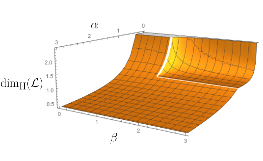
Figure 2: The plot represents the Hausdorff dimension of the leaves as a function of α\alpha and β\beta, the dimension dd being fixed to 11. The expression obtained for β>1\beta>1 and α<1d\alpha<\frac{1}{d} can be rewritten as d+(β−α​d−β−1)2α\displaystyle d+\frac{(\sqrt{\beta-\alpha d}-\sqrt{\beta-1})^{2}}{\alpha} This expression is always larger than dd and smaller than 1α\frac{1}{\alpha}, and it is decreasing in α\alpha and β\beta on the domain on which we consider it. When β→1\beta\rightarrow 1, it converges to the value 1α\frac{1}{\alpha} so that the function (α,β)↦dimH(ℒ)(\alpha,\beta)\mapsto\dim_{H}(\mathcal{L}) is continuous on the domain ℝ+∗×ℝ\mathbb{R}^{*}_{+}\times\mathbb{R}.

Remark that for β>1\beta>1 the dimension of the set ℒ\mathcal{L} depends on the geometry of the underlying random block through dd, its dimension. For β≤1\beta\leq 1, it is not the case, and actually the theorem remains true under much weaker hypotheses for the distribution of (𝖡,𝖣,ρ,ν)(\mathsf{B},\mathsf{D},\rho,\nu), namely that ν\nu is not almost surely concentrated on {ρ}\{\rho\}, and that ∀k≥0,𝔼⁡[(diam⁡(𝖡))k]<∞\forall k\geq 0,\mathbb{E}\left[(\diam(\mathsf{B}))^{k}\right]<\infty, where diam⁡(⋅)\diam(\cdot) denotes the diameter of a metric space. We could even replace the assumption that the blocks ((,,,,,,,))n≥1\left((\mathsf{B}_{n},\mathsf{D}_{n},\rho_{n},\nu_{n})\right)_{n\geq 1} are i.i.d. by some weaker assumption but we do not do it for the sake of clarity. The proofs when β≤1\beta\leq 1 are quite short and the interested reader can easily generalise them to a more general setting.

Hypotheses of the theorem

Let us define and discuss the precise hypotheses of our theorem. First, let us describe the assumptions that we make on the sequences (λn)(\lambda_{n}) and (wn)(w_{n}). We define

Wn=∑k=1nwk,W_{n}=\sum_{k=1}^{n}w_{k},

and for all ϵ>0\epsilon>0, we set

Gϵ:={k≥1|wk≥k−β−ϵ,λk≥k−α−ϵ},G^{\epsilon}:=\left\{k\geq 1\mathrel{}\middle|\mathrel{}w_{k}\geq k^{-\beta-\epsilon},\ \lambda_{k}\geq k^{-\alpha-\epsilon}\right\}, (2)

and also

Gnϵ:={k∈⟦n,2n⟧|wk≥n−β−ϵ,λk≥n−α−ϵ}.G_{n}^{\epsilon}:=\left\{k\in\mathopen{\llbracket}n\mathclose{}\mathpunct{},2n\mathclose{\rrbracket}\mathrel{}\middle|\mathrel{}w_{k}\geq n^{-\beta-\epsilon},\ \lambda_{k}\geq n^{-\alpha-\epsilon}\right\}. (3)

As said earlier, we separate the case β<1\beta<1, the case β>1\beta>1 and the case β=1\beta=1.

Hypothesis ○α,β\bigcirc_{\alpha,\beta}.

We have α>0\alpha>0 and β<1\beta<1 and for all n≥1,λn≤n−α+o(1)n\geq 1,\ \lambda_{n}\leq n^{-\alpha+o\mathopen{}\left(1\right)} and wn≤n−β+o(1)w_{n}\leq n^{-\beta+o\mathopen{}\left(1\right)}. Furthermore Wn=n1−β+o(1)W_{n}=n^{1-\beta+o\mathopen{}\left(1\right)} and for all ϵ>0\epsilon>0,

lim infn→∞∑k=1nwk𝟏{k∈Gϵ}∑k=1nwk>0.\liminf_{n\rightarrow\infty}\frac{\sum_{k=1}^{n}w_{k}\mathbf{1}_{\left\{k\in G^{\epsilon}\right\}}}{\sum_{k=1}^{n}w_{k}}>0.

The last display ensures that for all ϵ>0\epsilon>0, the set GϵG^{\epsilon} contains asymptotically a positive proportion of the total weight.

Hypothesis ⋄α,β\diamond_{\alpha,\beta}.

We have α>0\alpha>0 and β>1\beta>1 and for all n≥1,λn≤n−α+o(1)n\geq 1,\ \lambda_{n}\leq n^{-\alpha+o\mathopen{}\left(1\right)} and wn≤n−β+o(1)w_{n}\leq n^{-\beta+o\mathopen{}\left(1\right)}. Furthermore, for all ϵ>0\epsilon>0,

#Gnϵ=n→∞n1+o(1).\#G_{n}^{\epsilon}\underset{n\rightarrow\infty}{=}n^{1+o\mathopen{}\left(1\right)}.

Under the stronger assumption λn=n−α+o(1)\lambda_{n}=n^{-\alpha+o\mathopen{}\left(1\right)} and wn=n−β+o(1)w_{n}=n^{-\beta+o\mathopen{}\left(1\right)}, Hypothesis ⋄ α , β holds if β>1\beta>1 (resp. Hypothesis ○ α , β , if β<1\beta<1). The case β=1\beta=1 is slightly different and in this case we set

Hypothesis □α,1\square_{\alpha,1}.

We have α>0\alpha>0 and β=1\beta=1 and for all n≥1,λn≤n−α+o(1)n\geq 1,\ \lambda_{n}\leq n^{-\alpha+o\mathopen{}\left(1\right)} and wn≤n−1+o(1)w_{n}\leq n^{-1+o\mathopen{}\left(1\right)}. Furthermore, for all ϵ>0\epsilon>0,

1log⁡log⁡log⁡N∑k=NN1+ϵwkWk𝟏{k∈Gϵ}⟶N→∞+∞.\frac{1}{\log\log\log N}\sum_{k=N}^{N^{1+\epsilon}}\frac{w_{k}}{W_{k}}\mathbf{1}_{\left\{k\in G^{\epsilon}\right\}}\underset{N\rightarrow\infty}{\longrightarrow}+\infty.

Note that this last hypothesis requires in particular that Wn→∞W_{n}\rightarrow\infty as n→∞n\rightarrow\infty. Now let us define Hypothesis H d , for any d≥0d\geq 0, which will ensure that our random underlying block has the appropriate dd-dimensional behaviour.

Hypothesis HdH_{d}.

The law of the block (𝖡,𝖣,ρ,ν)(\mathsf{B},\mathsf{D},\rho,\nu) satisfies the following conditions:

  1. (i)

    ∙\bulletIf d=0d=0, the block 𝖡\mathsf{B} is a finite metric space which is not a.s. reduced to a single point and such that the measure ν\nu satisfies ν⁡({x})>0\nu(\{x\})>0, for all points x∈𝖡x\in\mathsf{B}.

    ∙\bulletIf d>0d>0, there exists an increasing function φ:[0,1]→[0,d/2]\varphi:\mathopen{[}0\mathclose{}\mathpunct{},1\mathclose{]}\rightarrow\mathopen{[}0\mathclose{}\mathpunct{},d/2\mathclose{]}, satisfying limr→0φ⁡(r)=0\displaystyle\lim_{r\rightarrow 0}\varphi(r)=0, such that almost surely, there exists a (random) r0∈(0,1)r_{0}\in\mathopen{(}0\mathclose{}\mathpunct{},1\mathclose{)} such that

    ∀r∈[0,r0),∀x∈𝖡,rd+φ⁡(r)≤ν(B(x,r))≤rd−φ⁡(r).\forall r\in\mathopen{[}0\mathclose{}\mathpunct{},r_{0}\mathclose{)},\ \forall x\in\mathsf{B},\ \quad r^{d+\varphi(r)}\leq\nu\left(\Ball(x,r)\right)\leq r^{d-\varphi(r)}. (⋆r0\star_{r_{0}})
  2. (ii)

    Let Nr​(𝖡)N_{r}(\mathsf{B}) be the minimal number of balls of radius rr needed to cover 𝖡\mathsf{B}. Then

    𝔼[Nr(𝖡)]≤r−d+o(1)asr→0.\mathbb{E}\left[N_{r}(\mathsf{B})\right]\leq r^{-d+o\mathopen{}\left(1\right)}\quad\text{as}\quad r\rightarrow 0.
  3. (iii)

    For all k≥0k\geq 0, we have 𝔼⁡[diam⁡(𝖡)k]<∞\mathbb{E}\left[\diam(\mathsf{B})^{k}\right]<\infty.

Here B⁡(x,r)\Ball(x,r) is the open ball centred at xx with radius rr and the notation diam⁡(𝖡)\diam(\mathsf{B}) denotes the diameter of 𝖡\mathsf{B}, defined as the maximal distance between two points of 𝖡\mathsf{B}. The conditions (i) and (ii) ensure that the blocks that we glue together have dimension dd. The condition (iii) ensures that the blocks cannot be too big. In the paper, some results are stated under some weaker assumptions on the distribution of random block (𝖡,𝖣,ρ,ν)(\mathsf{B},\mathsf{D},\rho,\nu) and they are hence all still valid under Hypothesis H d .

Motivations

The assumptions of Theorem 1 are rather general and various known models fall into our setting. First, let us cite two constructions that were already covered by the work presented in [7]. Of course we have Aldous’ line-breaking construction of the CRT but let us also cite the work of Ross and Wen in [19], in which the authors study a discrete model of growing trees and prove that its scaling limit can be described as a line-breaking procedure à la Aldous using a Poisson process of intensity tl​d​tt^{l}\mathrm{d}t, with ll an integer. The Hausdorff dimension of the resulting tree is then (l+1)/l(l+1)/l. Our extended setting now also includes the Brownian looptree, defined in [6], which appears as the scaling limit of the so-called discrete looptree associated with Barabási-Albert model. This random metric space also has a natural construction through an aggregation of circles, and our theorem proves that this object has almost surely Hausdorff dimension 22. These examples do not really use our theorem in its full generality since their underlying block is deterministic. In fact, Hypothesis H d is very general and is satisfied (for the appropriate d≥0d\geq 0) by many distributions of blocks, including the Brownian CRT (d=2d=2), see [8], the Brownian map (d=4d=4), see [20, 15], the θ\theta-stable trees (d=θ+1θd=\frac{\theta+1}{\theta}), see [9]. Hence, our results can apply to a whole variety of such constructions, with a very general distributions for the blocks, and we are currently working on some examples in which this construction naturally arises as the limit of discrete models.

Indications on the proofs

The computations of the dimension in Theorem 1 differ, depending on the assumptions we make on α\alpha and β\beta, and always consist of an upper bound, that we derive by providing explicit coverings, and a lower bound that arises from the construction of a probability measure satisfying the assumptions of Frostman’s lemma, see Lemma 20 in the Appendix for a statement.

If we just assume that the scaling factors are smaller than n−α+o(1)n^{-\alpha+o\mathopen{}\left(1\right)}, we can prove that the dimension is bounded above by 1α\frac{1}{\alpha} for rather general behaviours of the weights. To do so, we adapt arguments from [7] to our new setting. The essential idea behind the proof is that the sub-structure descending from a block 𝐛n\mathbf{b}_{n} has size n−α+o(1)n^{-\alpha+o\mathopen{}\left(1\right)}, and so that one only needs to cover every block 𝐛n\mathbf{b}_{n} with a ball of radius n−α+o(1)n^{-\alpha+o\mathopen{}\left(1\right)} to cover the whole structure.

When α<1d\alpha<\frac{1}{d} and β>1\beta>1, although the sub-structure descending from a block 𝐛n\mathbf{b}_{n} may have diameter of order n−α+o(1)n^{-\alpha+o\mathopen{}\left(1\right)}, we can also check that the index of the first block glued on block nn has index roughly nβn^{\beta}, which is large compared to nn. Hence the diameter of the substructure descending from 𝐛n\mathbf{b}_{n} is essentially due to 𝐛n\mathbf{b}_{n} itself. This gives us a hint that we can cover the whole substructure descending from the block 𝐛n\mathbf{b}_{n}, using a covering of 𝐛n\mathbf{b}_{n} with balls that are really small compared to the size of 𝐛n\mathbf{b}_{n}, and that it would lead to a more optimal covering. In fact we use these two observations to recursively construct a sequence of finer and finer coverings, which lead to the optimal upper-bound. The idea of the proof is presented in more details in Section 4.2.1.

Concerning the lower bounds, for all values of α\alpha and β\beta, we can define a natural probability measure μ¯\bar{\mu} on 𝒯\mathcal{T} as the limit of (a normalised version of) the measure μn\mu_{n} defined on 𝒯n\mathcal{T}_{n} for every n≥1n\geq 1, see Section 3. In the case β≤1\beta\leq 1, this probability measure only charges the leaves of 𝒯\mathcal{T}, and an application of Lemma 20 gives the lower bound 1α\frac{1}{\alpha}.

For β>1\beta>1, the measure μ¯\bar{\mu} does not charge the leaves and so the preceding argument does not work. We construct another measure as the sub-sequential limit of a sequence of measures (πk)(\pi_{k}) which are concentrated on sets of the form (𝒯2​nk∖𝒯nk)\left(\mathcal{T}_{2n_{k}}\setminus\mathcal{T}_{n_{k}}\right) with (nk)(n_{k}) chosen appropriately, see Section 5.2.1 for a presentation of the idea of the proof. The limiting measure is then concentrated on a strict subset of leaves and again, using Lemma 20 yields the appropriate lower bound.

Related constructions

Let us also cite some other models that have been studied in the literature and which share some features with ours. First, the line-breaking construction of the scaling limit of critical random graphs in [2] by Addario-Berry, Broutin and Goldschmidt, that of the stable trees in [11] by Goldschmidt and Haas, and that of the stable graphs in [12] by Goldschmidt, Haas and Sénizergues, use a gluing procedure that is identical to ours. Their constructions are not directly handled by Theorem 1 but they fall in a slightly more general setting, for which our proofs still hold. In [5], Borovkov and Vatutin study a discrete tree constructed recursively, which corresponds to the "genealogical tree" of the blocks in our model. Last, in [18], Rembart and Winkel study the distribution of random trees that satisfy a self-similarity condition (in law). They provide an iterative construction of those trees in which infinitely many branches are glued at each step.

Plan of the paper

In Section 2, we give a rigorous definition of our model, set up some useful notation, and discuss some general properties. In the second section, we study the (normalised) natural measure μ¯n\bar{\mu}_{n} on 𝒯n\mathcal{T}_{n} and prove that it converges to a measure μ¯\bar{\mu} on 𝒯\mathcal{T} under suitable assumptions. In Section 4.1, we prove the almost sure compactness of 𝒯\mathcal{T} and some upper-bounds on its Hausdorff dimension under some relatively weak hypotheses. In Section 4.2, we develop a new (more involved) approach that allows us to obtain a better upper-bound for some parameters for which the former fails to be optimal. In Section 5, we prove the lower bounds that match the upper-bounds obtained in Section 4. It is again divided in two subsections, each providing a proof that is only valid for some choices of parameters α\alpha and β\beta. The Appendix A.2 contains a short reminder of basic properties concerning Hausdorff dimension. The Appendices A.1, A.3 and A.4 contain some technical proofs that can be skipped at first reading.

Acknowledgements

The authors would like to thank the anonymous referees for their valuable comments which helped to improve the presentation of the manuscript.

2 General framework

In this section, we start by providing a precise definition of our model and then we investigate some of its general properties.

2.1 Construction

Consider ((,,,,,,,))n≥1((\mathbf{b}_{n},\mathbf{d}_{n},\boldsymbol{\rho}_{n},\boldsymbol{\nu}_{n}))_{n\geq 1} a sequence of compact pointed metric spaces endowed with a finite Borel measure. Recall from the introduction the heuristics of our recursive construction. We define 𝒯1\mathcal{T}_{1} as the first block 𝐛1\mathbf{b}_{1} endowed with its measure 𝝂1\boldsymbol{\nu}_{1}. Then at each step, we construct 𝒯n+1\mathcal{T}_{n+1} from 𝒯n\mathcal{T}_{n} by gluing the root of the block 𝐛n+1\mathbf{b}_{n+1} to a random point Xn∈𝒯nX_{n}\in\mathcal{T}_{n}, which has distribution (a normalised version of) μn\mu_{n}. The measure μn+1\mu_{n+1} is defined as the sum of the measures μn\mu_{n} and 𝝂n+1\boldsymbol{\nu}_{n+1}, the measure supported by 𝐛n+1\mathbf{b}_{n+1}. We define 𝒯∗\mathcal{T}^{*} as the increasing union of all the 𝒯n\mathcal{T}_{n} for n≥1n\geq 1, and its completion is denoted 𝒯\mathcal{T}. In the next paragraph, we describe formally how to construct such growing metric spaces as subsets of a larger ambient space. The definitions here are rather technical and the proofs in the paper do not use the details of the construction, so the reader can skip this part at first reading.

Embedded construction

We consider (U,δ)(U,\delta) the Urysohn space, and fix a point u0∈Uu_{0}\in U. The space UU is defined as the only Polish metric space (up to isometry) which has the following extension property (see [14] for constructions and basic properties of UU): given any finite metric space XX, and any point x∈Xx\in X, any isometry from X∖{x}X\setminus\{x\} to UU can be extended to an isometry from XX to UU. In the rest of the construction, we assume that the measured metric spaces ((,,,,,,,))n≥1((\mathbf{b}_{n},\mathbf{d}_{n},\boldsymbol{\rho}_{n},\boldsymbol{\nu}_{n}))_{n\geq 1} are all embedded in the space UU and that their root is identified to u0u_{0}. From the properties of the Urysohn space, this is always possible (see Appendix A.1 for a construction in the case of random blocks).

We introduce

ℓ1​(U,u0):={(xn)n≥1∈Uℕ∗|∑n=1∞δ⁡(xn,u0)<+∞}.\ell^{1}(U,u_{0}):=\left\{(x_{n})_{n\geq 1}\in U^{\mathbb{N}^{*}}\mathrel{}\middle|\mathrel{}\sum_{n=1}^{\infty}\delta(x_{n},u_{0})<+\infty\right\}.

If we endow ℓ1​(U,u0)\ell^{1}(U,u_{0}) with the distance d⁡((xn)n≥1,(yn)n≥1)=∑n=1∞δ⁡(xn,yn)\dist((x_{n})_{n\geq 1},(y_{n})_{n\geq 1})=\sum_{n=1}^{\infty}\delta(x_{n},y_{n}), it is an easy exercise to see that it makes this space Polish. We can now construct the 𝒯n\mathcal{T}_{n} recursively, by 𝒯1={(x,u0,u0,…)|x∈𝐛1}\mathcal{T}_{1}=\left\{(x,u_{0},u_{0},\dots)\mathrel{}\middle|\mathrel{}x\in\mathbf{b}_{1}\right\}, and identifying 𝒯1\mathcal{T}_{1} to the block 𝐛1\mathbf{b}_{1}, we set μ1=𝝂1\mu_{1}=\boldsymbol{\nu}_{1}. For n≥1n\geq 1, the point XnX_{n} is sampled according to μ¯n\bar{\mu}_{n} a normalised version of μn\mu_{n} with total mass 11. The point XnX_{n} is of the form (x1(n),x2(n),…,xn(n),u0,…)\left(x_{1}^{(n)},x_{2}^{(n)},\dots,x_{n}^{(n)},u_{0},\dots\right) and we set

𝒯n+1:=𝒯n∪{(x1(n),x2(n),…​xn(n),x,u0​…)|x∈𝐛n+1}.\mathcal{T}_{n+1}:=\mathcal{T}_{n}\cup\left\{\left(x_{1}^{(n)},x_{2}^{(n)},\dots x_{n}^{(n)},x,u_{0}\dots\right)\mathrel{}\middle|\mathrel{}x\in\mathbf{b}_{n+1}\right\}.

We set μn+1:=μn+𝝂n\mu_{n+1}:=\mu_{n}+\boldsymbol{\nu}_{n}, where as in the preceding section, we see 𝐛n+1\mathbf{b}_{n+1} as the corresponding subset of 𝒯n+1\mathcal{T}_{n+1}. Then 𝒯∗=⋃n≥1𝒯n\mathcal{T}^{*}=\bigcup_{n\geq 1}\mathcal{T}_{n} and 𝒯=(𝒯∗)¯\mathcal{T}=\overline{(\mathcal{T}^{*})} is its closure in the space (ℓ1​(U,u0),d)(\ell^{1}(U,u_{0}),\dist). At the end 𝒯\mathcal{T} is a random closed subset of a Polish space.

In the rest of the paper, we will not refer to this formal construction of 𝒯\mathcal{T} and we will identify 𝐛n\mathbf{b}_{n} with the corresponding subset in 𝒯\mathcal{T}. We recall the notation Wn=∑k=1nwnW_{n}=\sum_{k=1}^{n}w_{n} for the total mass of the measure μn\mu_{n}.

2.2 Some notation

Figure 3: Substructure descending from a set, and projection on a substructure, illustrating some notation introduced in the paper in the case of the gluing of segments.

Let us introduce some notation that will be useful in the sequel, some of which is illustrated in Figure 3. Recall that from now on, we always assume that the blocks are of the form (1).

∙\bullet If (E,d,ρ)(E,\dist,\rho) is a pointed metric space, and x∈Ex\in E, we define ht⁡(x)\haut(x), the height of xx, as its distance to the root d⁡(ρ,x)\dist(\rho,x). We also denote ht⁡(E)=supx∈Eht⁡(x)\haut(E)=\sup_{x\in E}\haut(x), the height of EE. Let us consider (𝖡,𝖣,ρ,ν)(\mathsf{B},\mathsf{D},\rho,\nu), a random block of our model before scaling, and XX a point of 𝖡\mathsf{B} which conditionally on (𝖡,𝖣,ρ,ν)(\mathsf{B},\mathsf{D},\rho,\nu), has distribution ν\nu. We denote

ℋ:=ht⁡(X)=𝖣⁡(ρ,X),\mathcal{H}:=\haut(X)=\mathsf{D}(\rho,X), (4)

the height of a uniform random point in the block. Remark that Hypothesis H d implies that 𝔼⁡[ℋ2]<∞\mathbb{E}\left[\mathcal{H}^{2}\right]<\infty, and that ℙ⁡(ℋ>0)>0\mathbb{P}\left(\mathcal{H}>0\right)>0. Some of our results are stated under these weaker assumptions.

∙\bullet Whenever we sample the point XnX_{n} under μ¯n\bar{\mu}_{n}, we do it in the following way: first we sample KnK_{n} such that for all 1≤k≤n1\leq k\leq n, ℙ⁡(Kn=k)=wkWn\mathbb{P}\left(K_{n}=k\right)=\frac{w_{k}}{W_{n}} and then, conditionally on Kn=kK_{n}=k, the point XnX_{n} is chosen on the block 𝐛k\mathbf{b}_{k} using the normalised version of the measure 𝝂k\boldsymbol{\nu}_{k}. Whenever Kn=kK_{n}=k, we say that 𝐛n+1\mathbf{b}_{n+1} is grafted onto 𝐛k\mathbf{b}_{k} and write 𝐛n+1→𝐛k\mathbf{b}_{n+1}\rightarrow\mathbf{b}_{k}. Remark that this entails that Xn∈𝐛kX_{n}\in\mathbf{b}_{k}, but this condition is not sufficient in the case where XnX_{n} belongs to several blocks (which only happens if the measures carried by the blocks have atoms). We denote

μ¯n∗:=law of ​(Kn,Xn),\displaystyle\bar{\mu}_{n}^{*}:=\text{law of }(K_{n},X_{n}), (5)

seen as a measure on ⨆k=1n{k}×𝐛k\bigsqcup_{k=1}^{n}\{k\}\times\mathbf{b}_{k}. In this way, the random variables ((Kn,Xn))n≥1((K_{n},X_{n}))_{n\geq 1} are independent with respective distributions (μ¯n∗)n≥1(\bar{\mu}_{n}^{*})_{n\geq 1}. We remain loose on the fact that we sometimes consider the blocks as abstract metric spaces and at other times we see them as subsets of 𝒯\mathcal{T}. It is implicit in the preceding discussion that everything is expressed conditionally on the sequence of blocks (𝐛n)n≥1(\mathbf{b}_{n})_{n\geq 1}.

∙\bullet We simultaneously construct a sequence of increasing discrete trees (𝖳n)n≥1(\mathsf{T}_{n})_{n\geq 1} by saying that for n≥1n\geq 1, the tree 𝖳𝗇\mathsf{T_{n}} has nn nodes labelled 11 to nn and ii is a child of jj if and only if 𝐛i→𝐛j\mathbf{b}_{i}\rightarrow\mathbf{b}_{j}. Also define 𝖳\mathsf{T} their increasing union. We denote ≺\prec the genealogical order on ℕ∗\mathbb{N}^{*} induced by this tree. We denote d𝖳⁡(i,j)\dist_{\mathsf{T}}(i,j) for the graph distance between the nodes with label ii and jj in this tree and ht𝖳⁡(⋅)\haut_{\mathsf{T}}(\cdot) for their height.

∙\bullet For x∈𝒯x\in\mathcal{T}, we define [x]n[x]_{n}, the projection of xx on 𝒯n\mathcal{T}_{n}, as the unique point yy of 𝒯n\mathcal{T}_{n} that minimizes the distance d⁡(x,y)\dist(x,y).

∙\bullet Similarly, for k≥1k\geq 1, we define [k]n[k]_{n}, the projection of kk on 𝖳n\mathsf{T}_{n}, as the unique node i≤ni\leq n that minimizes the distance d𝖳⁡(i,k)\dist_{\mathsf{T}}(i,k).

∙\bullet If SS is a subset of a block 𝐛n\mathbf{b}_{n} for some n≥1n\geq 1 then we define 𝒯⁡(S)\mathcal{T}(S), the substructure descending from SS as

𝒯⁡(S):=S∪⋃i≻n[Xi−1]n∈S​𝐛i¯.\mathcal{T}(S):=\overline{S\cup\underset{[X_{i-1}]_{n}\in S}{\bigcup_{i\succ n}}\mathbf{b}_{i}}.

If S=𝐛nS=\mathbf{b}_{n}, this reduces to

𝒯⁡(𝐛n)=⋃i⪰n𝐛i¯,\mathcal{T}(\mathbf{b}_{n})=\overline{\bigcup_{i\succeq n}\mathbf{b}_{i}},

and we consider (𝒯⁡(𝐛n),d,𝝆n)(\mathcal{T}(\mathbf{b}_{n}),\dist,\boldsymbol{\rho}_{n}) as a rooted metric space.

∙\bullet Remark that if x∈𝒯⁡(𝐛k)x\in\mathcal{T}(\mathbf{b}_{k}) for some k≥1k\geq 1 then we have [x]k∈𝐛k[x]_{k}\in\mathbf{b}_{k} and more generally, for any n≤kn\leq k, we have [x]n∈𝐛[k]n[x]_{n}\in\mathbf{b}_{[k]_{n}}.

∙\bullet We often use the little-o notation and denote o(1)o\mathopen{}\left(1\right) a deterministic function that tends to 00 when some parameter tends to 00 or ∞\infty, depending on the context. For such functions that are random, we write instead oω(1)o^{\omega}\mathopen{}\left(1\right).

2.3 Zero-One law for compactness, boundedness and Hausdorff dimension

The main properties of 𝒯\mathcal{T} and ℒ\mathcal{L} that we study are compactness and Hausdorff dimension. One can check that some of these properties are constants almost surely by an argument using Kolmogorov’s zero-one law.

Indeed, take the whole construction 𝒯\mathcal{T} and contract the compact subspace 𝒯n\mathcal{T}_{n} into a single point. We can easily check that the resulting space is compact (resp. bounded) iff the former is compact (resp. bounded). Also, the subset ℒ\mathcal{L} and its image after the contraction of 𝒯n\mathcal{T}_{n} have the same Hausdorff dimension. Now remark that the space that we just described only depends on the randomness of the blocks and the gluings after nn steps. Indeed, if we start at time nn with a unique point with weight WnW_{n} and then follow the procedure by gluing recursively 𝐛n+1,𝐛n+2,…\mathbf{b}_{n+1},\ \mathbf{b}_{n+2},\dots, we get exactly the same space.

Hence, as this is true for all nn, these properties only depend on the tail σ\sigma-algebra generated by the blocks and the gluings, and are therefore satisfied with probability 00 or 11.

Remark 2.

In the setting of [7], where the blocks are segments and the weights correspond to the lengths of those segments, the authors proved that the event of boundedness and compactness for 𝒯\mathcal{T} coincide almost surely. This is not the case in our more general setting: consider the case of branches with weights and lengths defined as

wn\displaystyle w_{n} =2n,λn=2−nfor n∉{2k|k∈ℕ},\displaystyle=2^{n},\ \lambda_{n}=2^{-n}\quad\text{for $n\notin\left\{2^{k}\mathrel{}\middle|\mathrel{}k\in\mathbb{N}\right\}$},
w2k\displaystyle w_{2^{k}} =1,λ2k=1,for k∈ℕ.\displaystyle=1,\ \lambda_{2^{k}}=1,\quad\text{for $k\in\mathbb{N}$.}

In this case, an application of Borel-Cantelli lemma shows that a.s. for nn large enough, no branch 𝐛n\mathbf{b}_{n} is ever grafted onto a branch 𝐛2k\mathbf{b}_{2^{k}} for any kk. It is then clear that the resulting tree is a.s. bounded since the sum of the lengths of the branches 𝐛n\mathbf{b}_{n} for n∉{2k∣k∈ℕ}n\notin\{2^{k}\mid k\in\mathbb{N}\} is finite, but it cannot be compact since there exists an infinite number of branches with length 11.

2.4 Monotonicity of Hausdorff dimension

Let us present an argument of monotonicity of the Hausdorff dimension of ℒ\mathcal{L} with respect to the sequence (λn)(\lambda_{n}), on the event on which 𝒯\mathcal{T} is compact. Let (wn)(w_{n}) be a sequence of weights and (λn)(\lambda_{n}) and (λn′)(\lambda^{\prime}_{n}) be two sequences of scaling factors such that for all n≥1n\geq 1, we have λn≥λn′\lambda_{n}\geq\lambda^{\prime}_{n}. Suppose that ((,,,,,,,))n≥1\left((\mathsf{B}_{n},\mathsf{D}_{n},\rho_{n},\nu_{n})\right)_{n\geq 1} is a sequence of random compact metric spaces endowed with a probability measure. Then, let 𝒯\mathcal{T} (resp. 𝒯′\mathcal{T}^{\prime}) be the structure constructed using the blocks (𝐛n,𝐝n,𝝆n,𝝂n)=(𝖡n,λn⋅𝖣n,ρn,wn⋅νn)(\mathbf{b}_{n},\mathbf{d}_{n},\boldsymbol{\rho}_{n},\boldsymbol{\nu}_{n})=(\mathsf{B}_{n},\lambda_{n}\cdot\mathsf{D}_{n},\rho_{n},w_{n}\cdot\nu_{n}), for n≥1n\geq 1, (resp. OPEN(𝐛n′,𝐝n′,𝝆n′,𝝂n′)=(𝖡n,λn′⋅𝖣n,ρn,wn⋅νn))(\mathbf{b}_{n}^{\prime},\mathbf{d}_{n}^{\prime},\boldsymbol{\rho}_{n}^{\prime},\boldsymbol{\nu}_{n}^{\prime})=(\mathsf{B}_{n},\lambda^{\prime}_{n}\cdot\mathsf{D}_{n},\rho_{n},w_{n}\cdot\nu_{n})). Note that since we use the same sequence of weights we can couple the two corresponding gluing procedures.

Let ff be the application that maps each of the block 𝐛n\mathbf{b}_{n} to the corresponding 𝐛n′\mathbf{b}^{\prime}_{n}. Recall here that we see the blocks as subsets of the structure. We can verify that f:𝒯∗⟶(𝒯′)∗f:\mathcal{T}^{*}\longrightarrow(\mathcal{T}^{\prime})^{*}, is 11-Lipschitz. We can then extend uniquely ff to a function f^:𝒯⟶𝒯′\hat{f}:\mathcal{T}\longrightarrow\mathcal{T}^{\prime}, which is also 11-Lipschitz. Suppose 𝒯\mathcal{T} is compact. Then its image f^​(𝒯)\hat{f}(\mathcal{T}) is compact, hence closed in 𝒯′\mathcal{T}^{\prime}. Since (𝒯′)∗⊂f^​(𝒯)(\mathcal{T}^{\prime})^{*}\subset\hat{f}(\mathcal{T}) and (𝒯′)∗(\mathcal{T}^{\prime})^{*} is dense in 𝒯′\mathcal{T}^{\prime}, we have f^​(𝒯)=𝒯′\hat{f}(\mathcal{T})=\mathcal{T}^{\prime} and so f^\hat{f} is surjective. Now since (𝒯′)∗=f^​(𝒯∗)(\mathcal{T}^{\prime})^{*}=\hat{f}(\mathcal{T}^{*}), we also have ℒ′=f^​(ℒ)\mathcal{L}^{\prime}=\hat{f}(\mathcal{L}), and since f^\hat{f} is Lipschitz,

dimH​(ℒ′)≤dimH​(ℒ).\mathrm{dim_{H}}(\mathcal{L}^{\prime})\leq\mathrm{dim_{H}}(\mathcal{L}). (6)

3 Study of a typical point

In this section we study the height of a typical point of 𝒯n\mathcal{T}_{n}, i.e. the distance from the root to a point sampled according to μ¯n\bar{\mu}_{n}. The proofs in this section are really close to those of [7, Section 1], to which we refer for details.

3.1 Coupling with a marked point

We construct a sequence of points (Yn)n≥1(Y_{n})_{n\geq 1} coupled with the sequence (𝒯n)n≥1(\mathcal{T}_{n})_{n\geq 1} in such a way that for all n≥1n\geq 1, the point YnY_{n} has distribution μ¯n\bar{\mu}_{n} conditionally on 𝒯n\mathcal{T}_{n} and such that the distance from YnY_{n} to the root is non-decreasing in nn. For technical reasons, we in fact define a sequence ((Jn,Yn))n≥1((J_{n},Y_{n}))_{n\geq 1} such that for any n≥1n\geq 1, (Jn,Yn)(J_{n},Y_{n}) has distribution μ¯n∗\bar{\mu}_{n}^{*} conditionally on (𝖳n,𝒯n)(\mathsf{T}_{n},\mathcal{T}_{n}), see (5). The properties of this construction are stated in the following lemma.

Lemma 3.

We can couple the construction of ((𝖳n,𝒯n))n≥1((\mathsf{T}_{n},\mathcal{T}_{n}))_{n\geq 1} with a sequence ((Jn,Yn))n≥1((J_{n},Y_{n}))_{n\geq 1} such that for all n≥1n\geq 1,

  1. (i)

    we have Jn∈{1,…,n}J_{n}\in\{1,\dots,n\} and Yn∈𝐛JnY_{n}\in\mathbf{b}_{J_{n}},

  2. (ii)

    conditionally on (𝖳n,𝒯n)(\mathsf{T}_{n},\mathcal{T}_{n}), the couple (Jn,Yn)(J_{n},Y_{n}) has distribution μ¯n∗\bar{\mu}_{n}^{*},

  3. (iii)

    for all 1≤k≤n1\leq k\leq n, ([Jn]k,[Yn]k)=(Jk,Yk)([J_{n}]_{k},[Y_{n}]_{k})=(J_{k},Y_{k}).

Furthermore, under the assumption H d (iii), the sequence (Yn)n≥1(Y_{n})_{n\geq 1} almost surely converges in 𝒯\mathcal{T} iff

∑n=1∞λn​wnWn𝟏{λn≤1}<∞and∑n=1∞wnWn𝟏{λn>1}<∞.\sum_{n=1}^{\infty}\frac{\lambda_{n}w_{n}}{W_{n}}\mathbf{1}_{\left\{\lambda_{n}\leq 1\right\}}<\infty\quad\text{and}\quad\sum_{n=1}^{\infty}\frac{w_{n}}{W_{n}}\mathbf{1}_{\left\{\lambda_{n}>1\right\}}<\infty. (7)

Note that if either

W∞:=∑n=1∞wn<∞or∑n=1∞wn​λnWn<∞,W_{\infty}:=\sum_{n=1}^{\infty}w_{n}<\infty\quad\text{or}\quad\sum_{n=1}^{\infty}\frac{w_{n}\lambda_{n}}{W_{n}}<\infty,

then (7) is satisfied, and this is the case under the assumptions of Theorem 1. In this case we let

Y:=limn→∞Yn.Y:=\lim_{n\rightarrow\infty}Y_{n}.
Proof.

Let n≥2n\geq 2. Conditionally on 𝒯n\mathcal{T}_{n} and 𝖳n\mathsf{T}_{n}, sample a couple (Jn,Yn)(J_{n},Y_{n}) under the measure μ¯n∗\bar{\mu}_{n}^{*}. Then two cases may happen:

  • •

    with probability 1−wn/Wn1-w_{n}/W_{n} : we have Jn<nJ_{n}<n, so the point YnY_{n} belongs to 𝒯n−1\mathcal{T}_{n-1}, that is [Yn]n−1=Yn[Y_{n}]_{n-1}=Y_{n} , and conditionally on this event ([Jn]n−1,[Yn]n−1)([J_{n}]_{n-1},[Y_{n}]_{n-1}) has the same distribution as (Jn−1,Yn−1)(J_{n-1},Y_{n-1}),

  • •

    with probability wn/Wnw_{n}/W_{n} : we have Jn=nJ_{n}=n. In this case the point YnY_{n} is located on the last block 𝐛n\mathbf{b}_{n} grafted on 𝒯n−1\mathcal{T}_{n-1}. Conditionally on this event (if wn>0w_{n}>0), YnY_{n} is distributed on this block under the measure 𝝂n\boldsymbol{\nu}_{n} and the couple ([Jn]n−1,[Yn]n−1)([J_{n}]_{n-1},[Y_{n}]_{n-1}) is independent of the location of YnY_{n} on the nn-th block and has the same distribution as (Jn−1,Yn−1)(J_{n-1},Y_{n-1}).

From this observation we deduce that

(𝒯n−1,𝖳n−1,[Jn]n−1,[Yn]n−1)=(𝒯n−1,𝖳n−1,Jn−1,Yn−1)(\mathcal{T}_{n-1},\mathsf{T}_{n-1},[J_{n}]_{n-1},[Y_{n}]_{n-1})=(\mathcal{T}_{n-1},\mathsf{T}_{n-1},J_{n-1},Y_{n-1})

in distribution and more generally, (𝒯k,𝖳k,[Jn]k,[Yn]k)=(𝒯k,𝖳k,Jk,Yk)(\mathcal{T}_{k},\mathsf{T}_{k},[J_{n}]_{k},[Y_{n}]_{k})=(\mathcal{T}_{k},\mathsf{T}_{k},J_{k},Y_{k}) in distribution for all 1≤k≤n1\leq k\leq n.

Reversing this observation, we can construct a sequence (Jn,Yn)n≥1(J_{n},Y_{n})_{n\geq 1} (coupled to the KnK_{n} and XnX_{n} involved in the construction of 𝒯∗\mathcal{T}^{*}) such that conditionally on 𝒯n\mathcal{T}_{n} and 𝖳n\mathsf{T}_{n}, the couple (Jn,Yn)(J_{n},Y_{n}) has distribution μ¯n∗\bar{\mu}^{*}_{n} and that for all 1≤k≤n1\leq k\leq n, we have ([Jn]k,[Yn]k)=(Jk,Yk)([J_{n}]_{k},[Y_{n}]_{k})=(J_{k},Y_{k}). To do so, we consider:

  • •

    a sequence (Un)n≥1(U_{n})_{n\geq 1} of uniform random variables on (0,1)\mathopen{(}0\mathclose{}\mathpunct{},1\mathclose{)},

  • •

    a sequence (Zn)n≥1(Z_{n})_{n\geq 1} of points respectively sampled on (𝐛n)n≥1(\mathbf{b}_{n})_{n\geq 1} with respective distribution (a normalised version of) the measure (𝝂n)n≥1(\boldsymbol{\nu}_{n})_{n\geq 1} whenever it is non-zero, (set Zn=𝝆nZ_{n}=\boldsymbol{\rho}_{n} a.s. whenever 𝝂n\boldsymbol{\nu}_{n} is trivial),

  • •

    a sequence (In,Pn)n≥1(I_{n},P_{n})_{n\geq 1}, sampled with respective distributions (μ¯n∗)n≥1(\bar{\mu}_{n}^{*})_{n\geq 1},

independently for all these random variables. Then we construct (Kn,Xn)(K_{n},X_{n}) and (Jn,Yn)(J_{n},Y_{n}) as follows. We set (J1,Y1)=(1,Z1)(J_{1},Y_{1})=(1,Z_{1}). Then recursively for n≥1n\geq 1, we assume that Xn−1X_{n-1} (if n≠1n\neq 1) and YnY_{n} have been constructed:

  • •

    if Un+1≤wn+1Wn+1U_{n+1}\leq\frac{w_{n+1}}{W_{n+1}}, then we set (Kn,Xn):=(Jn,Yn)(K_{n},X_{n}):=(J_{n},Y_{n}), Jn+1:=n+1J_{n+1}:=n+1 and Yn+1:=Zn+1Y_{n+1}:=Z_{n+1},

  • •

    if Un+1>wn+1Wn+1U_{n+1}>\frac{w_{n+1}}{W_{n+1}}, then we set (Kn,Xn):=(In,Pn)(K_{n},X_{n}):=(I_{n},P_{n}), Jn+1:=JnJ_{n+1}:=J_{n} and Yn+1:=YnY_{n+1}:=Y_{n}.

We can check that with this construction, for all 1≤k≤n1\leq k\leq n, we have ([Jn]k,[Yn]k)=(Jk,Yk)([J_{n}]_{k},[Y_{n}]_{k})=(J_{k},Y_{k}), the (Kn,Xn)n≥1(K_{n},X_{n})_{n\geq 1} are independent with the appropriate distribution and for all n≥1n\geq 1 conditionally on 𝒯n\mathcal{T}_{n} and 𝖳n\mathsf{T}_{n} the couple (Jn,Yn)(J_{n},Y_{n}) has distribution μ¯n∗\bar{\mu}^{*}_{n}. Notice that the distance from YnY_{n} to the root ρ\rho is non-decreasing. Denoting 𝒯0={ρ}\mathcal{T}_{0}=\{\rho\} and Y0=ρY_{0}=\rho, for all 0≤m≤n0\leq m\leq n we have

d(Yn,Ym)=d(Yn,𝒯m)=∑k=m+1nd(Zk,ρk)𝟏{Uk≤wkWk},\displaystyle\dist(Y_{n},Y_{m})=\dist(Y_{n},\mathcal{T}_{m})=\sum_{k=m+1}^{n}\dist(Z_{k},\rho_{k})\mathbf{1}_{\left\{U_{k}\leq\frac{w_{k}}{W_{k}}\right\}}, (8)

which is equal in distribution to

∑k=m+1nλkℋk𝟏{Uk≤wkWk},\sum_{k=m+1}^{n}\lambda_{k}\mathcal{H}_{k}\mathbf{1}_{\left\{U_{k}\leq\frac{w_{k}}{W_{k}}\right\}},

where the (ℋk)k≥1(\mathcal{H}_{k})_{k\geq 1} are i.i.d., independent of the (Uk)k≥1(U_{k})_{k\geq 1} and have the law of ℋ\mathcal{H}, see (4). Under H d (iii) the random variable ℋ\mathcal{H} has a finite second moment, and an application of Kolmogorov’s three series theorem tells us that the almost sure convergence of ∑k≥1λkℋk𝟏{Uk≤wkWk}\sum_{k\geq 1}\lambda_{k}\mathcal{H}_{k}\mathbf{1}_{\left\{U_{k}\leq\frac{w_{k}}{W_{k}}\right\}} is equivalent to (7). In this case, (Yn)n≥1(Y_{n})_{n\geq 1} is a Cauchy sequence in the complete space 𝒯\mathcal{T} and hence it converges. ∎

Also notice that with this construction, the discrete counterpart of (8) is

d𝖳(Jn,Jm)=∑k=m+1n𝟏{Uk≤wkWk}and soht𝖳(Jn)=∑k=2n𝟏{Uk≤wkWk}.\displaystyle\dist_{\mathsf{T}}(J_{n},J_{m})=\sum_{k=m+1}^{n}\mathbf{1}_{\left\{U_{k}\leq\frac{w_{k}}{W_{k}}\right\}}\quad\text{and so}\quad\haut_{\mathsf{T}}(J_{n})=\sum_{k=2}^{n}\mathbf{1}_{\left\{U_{k}\leq\frac{w_{k}}{W_{k}}\right\}}. (9)

Remark that for any θ∈ℝ\theta\in\mathbb{R},

𝔼⁡[exp⁡(θ​ht𝖳⁡(Jn))]\displaystyle\mathbb{E}\left[\exp\left(\theta\haut_{\mathsf{T}}(J_{n})\right)\right] =𝔼[exp(θ∑k=2n𝟏{Uk≤wkWk})]\displaystyle=\mathbb{E}\left[\exp\left(\theta\sum_{k=2}^{n}\mathbf{1}_{\left\{U_{k}\leq\frac{w_{k}}{W_{k}}\right\}}\right)\right]
=∏k=2n(Wk−wkWk⋅1+wkWk​eθ)\displaystyle=\prod_{k=2}^{n}\left(\frac{W_{k}-w_{k}}{W_{k}}\cdot 1+\frac{w_{k}}{W_{k}}e^{\theta}\right)
=exp⁡(∑k=2nlog⁡(1+(eθ−1)​wkWk))\displaystyle=\exp\left(\sum_{k=2}^{n}\log\left(1+(e^{\theta}-1)\frac{w_{k}}{W_{k}}\right)\right)
≤exp⁡((eθ−1)​∑k=2nwkWk),\displaystyle\leq\exp\left((e^{\theta}-1)\sum_{k=2}^{n}\frac{w_{k}}{W_{k}}\right), (10)

where in the last line we use the inequality log⁡(1+x)≤x\log(1+x)\leq x, valid for all x>−1x>-1.

3.2 Convergence of the measure μ¯n\bar{\mu}_{n}

Proposition 4.

Assume that 𝔼⁡[ℋ2]<∞\mathbb{E}\left[\mathcal{H}^{2}\right]<\infty and ℙ⁡(ℋ>0)>0\mathbb{P}\left(\mathcal{H}>0\right)>0 and that (7) holds. Then almost surely there exists a probability measure μ¯\bar{\mu} on 𝒯\mathcal{T} such that

μ¯n​⟶n→∞​μ¯weakly.\bar{\mu}_{n}\underset{n\rightarrow\infty}{\longrightarrow}\bar{\mu}\qquad\text{weakly.}

Furthermore, conditionally on (𝒯,μ¯)(\mathcal{T},\bar{\mu}), the point YY is distributed according to μ¯\bar{\mu} almost surely. If W∞<∞W_{\infty}<\infty, then μ¯=1W∞​μ∞\bar{\mu}=\frac{1}{W_{\infty}}\mu_{\infty}, and μ¯\bar{\mu} is concentrated on 𝒯∗\mathcal{T}^{*}. If W∞=∞W_{\infty}=\infty, then μ¯\bar{\mu} is concentrated on ℒ\mathcal{L}.

The proof of the last proposition is very similar to the proof of [7, Theorem 4], and is left to the reader. We can easily check that the assumptions of Proposition 4 are satisfied under the hypotheses of Theorem 1. We now state an additional lemma that will be useful later in the paper.

Lemma 5.

Suppose that the assumptions of Proposition 4 hold, that μ¯\bar{\mu} is concentrated on the set ℒ\mathcal{L} and that the sequence of weights satisfies wnWn≤n−1+o(1)\frac{w_{n}}{W_{n}}\leq n^{-1+o\mathopen{}\left(1\right)}. Then almost surely, we have

μ¯(𝒯(𝐛n))≤n−1+oω(1),\bar{\mu}(\mathcal{T}(\mathbf{b}_{n}))\leq n^{-1+o^{\omega}\mathopen{}\left(1\right)},

where the random function oω(1)o^{\omega}\mathopen{}\left(1\right) is considered as n→∞n\rightarrow\infty.

Proof.

Let us introduce some notation. If i≥ni\geq n, we set Mi(n):=μ¯i​(𝒯⁡(𝐛n))M^{(n)}_{i}:=\bar{\mu}_{i}(\mathcal{T}(\mathbf{b}_{n})) the relative mass of the tree descending from 𝐛n\mathbf{b}_{n} in 𝒯i\mathcal{T}_{i}. As ii varies, this sequence of random variables evolves like one of Pemantle’s time-dependent Pólya urns (see [17]) and is therefore a martingale. The topological boundary of 𝒯⁡(𝐛n)\mathcal{T}(\mathbf{b}_{n}) in 𝒯\mathcal{T} is either the empty set or the singleton {𝝆n}\{\boldsymbol{\rho}_{n}\}, thus it has zero μ¯\bar{\mu}-measure11 1 Indeed, under the assumptions of the lemma, μ¯\bar{\mu} is carried on the leaves.. It follows from Portmanteau theorem that the quantity of interest μ¯​(𝒯​(𝐛n))\bar{\mu}(\mathcal{T}(\mathbf{b}_{n})) corresponds to M∞(n)M^{(n)}_{\infty}, the almost sure limit of this positive martingale. We can write

Mi+1(n)=(WiWi+1)Mi(n)+wi+1Wi+1𝟏{Ui+1≤M(n)i},M^{(n)}_{i+1}=\left(\frac{W_{i}}{W_{i+1}}\right)M^{(n)}_{i}+\frac{w_{i+1}}{W_{i+1}}\mathbf{1}_{\left\{U_{i+1}\leq M^{(n)}_{i}\right\}},

with (Ui)i≥1(U_{i})_{i\geq 1} a sequence of i.i.d. random variables, uniform on (0,1)\mathopen{(}0\mathclose{}\mathpunct{},1\mathclose{)}. We are going to show by induction on k≥1k\geq 1 that there exists a function o(1)o\mathopen{}\left(1\right) as n→∞n\rightarrow\infty such that for all i≥ni\geq n, we have

𝔼[(Mi(n))k]≤n−k+o(1).\mathbb{E}\left[(M^{(n)}_{i})^{k}\right]\leq n^{-k+o\mathopen{}\left(1\right)}.

Note that we use the notation o(1)o\mathopen{}\left(1\right) for all such functions, but that in this proof, the corresponding functions can depend on kk but not on ii.

∙\bullet For k=1k=1, the result follows from the fact that (Mi(n))i≥n(M^{(n)}_{i})_{i\geq n} is a martingale and that almost surely M(n)n≤wnWn≤n−1+o(1)M^{(n)}_{n}\leq\frac{w_{n}}{W_{n}}\leq n^{-1+o\mathopen{}\left(1\right)}.

∙\bullet Let k≥2k\geq 2. Suppose that the result is true for all 1≤l≤k−11\leq l\leq k-1. Then

𝔼⁡[(Mi+1(n))k|Mi(n)]\displaystyle\ \mathbb{E}\left[\left(M^{(n)}_{i+1}\right)^{k}\mathrel{}\middle|\mathrel{}M^{(n)}_{i}\right]
=𝔼[((WiWi+1)Mi(n)+wi+1Wi+1𝟏{Ui+1≤M(n)i})k|Mi(n)]\displaystyle=\mathbb{E}\left[\left(\left(\frac{W_{i}}{W_{i+1}}\right)M^{(n)}_{i}+\frac{w_{i+1}}{W_{i+1}}\mathbf{1}_{\left\{U_{i+1}\leq M^{(n)}_{i}\right\}}\right)^{k}\mathrel{}\middle|\mathrel{}M^{(n)}_{i}\right]
=(WiWi+1)k(Mi(n))k+𝔼[∑l=0k−1(kl)(WiWi+1)l(Mi(n))l(wi+1Wi+1𝟏{Ui+1≤M(n)i})k−l|Mi(n)]\displaystyle=\left(\frac{W_{i}}{W_{i+1}}\right)^{k}\left(M^{(n)}_{i}\right)^{k}+\mathbb{E}\left[\sum_{l=0}^{k-1}\binom{k}{l}\left(\frac{W_{i}}{W_{i+1}}\right)^{l}\left(M^{(n)}_{i}\right)^{l}\left(\frac{w_{i+1}}{W_{i+1}}\mathbf{1}_{\left\{U_{i+1}\leq M^{(n)}_{i}\right\}}\right)^{k-l}\mathrel{}\middle|\mathrel{}M^{(n)}_{i}\right]
=(WiWi+1)k​(Mi(n))k+∑l=0k−1(kl)​(WiWi+1)l​(Mi(n))l+1​(wi+1Wi+1)k−l\displaystyle=\left(\frac{W_{i}}{W_{i+1}}\right)^{k}\left(M^{(n)}_{i}\right)^{k}+\sum_{l=0}^{k-1}\binom{k}{l}\left(\frac{W_{i}}{W_{i+1}}\right)^{l}\left(M^{(n)}_{i}\right)^{l+1}\left(\frac{w_{i+1}}{W_{i+1}}\right)^{k-l}
≤(Mi(n))k​((WiWi+1)k+k⋅wi+1Wi+1​(WiWi+1)k−1)+∑l=0k−2(kl)​(Mi(n))l+1​(wi+1Wi+1)k−l.\displaystyle\leq\left(M^{(n)}_{i}\right)^{k}\left(\left(\frac{W_{i}}{W_{i+1}}\right)^{k}+k\cdot\frac{w_{i+1}}{W_{i+1}}\left(\frac{W_{i}}{W_{i+1}}\right)^{k-1}\right)+\sum_{l=0}^{k-2}\binom{k}{l}\left(M^{(n)}_{i}\right)^{l+1}\left(\frac{w_{i+1}}{W_{i+1}}\right)^{k-l}.

Now taking the expectation and using the fact that ∀x∈[0,1],(1−x)k+k(1−x)k−1x≤1\forall x\in\mathopen{[}0\mathclose{}\mathpunct{},1\mathclose{]},\ (1-x)^{k}+k(1-x)^{k-1}x\leq 1, we get, using the induction hypothesis,

𝔼⁡[(Mi+1(n))k]\displaystyle\mathbb{E}\left[(M^{(n)}_{i+1})^{k}\right] ≤𝔼⁡[(Mi(n))k]+∑l=0k−2(kl)​𝔼​[(Mi(n))l+1]​(wi+1Wi+1)k−l\displaystyle\leq\mathbb{E}\left[(M^{(n)}_{i})^{k}\right]+\sum_{l=0}^{k-2}\binom{k}{l}\mathbb{E}\left[\left(M^{(n)}_{i}\right)^{l+1}\right]\left(\frac{w_{i+1}}{W_{i+1}}\right)^{k-l}
≤𝔼[(Mi(n))k]+∑l=0k−2(kl)n−(l+1)+o(1)(i−1+o(1))k−l.\displaystyle\leq\mathbb{E}\left[(M^{(n)}_{i})^{k}\right]+\sum_{l=0}^{k-2}\binom{k}{l}n^{-(l+1)+o\mathopen{}\left(1\right)}(i^{-1+o\mathopen{}\left(1\right)})^{k-l}.

Summing over all ii we get that, for all i≥ni\geq n:

𝔼⁡[(Mi(n))k]\displaystyle\mathbb{E}\left[(M^{(n)}_{i})^{k}\right] ≤𝔼[(Mn(n))k]+∑j=n∞∑l=0k−2(kl)n−l−1+o(1)j−k+l+o(1)\displaystyle\leq\mathbb{E}\left[(M^{(n)}_{n})^{k}\right]+\sum_{j=n}^{\infty}\sum_{l=0}^{k-2}\binom{k}{l}n^{-l-1+o\mathopen{}\left(1\right)}j^{-k+l+o\mathopen{}\left(1\right)}
≤𝔼[(Mn(n))k]+∑l=0k−2(kl)(n−l−1+o(1))∑j=n∞j−k+l+o(1)\displaystyle\leq\mathbb{E}\left[(M^{(n)}_{n})^{k}\right]+\sum_{l=0}^{k-2}\binom{k}{l}(n^{-l-1+o\mathopen{}\left(1\right)})\sum_{j=n}^{\infty}j^{-k+l+o\mathopen{}\left(1\right)}
≤n−k+o(1)+∑l=0k−2(kl)n−l−1+o(1)n−k+l+1+o(1)\displaystyle\leq n^{-k+o\mathopen{}\left(1\right)}+\sum_{l=0}^{k-2}\binom{k}{l}n^{-l-1+o\mathopen{}\left(1\right)}n^{-k+l+1+o\mathopen{}\left(1\right)}
≤n−k+o(1).\displaystyle\leq n^{-k+o\mathopen{}\left(1\right)}.

This finishes the proof by induction. This property passes to the limit by dominated convergence so, for all n≥1n\geq 1, we have 𝔼[(M∞(n))k]≤n−k+o(1)\mathbb{E}\left[(M^{(n)}_{\infty})^{k}\right]\leq n^{-k+o\mathopen{}\left(1\right)}. For NN an integer and ϵ>0\epsilon>0,

ℙ⁡(M∞(n)≥n−1+ϵ)\displaystyle\mathbb{P}\left(M^{(n)}_{\infty}\geq n^{-1+\epsilon}\right) ≤nN−N​ϵ​𝔼​[(M∞(n))N]\displaystyle\leq n^{N-N\epsilon}\mathbb{E}\left[(M^{(n)}_{\infty})^{N}\right]
≤n−Nϵ+o(1).\displaystyle\leq n^{-N\epsilon+o\mathopen{}\left(1\right)}.

If we take NN large enough, those quantities are summable and so, using the Borel-Cantelli lemma we get that with probability one, M∞(n)≤n−1+ϵM^{(n)}_{\infty}\leq n^{-1+\epsilon} for all nn large enough. This completes the proof. ∎

4 Upper-bounds and compactness for the (α,β)(\alpha,\beta)-model

In this section, we compute upper-bounds on the Hausdorff dimension of the set ℒ\mathcal{L}. We first prove Proposition 6, which tells us that, under the condition that λn≤n−α+o(1)\lambda_{n}\leq n^{-\alpha+o\mathopen{}\left(1\right)} for some α>0\alpha>0 and in a very general setting for the behaviour of the weights (wn)(w_{n}), the dimension is bounded above by 1/α1/\alpha. The techniques used in the proof are very robust, and do not depend on the geometry of the blocks nor on the sequence of weights. In a second step, in Proposition 7, we handle the more specific case where the underlying block satisfies Hypotheses H d and that λn≤n−α+o(1)\lambda_{n}\leq n^{-\alpha+o\mathopen{}\left(1\right)} for some 0<α<1/d0<\alpha<1/d and wn≤n−β+o(1)w_{n}\leq n^{-\beta+o\mathopen{}\left(1\right)} for some β>1\beta>1. In the proof of this proposition, a careful analysis allows us to refine some of the arguments of the previous proof and prove upper-bounds on the Hausdorff dimension of ℒ\mathcal{L} that are below the "generic" value 1/α1/\alpha, given by Proposition 6. The techniques used for the proof are new and really take into account the behaviour of the weights and the geometry of the blocks.

4.1 Upper-bound independent of the weights and compactness

Notice that under H d (iii), the underlying block (𝖡,𝖣,ρ,ν)(\mathsf{B},\mathsf{D},\rho,\nu) satisfies, for any N>0N>0,

ℙ⁡(diam⁡(B)≥nϵ)≤𝔼⁡[diam⁡(𝖡)N]n−N​ϵ,\displaystyle\mathbb{P}\left(\diam(B)\geq n^{\epsilon}\right)\leq\frac{\mathbb{E}\left[\diam(\mathsf{B})^{N}\right]}{n^{-N\epsilon}},

which is summable if NN is large enough. Hence if (𝖡n)(\mathsf{B}_{n}) is an i.i.d. sequence with the same law as 𝖡\mathsf{B}, then using the Borel-Cantelli lemma we have almost surely,

diam(𝖡n)≤noω(1).\diam(\mathsf{B}_{n})\leq n^{o^{\omega}\mathopen{}\left(1\right)}. (11)
Proposition 6.

Suppose λn≤n−α+o(1)\lambda_{n}\leq n^{-\alpha+o\mathopen{}\left(1\right)}, with α>0\alpha>0, and that for all nn, we have Wn≤nγW_{n}\leq n^{\gamma} for some γ>0\gamma>0. Suppose also that (11) holds. Then the tree-like structure 𝒯\mathcal{T} is almost surely compact and we have

  1. (i)

    dH(𝒯n,𝒯)≤n−α+oω(1)\mathrm{d_{H}}(\mathcal{T}_{n},\mathcal{T})\leq n^{-\alpha+o^{\omega}\mathopen{}\left(1\right)},

  2. (ii)

    dimH​(ℒ)≤1α.\mathrm{dim_{H}}(\mathcal{L})\leq\frac{1}{\alpha}.

Since our model is invariant by multiplying all the weights by the same constant, we can always assume that w1≤1w_{1}\leq 1. Hence, the assumption in the lemma is always satisfied if WnW_{n} grows at most polynomially in nn, which is the case if Hyp. ⋄ α , β , Hyp. □ α , 1 or Hyp. ○ α , β is fulfilled, for any choice of α>0\alpha>0 and β∈ℝ\beta\in\mathbb{R}.

Proof of Proposition 6.

We start with point (i). First,

dH​(𝒯2i,𝒯2i+1)\displaystyle\mathrm{d_{H}}(\mathcal{T}_{2^{i}},\mathcal{T}_{2^{i+1}}) ≤sup2i+1≤k≤2i+1λk​diam⁡(𝖡k)+sup2i+1≤k≤2i+1d⁡(ρk,𝒯2i).\displaystyle\leq\sup_{2^{i}+1\leq k\leq 2^{i+1}}\lambda_{k}\diam(\mathsf{B}_{k})+\sup_{2^{i}+1\leq k\leq 2^{i+1}}\dist(\rho_{k},\mathcal{T}_{2^{i}}).

For any 2i≤k≤2i+1−12^{i}\leq k\leq 2^{i+1}-1, the point ρk+1\rho_{k+1} in the tree is identified with the point XkX_{k}, taken under the measure μ¯k\bar{\mu}_{k} on the tree 𝒯k\mathcal{T}_{k}. From our construction in Section 2.2, the point XkX_{k} belongs to some 𝐛Kk\mathbf{b}_{K_{k}}, and the couple (Kk,Xk)(K_{k},X_{k}) is sampled with measure μ¯k∗\bar{\mu}_{k}^{*}. Bounding the contribution of every block along the ancestral line with their maximum, we get

d⁡(Xk,𝒯2i)≤(sup2i+1≤k≤2iλk​diam⁡(𝖡k))​ht𝖳⁡(Kk).\displaystyle\dist(X_{k},\mathcal{T}_{2^{i}})\leq\left(\sup_{2^{i}+1\leq k\leq 2^{i}}\lambda_{k}\diam(\mathsf{B}_{k})\right)\haut_{\mathsf{T}}(K_{k}). (12)

Now using Lemma 24 in Appendix A.4, we know that there exists a constant C>0C>0 such that ∑i=1nwiWi≤C​log⁡n\sum_{i=1}^{n}\frac{w_{i}}{W_{i}}\leq C\log n. Combining this with equation (10) (which holds for KkK_{k} because it has the same distribution as JkJ_{k}) and Markov inequality, we get for any u>0u>0,

ℙ⁡(ht𝖳⁡(Kn)≥u​log​n)≤exp⁡((C⁡(e−1)−u)​log​n)=nC⁡(e−1)−u.\displaystyle\mathbb{P}\left(\haut_{\mathsf{T}}(K_{n})\geq u\log n\right)\leq\exp\left((C(e-1)-u)\log n\right)=n^{C(e-1)-u}.

The last display is summable in nn if we choose uu large enough. Hence using the Borel-Cantelli lemma, we almost surely have ht𝖳⁡(Kn)≤u​log⁡n\haut_{\mathsf{T}}(K_{n})\leq u\log n for nn large enough. Hence, in (12) we have ht𝖳(Kk)=(2i)oω(1)\haut_{\mathsf{T}}(K_{k})=(2^{i})^{o^{\omega}\mathopen{}\left(1\right)}. Combining this with (11) and the upper-bound on λn\lambda_{n} we get,

dH(𝒯2i,𝒯2i+1)≤(2i)−α+oω(1).\displaystyle\mathrm{d_{H}}(\mathcal{T}_{2^{i}},\mathcal{T}_{2^{i+1}})\leq(2^{i})^{-\alpha+o^{\omega}\mathopen{}\left(1\right)}.

Replacing ii by kk and summing the last display over k≥ik\geq i,

∑k=i∞dH(𝒯2k,𝒯2k+1)≤(2i)−α+oω(1),\sum_{k=i}^{\infty}\mathrm{d_{H}}(\mathcal{T}_{2^{k}},\mathcal{T}_{2^{k+1}})\leq(2^{i})^{-\alpha+o^{\omega}\mathopen{}\left(1\right)},

hence the sequence of compact sets (𝒯2i)(\mathcal{T}_{2^{i}}) is a.s. a Cauchy sequence for Hausdorff distance between compacts of the complete space 𝒯\mathcal{T}. So the sequence (𝒯n)n≥1(\mathcal{T}_{n})_{n\geq 1} is also Cauchy because of the increasing property of the construction, and 𝒯\mathcal{T} is then almost surely compact. Moreover we have, a.s.

dH(𝒯2i,𝒯)≤(2i)−α+oω(1),\mathrm{d_{H}}(\mathcal{T}_{2^{i}},\mathcal{T})\leq(2^{i})^{-\alpha+o^{\omega}\mathopen{}\left(1\right)},

and this entails (i). Remark that since ht⁡(𝒯⁡(𝐛n))≤dH​(𝒯n−1,𝒯)\haut(\mathcal{T}(\mathbf{b}_{n}))\leq\mathrm{d_{H}}(\mathcal{T}_{n-1},\mathcal{T}), this implies that a.s. we have

ht(𝒯(𝐛n))≤n−α+oω(1).\haut\left(\mathcal{T}(\mathbf{b}_{n})\right)\leq n^{-\alpha+o^{\omega}\mathopen{}\left(1\right)}. (13)

We now prove point (ii). Let ϵ>0\epsilon>0. From (13), the collection of balls B⁡(𝝆n,n−α+ϵ)\Ball(\boldsymbol{\rho}_{n},n^{-\alpha+\epsilon}), for n≥Nn\geq N, where NN is an arbitrary number, is a covering of ℒ\mathcal{L} whose maximal diameter tends to 00 as N→∞N\rightarrow\infty. Besides, if we fix δ\delta, for NN large enough, and s>1α−ϵs>\frac{1}{\alpha-\epsilon}, we have:

ℋsδ​(ℒ)≤∑n=N∞diam⁡(B⁡(𝝆n,n−α+ϵ))s≤∑n=N∞2s​n(−α+ϵ)​s​⟶N→∞​0.\mathcal{H}_{s}^{\delta}(\mathcal{L})\leq\sum_{n=N}^{\infty}\diam(\Ball(\boldsymbol{\rho}_{n},n^{-\alpha+\epsilon}))^{s}\leq\sum_{n=N}^{\infty}2^{s}n^{(-\alpha+\epsilon)s}\underset{N\rightarrow\infty}{\longrightarrow}0.

Hence for all such ss, we have ℋs​(ℒ)=0\mathcal{H}_{s}(\mathcal{L})=0 and so dimH​(ℒ)≤1α−ϵ\mathrm{dim_{H}}(\mathcal{L})\leq\frac{1}{\alpha-\epsilon}. Letting ϵ→0\epsilon\rightarrow 0 finishes the proof. ∎

4.2 Upper-bound for α<1/d\alpha<1/d and β>1\beta>1

Now let us study the specific case where the blocks satisfy Hypothesis H d and that λn≤n−α+o(1)\lambda_{n}\leq n^{-\alpha+o\mathopen{}\left(1\right)} for some 0<α<1/d0<\alpha<1/d and wn≤n−β+o(1)w_{n}\leq n^{-\beta+o\mathopen{}\left(1\right)} for some β>1\beta>1. The preceding Proposition 6 still holds but it is not optimal in this specific case. As in the previous proof we construct explicit coverings of the set ℒ\mathcal{L} in order to bound its Hausdorff dimension. We construct them using an iterative procedure, which strongly depends on the dimension dd and the exponent β\beta. Starting from the covering given in the proof of Proposition 6, the procedure provides at each step a covering that is "better" in some sense than the preceding. In the limit, we prove the bound given in Proposition 7, which explicitly depends on β\beta and dd.

Proposition 7.

Suppose 0<α<1d0<\alpha<\frac{1}{d} and β>1\beta>1 and that for all n≥1,λn≤n−α+o(1)n\geq 1,\ \lambda_{n}\leq n^{-\alpha+o\mathopen{}\left(1\right)} and wn≤n−β+o(1)w_{n}\leq n^{-\beta+o\mathopen{}\left(1\right)}. Suppose also that H d (iii) and H d (ii) hold for some d≥0d\geq 0. Then the Hausdorff dimension of ℒ\mathcal{L} almost surely satisfies:

dimH​(ℒ)≤2​β−1−2​(β−1)​(β−α​d)α.\mathrm{dim_{H}}(\mathcal{L})\leq\frac{2\beta-1-2\sqrt{(\beta-1)(\beta-\alpha d)}}{\alpha}.

For our purposes, we will work with countable sets of balls of 𝒯\mathcal{T}, i.e. sets of the form

R={B(xi,ri)|∀i≥1,xi∈𝒯,ri>0},R=\left\{\Ball\left(x_{i},r_{i}\right)\mathrel{}\middle|\mathrel{}\forall i\geq 1,\ x_{i}\in\mathcal{T},\ r_{i}>0\right\},

where B⁡(x,r)\Ball(x,r) denotes the open ball centred at xx with radius rr. Let us introduce some notation. If RR is such a set of balls of 𝒯\mathcal{T}, we say that RR is a covering of the subset X⊂𝒯X\subset\mathcal{T} if X⊂⋃B∈RBX\subset\bigcup_{B\in R}B. We can also define the ss-volume of RR as

Vols⁡(R):=∑B∈Rdiam⁡(B)s.\Vol_{s}(R):=\sum_{B\in R}\diam(B)^{s}.

In this way if the diameters of the balls that belong to RR are bounded above by some δ>0\delta>0, and RR is a covering of XX, then ℋsδ​(X)≤Vols⁡(R)\mathcal{H}_{s}^{\delta}(X)\leq\Vol_{s}(R), see Section A.2 in the Appendix for the definition of ℋsδ​(X)\mathcal{H}_{s}^{\delta}(X). Also, if RR and R′R^{\prime} are collections of balls and RR covers XX and R′R^{\prime} covers X′X^{\prime}, then obviously R∪R′R\cup R^{\prime} is a countable set of balls that covers X∪X′X\cup X^{\prime} and for any ss, we have

Vols⁡(R∪R′)≤Vols⁡(R)+Vols⁡(R′).\Vol_{s}(R\cup R^{\prime})\leq\Vol_{s}(R)+\Vol_{s}(R^{\prime}). (14)

In what follows, we construct random sets of balls and we prove that they are coverings of our set ℒ\mathcal{L}, which allow us to prove upper-bounds on the Hausdorff dimension of ℒ\mathcal{L}.

4.2.1 An idea of the proof

We briefly explain the idea of the proof before going into technicalities. The goal will be to provide a covering of each 𝒯⁡(𝐛n)\mathcal{T}(\mathbf{b}_{n}), for all nn large enough. Since from the definition of ℒ\mathcal{L} we have for any N≥1N\geq 1,

ℒ⊂⋃n≥N𝒯⁡(𝐛n),\mathcal{L}\subset\bigcup_{n\geq N}\mathcal{T}(\mathbf{b}_{n}), (15)

then the union over all nn large enough of coverings of the 𝒯⁡(𝐛n)\mathcal{T}(\mathbf{b}_{n}) is indeed a covering of ℒ\mathcal{L}.

We recall how we derived the upper-bound 1α\frac{1}{\alpha} for the Hausdorff dimension of ℒ\mathcal{L} in the proof of Proposition 6 (ii). The idea is to consider for every n≥1n\geq 1, a ball of radius n−α+ϵn^{-\alpha+\epsilon}, say centred at 𝝆n\boldsymbol{\rho}_{n}. For nn large enough, this ball covers 𝒯⁡(𝐛n)\mathcal{T}(\mathbf{b}_{n}) by (13). Thanks to (15), the set of balls {B⁡(𝝆n,n−α+ϵ)|n≥N}\left\{\Ball(\boldsymbol{\rho}_{n},n^{-\alpha+\epsilon})\mathrel{}\middle|\mathrel{}n\geq N\right\}, for any N≥1N\geq 1, is a covering of ℒ\mathcal{L}.

For β≤1\beta\leq 1, this covering is good because, as a block of index nn has relative weight wn/Wnw_{n}/W_{n} which can be of order up to n−1+o(1)n^{-1+o\mathopen{}\left(1\right)} when it appears, the indices of the first blocks that are glued on 𝐛n\mathbf{b}_{n} can have also an index of the order of nn, and so a height of order up to n−αn^{-\alpha}. On the contrary, if β>1\beta>1, we will see that the first block to be grafted on 𝐛n\mathbf{b}_{n} has index roughly of order nβn^{\beta}, and so a height at most of order n−α​βn^{-\alpha\beta}, which is very small compared to n−αn^{-\alpha}. This gives us a hint that we can provide a "better" covering using a big number of smaller balls to cover 𝐛n\mathbf{b}_{n} instead of just a "big" one, see Figure 4. We will use this rough idea to provide an algorithm which will construct finer and finer (random) coverings. Let us fix β>1\beta>1 from now on and take s>ds>d, and explain informally how the algorithm works.

Goal:

At each step ii of the algorithm, we want to construct for all n≥1n\geq 1 a set of balls Rn,isR_{n,i}^{s} such that, for nn large enough, this set of balls is a covering of 𝒯⁡(𝐛n)\mathcal{T}(\mathbf{b}_{n}). Such a set of balls Rn,isR_{n,i}^{s} will have an ss-volume of roughly nfi​(s)n^{f_{i}(s)}, say. From step to step, we try to lower the ss-volume of the set of balls constructed by the algorithm, which corresponds to lowering this exponent fi​(s)f_{i}(s). Whenever we manage to get an exponent below −1-1, we stop the algorithm. We will see that it implies that the Hausdorff dimension of ℒ\mathcal{L} is lower or equal to ss.

Step 1:

The first step of the algorithm is deterministic and corresponds to what we did in the proof of Proposition 6. For each nn we take a ball centred at 𝝆n\boldsymbol{\rho}_{n} of radius roughly n−αn^{-\alpha} (in fact n−α+ϵn^{-\alpha+\epsilon} but let us not consider these technicalities for the moment). As seen before, for nn large enough, it is a covering of 𝒯⁡(𝐛n)\mathcal{T}(\mathbf{b}_{n}). The ss-volume of this covering is then of order n−α​sn^{-\alpha s}. Denote f1​(s)=−α​sf_{1}(s)=-\alpha s. If f1​(s)<−1f_{1}(s)<-1, stop. Otherwise, proceed to step 22.

Step 2:

As represented in Figure 4a, decompose 𝒯⁡(𝐛n)\mathcal{T}(\mathbf{b}_{n}) as

𝒯⁡(𝐛n)=𝐛n∪⋃𝐛k→𝐛n𝒯⁡(𝐛k).\mathcal{T}(\mathbf{b}_{n})=\mathbf{b}_{n}\cup\bigcup_{\mathbf{b}_{k}\rightarrow\mathbf{b}_{n}}\mathcal{T}(\mathbf{b}_{k}).
(a) The substructure 𝒯⁡(𝐛n)\mathcal{T}(\mathbf{b}_{n})
(b) A covering of 𝐛n\mathbf{b}_{n} with small balls
(c) The remaining substructures are covered using the preceding step
Figure 4: Explanation of Step 2 of the algorithm

Since the first block grafted on the block 𝐛n\mathbf{b}_{n} has typically an index that is very large compared to nn, we design a covering using smaller balls. We fix γ>1\gamma>1 and decide to cover 𝐛n\mathbf{b}_{n} with balls of size n−α​γn^{-\alpha\gamma}, so that the blocks (and their descending substructure) of index >nγ>n^{\gamma} are included in these balls, see Figure 4b. Since the blocks have dimension dd, this covering uses roughly (n−αn−α​γ)d\left(\frac{n^{-\alpha}}{n^{-\alpha\gamma}}\right)^{d} balls, each with ss-volume n−α​γ​sn^{-\alpha\gamma s}. So the total volume used is around n−α​d+α​γ​d−α​γ​sn^{-\alpha d+\alpha\gamma d-\alpha\gamma s}.

But doing so, we forgot to cover the blocks 𝐛k\mathbf{b}_{k} such that 𝐛k→𝐛n\mathbf{b}_{k}\rightarrow\mathbf{b}_{n} and k≤nγk\leq n^{\gamma}. To take care of them, we use the preceding step of the algorithm and cover each of them with a ball of radius k−αk^{-\alpha}, see Figure 4c. Recalling that s≤1/αs\leq 1/\alpha, we get that in expectation, these balls have a ss-volume of order

∑k=n+1nγℙ⁡(𝐛k→𝐛n)​k−α​s≈n−β​∑k=n+1nγk−α​s≈n−β+γ⁡(1−α​s).\sum_{k=n+1}^{n^{\gamma}}\mathbb{P}\left(\mathbf{b}_{k}\rightarrow\mathbf{b}_{n}\right)k^{-\alpha s}\approx n^{-\beta}\sum_{k=n+1}^{n^{\gamma}}k^{-\alpha s}\approx n^{-\beta+\gamma(1-\alpha s)}.

Hence, the total ss-volume used to cover 𝒯⁡(𝐛n)\mathcal{T}(\mathbf{b}_{n}) has order nmax⁡(−β+γ⁡(1−α​s),−α​d+α​γ​d−α​γ​s)n^{\max(-\beta+\gamma(1-\alpha s),-\alpha d+\alpha\gamma d-\alpha\gamma s)}. Since we want to construct a covering having the smallest possible volume, we can optimize on γ\gamma the last exponent. Under our assumptions, one can check that it is minimal if we take γ:=β−α​d1−α​d>1\gamma:=\frac{\beta-\alpha d}{1-\alpha d}>1. We then get

max⁡(−β+γ⁡(1−α​s),−α​d+α​γ​d−α​γ​s)=−α​d+α​β​d−α​β​s+α2​d​s1−α​d:=f2​(s).\max(-\beta+\gamma(1-\alpha s),-\alpha d+\alpha\gamma d-\alpha\gamma s)=\frac{-\alpha d+\alpha\beta d-\alpha\beta s+\alpha^{2}ds}{1-\alpha d}:=f_{2}(s).

We can check that the new exponent f2​(s)f_{2}(s) is smaller than f1​(s)=−α​sf_{1}(s)=-\alpha s. Hence we can cover 𝒯⁡(𝐛n)\mathcal{T}(\mathbf{b}_{n}) with balls using a total ss-volume of a lower order than the preceding step. If f2​(s)<−1f_{2}(s)<-1, stop. Otherwise, proceed to step 33.

Step ii:

Now we recursively repeat the preceding step. Thanks to step i−1i-1, we know that we can provide a covering of 𝒯⁡(𝐛n)\mathcal{T}(\mathbf{b}_{n}) for any nn, using a ss-volume of approximately nfi−1​(s)n^{f_{i-1}(s)}. Now we fix a number γ>1\gamma>1 and we cover the block 𝐛n\mathbf{b}_{n} with balls of radius n−α​γn^{-\alpha\gamma}. As in step 22, this covering has a ss-volume of order n−α​d+α​γ​d−α​γ​sn^{-\alpha d+\alpha\gamma d-\alpha\gamma s}. Then we take care of the 𝐛k\mathbf{b}_{k} such that 𝐛k→𝐛n\mathbf{b}_{k}\rightarrow\mathbf{b}_{n} and k<nγk<n^{\gamma}. To cover them we use step i−1i-1, which ensures that we can do that for each kk with a ss-volume roughly kfi−1​(s)k^{f_{i-1}(s)}. Hence the expectation on the ss-volume for all these balls is, if ss is such that fi−1​(s)≥−1f_{i-1}(s)\geq-1,

∑k=n+1nγℙ⁡(𝐛k→𝐛n)​kfi−1​(s)≈n−β​∑k=n+1nγkfi−1​(s)≈n−β+γ⁡(1+fi−1​(s)).\sum_{k=n+1}^{n^{\gamma}}\mathbb{P}\left(\mathbf{b}_{k}\rightarrow\mathbf{b}_{n}\right)k^{f_{i-1}(s)}\approx n^{-\beta}\sum_{k=n+1}^{n^{\gamma}}k^{f_{i-1}(s)}\approx n^{-\beta+\gamma(1+f_{i-1}(s))}.

We then choose the optimal γ>1\gamma>1 that minimizes the maximum of the exponents

max⁡(−α​d+α​γ​d−α​γ​s,−β+γ⁡(1+fi−1​(s))).\max(-\alpha d+\alpha\gamma d-\alpha\gamma s,-\beta+\gamma(1+f_{i-1}(s))).

We denote γi​(s)\gamma_{i}(s) the value for which the minimum is obtained, which depends on ss. The first exponent is linearly decreasing with γ\gamma, the other one is linearly increasing, and their value for γ\gamma tending to 11, satisfy −α​s>−β+1+fi−1​(s)-\alpha s>-\beta+1+f_{i-1}(s). Hence, the value of γi​(s)\gamma_{i}(s) is the value for which the two of them are equal, and this value is strictly greater than 11. We call this minimal exponent fi​(s)f_{i}(s). If fi​(s)<−1f_{i}(s)<-1, stop. Otherwise, proceed to step i+1i+1.

Upper-bound on Hausdorff dimension

Now, suppose ss is such that fi​(s)f_{i}(s) is well-defined and fi​(s)<−1f_{i}(s)<-1, for some i≥1i\geq 1. If we cover every 𝒯⁡(𝐛n)\mathcal{T}(\mathbf{b}_{n}) using the covering provided by step ii of the algorithm, then the union of all those coverings covers ℒ\mathcal{L}. Furthermore, we only need to cover all the 𝒯⁡(𝐛n)\mathcal{T}(\mathbf{b}_{n}) for nn sufficiently large to cover ℒ\mathcal{L}, so we can have a covering of ℒ\mathcal{L} using arbitrarily small balls. Hence we get that for all δ>0\delta>0, we have ℋsδ​(ℒ)<∑n=1∞nfi​(s)<∞\mathcal{H}_{s}^{\delta}(\mathcal{L})<\sum_{n=1}^{\infty}n^{f_{i}(s)}<\infty and so ℋs​(ℒ)<∞\mathcal{H}_{s}(\mathcal{L})<\infty, which proves that

dimH​(ℒ)≤s.\mathrm{dim_{H}}(\mathcal{L})\leq s.

This rough analysis is turned into a rigorous proof in what follows. We begin with elementary definitions and calculations that arise from what precedes.

4.2.2 Study of a sequence of functions

We begin by defining recursively the sequence of functions (fi)i≥1(f_{i})_{i\geq 1}, together with a sequence (si)i≥1(s_{i})_{i\geq 1} of real numbers.

Definition-Proposition 8.

We set s0:=∞s_{0}:=\infty. We define a sequence (fi)i≥1(f_{i})_{i\geq 1} of functions as follows. We set

∀s∈[d,∞),f1(s):=−αs,\forall s\in\mathopen{[}d\mathclose{}\mathpunct{},\infty\mathclose{)},\quad f_{1}(s):=-\alpha s,

and set s1:=1αs_{1}:=\frac{1}{\alpha}. Then for all i≥1i\geq 1, we recursively define:

∀s∈[d,si],fi+1(s):=α⁡(−d+β​d−β​s−fi​(s)​d)1+fi​(s)+α​s−α​d.\forall s\in\mathopen{[}d\mathclose{}\mathpunct{},s_{i}\mathclose{]},\quad f_{i+1}(s):=\frac{\alpha(-d+\beta d-\beta s-f_{i}(s)d)}{1+f_{i}(s)+\alpha s-\alpha d}.

Define si+1s_{i+1} as the unique solution to the equation fi+1​(s)=−1f_{i+1}(s)=-1.

Before proving the validity of this definition, let us state some properties of this sequence of functions.

Proposition 9.

The following properties are satisfied:

  1. (i)

    For all i≥1i\geq 1, the function fif_{i} is continuous, strictly decreasing, and fi​(d)=−α​df_{i}(d)=-\alpha d.

  2. (ii)

    For all i≥1i\geq 1, for all s∈(d,si]s\in\mathopen{(}d\mathclose{}\mathpunct{},s_{i}\mathclose{]}, we have fi+1​(s)<fi​(s)f_{i+1}(s)<f_{i}(s).

  3. (iii)

    Let s∞:=2​β−1−2​(β−1)​(β−α​d)αs_{\infty}:=\frac{2\beta-1-2\sqrt{(\beta-1)(\beta-\alpha d)}}{\alpha}. Then we have for all s∈[d,s∞)s\in\mathopen{[}d\mathclose{}\mathpunct{},s_{\infty}\mathclose{)},

    fi​(s)​⟶i→∞​f∞​(s),\quad f_{i}(s)\underset{i\rightarrow\infty}{\overset{}{\longrightarrow}}f_{\infty}(s),

    where

    f∞​(s)=−(1+α​s)+1+2​α​s+α2​s2−4​α​d+4​α​β​d−4​α​β​s2.f_{\infty}(s)=\frac{-(1+\alpha s)+\sqrt{1+2\alpha s+\alpha^{2}s^{2}-4\alpha d+4\alpha\beta d-4\alpha\beta s}}{2}.
  4. (iv)

    For all s∈[d,s∞)s\in\mathopen{[}d\mathclose{}\mathpunct{},s_{\infty}\mathclose{)}, we have f∞​(s)>−1.f_{\infty}(s)>-1.

  5. (v)

    The sequence (si)i≥1(s_{i})_{i\geq 1} is strictly decreasing and

    si​⟶i→∞​s∞.s_{i}\underset{i\rightarrow\infty}{\overset{}{\longrightarrow}}s_{\infty}.
  6. (vi)

    For all i≥1i\geq 1, we have fi+1​(si)<−1.f_{i+1}(s_{i})<-1.

Proof.

We define the function FF on the set {(s,x)∈ℝ2|d≤s≤1α,x>αd−αs−1}\left\{(s,x)\in\mathbb{R}^{2}\mathrel{}\middle|\mathrel{}d\leq s\leq\frac{1}{\alpha},\ x>\alpha d-\alpha s-1\right\} by the expression:

F⁡(s,x)=α⁡(−d+β​d−β​s−d​x)1+x+α​s−α​d.F(s,x)=\frac{\alpha(-d+\beta d-\beta s-dx)}{1+x+\alpha s-\alpha d}.

We have for all s>ds>d and all x>α​d−α​s−1,x>\alpha d-\alpha s-1,

∂xF⁡(s,x)=α​(β−α​d)​(s−d)(1+x+α​s−α​d)2>0.\partial_{x}F(s,x)=\frac{\alpha(\beta-\alpha d)(s-d)}{(1+x+\alpha s-\alpha d)^{2}}>0.

This shows that for all s>ds>d, the function F⁡(s,⋅)F(s,\cdot) is strictly increasing, and also strictly concave since the derivative is strictly decreasing.
From these facts we can show by induction on ii the points (i) and (ii) of Proposition 9, together with the validity of the definition of fif_{i} and sis_{i}, in Definition-Proposition 8.

∙\bullet For i=1i=1, the function f1f_{1} is well-defined, s1s_{1} is indeed the unique solution to f1​(s)=−1f_{1}(s)=-1 and the point (i) is satisfied. Moreover, f2​(s)f_{2}(s) is well-defined for s∈[d,s1]s\in\mathopen{[}d\mathclose{}\mathpunct{},s_{1}\mathclose{]} by f2​(s)=F⁡(s,−α​s)f_{2}(s)=F(s,-\alpha s) and for all s∈(d,s1)s\in\mathopen{(}d\mathclose{}\mathpunct{},s_{1}\mathclose{)}, we have

F⁡(s,−α​s)+α​s=α​(β−1)​(d−s)1−α​d<0,F(s,-\alpha s)+\alpha s=\frac{\alpha(\beta-1)(d-s)}{1-\alpha d}<0,

which proves that (ii) holds for i=1i=1.

∙\bullet By induction, if fif_{i} and sis_{i} are defined up to some i≥1i\geq 1 and satisfy (i), then one can verify that for all s∈[d,si]s\in\mathopen{[}d\mathclose{}\mathpunct{},s_{i}\mathclose{]}, the function fi+1f_{i+1} is well-defined by the formula:

fi+1​(s)=F⁡(s,fi​(s)).f_{i+1}(s)=F(s,f_{i}(s)).

From the monotonicity of F⁡(s,⋅)F(s,\cdot) and fif_{i}, this function is continuous and strictly decreasing. One can check that F⁡(d,x)=−α​dF(d,x)=-\alpha d for any x>−1x>-1 so fi+1f_{i+1} satisfies (i). Then, if i=1i=1, the initialisation already gives us that (ii) holds. Otherwise, if i≥2i\geq 2, then using the induction hypothesis, for all s∈(d,si−1]s\in\mathopen{(}d\mathclose{}\mathpunct{},s_{i-1}\mathclose{]} we have fi​(s)<fi−1​(s)f_{i}(s)<f_{i-1}(s). Using that F⁡(s,⋅)F(s,\cdot) is strictly increasing for s>ds>d we get that for all s∈(d,si],fi+1(s)<fi(s)s\in\mathopen{(}d\mathclose{}\mathpunct{},s_{i}\mathclose{]},\ f_{i+1}(s)<f_{i}(s), and so (ii) holds. Since fi+1f_{i+1} is continuous and strictly decreasing and that fi+1​(d)>−1f_{i+1}(d)>-1 and fi+1​(si)<fi​(si)=−1f_{i+1}(s_{i})<f_{i}(s_{i})=-1, then si+1s_{i+1} is well-defined. This finishes our proof by induction.

Let us study at fixed s>ds>d the equation F⁡(s,x)=xF(s,x)=x. We get the following second order equation:

x2+x⁡(1+α​s)+(α​d−α​β​d+α​β​s)=0,x^{2}+x(1+\alpha s)+(\alpha d-\alpha\beta d+\alpha\beta s)=0,

for which the discriminant is Δs=1+2​α​s+α2​s2−4​α​d+4​α​β​d−4​α​β​s\Delta_{s}=1+2\alpha s+\alpha^{2}s^{2}-4\alpha d+4\alpha\beta d-4\alpha\beta s. We can evaluate this quantity at dd and at 1α\frac{1}{\alpha}. We get

Δd=(α​d−1)2>0andΔ1/α=4​(β−1)​(α​d−1)<0.\Delta_{d}=(\alpha d-1)^{2}>0\qquad\text{and}\qquad\Delta_{1/\alpha}=4(\beta-1)(\alpha d-1)<0.

We can check that it vanishes exactly at s=s∞s=s_{\infty} so that in the end, Δs\Delta_{s} is strictly positive on [d,s∞)\mathopen{[}d\mathclose{}\mathpunct{},s_{\infty}\mathclose{)}, null at s∞s_{\infty} and strictly negative on (s∞,1α]\mathopen{(}s_{\infty}\mathclose{}\mathpunct{},\frac{1}{\alpha}\mathclose{]}. Hence, the function F⁡(s,⋅)F(s,\cdot) has 22 (resp. 11, resp. 00) fixed points on the corresponding intervals.

The convergence (iii) is a consequence of the fact that for s∈[d,s∞)s\in\mathopen{[}d\mathclose{}\mathpunct{},s_{\infty}\mathclose{)}, the function F⁡(s,⋅)F(s,\cdot) is strictly increasing and concave, has exactly two fixed points and that the initial value f1​(s)f_{1}(s) is greater than the smallest fixed point. We then have a convergence of the sequence fi​(s)f_{i}(s) towards the greatest fixed point of F⁡(s,⋅)F(s,\cdot), the value of which can be computed using the equation above. The property of the limit (iv) can be checked by proving that for all s∈[d,s∞],s\in\mathopen{[}d\mathclose{}\mathpunct{},s_{\infty}\mathclose{]}, we have f∞​(s)≥f∞​(s∞)=(β−1)​(β−α​d)−β>−1f_{\infty}(s)\geq f_{\infty}(s_{\infty})=\sqrt{(\beta-1)(\beta-\alpha d)}-\beta>-1.

Let us prove the point (v). According to property (ii), we have fi​(si+1)>fi+1​(si+1)=−1f_{i}(s_{i+1})>f_{i+1}(s_{i+1})=-1, and since fif_{i} is decreasing, we get si+1<sis_{i+1}<s_{i}. Hence the sequence (si)i≥1(s_{i})_{i\geq 1} is strictly decreasing, bounded below by dd, so it converges. Now let s>s∞s>s_{\infty}. If the sequence (fi​(s))i≥1(f_{i}(s))_{i\geq 1} was well-defined for all i≥1i\geq 1, then for all i≥1i\geq 1 we would have fi​(s)>−1f_{i}(s)>-1, so it would be decreasing, bounded below, hence it would have a limit, which would be a fixed point of F⁡(s,⋅)F(s,\cdot). It is impossible since F⁡(s,⋅)F(s,\cdot) has no fixed point, so the sequence is not well-defined for all i≥1i\geq 1 and so for ii large enough, s>sis>s_{i}. We conclude that limi→∞si≤s∞\lim_{i\rightarrow\infty}s_{i}\leq s_{\infty}. If we had limi→∞si<s∞\lim_{i\rightarrow\infty}s_{i}<s_{\infty}, then it would contradict the property (iv). In the end, limi→∞si=s∞\lim_{i\rightarrow\infty}s_{i}=s_{\infty}.

The last property (vi) follows from property (ii). Indeed, we have fi+1​(si)<fi​(si)=−1f_{i+1}(s_{i})<f_{i}(s_{i})=-1. ∎

4.2.3 Construction of the coverings

Let us provide a rigorous proof of our upper-bound, which follows the heuristics that we derived in the beginning of the section. Here, we distinguish two types of negligible functions, on(1)o_{n}\mathopen{}\left(1\right) and oϵ(1)o_{\epsilon}\mathopen{}\left(1\right). A function denoted on(1)o_{n}\mathopen{}\left(1\right) (resp. oϵ(1)o_{\epsilon}\mathopen{}\left(1\right)) is negligible as n→∞n\rightarrow\infty (resp. as ϵ→0\epsilon\rightarrow 0) and does not depend on ϵ\epsilon (resp. on nn).

Proposition 10.

Fix i≥1i\geq 1 and s≤si−1s\leq s_{i-1}. For all ϵ>0\epsilon>0, we can construct simultaneously for all n≥1n\geq 1 a set of balls Rn,is,ϵR_{n,i}^{s,\epsilon}, such that the following holds.

  1. (i)

    Almost surely, for nn large enough, Rn,is,ϵR_{n,i}^{s,\epsilon} covers 𝒯⁡(𝐛n)\mathcal{T}(\mathbf{b}_{n}).

  2. (ii)

    We have

    𝔼[Vols(Rn,is,ϵ)]≤nfi(s)+on(1)+oϵ(1).\mathbb{E}\left[\Vol_{s}(R_{n,i}^{s,\epsilon})\right]\leq n^{f_{i}(s)+o_{n}\mathopen{}\left(1\right)+o_{\epsilon}\mathopen{}\left(1\right)}.
  3. (iii)

    The diameter of the balls used are such that maxB∈Rn,is,ϵ​diam⁡B​⟶n→∞​0\underset{B\in R_{n,i}^{s,\epsilon}}{\max}\diam B\underset{n\rightarrow\infty}{\overset{}{\longrightarrow}}0.

We will define the set of balls Rn,is,ϵR_{n,i}^{s,\epsilon} over the block 𝐛n\mathbf{b}_{n} and its descendants in an algorithmic way, and each step of the algorithm only depends on the gluings that happen after time nn. The proof of the upper-bound will directly follow from this proposition. Let us first state an elementary result, the proof of which is left to the reader. Note that we allow the function oϵ(1)o_{\epsilon}\mathopen{}\left(1\right) to be infinite for large values of ϵ\epsilon.

Lemma 11.

Let ξ≥−1\xi\geq-1. Then for all γ>1\gamma>1, we have:

𝔼[∑k=n+1nγ𝟏{𝐛k→𝐛n}kξ+on(1)+oϵ(1)]≤n−β+γ(ξ+1)+on(1)+oϵ(1).\mathbb{E}\left[\sum_{k=n+1}^{n^{\gamma}}\mathbf{1}_{\left\{\mathbf{b}_{k}\rightarrow\mathbf{b}_{n}\right\}}k^{\xi+o_{n}\mathopen{}\left(1\right)+o_{\epsilon}\mathopen{}\left(1\right)}\right]\leq n^{-\beta+\gamma(\xi+1)+o_{n}\mathopen{}\left(1\right)+o_{\epsilon}\mathopen{}\left(1\right)}.
Proof of Proposition 10.

Let s>0s>0 and ϵ>0\epsilon>0. We prove the proposition by induction on ii. The first set of balls that we build is the following: for each block 𝐛n\mathbf{b}_{n}, we cover the block with a ball of radius n−α+ϵn^{-\alpha+\epsilon}, centred on the point 𝝆n\boldsymbol{\rho}_{n}. We write:

Rn,1s,ϵ={B⁡(𝝆n,n−α+ϵ)}.R_{n,1}^{s,\epsilon}=\{\Ball(\boldsymbol{\rho}_{n},n^{-\alpha+\epsilon})\}.

According to (13), there exists a random NN such that for all n≥Nn\geq N, the set Rn,1s,ϵR_{n,1}^{s,\epsilon} covers 𝒯⁡(𝐛n)\mathcal{T}(\mathbf{b}_{n}). The diameter of the ball of Rn,1s,ϵR_{n,1}^{s,\epsilon} tend to 00 as n→∞n\rightarrow\infty. Besides we have,

𝔼[Vols(Rn,1s,ϵ)]≤(2n)−α​s+ϵ​s=nf1(s)+on(1)+oϵ(1).\mathbb{E}\left[\Vol_{s}(R_{n,1}^{s,\epsilon})\right]\leq(2n)^{-\alpha s+\epsilon s}=n^{f_{1}(s)+o_{n}\mathopen{}\left(1\right)+o_{\epsilon}\mathopen{}\left(1\right)}.

The property is thus proved for i=1i=1.

Let i≥1i\geq 1 and s<sis<s_{i}. Let us construct (Rn,i+1s,ϵ)n≥1\left(R_{n,i+1}^{s,\epsilon}\right)_{n\geq 1}, using the previous step ii. We set γi+1​(s)>1\gamma_{i+1}(s)>1 a positive real number that we will choose later, and ϵ>0\epsilon>0. We define Rn,i+1s,ϵR_{n,i+1}^{s,\epsilon} as follows: it is the union over all the blocks 𝐛k\mathbf{b}_{k} for k<nγi​(s)k<n^{\gamma_{i}(s)} that are grafted on the block 𝐛n\mathbf{b}_{n}, of their covering Rk,is,ϵR_{k,i}^{s,\epsilon} of the preceding step, together with the union of a deterministic set of balls that we define hereafter.

We want to cover 𝐛n\mathbf{b}_{n} with balls of radius n−α​γi+1​(s)n^{-\alpha\gamma_{i+1}(s)}, which is equivalent to covering 𝖡n\mathsf{B}_{n} with balls of radius λn−1​n−α​γi+1​(s)\lambda_{n}^{-1}n^{-\alpha\gamma_{i+1}(s)}. Under Hypothesis H d , for any d≥0d\geq 0, using Lemma 21 and Lemma 23 in Appendix A.3, we can a.s. find a random collection (xm)1≤m≤Mr​(𝖡n)(x_{m})_{1\leq m\leq M_{r}(\mathsf{B}_{n})} of points of 𝖡n\mathsf{B}_{n} such that the balls centred on those points with radius r:=λn−1​n−α​γi+1​(s)r:=\lambda_{n}^{-1}n^{-\alpha\gamma_{i+1}(s)} cover 𝖡n\mathsf{B}_{n}, and such that Mr​(𝖡n)≤Nr/4​(𝖡n)M_{r}(\mathsf{B}_{n})\leq N_{r/4}(\mathsf{B}_{n}), where Nr​(𝖡)N_{r}(\mathsf{B}) is the minimal number of balls of radius rr needed to cover 𝖡\mathsf{B}.

From the assumption on the sequence (λn)(\lambda_{n}), we have r≥n−αγi+1(s)+α+on(1)r\geq n^{-\alpha\gamma_{i+1}(s)+\alpha+o_{n}\mathopen{}\left(1\right)}. Since Nr​(𝖡n)N_{r}(\mathsf{B}_{n}) is decreasing in rr, using Hypothesis H d (ii) we get that

𝔼[Nr/4(𝖡n)]≤n−αd+αγi+1(s)d+on(1).\mathbb{E}\left[N_{r/4}(\mathsf{B}_{n})\right]\leq n^{-\alpha d+\alpha\gamma_{i+1}(s)d+o_{n}\mathopen{}\left(1\right)}.

In the end,

Rn,i+1s,ϵ:=(⋃k≤nγi+1​(s):𝐛k→𝐛nRk,is,ϵ)∪{B(xm,n−α​γi+1​(s)+ϵ)|1≤m≤Mr(𝖡n)}.R_{n,i+1}^{s,\epsilon}:=\left(\bigcup_{k\leq n^{\gamma_{i+1}(s)}:\mathbf{b}_{k}\rightarrow\mathbf{b}_{n}}R_{k,i}^{s,\epsilon}\right)\cup\left\{\Ball\left(x_{m},n^{-\alpha\gamma_{i+1}(s)+\epsilon}\right)\mathrel{}\middle|\mathrel{}1\leq m\leq M_{r}(\mathsf{B}_{n})\right\}.

Now we compute the expectation of the ss-volume of these sets of balls.

𝔼⁡[Vols⁡(Rn,i+1s,ϵ)]\displaystyle\mathrel{}\mathbb{E}\left[\Vol_{s}(R_{n,i+1}^{s,\epsilon})\right]
=𝔼[∑k=n+1nγi+1​(s)𝟏{𝐛k→𝐛n}Vols(Rk,is,ϵ)]+𝔼[Mr(𝖡n)](2n(−α​γi+1​(s)+ϵ))s\displaystyle=\mathbb{E}\left[\sum_{k=n+1}^{n^{\gamma_{i+1}(s)}}\mathbf{1}_{\left\{\mathbf{b}_{k}\rightarrow\mathbf{b}_{n}\right\}}\Vol_{s}(R_{k,i}^{s,\epsilon})\right]+\mathbb{E}\left[M_{r}(\mathsf{B}_{n})\right](2n^{(-\alpha\gamma_{i+1}(s)+\epsilon)})^{s}
≤𝔼[∑k=n+1nγi+1​(s)𝟏{𝐛k→𝐛n}𝔼[Vols(Rk,is,ϵ)]]+𝔼[Nr/4(𝖡n)](2n(−α​γi+1​(s)+ϵ))s\displaystyle\leq\mathbb{E}\left[\sum_{k=n+1}^{n^{\gamma_{i+1}(s)}}\mathbf{1}_{\left\{\mathbf{b}_{k}\rightarrow\mathbf{b}_{n}\right\}}\mathbb{E}\left[\Vol_{s}(R_{k,i}^{s,\epsilon})\right]\right]+\mathbb{E}\left[N_{r/4}(\mathsf{B}_{n})\right](2n^{(-\alpha\gamma_{i+1}(s)+\epsilon)})^{s}
≤𝔼[∑k=n+1nγi+1​(s)𝟏{𝐛k→𝐛n}kfi(s)+on(1)+oϵ(1)]+n−αd+αdγi+1(s)+(−αγi+1(s)+ϵ)s+on(1)+oϵ(1)\displaystyle\leq\mathbb{E}\left[\sum_{k=n+1}^{n^{\gamma_{i+1}(s)}}\mathbf{1}_{\left\{\mathbf{b}_{k}\rightarrow\mathbf{b}_{n}\right\}}k^{f_{i}(s)+o_{n}\mathopen{}\left(1\right)+o_{\epsilon}\mathopen{}\left(1\right)}\right]+n^{-\alpha d+\alpha d\gamma_{i+1}(s)+(-\alpha\gamma_{i+1}(s)+\epsilon)s+o_{n}\mathopen{}\left(1\right)+o_{\epsilon}\mathopen{}\left(1\right)}
≤n−β+γi+1(s)(fi(s)+1)+on(1)+oϵ(1)+n−αd+αdγi+1(s)−αγi+1(s)s+on(1)+oϵ(1),\displaystyle\leq n^{-\beta+\gamma_{i+1}(s)(f_{i}(s)+1)+o_{n}\mathopen{}\left(1\right)+o_{\epsilon}\mathopen{}\left(1\right)}+n^{-\alpha d+\alpha d\gamma_{i+1}(s)-\alpha\gamma_{i+1}(s)s+o_{n}\mathopen{}\left(1\right)+o_{\epsilon}\mathopen{}\left(1\right)},

where in the last line we used Lemma 11 which applies because s≤sis\leq s_{i}, hence fi​(s)≥−1f_{i}(s)\geq-1. We then take γi+1​(s):=β−α​dfi​(s)+1−α​d+α​s>1\gamma_{i+1}(s):=\frac{\beta-\alpha d}{f_{i}(s)+1-\alpha d+\alpha s}>1, which yields:

−β+γi+1​(s)​(fi​(s)+1)=−α​d+α​γi+1​(s)​d−α​γi+1​(s)​s=fi+1​(s).-\beta+\gamma_{i+1}(s)(f_{i}(s)+1)=-\alpha d+\alpha\gamma_{i+1}(s)d-\alpha\gamma_{i+1}(s)s=f_{i+1}(s).

We then have,

𝔼[Vols(Rn,i+1s,ϵ)]≤nfi+1(s)+on(1)+oϵ(1).\mathbb{E}\left[\Vol_{s}(R_{n,i+1}^{s,\epsilon})\right]\leq n^{f_{i+1}(s)+o_{n}\mathopen{}\left(1\right)+o_{\epsilon}\mathopen{}\left(1\right)}.

We can check that maxB∈Rn,i+1s,ϵ⁡diam⁡B​⟶n→∞​0\max_{B\in R_{n,i+1}^{s,\epsilon}}\diam B\underset{n\rightarrow\infty}{\overset{}{\longrightarrow}}0, and that almost surely, for nn large enough, the collections of balls Rn,i+1s,ϵR_{n,i+1}^{s,\epsilon} are indeed coverings of 𝒯⁡(𝐛n)\mathcal{T}(\mathbf{b}_{n}) thanks again to (13). This finishes the proof. ∎

We can now prove the main proposition of this section.

Proof of Proposition 7.

Let i≥1i\geq 1. For ϵ>0\epsilon>0 small enough, we use Proposition 10 to get a set of balls (Rn,i+1si,ϵ)n≥1(R_{n,i+1}^{s_{i},\epsilon})_{n\geq 1}, which satisfies:

𝔼[Volsi(Rn,i+1si,ϵ)]≤nfi+1(si)+on(1)+oϵ(1).\mathbb{E}\left[\Vol_{s_{i}}(R_{n,i+1}^{s_{i},\epsilon})\right]\leq n^{f_{i+1}(s_{i})+o_{n}\mathopen{}\left(1\right)+o_{\epsilon}\mathopen{}\left(1\right)}.

From Proposition 9(vi), we have fi+1​(si)<−1f_{i+1}(s_{i})<-1, so we can choose ϵ\epsilon small enough such that the exponent is eventually smaller than fi+1​(si)−12<−1\frac{f_{i+1}(s_{i})-1}{2}<-1 as n→∞n\rightarrow\infty. Then, for N≥1N\geq 1, we set RN=⋃n≥NRn,i+1si,ϵR_{N}=\bigcup_{n\geq N}R_{n,i+1}^{s_{i},\epsilon}. According to Proposition 10, the set of balls Rn,i+1si,ϵR_{n,i+1}^{s_{i},\epsilon} is a covering of 𝒯⁡(𝐛n)\mathcal{T}(\mathbf{b}_{n}) for nn large enough and so RNR_{N} is a covering of ℒ\mathcal{L}, for all NN. Since for any δ>0\delta>0, we may choose NN large enough so that maxB∈RN⁡diam⁡B<δ\max_{B\in R_{N}}\diam B<\delta, we get:

ℋsi​(ℒ)=limδ→0ℋsiδ​(ℒ)≤lim supN→∞Volsi⁡(RN)≤Volsi⁡(R1)<+∞,a.s.\mathcal{H}_{s_{i}}(\mathcal{L})=\lim_{\delta\rightarrow 0}\mathcal{H}_{s_{i}}^{\delta}(\mathcal{L})\leq\limsup_{N\rightarrow\infty}\Vol_{s_{i}}(R_{N})\leq\Vol_{s_{i}}(R_{1})<+\infty,\quad\text{a.s.}

since

𝔼[Volsi(R1)]≤∑n=1∞nfi+1​(si)−12+on(1)<+∞.\mathbb{E}\left[\Vol_{s_{i}}(R_{1})\right]\leq\sum_{n=1}^{\infty}n^{\frac{f_{i+1}(s_{i})-1}{2}+o_{n}\mathopen{}\left(1\right)}<+\infty.

This shows that the Hausdorff dimension of ℒ\mathcal{L} satisfies dimH​(ℒ)≤si\mathrm{dim_{H}}(\mathcal{L})\leq s_{i}, almost surely. In the end, since the sequence (si)i≥1(s_{i})_{i\geq 1} tends to s∞s_{\infty}, we conclude that almost surely,

dimH​(ℒ)≤s∞=2​β−1−2​(β−1)​(β−α​d)α.∎\mathrm{dim_{H}}(\mathcal{L})\leq s_{\infty}=\frac{2\beta-1-2\sqrt{(\beta-1)(\beta-\alpha d)}}{\alpha}.\qed

5 Lower-bounds for the (α,β)(\alpha,\beta)-model

In this section we compute lower-bounds on the Hausdorff dimension of the set ℒ\mathcal{L}. We do that by constructing Borel measures on ℒ\mathcal{L} that satisfy the assumptions of Frostman’s lemma (Lemma 20 in Appendix A.2). In the case where β≤1\beta\leq 1 we use the natural measure μ¯\bar{\mu} on 𝒯\mathcal{T} which arises as the limit of the normalised weight measures on 𝒯n\mathcal{T}_{n} (see Proposition 4). The case β>1\beta>1 is a bit more technical because the natural measure μ¯\bar{\mu} is not concentrated on ℒ\mathcal{L}, so we have to construct another measure π\pi, that we define as the subsequential limit of some well-chosen sequence of probability measures on 𝒯\mathcal{T}.

5.1 Case β≤1\beta\leq 1 and use of the measure μ¯\bar{\mu}

In this subsection, we suppose that β≤1\beta\leq 1. Under the assumptions of Proposition 4, the sequences of measures μ¯n\bar{\mu}_{n} almost surely converges weakly to a measure μ¯\bar{\mu}, which is concentrated on the set of leaves ℒ\mathcal{L}. The existence of μ¯\bar{\mu} will be useful for the proof of the next proposition. Recall from (4) the definition of the random variable ℋ\mathcal{H} and the fact that the assumptions on ℋ\mathcal{H} in the proposition are satisfied under Hypothesis H d for any d≥0d\geq 0.

Proposition 12.

Suppose that Hypothesis ○ α , β or Hypothesis □ α , 1 is satisfied. Suppose also that 𝔼⁡[ℋ2]<∞\mathbb{E}\left[\mathcal{H}^{2}\right]<\infty and that ℙ⁡(ℋ>0)>0\mathbb{P}\left(\mathcal{H}>0\right)>0. Then the Hausdorff dimension of ℒ\mathcal{L} almost surely satisfies:

dimH​(ℒ)≥1α.\mathrm{dim_{H}}(\mathcal{L})\geq\frac{1}{\alpha}.

As we said earlier, the idea is to prove this lower bound on the dimension using Frostman’s lemma: we will thus prove that almost surely, for μ¯\bar{\mu}-almost all leaves x∈ℒx\in\mathcal{L}, we have an upper bound of the type

μ¯​(B⁡(x,r))≤r1/α−ϵ,\bar{\mu}(\Ball(x,r))\leq r^{1/\alpha-\epsilon},

for rr sufficiently small, and for all ϵ\epsilon. An application of Lemma 20 will then finish our proof.

In order to prove this control on the masses of the balls, we will use two lemmas. The first one allows us to compare μ¯​(B⁡(x,r))\bar{\mu}(\Ball(x,r)) with a quantity of the form μ¯​(𝒯​(𝐛n))\bar{\mu}(\mathcal{T}(\mathbf{b}_{n})) for an appropriate nn. The second one, Lemma 5, provides a good control of the quantities μ¯​(𝒯​(𝐛n))\bar{\mu}(\mathcal{T}(\mathbf{b}_{n})) for large nn, such that the combination of the two will provide the upper bound that we want. Let ϵ>0\epsilon>0. Recall from (2) the definition of GϵG^{\epsilon}.

Lemma 13.

Set n0=2n_{0}=2 and nk+1=⌈nk1+ϵ⌉n_{k+1}=\lceil n_{k}^{1+\epsilon}\rceil. Under the hypotheses of Proposition 12, almost surely for μ¯\bar{\mu}-almost every x∈ℒx\in\mathcal{L}, for all kk large enough22 2 The threshold depends on the realisation and on xx., there exists n∈⟦nk,nk+1⟧∩Gϵn\in\mathopen{\llbracket}n_{k}\mathclose{}\mathpunct{},n_{k+1}\mathclose{\rrbracket}\cap G^{\epsilon} such that

x∈𝒯⁡(𝐛n)andd⁡(x,𝝆n)≥n−α−2​ϵ.x\in\mathcal{T}(\mathbf{b}_{n})\quad\text{and}\quad\dist(x,\boldsymbol{\rho}_{n})\geq n^{-\alpha-2\epsilon}.
Proof.

Note that in our setting, the hypothesis of Proposition 4 holds and so the random leaf YY constructed in Section 3 is defined a.s. Also, according to Proposition 4, conditionally on (𝒯,μ¯)(\mathcal{T},\bar{\mu}), the point YY has distribution μ¯\bar{\mu}. So it suffices to prove that the lemma holds for the the random leaf YY. We recall

d(Yn,Ym)=law∑k=m+1nλkℋk𝟏{Uk≤wkWk}andY=limn→∞Yn.\dist(Y_{n},Y_{m})\overset{\mathrm{law}}{=}\sum_{k=m+1}^{n}\lambda_{k}\mathcal{H}_{k}\mathbf{1}_{\left\{U_{k}\leq\frac{w_{k}}{W_{k}}\right\}}\quad\text{and}\quad Y=\lim_{n\rightarrow\infty}Y_{n}.

Let us introduce a constant c>0c>0 and set

p:=ℙ⁡(ℋ>c).p:=\mathbb{P}\left(\mathcal{H}>c\right).

For β<1\beta<1, thanks to our assumptions, we can fix cc such that pp is non-zero. We then have:

ℙ(∀i∈⟦nk,nk+1⟧∩Gϵ,Ui>wiWiorℋi<c)\displaystyle\mathbb{P}\left(\forall i\in\mathopen{\llbracket}n_{k}\mathclose{}\mathpunct{},n_{k+1}\mathclose{\rrbracket}\cap G^{\epsilon},\ U_{i}>\frac{w_{i}}{W_{i}}\ \text{or}\ \mathcal{H}_{i}<c\right) =∏i=nknk1+ϵi∈Gϵ​(1−p​wiWi)\displaystyle=\underset{i\in G^{\epsilon}}{\prod_{i={n}_{k}}^{n_{k}^{1+\epsilon}}}\left(1-p\frac{w_{i}}{W_{i}}\right)
=exp⁡(∑i=nknk1+ϵi∈Gϵ​log⁡(1−p​wiWi))\displaystyle=\exp\left({\underset{i\in G^{\epsilon}}{\sum_{i=n_{k}}^{n_{k}^{1+\epsilon}}}\log\left(1-p\frac{w_{i}}{W_{i}}\right)}\right)
≤exp⁡(−p​∑i=nknk1+ϵi∈Gϵ​wiWi)\displaystyle\leq\exp\left({-p\underset{i\in G^{\epsilon}}{\sum_{i={n}_{k}}^{{n}_{k}^{1+\epsilon}}}\frac{w_{i}}{W_{i}}}\right)
≤Lem.25​exp⁡(−p​Cϵ​log⁡(nk)).\displaystyle\underset{\text{Lem.}\ref{gluing:divergence en log}}{\leq}\exp\left(-pC_{\epsilon}\log({n}_{k})\right).

To write the last line we use Lemma 25 in the Appendix and we can see that the last display is summable over kk.

For the case β=1\beta=1, Hypothesis □ α , 1 allows us to write

ℙ(∀i∈⟦nk,nk+1⟧∩Gϵ,Ui>wiWiorℋi<c)≤exp(−pf(k)logloglog(nk)),\mathbb{P}\left(\forall i\in\mathopen{\llbracket}n_{k}\mathclose{}\mathpunct{},n_{k+1}\mathclose{\rrbracket}\cap G^{\epsilon},\ U_{i}>\frac{w_{i}}{W_{i}}\ \text{or}\ \mathcal{H}_{i}<c\right)\leq\exp\left(-pf(k)\log\log\log({n}_{k})\right),

with a function f⁡(k)f(k) tending to infinity. Since nk≥2(1+ϵ)kn_{k}\geq 2^{(1+\epsilon)^{k}}, then logloglog(nk)≥(1+o(1))logk\log\log\log({n}_{k})\geq(1+o\mathopen{}\left(1\right))\log k and the last display is also summable in kk. In both cases, an application of the Borel-Cantelli lemma shows that we have almost surely, for kk large enough,

∃n∈⟦nk,nk+1⟧∩Gϵ,Un≤wnWnandℋn≥c.\exists n\in\mathopen{\llbracket}n_{k}\mathclose{}\mathpunct{},n_{k+1}\mathclose{\rrbracket}\cap G^{\epsilon},\qquad U_{n}\leq\frac{w_{n}}{W_{n}}\quad\text{and}\quad\mathcal{H}_{n}\geq c.

Since n∈Gϵn\in G^{\epsilon}, we have λn≥n−α−ϵ\lambda_{n}\geq n^{-\alpha-\epsilon}. Combined with the fact that ℋn≥c\mathcal{H}_{n}\geq c we get

d⁡(𝝆n,Y)≥λn​ℋn≥c​n−α−ϵ≥n−α−2​ϵ, for n (or equivalenly k) large enough.∎\dist(\boldsymbol{\rho}_{n},Y)\geq\lambda_{n}\mathcal{H}_{n}\geq cn^{-\alpha-\epsilon}\geq n^{-\alpha-2\epsilon},\text{ for $n$ (or equivalenly $k$) large enough}.\qed
Proof of Proposition 12.

Let ϵ>0\epsilon>0. Let us fix a realisation of 𝒯\mathcal{T} and a leaf x∈ℒx\in\mathcal{L} such that the conclusions of Lemma 13 and Lemma 5 hold. Note that thanks to Hypothesis ○ α , β or Hypothesis □ α , 1 , the condition of application of Lemma 5 are fulfilled. From the definition of nk+1n_{k+1} we have nk1+ϵ<nk+1≤nk1+ϵ+1n_{k}^{1+\epsilon}<n_{k+1}\leq n_{k}^{1+\epsilon}+1 and so nk+1=k→∞nk1+ϵ+o(1)n_{k+1}\underset{k\rightarrow\infty}{=}n_{k}^{1+\epsilon+o\mathopen{}\left(1\right)}. We know from Lemma 13 that for all kk large enough, there exists n∈⟦nk,nk+1⟧n\in\mathopen{\llbracket}n_{k}\mathclose{}\mathpunct{},n_{k+1}\mathclose{\rrbracket} such that x∈𝒯⁡(𝐛n)x\in\mathcal{T}(\mathbf{b}_{n}) and

d(𝝆n,x)≥n−α−2​ϵ≥nk+1−α−2​ϵ≥nk(1+ϵ+o(1))(−α−2ϵ).\dist(\boldsymbol{\rho}_{n},x)\geq n^{-\alpha-2\epsilon}\geq n_{k+1}^{-\alpha-2\epsilon}\geq n_{k}^{(1+\epsilon+o\mathopen{}\left(1\right))(-\alpha-2\epsilon)}.

So if we take kk large enough and r∈[nk+2−α−2​ϵ,nk+1−α−2​ϵ)r\in\mathopen{[}n_{k+2}^{-\alpha-2\epsilon}\mathclose{}\mathpunct{},n_{k+1}^{-\alpha-2\epsilon}\mathclose{)}, then

μ¯​(B⁡(x,r))≤μ¯​(𝒯⁡(𝐛n))​≤Lem. 5​n−1+ϵ≤nk−1+ϵ\displaystyle\bar{\mu}(\Ball(x,r))\leq\bar{\mu}(\mathcal{T}(\mathbf{b}_{n}))\underset{\text{Lem. }\ref{gluing:urne de polya}}{\leq}n^{-1+\epsilon}\leq n_{k}^{-1+\epsilon} =nk+2−1+ϵ(1+ϵ)2+o(1)\displaystyle=n_{k+2}^{\frac{-1+\epsilon}{(1+\epsilon)^{2}}+o\mathopen{}\left(1\right)}
≤(r−1α+2​ϵ)−1+ϵ1+ϵ+o(1)\displaystyle\leq\left(r^{\frac{-1}{\alpha+2\epsilon}}\right)^{\frac{-1+\epsilon}{1+\epsilon}+o\mathopen{}\left(1\right)}
≤r1α+g(ϵ)+o(1),\displaystyle\leq r^{\frac{1}{\alpha}+g(\epsilon)+o\mathopen{}\left(1\right)},

with a function gg tending to 00 as ϵ→0\epsilon\rightarrow 0.

Since the last display is true almost surely for all rr sufficiently small, we use Lemma 20 (Frostman’s lemma) to deduce that the Hausdorff dimension of ℒ\mathcal{L} is a.s. larger than 1α+g⁡(ϵ)\frac{1}{\alpha}+g(\epsilon). Taking ϵ→0\epsilon\rightarrow 0 we get that almost surely,

dimH​(ℒ)≥1α.∎\mathrm{dim_{H}}(\mathcal{L})\geq\frac{1}{\alpha}.\qed

5.2 Case β>1\beta>1 and construction of measures on the leaves

The following section is devoted to prove the following proposition.

Proposition 14.

Suppose that Hypothesis ⋄ α , β is satisfied and that the block 𝖡\mathsf{B} satisfies Hypothesis H d for some d≥0d\geq 0. Then the Hausdorff dimension of ℒ\mathcal{L} almost surely satisfies:

dimH​(ℒ)\displaystyle\mathrm{dim_{H}}(\mathcal{L}) ≥2​β−1−2​(β−1)​(β−α​d)α,if α<1d,\displaystyle\geq\frac{2\beta-1-2\sqrt{(\beta-1)(\beta-\alpha d)}}{\alpha},\quad\text{if }\alpha<\frac{1}{d},
≥1αotherwise.\displaystyle\geq\frac{1}{\alpha}\quad\text{otherwise.}

In the case β>1\beta>1, we cannot use the natural measure μ¯\bar{\mu} to get a good lower bound on the Hausdorff dimension of ℒ\mathcal{L} since, as stated in Proposition 4, the measure μ¯\bar{\mu} does not charge the leaves. So the goal of this subsection is to artificially construct a probability measure concentrated on the leaves that will give us, using Frostman’s lemma, the appropriate lower bound on the Hausdorff dimension, that is, the one matching with the upper bound derived in Section 4. The measure will be obtained as a sub-sequential limit of a sequence of measures concentrated on the blocks, and will only charge a strict subset of ℒ\mathcal{L}.

First, let us fix some notation. Recall the definition of GnϵG_{n}^{\epsilon} in (3).It follows from ⋄ α , β that there exists a function h⁡(n)h(n) tending to 00 such that #Gnh⁡(n)=n1+o(1)\#G_{n}^{h(n)}=n^{1+o\mathopen{}\left(1\right)}. We choose such a function hh and let

Gn:=Gnh⁡(n).G_{n}:=G_{n}^{h(n)}. (16)

We will also use an increasing sequence of positive integers (nk)k≥0(n_{k})_{k\geq 0}, such that for all k≥0k\geq 0, we have nk+1=⌈nkγ⌉n_{k+1}=\lceil n_{k}^{\gamma}\rceil, with a fixed γ>1\gamma>1, that we will optimise later. Also we suppose n0n_{0} to be very large, with conditions that we will make explicit in what follows. For all n≥1n\geq 1, we set

𝐛¯n:={x∈𝐛n|𝐝n​(𝝆n,x)>ht⁡(𝐛n)2},\overline{\mathbf{b}}_{n}:=\left\{x\in\mathbf{b}_{n}\mathrel{}\middle|\mathrel{}\mathbf{d}_{n}(\boldsymbol{\rho}_{n},x)>\frac{\haut(\mathbf{b}_{n})}{2}\right\},

the "upper-half" of block 𝐛n\mathbf{b}_{n}. For technical reasons, we will only keep in our construction the blocks that behave reasonably well, see the forthcoming property ( P d ), introduced in Section 5.2.2. We recursively define some random sets of integers. Let

G~n0={n∈Gn0|𝖡n​ satisfies property ( P d )},\widetilde{G}_{n_{0}}=\left\{n\in G_{n_{0}}\mathrel{}\middle|\mathrel{}\mathsf{B}_{n}\text{ satisfies property \eqref{gluing:property P}}\right\}, (17)

and for k≥0k\geq 0,

G~nk+1={n∈Gnk+1|𝖡n satisfies property ( P d );∃i∈G~nk,𝐛n→𝐛i,Xn−1∈𝐛¯i}.\widetilde{G}_{n_{k+1}}=\left\{n\in G_{n_{k+1}}\mathrel{}\middle|\mathrel{}\mathsf{B}_{n}\text{ satisfies property \eqref{gluing:property P}};\ \exists i\in\widetilde{G}_{n_{k}},\ \mathbf{b}_{n}\rightarrow\mathbf{b}_{i},\ X_{n-1}\in\overline{\mathbf{b}}_{i}\right\}. (18)

We then define for all k≥0k\geq 0,

ℬk=⋃n∈G~nk𝐛¯n.\mathcal{B}_{k}=\bigcup_{n\in\widetilde{G}_{n_{k}}}\overline{\mathbf{b}}_{n}.

In other words, ℬ0\mathcal{B}_{0} is the union of all the upper-halves of the blocks 𝐛n\mathbf{b}_{n}, for nn in Gn0G_{n_{0}} for which 𝖡n\mathsf{B}_{n} behaves well, and ℬk+1\mathcal{B}_{k+1} is defined to be the union of all the upper-halves of the blocks of index n∈Gnk+1n\in G_{n_{k+1}} that are grafted directly on ℬk\mathcal{B}_{k}, and such that 𝖡n\mathsf{B}_{n} behaves well. Note that for the moment, ℬk\mathcal{B}_{k} can be empty.

We define the measure ∑n∈G~nk𝝂n\sum_{n\in\widetilde{G}_{n_{k}}}\boldsymbol{\nu}_{n} and refer to it as the mass measure33 3 It may appear more natural to define the mass measure as simply ∑n=1∞νn\sum_{n=1}^{\infty}\nu_{n} which gives 𝒯\mathcal{T} a finite mass. However, this definition would not have the property that for every set S⊂𝐛¯nS\subset\overline{\mathbf{b}}_{n}, we have |S|=𝝂n​(S)\left\lvert S\right\rvert=\boldsymbol{\nu}_{n}(S). Indeed, when blocks can have an atom at their root, which is possible in the case d=0d=0, the contribution of the mass added by the roots of future blocks should be counted in |S|\left\lvert S\right\rvert. on the kk-th generation. To simplify notation we denote it |⋅|\left\lvert\,\cdot\,\right\rvert. We do not index it by kk since the index for which we consider it is always clear from the context. We also define a sequence (πk)k≥0(\pi_{k})_{k\geq 0} of probability measures on ℬk\mathcal{B}_{k} by

πk:=|⋅∩ℬk||ℬk|,\pi_{k}:=\frac{\left\lvert\,\cdot\cap\mathcal{B}_{k}\right\rvert}{\left\lvert\mathcal{B}_{k}\right\rvert},

the normalised mass measure on ℬk\mathcal{B}_{k}. Note that the sequence (πk)(\pi_{k}) is only well-defined on the event where ℬk\mathcal{B}_{k} has non-zero mass for all kk. In what follows we will ensure that it is the case for an event of strictly positive probability and only work conditionally on this event. Remark that, still conditionally on this event and on the event that 𝒯\mathcal{T} is compact, which has probability 11, the sequence (πk)k≥0(\pi_{k})_{k\geq 0} is a sequence of probability measures on a compact space, hence it admits at least one subsequential limit π\pi for the Lévy-Prokhorov distance. We can check using [7, Lemma 17], which is essentially an application of the Portmanteau theorem, that π\pi is concentrated on ⋂k≥0𝒯⁡(ℬk)⊂ℒ\bigcap_{k\geq 0}\mathcal{T}(\mathcal{B}_{k})\subset\mathcal{L}.

5.2.1 Idea of the proof

Let us briefly explain how the measure π\pi that we just constructed enables us to derive the appropriate lower bound for the Hausdorff dimension. We give the intuition for α<1/d\alpha<1/d; the idea for α>1/d\alpha>1/d is very similar. We will be very rough for this sketch of proof and we keep the notation introduced above. Let us here forget that some blocks may not satisfy ( P d ), and that we only deal with half-blocks.

Number of blocks in ℬk\mathcal{B}_{k}

Suppose that the number of blocks in ℬk\mathcal{B}_{k} evolves like a power of nkn_{k}, say nkan_{k}^{a}. Then the total weight of ℬk\mathcal{B}_{k} is |ℬk|≈nka​nk−β\left\lvert\mathcal{B}_{k}\right\rvert\approx n_{k}^{a}n_{k}^{-\beta}, because all the blocks in ℬk\mathcal{B}_{k} have weight ≈nk−β\approx n_{k}^{-\beta}. Since the probability that any block with index in ⟦nk+1,2nk+1⟧\mathopen{\llbracket}n_{k+1}\mathclose{}\mathpunct{},2n_{k+1}\mathclose{\rrbracket} is grafted on ℬk\mathcal{B}_{k} is roughly |ℬk|\left\lvert\mathcal{B}_{k}\right\rvert, and since the number of blocks in ℬk+1\mathcal{B}_{k+1} is roughly nk+1an_{k+1}^{a}, we have

nkγ​a≈nk+1a≈|ℬk|⋅nk+1≈nka​nk−β​nkγ.n_{k}^{\gamma a}\approx n_{k+1}^{a}\approx\left\lvert\mathcal{B}_{k}\right\rvert\cdot n_{k+1}\approx n_{k}^{a}n_{k}^{-\beta}n_{k}^{\gamma}.

Hence we have a=γ−βγ−1a=\frac{\gamma-\beta}{\gamma-1}, and so |ℬk|≈nkγ⁡(1−β)γ−1\left\lvert\mathcal{B}_{k}\right\rvert\approx n_{k}^{\frac{\gamma(1-\beta)}{\gamma-1}}.

Estimation on π\pi

For each k≥0k\geq 0, the set ℬk\mathcal{B}_{k} is made of blocks of size ≈nk−α\approx n_{k}^{-\alpha}. Let us suppose that the quantities of the form π⁡(B⁡(x,r))\pi(\Ball(x,r)) are well-approximated by πk​(B⁡(x,r))\pi_{k}(\Ball(x,r)), whenever r∈[nk+1−α,nk−α]r\in\mathopen{[}n_{k+1}^{-\alpha}\mathclose{}\mathpunct{},n_{k}^{-\alpha}\mathclose{]}. For xx close to ℬk\mathcal{B}_{k}, such a ball typically intersects only one block of ℬk\mathcal{B}_{k}, with weight roughly nk−βn_{k}^{-\beta}, and since the block is dd-dimensional, the ball covers a proportion (r/nk−α)d\left(r/n_{k}^{-\alpha}\right)^{d} of this block. So |B⁡(x,r)∩ℬk|≈nk−β​(r/nk−α)d\left\lvert\Ball(x,r)\cap\mathcal{B}_{k}\right\rvert\approx n_{k}^{-\beta}\left(r/n_{k}^{-\alpha}\right)^{d}, and

π⁡(B⁡(x,r))≈πk​(B⁡(x,r))=|B⁡(x,r)∩ℬk||ℬk|\displaystyle\pi(\Ball(x,r))\approx\pi_{k}(\Ball(x,r))=\frac{\left\lvert\Ball(x,r)\cap\mathcal{B}_{k}\right\rvert}{\left\lvert\mathcal{B}_{k}\right\rvert} ≈rd​nk−β+α​d−γ​β−1γ−1\displaystyle\approx r^{d}n_{k}^{-\beta+\alpha d-\gamma\frac{\beta-1}{\gamma-1}}
≈rd​nk1γ−1​(γ⁡(α​d−1)+β−α​d).\displaystyle\approx r^{d}n_{k}^{\frac{1}{\gamma-1}(\gamma(\alpha d-1)+\beta-\alpha d)}.

Then, if α<1/d\alpha<1/d, the last exponent is negative for γ\gamma large enough. For such γ\gamma, using r>nk+1−α≈nk−α​γr>n_{k+1}^{-\alpha}\approx n_{k}^{-\alpha\gamma} yields

π⁡(B⁡(x,r))≤rd−1α​γ​(γ−1)​(γ⁡(α​d−1)+β−α​d).\pi(\Ball(x,r))\leq r^{d-\frac{1}{\alpha\gamma(\gamma-1)}(\gamma(\alpha d-1)+\beta-\alpha d)}. (19)
Optimisation

We then choose γ\gamma such that the exponent d−γ⁡(α​d−1)−α​d+βα​γ​(γ−1)d-\frac{\gamma(\alpha d-1)-\alpha d+\beta}{\alpha\gamma(\gamma-1)} is maximal. We get the value 2​β−1−2​(β−1)​(β−α​d)α\frac{2\beta-1-2\sqrt{(\beta-1)(\beta-\alpha d)}}{\alpha} which matches our upper-bound.

Plan of the proof

Our goal is now to make those heuristics rigorous. First we will make some precise estimation on how the mass of the blocks with indices in G~nk\widetilde{G}_{n_{k}} is spread on subsets of 𝒯nk−1\mathcal{T}_{n_{k}-1}. Then we will decompose each block of each ℬk\mathcal{B}_{k} into subsets that we call fragments for which our preceding estimation holds. After that, we use this decomposition to control the behaviour of the (πk)(\pi_{k}), and also how the measures πk\pi_{k} can approximate the limiting measure π\pi. At the end we conclude by optimising on the parameters.

We will distinguish the two cases d=0d=0 and d>0d>0 and mostly work on the latter. We then explain quickly how the proof can be adapted to d=0d=0, in which fewer technicalities are involved.

5.2.2 Mass estimations

Before proving our main proposition, we have to state some technical lemmas that will allow us to control how regularly the mass of ℬk+1\mathcal{B}_{k+1} is spread on ℬk\mathcal{B}_{k}. Let us now define the property ( P d ), in a different way whether d=0d=0 or d>0d>0. Let C>0C>0 be a positive number and remind the definition of ( ⋆ r 0 ) in Hypothesis H d (i). For d>0d>0 we say that a pointed compact metric space endowed with a probability measure (𝐛,𝐝,𝝆,𝝂)(\mathbf{b},\mathbf{d},\boldsymbol{\rho},\boldsymbol{\nu}) satisfies ( P d ) iff

{C−1≤ht⁡(𝐛)≤C,𝝂⁡({x∈𝐛|𝐝⁡(𝝆,x)≥ht⁡(𝐛)2})≥C−1,(𝐛,𝐝,𝝆,𝝂)​ satisfies ( ⋆ r 0 )​with​r0=C−1.\left\{\begin{aligned} &C^{-1}\leq\haut(\mathbf{b})\leq C,\\ &\boldsymbol{\nu}\left(\left\{x\in\mathbf{b}\mathrel{}\middle|\mathrel{}\mathbf{d}(\boldsymbol{\rho},x)\geq\frac{\haut(\mathbf{b})}{2}\right\}\right)\geq C^{-1},\\ &(\mathbf{b},\mathbf{d},\boldsymbol{\rho},\boldsymbol{\nu})\text{ satisfies \eqref{gluing:controle boules}}\ \text{with}\ r_{0}=C^{-1}.\\ \end{aligned}\right. (PdP_{d})

For d=0d=0 we say that (𝐛,𝐝,𝝆,𝝂)(\mathbf{b},\mathbf{d},\boldsymbol{\rho},\boldsymbol{\nu}) satisfies ( P 0 ) iff 𝐛\mathbf{b} is finite and

{C−1≤ht⁡(𝐛)≤C,#​𝐛≤C,∀x∈𝐛,ν({x})≥C−1.\left\{\begin{aligned} &C^{-1}\leq\haut(\mathbf{b})\leq C,\\ &\#\mathbf{b}\leq C,\\ &\forall x\in\mathbf{b},\ \nu\left(\{x\}\right)\geq C^{-1}.\end{aligned}\right. (P0P_{0})

In any case, under Hypothesis H d (i), for any d≥0d\geq 0, we can choose CC such that the underlying block (𝖡,𝖣,ρ,ν)(\mathsf{B},\mathsf{D},\rho,\nu) satisfies ( P d ) with a positive probability p>0p>0.

p=ℙ⁡(𝖡​ satisfies ( P d ))>0.p=\mathbb{P}\left(\mathsf{B}\text{ satisfies }\eqref{gluing:property P}\right)>0.

From now on we fix such a constant CC. We also set 𝖬:=ν⁡({x∈𝖡|𝖣⁡(ρ,x)≥ht⁡(𝖡)2})\mathsf{M}:=\nu\left(\left\{x\in\mathsf{B}\mathrel{}\middle|\mathrel{}\mathsf{D}(\rho,x)\geq\frac{\haut(\mathsf{B})}{2}\right\}\right), and m:=𝔼⁡[𝖬|𝖡​ satisfies ( P d )]m:=\mathbb{E}\left[\mathsf{M}\mathrel{}\middle|\mathrel{}\mathsf{B}\text{ satisfies }\eqref{gluing:property P}\right]. We also denote by 𝙼\mathtt{M} a random variable with the law of 𝖬\mathsf{M} conditional on the event {𝖡​ satisfies ( P d )}\{\mathsf{B}\text{ satisfies }\eqref{gluing:property P}\},

Lemma 15.

Let SS be a subset of some 𝐛i\mathbf{b}_{i} with i≤nk−1i\leq n_{k}-1, measurable with respect to ℱnk−1\mathcal{F}_{n_{k}-1}, the σ\sigma-field generated by the blocks and the gluings up to time nk−1n_{k}-1. Let χ⁡(S)\chi(S) be the total mass of the union of the sets {𝐛¯n|n∈Gnk,𝐛n→𝐛i,Xn−1∈S,𝖡nsatifies( P d )}\left\{\overline{\mathbf{b}}_{n}\mathrel{}\middle|\mathrel{}n\in G_{n_{k}},\ \mathbf{b}_{n}\rightarrow\mathbf{b}_{i},\ X_{n-1}\in S,\ \mathsf{B}_{n}\ \text{satifies}\ \eqref{gluing:property P}\right\}, namely, the total mass of the half-blocks that are grafted on SS with index in GnkG_{n_{k}}, and such that the corresponding blocks satisfy property ( P d ). Then for all x∈[0,1]x\in\mathopen{[}0\mathclose{}\mathpunct{},1\mathclose{]},

ℙ(|χ(S)−ak|S||>xak|S||ℱnk−1)≤2exp(−x2nk1+o(1)|S|),\mathbb{P}\left(\big|\chi(S)-a_{k}\left\lvert S\right\rvert\big|>xa_{k}\left\lvert S\right\rvert\mathrel{}\middle|\mathrel{}\mathcal{F}_{n_{k}-1}\right)\leq 2\exp\left(-x^{2}n_{k}^{1+o\mathopen{}\left(1\right)}\left\lvert S\right\rvert\right),

where ak:=p​m​∑i∈GnkwiWi−1\displaystyle a_{k}:=pm\sum_{i\in G_{n_{k}}}\frac{w_{i}}{W_{i-1}}, is such that 𝔼⁡[χ⁡(S)|ℱnk−1]=ak​|S|\mathbb{E}\left[\chi(S)\mathrel{}\middle|\mathrel{}\mathcal{F}_{n_{k}-1}\right]=a_{k}\left\lvert S\right\rvert and the function o(1)o\mathopen{}\left(1\right) in the right-hand side does not depend on xx.

This lemma roughly states that, for every subset S⊂𝐛iS\subset\mathbf{b}_{i} for i∈Gnki\in G_{n_{k}}, if the subset has enough mass to attract a substantial number of the blocks coming between time nkn_{k} and 2​nk2n_{k} then we have a good control on how the mass of ℬk\mathcal{B}_{k} grafted on SS can deviate from its expected value.

Proof.

First we write χ⁡(S)\chi(S) as:

χ(S)=∑i∈Gnk𝟏{Ui≤|S|Wi−1}𝟏{𝖡i​ satisfies ( P d )}𝖬iwi,\chi(S)=\sum_{i\in G_{n_{k}}}\mathbf{1}_{\left\{U_{i}\leq\frac{\left\lvert S\right\rvert}{W_{i-1}}\right\}}\mathbf{1}_{\left\{\mathsf{B}_{i}\text{ satisfies \eqref{gluing:property P}}\right\}}\mathsf{M}_{i}w_{i},

where the (Ui)(U_{i}) are independent uniform variables on [0,1]\mathopen{[}0\mathclose{}\mathpunct{},1\mathclose{]}, independent of everything else. Then we can compute

𝔼⁡[χ⁡(S)|ℱnk−1]\displaystyle\mathbb{E}\left[\chi(S)\mathrel{}\middle|\mathrel{}\mathcal{F}_{n_{k}-1}\right] =∑i∈Gnk|S|Wi−1​p​wi⋅𝔼⁡[𝖬i|𝖡i​ satisfies ( P d )]\displaystyle=\sum_{i\in G_{n_{k}}}\frac{\left\lvert S\right\rvert}{W_{i-1}}pw_{i}\cdot\mathbb{E}\left[\mathsf{M}_{i}\mathrel{}\middle|\mathrel{}\mathsf{B}_{i}\text{ satisfies }\eqref{gluing:property P}\right]
=|S|⋅p​m​(∑i∈GnkwiWi−1)=|S|⋅ak.\displaystyle=\left\lvert S\right\rvert\cdot pm\left(\sum_{i\in G_{n_{k}}}\frac{w_{i}}{W_{i-1}}\right)=\left\lvert S\right\rvert\cdot a_{k}.

Let us bound the exponential moments of χ⁡(S)\chi(S):

𝔼⁡[exp⁡(θ​χ​(S))|ℱnk−1]\displaystyle\mathbb{E}\left[\exp(\theta\chi(S))\mathrel{}\middle|\mathrel{}\mathcal{F}_{n_{k}-1}\right] =∏i∈Gnk(p​|S|Wi−1⋅𝔼⁡[eθ​wi​𝖬i|𝖡i​ satisfies ( P d )]+1−p​|S|Wi−1)\displaystyle=\prod_{i\in G_{n_{k}}}\left(\frac{p\left\lvert S\right\rvert}{W_{i-1}}\cdot\mathbb{E}\left[e^{\theta w_{i}\mathsf{M}_{i}}\mathrel{}\middle|\mathrel{}\mathsf{B}_{i}\text{ satisfies }\eqref{gluing:property P}\right]+1-\frac{p\left\lvert S\right\rvert}{W_{i-1}}\right)
=∏i∈Gnk(1+p​|S|Wi−1​(𝔼⁡[eθ​wi​𝙼]−1))\displaystyle=\prod_{i\in G_{n_{k}}}\left(1+\frac{p\left\lvert S\right\rvert}{W_{i-1}}(\mathbb{E}\left[e^{\theta w_{i}\mathtt{M}}\right]-1)\right)
≤exp⁡(p​|S|​∑i∈Gnk1Wi−1​(𝔼⁡[eθ​wi​𝙼]−1)),\displaystyle\leq\exp\left(p\left\lvert S\right\rvert\sum_{i\in G_{n_{k}}}\frac{1}{W_{i-1}}(\mathbb{E}\left[e^{\theta w_{i}\mathtt{M}}\right]-1)\right),

where we used the inequality ez≥1+ze^{z}\geq 1+z, in the last line. Now,

𝔼⁡[exp⁡(θ⁡(χ⁡(S)−ak​|S|))|ℱnk−1]\displaystyle\mathrel{}\mathbb{E}\left[\exp(\theta(\chi(S)-a_{k}\left\lvert S\right\rvert))\mathrel{}\middle|\mathrel{}\mathcal{F}_{n_{k}-1}\right]
≤exp⁡(p​|S|​∑i∈Gnk1Wi−1​(𝔼⁡[eθ​wi​𝙼]−1)−θ​|S|​∑i∈Gnkp​m​wiWi−1)\displaystyle\leq\exp\left(p\left\lvert S\right\rvert\sum_{i\in G_{n_{k}}}\frac{1}{W_{i-1}}(\mathbb{E}\left[e^{\theta w_{i}\mathtt{M}}\right]-1)-\theta\left\lvert S\right\rvert\sum_{i\in G_{n_{k}}}\frac{pmw_{i}}{W_{i-1}}\right)
≤exp⁡(p​|S|​(∑i∈Gnk1Wi−1​(𝔼⁡[eθ​wi​𝙼]−1−θ​m​wi)))\displaystyle\leq\exp\left(p\left\lvert S\right\rvert\left(\sum_{i\in G_{n_{k}}}\frac{1}{W_{i-1}}(\mathbb{E}\left[e^{\theta w_{i}\mathtt{M}}\right]-1-\theta mw_{i})\right)\right)
≤exp⁡(p​|S|​(∑i∈Gnk1Wi−1​c​(θ​wi)2)).\displaystyle\leq\exp\left(p\left\lvert S\right\rvert\left(\sum_{i\in G_{n_{k}}}\frac{1}{W_{i-1}}c(\theta w_{i})^{2}\right)\right).

Here we used the fact that for z∈[−1,1]z\in\mathopen{[}-1\mathclose{}\mathpunct{},1\mathclose{]}, we have ez≤1+z+3​z2e^{z}\leq 1+z+3z^{2} and so

𝔼⁡[ez​𝙼]−1−z​𝔼​[𝙼]≤𝔼⁡[1+z​𝙼+3​(z​𝙼)2]−1−z​𝔼​[𝙼]≤3​𝔼​[𝙼2]​z2≤c​z2,\displaystyle\mathbb{E}\left[e^{z\mathtt{M}}\right]-1-z\mathbb{E}\left[\mathtt{M}\right]\leq\mathbb{E}\left[1+z\mathtt{M}+3(z\mathtt{M})^{2}\right]-1-z\mathbb{E}\left[\mathtt{M}\right]\leq 3\mathbb{E}\left[\mathtt{M}^{2}\right]z^{2}\leq cz^{2},

for cc a constant. Since we ask that z∈[−1,1]z\in\mathopen{[}-1\mathclose{}\mathpunct{},1\mathclose{]}, the computation above is valid if we restrict ourselves to |θ|≤(supi∈Gnkwi)−1=nkβ+o(1)\left\lvert\theta\right\rvert\leq(\sup_{i\in G_{n_{k}}}w_{i})^{-1}=n_{k}^{\beta+o\mathopen{}\left(1\right)}. Note that we can use this inequality for negative values of θ\theta. Hence for x∈[0,1]x\in\mathopen{[}0\mathclose{}\mathpunct{},1\mathclose{]} we have

ℙ⁡(|χ⁡(S)−ak​|S||>x​ak​|S||ℱnk−1)\displaystyle{}\mathbb{P}\left(\left\lvert\chi(S)-a_{k}\left\lvert S\right\rvert\right\rvert>xa_{k}\left\lvert S\right\rvert\mathrel{}\middle|\mathrel{}\mathcal{F}_{n_{k}-1}\right)
≤ℙ⁡(χ⁡(S)−ak​|S|>x​ak​|S||ℱnk−1)+ℙ⁡(−(χ⁡(S)−ak​|S|)>x​ak​|S||ℱnk−1)\displaystyle\leq\mathbb{P}\left(\chi(S)-a_{k}\left\lvert S\right\rvert>xa_{k}\left\lvert S\right\rvert\mathrel{}\middle|\mathrel{}\mathcal{F}_{n_{k}-1}\right)+\mathbb{P}\left(-(\chi(S)-a_{k}\left\lvert S\right\rvert)>xa_{k}\left\lvert S\right\rvert\mathrel{}\middle|\mathrel{}\mathcal{F}_{n_{k}-1}\right)
≤ℙ⁡(exp⁡(θ⁡(χ⁡(S)−ak​|S|))>eθ​x​ak​|S||ℱnk−1)+ℙ⁡(exp⁡(−θ⁡(χ⁡(S)−ak​|S|))>eθ​x​ak​|S||ℱnk−1)\displaystyle\leq\mathbb{P}\left(\exp\left(\theta(\chi(S)-a_{k}\left\lvert S\right\rvert)\right)>e^{\theta xa_{k}\left\lvert S\right\rvert}\mathrel{}\middle|\mathrel{}\mathcal{F}_{n_{k}-1}\right)+\mathbb{P}\left(\exp\left(-\theta\left(\chi(S)-a_{k}\left\lvert S\right\rvert\right)\right)>e^{\theta xa_{k}\left\lvert S\right\rvert}\mathrel{}\middle|\mathrel{}\mathcal{F}_{n_{k}-1}\right)
≤2​exp⁡(p​|S|​(∑i∈Gnk1Wi−1​c​(θ​wi)2)−θ​x​ak​|S|)\displaystyle\leq 2\exp\left(p\left\lvert S\right\rvert\left(\sum_{i\in G_{n_{k}}}\frac{1}{W_{i-1}}c(\theta w_{i})^{2}\right)-\theta xa_{k}\left\lvert S\right\rvert\right)
=2​exp⁡(p​|S|​(∑i∈Gnk1Wi−1​(c​(θ​wi)2−θ​x​m​wi))).\displaystyle=2\exp\left(p\left\lvert S\right\rvert\left(\sum_{i\in G_{n_{k}}}\frac{1}{W_{i-1}}(c(\theta w_{i})^{2}-\theta xmw_{i})\right)\right).

Taking θ=x​nkβ−ϵ\theta=xn_{k}^{\beta-\epsilon} in the last inequality, which is possible for nkn_{k} large enough, this gives

ℙ⁡(|χ⁡(S)−ak​|S||>x​ak​|S||ℱnk−1)\displaystyle\mathbb{P}\left(\big|\chi(S)-a_{k}\left\lvert S\right\rvert\big|>xa_{k}\left\lvert S\right\rvert\mathrel{}\middle|\mathrel{}\mathcal{F}_{n_{k}-1}\right)
≤2​exp⁡(p​|S|​x2​(∑i∈Gnk1Wi−1​(nkβ−ϵ​wi)​(c​nkβ−ϵ​wi−m))).\displaystyle\leq 2\exp\left(p\left\lvert S\right\rvert x^{2}\left(\sum_{i\in G_{n_{k}}}\frac{1}{W_{i-1}}(n_{k}^{\beta-\epsilon}w_{i})(cn_{k}^{\beta-\epsilon}w_{i}-m)\right)\right).

From our assumptions on the sequence (wn)(w_{n}), we have nkβ−ϵ​wi→0n_{k}^{\beta-\epsilon}w_{i}\rightarrow 0 and hence (c​nkβ−ϵ​wi−m)(cn_{k}^{\beta-\epsilon}w_{i}-m) is eventually smaller than −m2-\frac{m}{2}, uniformly for i∈Gnki\in G_{n_{k}}. Also 1Wn\frac{1}{W_{n}} is always greater than 1W∞\frac{1}{W_{\infty}}. Combining this with the last display we get, for nkn_{k} large enough

ℙ⁡(|χ⁡(S)−ak​|S||>x​ak​|S||ℱnk−1)\displaystyle\mathbb{P}\left(\big|\chi(S)-a_{k}\left\lvert S\right\rvert\big|>xa_{k}\left\lvert S\right\rvert\mathrel{}\middle|\mathrel{}\mathcal{F}_{n_{k}-1}\right)
≤2exp(−x2|S|⋅p​m2​W∞#Gnk(infi∈Gnkwi)nkβ−ϵ)\displaystyle\leq 2\exp\left(-x^{2}\left\lvert S\right\rvert\cdot\frac{pm}{2W_{\infty}}\#G_{n_{k}}(\inf_{i\in G_{n_{k}}}w_{i})n_{k}^{\beta-\epsilon}\right)
≤2exp(−x2|S|nk1−ϵ+o(1)).\displaystyle\leq 2\exp\left(-x^{2}\left\lvert S\right\rvert n_{k}^{1-\epsilon+o\mathopen{}\left(1\right)}\right).

Now for every ϵ>0\epsilon>0, this inequality is true for nkn_{k} large enough, so this proves the lemma. ∎

Let us also state another technical lemma, the proof of which is in the Appendix A.4.

Lemma 16.

Suppose that Hypothesis ⋄ α , β is satisfied. We have, for the sequence (ai)(a_{i}) defined in Lemma 15,

∏i=1kai=nkγ⁡(1−β)(γ−1)+o(1),\prod_{i=1}^{k}a_{i}=n_{k}^{\frac{\gamma(1-\beta)}{(\gamma-1)}+o\mathopen{}\left(1\right)},

where the o(1)o\mathopen{}\left(1\right) is considered when k→∞k\rightarrow\infty.

5.2.3 Construction of fragments, case d>0d>0

Fragments of a random block

Let us discuss how we can decompose a metric space into a partition of subsets that we call rr-fragments, all of them having a diameter of order rr. Suppose that the random block (𝖡,𝖣,ρ,ν)(\mathsf{B},\mathsf{D},\rho,\nu) comes with a sequence of random points (Xn)n≥1(X_{n})_{n\geq 1}, which are i.i.d. with law ν\nu, conditionally on (𝖡,𝖣,ρ,ν)(\mathsf{B},\mathsf{D},\rho,\nu), and that this block satisfies Hypothesis H d (i), for some d>0d>0. The following lemma ensures that in this setting, we can construct a partition F⁡(𝖡,r)=(fi(r))1≤i≤NF(\mathsf{B},r)=(f^{(r)}_{i})_{1\leq i\leq N} of rr-fragments of (𝖡,𝖣,ρ,ν)(\mathsf{B},\mathsf{D},\rho,\nu), which have approximately equal diameter and measure. Recall the function φ\varphi defined in Hypothesis H d (i), and the notation Nr​(𝖡)N_{r}(\mathsf{B}) for the minimal number of balls of radius rr needed to cover 𝖡\mathsf{B}.

Lemma 17.

Suppose that (𝖡,𝖣,ρ,ν)(\mathsf{B},\mathsf{D},\rho,\nu) satisfies Hypothesis H d (i) for some d>0d>0. For any r∈[0,1]r\in\mathopen{[}0\mathclose{}\mathpunct{},1\mathclose{]}, we construct a finite partition of Borel subsets (fi(r))1≤i≤N(f^{(r)}_{i})_{1\leq i\leq N} of the block (𝖡,𝖣,ρ,ν)(\mathsf{B},\mathsf{D},\rho,\nu) in a deterministic way from (𝖡,𝖣,ρ,ν)(\mathsf{B},\mathsf{D},\rho,\nu) and the sequence of random points (Xn)n≥1(X_{n})_{n\geq 1}. There exists two functions ψ\psi and ϕ\phi defined on the interval [0,1]\mathopen{[}0\mathclose{}\mathpunct{},1\mathclose{]}, which tend to 00 at 00 such that the following holds almost surely on the event {(𝖡,𝖣,ρ,ν)​ satisfies ( ⋆ r 0 )}\{(\mathsf{B},\mathsf{D},\rho,\nu)\text{ satisfies \eqref{gluing:controle boules}}\}, for any r0>3​rr_{0}>3r,

  1. (i)

    For all 1≤i≤N1\leq i\leq N,

    diam⁡fi≤2​rand(r4)d+φ⁡(r/4)≤ν⁡(fi)≤rd−φ⁡(r).\diam f_{i}\leq 2r\quad\text{and}\quad\left(\frac{r}{4}\right)^{d+\varphi(r/4)}\leq\nu(f_{i})\leq r^{d-\varphi(r)}.
  2. (ii)

    For all r′<r0/3r^{\prime}<r_{0}/3, we have

    ∀x∈𝖡,#⁡{1≤i≤N|B⁡(x,r′)∩fi≠∅}≤(r∨r′)d+ψ⁡(r∨r′)⋅r−d+ϕ⁡(r).\forall x\in\mathsf{B},\quad\#\left\{1\leq i\leq N\mathrel{}\middle|\mathrel{}\Ball(x,r^{\prime})\cap f_{i}\neq\emptyset\right\}\leq(r\vee r^{\prime})^{d+\psi(r\vee r^{\prime})}\cdot r^{-d+\phi(r)}.
  3. (iii)

    The (random) number NN of fragments satisfies

    N≤Nr/4​(𝖡)andN≤(r4)−d−φ⁡(r/4).N\leq N_{r/4}\left(\mathsf{B}\right)\quad\text{and}\quad N\leq\left(\frac{r}{4}\right)^{-d-\varphi(r/4)}.

In the paper, we use this construction on (𝖡n,𝖣n,ρn,νn)(\mathsf{B}_{n},\mathsf{D}_{n},\rho_{n},\nu_{n}), assuming that for all n≥1n\geq 1, a sequence (Xn,j)j≥1(X_{n,j})_{j\geq 1} is defined on the same probability space and that this sequence is i.i.d. with law νn\nu_{n}, conditionally on (𝖡n,𝖣n,ρn,νn)(\mathsf{B}_{n},\mathsf{D}_{n},\rho_{n},\nu_{n}). For any n≥1n\geq 1 and r>0r>0, we denote F⁡(𝖡n,r)={fi(r)|1≤i≤N}F(\mathsf{B}_{n},r)=\left\{f^{(r)}_{i}\mathrel{}\middle|\mathrel{}1\leq i\leq N\right\} the partition of 𝖡n\mathsf{B}_{n} into (random) rr-fragments which is given by the lemma. The proof of Lemma 17 can be found in the Appendix.

Decomposition of 𝐛n\mathbf{b}_{n} into fragments

Fix a parameter η∈(0,1d)\eta\in\mathopen{(}0\mathclose{}\mathpunct{},\frac{1}{d}\mathclose{)}. We want to decompose every 𝐛n\mathbf{b}_{n}, for n∈G~nkn\in\widetilde{G}_{n_{k}}, in fragments of size approximately nk+1−ηn_{k+1}^{-\eta}. For that, it is sufficient to use F⁡(𝖡n,𝗋n)F(\mathsf{B}_{n},\mathsf{r}_{n}) the decomposition of 𝖡n\mathsf{B}_{n} in 𝗋n\mathsf{r}_{n}-fragments with 𝗋n=(λn−1⋅nk+1−η)\mathsf{r}_{n}=(\lambda_{n}^{-1}\cdot n_{k+1}^{-\eta}), which is given by Lemma 17. Let us emphasise that these fragments are constructed as subsets of 𝖡n\mathsf{B}_{n}, but we consider them as subsets of 𝐛n\mathbf{b}_{n} in what follows, without changing notation. We define the set FkF_{k} is as the collection of all these fragments coming from every 𝐛n\mathbf{b}_{n} with n∈G~nkn\in\widetilde{G}_{n_{k}}. We have of course

⋃f∈Fkf=⋃n∈G~nk𝐛n.\displaystyle\bigcup_{f\in F_{k}}f=\bigcup_{n\in\widetilde{G}_{n_{k}}}\mathbf{b}_{n}. (20)

In our construction, we decided to keep only the blocks that were sufficiently well-behaved with respect to some properties that will be useful now. Recall the definition of the random set G~nk\widetilde{G}_{n_{k}} in equations (17) and (18). Remark that, from the definition of GnkG_{n_{k}}, we have,

ck:=minn∈Gnk(λn−1⋅nk+1−η)=nkα−γη+o(1) and Ck:=maxn∈Gnk(λn−1⋅nk+1−η)=nkα−γη+o(1).c_{k}:=\min_{n\in G_{n_{k}}}\left(\lambda_{n}^{-1}\cdot n_{k+1}^{-\eta}\right)=n_{k}^{\alpha-\gamma\eta+o\mathopen{}\left(1\right)}\text{\quad and \quad}C_{k}:=\max_{n\in G_{n_{k}}}\left(\lambda_{n}^{-1}\cdot n_{k+1}^{-\eta}\right)=n_{k}^{\alpha-\gamma\eta+o\mathopen{}\left(1\right)}.

If γ\gamma and η\eta are such that γ>αη\gamma>\frac{\alpha}{\eta}, then the last exponent is strictly negative, and so we can take n0n_{0} sufficiently large so that Ck<C−1/3C_{k}<C^{-1}/3, for all k≥0k\geq 0. For n∈G~nkn\in\widetilde{G}_{n_{k}}, we know that 𝖡n\mathsf{B}_{n} satisfies ( ⋆ r 0 ) with r0=C−1r_{0}=C^{-1}. Hence, for all n∈G~nkn\in\widetilde{G}_{n_{k}}, we have 3​𝗋n≤r03\mathsf{r}_{n}\leq r_{0}, and so the conclusions of Lemma 17 hold simultaneously for all the decompositions F⁡(𝖡n,𝗋n)F(\mathsf{B}_{n},\mathsf{r}_{n}) for n∈G~nkn\in\widetilde{G}_{n_{k}}.

Control on the mass and number of fragments

Recall the function hh that we defined in (16), which tends to 00 at infinity, and the function φ\varphi specified in Hypothesis H d (i), which tends to 00 at 00. Thanks to Lemma 17, we get, for all f∈Fkf\in F_{k} such that f⊂𝐛nf\subset\mathbf{b}_{n},

|f|=wn⋅νn​(f)\displaystyle\left\lvert f\right\rvert=w_{n}\cdot\nu_{n}(f) ≥(16),Lem.17(i)nk−β−h⁡(nk)⋅(λn−1⋅nk+1−η)d+φ(nk−αd+α+o(1))\displaystyle\underset{\eqref{gluing:def Gn hn},\ \text{Lem.}\ref{gluing:lem:decomposition in fragments}\ref{gluing:it:taille masse fragment}}{\geq}n_{k}^{-\beta-h(n_{k})}\cdot(\lambda_{n}^{-1}\cdot n_{k+1}^{-\eta})^{d+\varphi(n_{k}^{-\alpha d+\alpha+o\mathopen{}\left(1\right)})}
≥nk−β−h⁡(nk)⋅ckd+φ⁡(Ck).\displaystyle\geq n_{k}^{-\beta-h(n_{k})}\cdot c_{k}^{d+\varphi(C_{k})}.

Note that the last quantity is deterministic and only depends on nkn_{k}, and so almost surely,

minf∈Fk⁡|f|\displaystyle\min_{f\in F_{k}}\left\lvert f\right\rvert ≥nk−β−h⁡(nk)⋅ckd+φ⁡(Ck)\displaystyle\geq n_{k}^{-\beta-h(n_{k})}\cdot c_{k}^{d+\varphi(C_{k})}
≥nk−ηdγ+αd−β+o(1)=nk+1−ηd+1γ(αd−β)+o(1).\displaystyle\geq n_{k}^{-\eta d\gamma+\alpha d-\beta+o\mathopen{}\left(1\right)}=n_{k+1}^{-\eta d+\frac{1}{\gamma}(\alpha d-\beta)+o\mathopen{}\left(1\right)}. (21)

Note that a similar computation using upper-bounds instead of lower-bounds also yields, almost surely,

maxf∈Fk|f|≤nk−β+o(1)⋅Ckd−φ⁡(ck)≤nk−ηdγ+αd−β+o(1),\max_{f\in F_{k}}\left\lvert f\right\rvert\leq n_{k}^{-\beta+o\mathopen{}\left(1\right)}\cdot C_{k}^{d-\varphi(c_{k})}\leq n_{k}^{-\eta d\gamma+\alpha d-\beta+o\mathopen{}\left(1\right)}, (22)

where the right-hand side is deterministic. Also, from Lemma 17(iii), we get that the number of fragments obtained from the block 𝐛n\mathbf{b}_{n} by that construction is bounded above by (𝗋n/4)−d−φ⁡(𝗋n/4)\left(\mathsf{r}_{n}/4\right)^{-d-\varphi(\mathsf{r}_{n}/4)}, with 𝗋n=λn−1⋅nk+1−η=nkα−γη+o(1)\mathsf{r}_{n}=\lambda_{n}^{-1}\cdot n_{k+1}^{-\eta}=n_{k}^{\alpha-\gamma\eta+o\mathopen{}\left(1\right)}, and so at the end, the total number of fragments in FkF_{k} is bounded above by a deterministic quantity which grows at most polynomially in nkn_{k}.

5.2.4 Construction of fragments, case d=0d=0

In this case, we will consider the finite number of points of each block as a decomposition into fragments, hence we set Fk={{x}|x∈𝐛n,n∈G~nk}.F_{k}=\left\{\{x\}\mathrel{}\middle|\mathrel{}x\in\mathbf{b}_{n},\ n\in\widetilde{G}_{n_{k}}\right\}. Note that

∀f∈Fk,f⊂𝐛n,|f|=wn⋅νn​(f)​≥(16),( P 0 )​nk−β−h⁡(nk)⋅C−1,\forall f\in F_{k},\ f\subset\mathbf{b}_{n},\quad\left\lvert f\right\rvert=w_{n}\cdot\nu_{n}(f)\underset{\eqref{gluing:def Gn hn},\ \eqref{gluing:property P0}}{\geq}n_{k}^{-\beta-h(n_{k})}\cdot C^{-1},

and so the equations (21) and (22) are still valid when d=0d=0, and also the number of fragments in FkF_{k} grows linearly, hence polynomially in nkn_{k}.

5.2.5 Using the mass estimations

Recall that we fixed a parameter η∈(0,1d)\eta\in\mathopen{(}0\mathclose{}\mathpunct{},\frac{1}{d}\mathclose{)}. We let 0<ϵ<(1−η​d)0<\epsilon<(1-\eta d). If γ\gamma and η\eta are such that γ>β−α​d1−η​d−ϵ\gamma>\frac{\beta-\alpha d}{1-\eta d-\epsilon}, then −η​d+1γ​(α​d−β)>−1+ϵ-\eta d+\frac{1}{\gamma}(\alpha d-\beta)>-1+\epsilon. And so we get from (21) that minf∈Fk|f|≥nk+1−1+ϵ+o(1)\min_{f\in F_{k}}\left\lvert f\right\rvert\geq n_{k+1}^{-1+\epsilon+o\mathopen{}\left(1\right)}. We can apply the result of Lemma 15 for every fragment f∈Fkf\in F_{k}, with x=nk+1−ϵ/4x=n_{k+1}^{-\epsilon/4},

ℙ(|χ(f)−ak+1|f||>nk+1−ϵ/4ak+1|f||ℱnk+1−1)\displaystyle\mathbb{P}\left(\big|\chi(f)-a_{k+1}\left\lvert f\right\rvert\big|>n_{k+1}^{-\epsilon/4}a_{k+1}\left\lvert f\right\rvert\mathrel{}\middle|\mathrel{}\mathcal{F}_{n_{k+1}-1}\right)
≤2exp(−(nk+1−ϵ/4)2nk+11+o(1)minf∈Fk|f|)\displaystyle\leq 2\exp\left(-\left(n_{k+1}^{-\epsilon/4}\right)^{2}n_{k+1}^{1+o\mathopen{}\left(1\right)}\min_{f\in F_{k}}\left\lvert f\right\rvert\right)
≤2exp(−nk+1−ϵ/2nk+11+o(1)nk+1−1+ϵ+o(1))≤2exp(−nk+1ϵ/4)for nk+1 large enough.\displaystyle\leq 2\exp\left(-n_{k+1}^{-\epsilon/2}n_{k+1}^{1+o\mathopen{}\left(1\right)}n_{k+1}^{-1+\epsilon+o\mathopen{}\left(1\right)}\right)\leq 2\exp\left(-n_{k+1}^{\epsilon/4}\right)\quad\text{for $n_{k+1}$ large enough.}

For that, again, we impose that n0n_{0} is large enough such that the last display is true for all kk and for all ff. Now we can sum this over all fragments,

𝔼[∑k=0∞∑f∈Fkℙ(|χ(f)−ak+1|f||>nk+1−ϵ/4ak+1|f||ℱnk+1−1)]\displaystyle\mathbb{E}\left[\sum_{k=0}^{\infty}\sum_{f\in F_{k}}\mathbb{P}\left(\big|\chi(f)-a_{k+1}\left\lvert f\right\rvert\big|>n_{k+1}^{-\epsilon/4}a_{k+1}\left\lvert f\right\rvert\mathrel{}\middle|\mathrel{}\mathcal{F}_{n_{k+1}-1}\right)\right]
≤∑k=0∞𝔼⁡[#​Fk]⋅2​exp⁡(−nk+1ϵ/4)​⟶n0→∞​0,\displaystyle\leq\sum_{k=0}^{\infty}\mathbb{E}\left[\#F_{k}\right]\cdot 2\exp\left(-n_{k+1}^{\epsilon/4}\right)\underset{n_{0}\rightarrow\infty}{\longrightarrow}0,

since (#​Fk)(\#F_{k}) is almost surely bounded by a deterministic quantity which grows at most polynomially in nkn_{k}. The same is true for the ℬk\mathcal{B}_{k},

𝔼[∑k=0∞ℙ(|χ(ℬk)−ak+1|ℬk||>nk+1−ϵ/4ak+1|ℬk||ℱnk+1−1)]⟶n0→∞0.\mathbb{E}\left[\sum_{k=0}^{\infty}\mathbb{P}\left(\big|\chi(\mathcal{B}_{k})-a_{k+1}\left\lvert\mathcal{B}_{k}\right\rvert\big|>n_{k+1}^{-\epsilon/4}a_{k+1}\left\lvert\mathcal{B}_{k}\right\rvert\mathrel{}\middle|\mathrel{}\mathcal{F}_{n_{k+1}-1}\right)\right]\underset{n_{0}\rightarrow\infty}{\longrightarrow}0.

In the rest of Section 5.2, we will fix n0n_{0} large enough and work on the event of large probability ℰ\mathcal{E} on which we have, for all k≥0k\geq 0 and for all f∈Fkf\in F_{k}

|χ(ℬk)−ak+1|ℬk||≤nk+1−ϵ/4ak+1|ℬk|and|χ(f)−ak+1|f||≤nk+1−ϵ/4ak+1|f|.\displaystyle\big|\chi(\mathcal{B}_{k})-a_{k+1}\left\lvert\mathcal{B}_{k}\right\rvert\big|\leq n_{k+1}^{-\epsilon/4}a_{k+1}\left\lvert\mathcal{B}_{k}\right\rvert\quad\text{and}\quad\big|\chi(f)-a_{k+1}\left\lvert f\right\rvert\big|\leq n_{k+1}^{-\epsilon/4}a_{k+1}\left\lvert f\right\rvert. (23)

Remark that thanks to Section 2.4, giving a lower bound of the Hausdorff dimension on a set of positive probability is enough to prove that the bound holds almost surely. Note that this construction depends on the parameters η\eta and ϵ\epsilon and γ\gamma. The parameters must satisfy

η∈(0,1d),ϵ∈(0,1−ηd),γ>max(αη,β−α​d1−η​d−ϵ),\eta\in\mathopen{(}0\mathclose{}\mathpunct{},\frac{1}{d}\mathclose{)},\quad\epsilon\in\mathopen{(}0\mathclose{}\mathpunct{},1-\eta d\mathclose{)},\quad\gamma>\max\left(\frac{\alpha}{\eta},\frac{\beta-\alpha d}{1-\eta d-\epsilon}\right), (24)

and we can choose them in this particular order.

5.2.6 Control on the limiting measure

In this section, the values of η\eta and ϵ\epsilon and n0n_{0} are fixed in such a way that the construction of the previous section holds. Note that everything in the section implicitly depends on those values. On the event ℰ\mathcal{E}, if we consider a fragment f∈Fkf\in F_{k}, we have a very good control on the values of πi​(𝒯​(f))\pi_{i}(\mathcal{T}(f)) for i≥ki\geq k. Indeed set

c1=∏k=0∞(1−nk+1−ϵ4)andc2=∏k=0∞(1+nk+1−ϵ4).c_{1}=\prod_{k=0}^{\infty}(1-n_{k+1}^{-\frac{\epsilon}{4}})\quad\text{and}\quad c_{2}=\prod_{k=0}^{\infty}(1+n_{k+1}^{-\frac{\epsilon}{4}}).

Remark that both c1c_{1} and c2c_{2} are strictly positive real numbers. Using in cascade the estimations (23) which hold on the event ℰ\mathcal{E}, we get that for f∈Fkf\in F_{k} and i≥ki\geq k,

|𝒯⁡(f)∩ℬi|≤c2​|f|​(∏j=k+1iaj).\left\lvert\mathcal{T}(f)\cap\mathcal{B}_{i}\right\rvert\leq c_{2}\left\lvert f\right\rvert\left(\prod_{j=k+1}^{i}a_{j}\right). (25)

In fact we can use the same argument for ℬk\mathcal{B}_{k}, which is not empty on the event ℰ\mathcal{E}. For kk large enough we can write

|ℬi|∈|ℬk|(∏j=k+1iaj)⋅[c1,c2].\left\lvert\mathcal{B}_{i}\right\rvert\in\left\lvert\mathcal{B}_{k}\right\rvert\left(\prod_{j=k+1}^{i}a_{j}\right)\cdot\mathopen{[}c_{1}\mathclose{}\mathpunct{},c_{2}\mathclose{]}. (26)

Remark that (26) combined with Lemma 16 yields that almost surely on ℰ\mathcal{E},

nkγ⁡(1−β)(γ−1)+o(1)≤|ℬk|≤nkγ⁡(1−β)(γ−1)+o(1),n_{k}^{\frac{\gamma(1-\beta)}{(\gamma-1)}+o\mathopen{}\left(1\right)}\leq\left\lvert\mathcal{B}_{k}\right\rvert\leq n_{k}^{\frac{\gamma(1-\beta)}{(\gamma-1)}+o\mathopen{}\left(1\right)}, (27)

where the upper and lower-bound are both deterministic. For πi\pi_{i} the normalized mass measure on ℬi\mathcal{B}_{i}, we have:

πi​(𝒯⁡(f))=|𝒯⁡(f)∩ℬi||ℬi|​≤(25),(26)​c2c1⋅|f||ℬk|.\pi_{i}(\mathcal{T}(f))=\frac{\left\lvert\mathcal{T}(f)\cap\mathcal{B}_{i}\right\rvert}{\left\lvert\mathcal{B}_{i}\right\rvert}\underset{\eqref{gluing:controle masse Tf},\eqref{gluing:controle B_i}}{\leq}\frac{c_{2}}{c_{1}}\cdot\frac{\left\lvert f\right\rvert}{\left\lvert\mathcal{B}_{k}\right\rvert}.

If π\pi is a sub-sequential limit of the (πk)(\pi_{k}), using Portmanteau theorem (remark that π\pi is concentrated on the leaves and the leaves of 𝒯⁡(f)\mathcal{T}(f) belong to the interior of 𝒯⁡(f)\mathcal{T}(f)), we get

π⁡(𝒯⁡(f))≤c2c1⋅|f||ℬk|.\pi(\mathcal{T}(f))\leq\frac{c_{2}}{c_{1}}\cdot\frac{\left\lvert f\right\rvert}{\left\lvert\mathcal{B}_{k}\right\rvert}.

And then,

maxf∈Fk⁡π⁡(𝒯⁡(f))≤c2c1​1|ℬk|​maxf∈Fk​|f|.\max_{f\in F_{k}}\pi(\mathcal{T}(f))\leq\frac{c_{2}}{c_{1}}\frac{1}{\left\lvert\mathcal{B}_{k}\right\rvert}\max_{f\in F_{k}}\left\lvert f\right\rvert.

We can now write, for all r>0r>0, for all x∈𝒯x\in\mathcal{T},

π(B(x,r))≤∑f∈Fk,f∩B⁡(x,r)≠∅π(𝒯(f))≤#{f∈Fk,f∩B(x,r)≠∅}⋅maxf∈Fkπ(𝒯(f)).\displaystyle\pi(\Ball(x,r))\leq\sum_{f\in F_{k},\ f\cap\Ball(x,r)\neq\emptyset}\pi(\mathcal{T}(f))\leq\#\{f\in F_{k},\ f\cap\Ball(x,r)\neq\emptyset\}\cdot\max_{f\in F_{k}}\pi(\mathcal{T}(f)).

Putting everything together we get

π(B(x,r))≤#{f∈Fk,f∩B(x,r)≠∅}⋅c2c11|ℬk|maxf∈Fk|f|.\pi(\Ball(x,r))\leq\#\{f\in F_{k},\ f\cap\Ball(x,r)\neq\emptyset\}\cdot\frac{c_{2}}{c_{1}}\frac{1}{\left\lvert\mathcal{B}_{k}\right\rvert}\max_{f\in F_{k}}\left\lvert f\right\rvert. (28)

5.2.7 Control on the number of fragments intersecting a ball

From (28), we see that the last thing that we have to estimate is #{f∈Fk,f∩B(x,r)≠∅}\#\{f\in F_{k},\ f\cap\Ball(x,r)\neq\emptyset\}, the number of fragments of FkF_{k} that have a non-empty intersection with a ball of radius rr. Since the measure π\pi only charges ⋂k≥1𝒯⁡(ℬk)\bigcap_{k\geq 1}\mathcal{T}(\mathcal{B}_{k}), we are only interested in balls centred around points belonging to this set. Let us fix some notation again. For all k≥0k\geq 0, we set

Δk:=inf{d(x,y)|x∈ℬk−1,y∈ℬk},\Delta_{k}:=\inf\left\{\dist(x,y)\mathrel{}\middle|\mathrel{}x\in\mathcal{B}_{k-1},\ y\in\mathcal{B}_{k}\right\},

the set distance between ℬk−1\mathcal{B}_{k-1} and level ℬk\mathcal{B}_{k}, for the integers kk for which it is possible. On the event ℰ\mathcal{E}, this quantity is well-defined for all k≥1k\geq 1 and the following upper and lower-bounds are almost surely satisfied

nk−α+o(1)=C−12minn∈Gnkλn≤Δk≤Cmaxn∈Gnkλn=nk−α+o(1).\displaystyle n_{k}^{-\alpha+o\mathopen{}\left(1\right)}=\frac{C^{-1}}{2}\min_{n\in G_{n_{k}}}\lambda_{n}\leq\Delta_{k}\leq C\max_{n\in G_{n_{k}}}\lambda_{n}=n_{k}^{-\alpha+o\mathopen{}\left(1\right)}. (29)

Now let us state a lemma.

Lemma 18.

Let x∈⋂k≥1𝒯⁡(ℬk)x\in\bigcap_{k\geq 1}\mathcal{T}(\mathcal{B}_{k}). For k≥0k\geq 0, we denote xk:=[x]2​nk∈ℬkx_{k}:=[x]_{2n_{k}}\in\mathcal{B}_{k}. If 𝐛n\mathbf{b}_{n} is the block of ℬk\mathcal{B}_{k} such that xk∈𝐛nx_{k}\in\mathbf{b}_{n}, we have, ∀r∈[0,Δk],\forall r\in\mathopen{[}0\mathclose{}\mathpunct{},\Delta_{k}\mathclose{]},

{f∈Fk|f∩B⁡(x,r)≠∅}⊂{f∈Fk|f∩B⁡(xk,r)∩𝐛n≠∅}.\left\{f\in F_{k}\mathrel{}\middle|\mathrel{}f\cap\Ball(x,r)\neq\emptyset\right\}\subset\left\{f\in F_{k}\mathrel{}\middle|\mathrel{}\ f\cap\Ball(x_{k},r)\cap\mathbf{b}_{n}\neq\emptyset\right\}. (30)

The proof of this lemma is simple and left to the reader. It tells us is that in fact, if rr is small enough, then all the fragments f∈Fkf\in F_{k} who intersect the ball of centre xx and radius rr belong to the same block. This will allow us in the sequel, combined with Lemma 17(ii), to bound the number of fragments involved, which is what we wanted.

5.2.8 Obtaining the lower-bound

In order to get the lower-bound on the Hausdorff dimension of ℒ\mathcal{L} matching that of the theorem, we have to distinguish between the case α<1d\alpha<\frac{1}{d} and the case α>1d\alpha>\frac{1}{d}. The case α=1d\alpha=\frac{1}{d} can be recovered by a monotonicity argument, as seen in Section 2.4. Whenever d=0d=0, we have 1d=+∞\frac{1}{d}=+\infty and only the first case can happen.

Case β>1\beta>1 and α<1/d\alpha<1/d

We use the construction of Section 5.2.3 with η=α\eta=\alpha. Recall (24) for the admissible parameters of the construction. In this case, if ϵ\epsilon is fixed and small enough, the only condition on γ\gamma implied by (24) is γ>β−α​d1−α​d−ϵ\gamma>\frac{\beta-\alpha d}{1-\alpha d-\epsilon} since γ>αη\gamma>\frac{\alpha}{\eta} reduces to γ>1\gamma>1, which is already contained in the previous inequality because β−α​d1−α​d−ϵ>1\frac{\beta-\alpha d}{1-\alpha d-\epsilon}>1. We define

Λk:=Δk∧(minn∈Gnk⁡λnlog⁡nk).\Lambda_{k}:=\Delta_{k}\wedge\left(\frac{\min_{n\in G_{n_{k}}}\lambda_{n}}{\log n_{k}}\right).

Using (29), we get nk−α+o(1)≤Λk≤nk−α+o(1)n_{k}^{-\alpha+o\mathopen{}\left(1\right)}\leq\Lambda_{k}\leq n_{k}^{-\alpha+o\mathopen{}\left(1\right)}, almost surely, with deterministic bounds. Here the choice of 1log⁡nk\frac{1}{\log n_{k}} is rather arbitrary and we could change it to any quantity that tends to 00 and is nko(1)n_{k}^{o\mathopen{}\left(1\right)} as nk→∞n_{k}\rightarrow\infty. Now we claim the following

Lemma 19.

On the event ℰ\mathcal{E}, for all k≥0,k\geq 0, for any d≥0d\geq 0, we almost surely have

∀r∈[Λk+1,Λk],#{f∈Fk|f∩B(x,r)≠∅}≤rd+o(1)nkαγd+o(1).\forall r\in\mathopen{[}\Lambda_{k+1}\mathclose{}\mathpunct{},\Lambda_{k}\mathclose{]},\quad\#\left\{f\in F_{k}\mathrel{}\middle|\mathrel{}f\cap\Ball(x,r)\neq\emptyset\right\}\leq r^{d+o\mathopen{}\left(1\right)}n_{k}^{\alpha\gamma d+o\mathopen{}\left(1\right)}. (31)

Note that the the bounds Λk\Lambda_{k} of the interval on which we consider rr are random, but the upper bound given by (31) is deterministic.

Proof.

For r∈[Λk+1,Λk],r\in\mathopen{[}\Lambda_{k+1}\mathclose{}\mathpunct{},\Lambda_{k}\mathclose{]}, we have r≤Λk≤Δkr\leq\Lambda_{k}\leq\Delta_{k} so using Lemma 18, with xk=[x]2​nkx_{k}=\left[x\right]_{2n_{k}} and nn such that xk∈𝐛nx_{k}\in\mathbf{b}_{n}, we know that (30) holds. In the case d>0d>0, the fragments of FkF_{k} that come from 𝐛n\mathbf{b}_{n} were constructed as fragments of 𝖡n\mathsf{B}_{n} of size 𝗋n:=λn−1​nk+1−α\mathsf{r}_{n}:=\lambda_{n}^{-1}n_{k+1}^{-\alpha}. Recall that we denote F⁡(𝖡n,𝗋n)F(\mathsf{B}_{n},\mathsf{r}_{n}) the set of these fragments, seen as subsets of 𝖡n\mathsf{B}_{n}, and denote 𝗑𝗄\mathsf{x_{k}} the point of 𝖡n\mathsf{B}_{n} corresponding to xk∈𝐛nx_{k}\in\mathbf{b}_{n}. The analogue of the ball B⁡(xk,r)\Ball(x_{k},r) in 𝖡n\mathsf{B}_{n} is then the ball of centre 𝗑𝗄\mathsf{x_{k}} and radius 𝗋′n:=λn−1​r\mathsf{r^{\prime}}_{n}:=\lambda_{n}^{-1}r. From our definition of Λk\Lambda_{k} we have

𝗋′n=λn−1​r≤λn−1​minn∈Gnk⁡λnlog⁡nk≤1log⁡nk​⟶k→∞​0,\mathsf{r^{\prime}}_{n}=\lambda_{n}^{-1}r\leq\lambda_{n}^{-1}\frac{\min_{n\in G_{n_{k}}}\lambda_{n}}{\log n_{k}}\leq\frac{1}{\log n_{k}}\underset{k\rightarrow\infty}{\overset{}{\longrightarrow}}0,

as well as 𝗋n:=λn−1nk+1−α=nkα−γα+o(1)→0\mathsf{r}_{n}:=\lambda_{n}^{-1}n_{k+1}^{-\alpha}=n_{k}^{\alpha-\gamma\alpha+o\mathopen{}\left(1\right)}\rightarrow 0 when k→∞k\rightarrow\infty. Applying Lemma 17(ii) yields

#⁡{f∈F⁡(𝖡n,𝗋n)|f∩B⁡(𝗑𝗄,𝗋n)≠∅}\displaystyle\#\left\{f\in F(\mathsf{B}_{n},\mathsf{r}_{n})\mathrel{}\middle|\mathrel{}\ f\cap\Ball(\mathsf{x_{k}},\mathsf{r}_{n})\neq\emptyset\right\} ≤Lem.17(ii)​(𝗋n∨𝗋′n)d+ψ⁡(𝗋n∨𝗋′n)⋅𝗋n−d+ϕ⁡(𝗋n)\displaystyle\underset{\text{Lem.}\ref{gluing:lem:decomposition in fragments}\ref{gluing:it:nb fragments intersectant une boule}}{\leq}(\mathsf{r}_{n}\vee\mathsf{r^{\prime}}_{n})^{d+\psi(\mathsf{r}_{n}\vee\mathsf{r^{\prime}}_{n})}\cdot\mathsf{r}_{n}^{-d+\phi(\mathsf{r}_{n})}
≤((λn−1nk+1−α)∨(λn−1r))d+o(1)⋅(λn−1nk+1−α)−d+o(1)\displaystyle\leq\left((\lambda_{n}^{-1}n_{k+1}^{-\alpha})\vee(\lambda_{n}^{-1}r)\right)^{d+o\mathopen{}\left(1\right)}\cdot(\lambda_{n}^{-1}n_{k+1}^{-\alpha})^{-d+o\mathopen{}\left(1\right)}
≤rd+o(1)nkαγd+o(1),\displaystyle\leq r^{d+o\mathopen{}\left(1\right)}n_{k}^{\alpha\gamma d+o\mathopen{}\left(1\right)},

and the last quantity is deterministic. Since any fragment in {f∈Fk|f∩B⁡(x,r)≠∅}\left\{f\in F_{k}\mathrel{}\middle|\mathrel{}f\cap\Ball(x,r)\neq\emptyset\right\} corresponds to a fragment in {f∈F⁡(𝖡n,𝗋n)|f∩B⁡(𝗑𝗄,𝗋n)≠∅}\left\{f\in F(\mathsf{B}_{n},\mathsf{r}_{n})\mathrel{}\middle|\mathrel{}\ f\cap\Ball(\mathsf{x_{k}},\mathsf{r}_{n})\neq\emptyset\right\}, the cardinal of {f∈Fk|f∩B⁡(x,r)≠∅}\left\{f\in F_{k}\mathrel{}\middle|\mathrel{}f\cap\Ball(x,r)\neq\emptyset\right\} is almost surely bounded above by the last display, which proves that (31) holds whenever d>0d>0. In the case d=0d=0, from our definition of fragments and the property ( P 0 ), we easily have

#{f∈Fk|f∩B(xk,r)∩𝐛n≠∅}≤C≤rd+o(1)nkαγd+o(1),\#\left\{f\in F_{k}\mathrel{}\middle|\mathrel{}f\cap\Ball(x_{k},r)\cap\mathbf{b}_{n}\neq\emptyset\right\}\leq C\leq r^{d+o\mathopen{}\left(1\right)}n_{k}^{\alpha\gamma d+o\mathopen{}\left(1\right)},

and so (31) also holds whenever d=0d=0. ∎

We can compute:

π⁡(B⁡(x,r))\displaystyle\pi(\Ball(x,r)) ≤(28)#{f∈Fk,f∩B(x,r)≠∅}⋅c2c1⋅1|ℬk|⋅maxf∈Fk|f|\displaystyle\underset{\eqref{gluing:majoration pi k}}{\leq}\#\{f\in F_{k},\ f\cap\Ball(x,r)\neq\emptyset\}\cdot\frac{c_{2}}{c_{1}}\cdot\frac{1}{\left\lvert\mathcal{B}_{k}\right\rvert}\cdot\max_{f\in F_{k}}\left\lvert f\right\rvert
≤(31),(27),(22)(rd+o(1)nkαγd+o(1))⋅ro(1)⋅(nkγ⁡(β−1)(γ−1)+o(1))⋅(nk−αγd+αd−β+o(1))\displaystyle\underset{\eqref{gluing:eq:borne nombre fragments},\eqref{gluing:controle masse Bk},\eqref{gluing:max poids fragment}}{\leq}(r^{d+o\mathopen{}\left(1\right)}n_{k}^{\alpha\gamma d+o\mathopen{}\left(1\right)})\cdot r^{o\mathopen{}\left(1\right)}\cdot(n_{k}^{\frac{\gamma(\beta-1)}{(\gamma-1)}+o\mathopen{}\left(1\right)})\cdot(n_{k}^{-\alpha\gamma d+\alpha d-\beta+o\mathopen{}\left(1\right)})
≤rd+o(1)⋅nk1(γ−1)(γαd−αd+β−γ+o(1))\displaystyle\leq r^{d+o\mathopen{}\left(1\right)}\cdot n_{k}^{\frac{1}{(\gamma-1)}(\gamma\alpha d-\alpha d+\beta-\gamma+o\mathopen{}\left(1\right))}
≤rd−1α​γ​(γ−1)(γαd−αd+β−γ)+o(1).\displaystyle\leq r^{d-\frac{1}{\alpha\gamma(\gamma-1)}(\gamma\alpha d-\alpha d+\beta-\gamma)+o\mathopen{}\left(1\right)}.

In the last line we used that r>Λk+1≥nk+1−α+o(1)=nk−γα+o(1)r>\Lambda_{k+1}\geq n_{k+1}^{-\alpha+o\mathopen{}\left(1\right)}=n_{k}^{-\gamma\alpha+o\mathopen{}\left(1\right)} and so nk>r−1α​γ+o(1)n_{k}>r^{-\frac{1}{\alpha\gamma}+o\mathopen{}\left(1\right)} and the fact that γ​α​d−α​d+β−γ<0\gamma\alpha d-\alpha d+\beta-\gamma<0 because γ>β−α​d1−α​d\gamma>\frac{\beta-\alpha d}{1-\alpha d}. Let us now maximise the quantity d−γ​α​d−α​d+β−γα​γ​(γ−1)d-\frac{\gamma\alpha d-\alpha d+\beta-\gamma}{\alpha\gamma(\gamma-1)} for γ∈(β−α​d1−α​d,+∞)\gamma\in\mathopen{(}\frac{\beta-\alpha d}{1-\alpha d}\mathclose{}\mathpunct{},+\infty\mathclose{)}. It is an easy exercise to see that the maximum is attained at γ¯=β−α​d+(β−1)​(β−α​d)1−α​d\bar{\gamma}=\frac{\beta-\alpha d+\sqrt{(\beta-1)(\beta-\alpha d)}}{1-\alpha d}, with value

2​β−1−2​(β−1)​(β−α​d)α.\frac{2\beta-1-2\sqrt{(\beta-1)(\beta-\alpha d)}}{\alpha}.

If we fix ϵ\epsilon small enough then, the value of γ\gamma that maximises the last display satisfies γ>β−α​d1−α​d−ϵ\gamma>\frac{\beta-\alpha d}{1-\alpha d-\epsilon} and so, using this value to construct π\pi, we get that on the event ℰ\mathcal{E}, for all x∈⋂k≥1𝒯⁡(ℬk)x\in\bigcap_{k\geq 1}\mathcal{T}(\mathcal{B}_{k}),

π(B(x,r))≤r2​β−1−2​(β−1)​(β−α​d)α+o(1),\pi(\Ball(x,r))\leq r^{\frac{2\beta-1-2\sqrt{(\beta-1)(\beta-\alpha d)}}{\alpha}+o\mathopen{}\left(1\right)},

which allows us to conclude using Lemma 20.

Case β>1\beta>1 and α>1/d\alpha>1/d

Here we suppose that d>0d>0. We fix η<1d\eta<\frac{1}{d} which we suppose to be very close to 1d\frac{1}{d} and a small ϵ>0\epsilon>0 and use the construction of Section 5.2.3 with these values, which satisfy (24) if we take γ>max⁡(β−α​d1−η​d−ϵ,αη)\gamma>\max\left(\frac{\beta-\alpha d}{1-\eta d-\epsilon},\frac{\alpha}{\eta}\right).

∙\bullet For r∈[Λk+1,nk+1−η]r\in\mathopen{[}\Lambda_{k+1}\mathclose{}\mathpunct{},n_{k+1}^{-\eta}\mathclose{]}, we apply Lemma 19 to get

#{f∈Fk,f∩B(x,r)≠∅}≤nko(1).\#\{f\in F_{k},\ f\cap\Ball(x,r)\neq\emptyset\}\leq n_{k}^{o\mathopen{}\left(1\right)}.

Now we can use the upper-bound (28), replacing term by term

π⁡(B⁡(x,r))\displaystyle\pi(\Ball(x,r)) ≤(28)#{f∈Fk,f∩B(x,r)≠∅}⋅c2c11|ℬk|maxf∈Fk|f|.\displaystyle\underset{\eqref{gluing:majoration pi k}}{\leq}\#\{f\in F_{k},\ f\cap\Ball(x,r)\neq\emptyset\}\cdot\frac{c_{2}}{c_{1}}\frac{1}{\left\lvert\mathcal{B}_{k}\right\rvert}\max_{f\in F_{k}}\left\lvert f\right\rvert.
≤(27),(22)nko(1)⋅c2c1nkγ⁡(β−1)(γ−1)+o(1)nk−ηdγ+αd−β+o(1)\displaystyle\underset{\eqref{gluing:controle masse Bk},\eqref{gluing:max poids fragment}}{\leq}n_{k}^{o\mathopen{}\left(1\right)}\cdot\frac{c_{2}}{c_{1}}n_{k}^{\frac{\gamma(\beta-1)}{(\gamma-1)}+o\mathopen{}\left(1\right)}n_{k}^{-\eta d\gamma+\alpha d-\beta+o\mathopen{}\left(1\right)}
≤nkγ⁡(β−1)(γ−1)−γηd+αd−β+o(1).\displaystyle\leq n_{k}^{\frac{\gamma(\beta-1)}{(\gamma-1)}-\gamma\eta d+\alpha d-\beta+o\mathopen{}\left(1\right)}.

Hence, using the fact that r>Λk+1=nk−γα+o(1)r>\Lambda_{k+1}=n_{k}^{-\gamma\alpha+o\mathopen{}\left(1\right)} and that the exponent in the last display is negative, we get

π⁡(B⁡(x,r))\displaystyle\pi(\Ball(x,r)) ≤r−1γ​α⋅(γ⁡(β−1)(γ−1)−γηd+αd−β)+o(1)\displaystyle\leq r^{-\frac{1}{\gamma\alpha}\cdot(\frac{\gamma(\beta-1)}{(\gamma-1)}-\gamma\eta d+\alpha d-\beta)+o\mathopen{}\left(1\right)}
≤rη​dα−1α​γ(γ⁡(β−1)(γ−1)+αd−β)+o(1).\displaystyle\leq r^{\frac{\eta d}{\alpha}-\frac{1}{\alpha\gamma}(\frac{\gamma(\beta-1)}{(\gamma-1)}+\alpha d-\beta)+o\mathopen{}\left(1\right)}.

∙\bullet For r∈[nk+1−η,Λk]r\in\mathopen{[}n_{k+1}^{-\eta}\mathclose{}\mathpunct{},\Lambda_{k}\mathclose{]}, we have once again using Lemma 19,

#{f∈Fk,f∩B(x,r)≠∅}≤rd+o(1)nk+1ηd+o(1).\#\{f\in F_{k},\ f\cap\Ball(x,r)\neq\emptyset\}\leq r^{d+o\mathopen{}\left(1\right)}n_{k+1}^{\eta d+o\mathopen{}\left(1\right)}.

Replacing in (28) yields

π⁡(B⁡(x,r))\displaystyle\pi(\Ball(x,r)) ≤rd+o(1)nk+1ηd+o(1)⋅c2c11nkγ⁡(1−β)(γ−1)+o(1)nk−ηdγ+αd−β+o(1)\displaystyle\leq r^{d+o\mathopen{}\left(1\right)}n_{k+1}^{\eta d+o\mathopen{}\left(1\right)}\cdot\frac{c_{2}}{c_{1}}\frac{1}{n_{k}^{\frac{\gamma(1-\beta)}{(\gamma-1)}+o\mathopen{}\left(1\right)}}n_{k}^{-\eta d\gamma+\alpha d-\beta+o\mathopen{}\left(1\right)}
≤rd+o(1)⋅nkαd−1+β−1γ−1+o(1).\displaystyle\leq r^{d+o\mathopen{}\left(1\right)}\cdot n_{k}^{\alpha d-1+\frac{\beta-1}{\gamma-1}+o\mathopen{}\left(1\right)}.

Since r≤Λk≤nk−α+o(1)r\leq\Lambda_{k}\leq n_{k}^{-\alpha+o\mathopen{}\left(1\right)}, we have nk≤r−1α+o(1)n_{k}\leq r^{-\frac{1}{\alpha}+o\mathopen{}\left(1\right)}. Since the quantity α​d−1+β−1γ−1\alpha d-1+\frac{\beta-1}{\gamma-1} is positive, we can write

π⁡(B⁡(x,r))\displaystyle\pi(\Ball(x,r)) ≤rd+o(1)⋅r−1α(αd−1+β−1γ−1)+o(1)\displaystyle\leq r^{d+o\mathopen{}\left(1\right)}\cdot r^{-\frac{1}{\alpha}(\alpha d-1+\frac{\beta-1}{\gamma-1})+o\mathopen{}\left(1\right)}
≤rd−α​d−1α−β−1α⁡(γ−1)+o(1)\displaystyle\leq r^{d-\frac{\alpha d-1}{\alpha}-\frac{\beta-1}{\alpha(\gamma-1)}+o\mathopen{}\left(1\right)}
≤r1α−β−1α⁡(γ−1)+o(1).\displaystyle\leq r^{\frac{1}{\alpha}-\frac{\beta-1}{\alpha(\gamma-1)}+o\mathopen{}\left(1\right)}.

Now the result is obtained by taking ϵ→0\epsilon\rightarrow 0 and η→1d\eta\rightarrow\frac{1}{d} and γ→∞\gamma\rightarrow\infty.

To conclude the proof of Proposition 14, we have to prove that in the case α=1/d\alpha=1/d, the dimension of ℒ\mathcal{L} is bounded below by dd. To that end, we use the monotonicity of the Hausdorff dimension of ℒ\mathcal{L}, with respect to the scaling factors (λn)(\lambda_{n}), proved in Section 2.4. Suppose the sequences (λn)(\lambda_{n}) and (wn)(w_{n}) satisfy Hypothesis ⋄ α , β for α=1/d\alpha=1/d. If for some ϵ>0\epsilon>0, we set for all n≥1n\geq 1, λn′=n−ϵ​λn\lambda^{\prime}_{n}=n^{-\epsilon}\lambda_{n}, then the sequences (λn′)(\lambda^{\prime}_{n}) and (wn)(w_{n}) satisfy Hypothesis ⋄α+ϵ,β\diamond_{\alpha+\epsilon,\beta}. Now for n≥1n\geq 1, we have λn≥λn′\lambda_{n}\geq\lambda^{\prime}_{n}, and 𝒯\mathcal{T} is compact with probability 11 from Proposition 6. Hence (6) holds and so we have, a.s.

dim(ℒ)≥1α+ϵ.\dim(\mathcal{L})\geq\frac{1}{\alpha+\epsilon}.

In the end, dim(ℒ)≥d\dim(\mathcal{L})\geq d.

Proof of Theorem 1.

Use Proposition 6, Proposition 7 for the upper-bounds and Proposition 12 and Proposition 14 for the lower-bounds. ∎

Appendix A Appendix

A.1 Lifting to the Urysohn space

In this section, we prove that it is always possible to work with random measured metric spaces that are embedded in the Urysohn space. Let us first recall the definition of the Gromov-Hausdorff-Prokhorov distance. If (X,d)(X,d) is a metric space, and A⊂XA\subset X then we denote A(ϵ):={x∈X|d⁡(x,A)<ϵ},A^{(\epsilon)}:=\left\{x\in X\mathrel{}\middle|\mathrel{}d(x,A)<\epsilon\right\}, the ϵ\epsilon-fattening of AA. Then dH\mathrm{d_{H}} the Hausdorff distance on the set of non-empty compact subsets of XX, is defined as

dH(K,K′):=inf{ϵ>0|K⊂(K′)ϵ,K′⊂(K)ϵ}.\mathrm{d_{H}}(K,K^{\prime}):=\inf\left\{\epsilon>0\mathrel{}\middle|\mathrel{}K\subset(K^{\prime})^{\epsilon},\ K^{\prime}\subset(K)^{\epsilon}\right\}.

Also we denote the so-called Lévy-Prokhorov distance on the Borel probability measures by

dLP(ν,ν′):=inf{ϵ>0|∀A∈ℬ(X),ν(A)≤ν′((A)ϵ)+ϵandν′(A)≤ν((A)ϵ)+ϵ},\mathrm{d_{LP}}(\nu,\nu^{\prime}):=\inf\left\{\epsilon>0\mathrel{}\middle|\mathrel{}\forall A\in\mathcal{B}(X),\ \nu(A)\leq\nu^{\prime}\left((A)^{\epsilon}\right)+\epsilon\ \text{and}\ \nu^{\prime}(A)\leq\nu\left((A)^{\epsilon}\right)+\epsilon\right\},

where ℬ⁡(X)\mathcal{B}(X) is the set of Borel sets of XX. Now let (X,d,ρ,ν)(X,\dist,\rho,\nu) and (X′,d′,ρ′,ν′)(X^{\prime},\dist^{\prime},\rho^{\prime},\nu^{\prime}) be two compact, rooted, metric spaces endowed with a probability measure. Their Gromov-Hausdorff-Prokhorov distance is defined as

dGHP​((X,d,ρ,ν),(X′,d′,ρ′,ν′)):=infE,ϕ,ϕ′max⁡(d⁡(ρ,ρ′),dH​(ϕ⁡(X),ϕ⁡(X′)),dLP​(ϕ∗​ν,ϕ∗′​ν′)),\mathrm{d_{GHP}}\left((X,\dist,\rho,\nu),(X^{\prime},\dist^{\prime},\rho^{\prime},\nu^{\prime})\right):=\inf_{E,\phi,\phi^{\prime}}\max(\dist(\rho,\rho^{\prime}),\mathrm{d_{H}}(\phi(X),\phi(X^{\prime})),\mathrm{d_{LP}}(\phi_{*}\nu,\phi^{\prime}_{*}\nu^{\prime})),

where the infimum is taken over all Polish spaces (E,δ)(E,\delta) and all isometric embeddings ϕ:X→E\phi:\ X\rightarrow E and ϕ′:X′→E\phi^{\prime}:\ X^{\prime}\rightarrow E, of respectively XX and X′X^{\prime} into EE. The notation ϕ∗​ν\phi_{*}\nu denotes the push-forward of the measure μ\mu through the map ϕ\phi. As it is, this is only a pseudo-distance and becomes a distance on the set 𝕂\mathbb{K} of GHP-isometry (root and measure preserving isometry) classes of compact, rooted, metric spaces endowed with a probability measure, which from [1, Theorem 2.5], is a Polish space. We consider all our blocks as (possibly random) elements of the set 𝕂\mathbb{K}.

We would like to see all the blocks as compact subsets of the same space. To that end, we consider (U,δ)(U,\delta) the Urysohn space, and fix a point u0∈Uu_{0}\in U. The space UU is defined as the only Polish metric space (up to isometry) which has the following extension property (see [14] for constructions and basic properties of UU): given any finite metric space XX, and any point x∈Xx\in X, any isometry from X∖{x}X\setminus\{x\} to UU can be extended to an isometry from XX to UU. This property ensures in particular that any separable metric space can be isometrically embedded into UU. In what follows we will use the fact that if (K,d,ρ)(K,\dist,\rho) is a rooted compact metric space, there exists an isometric embedding of KK to UU such that ρ\rho is mapped to u0u_{0}. We set

𝕂(U):={(K,ν)|K⊂U,K compact,u0∈K,νis a Borel measure and supp(ν)⊂K},\mathbb{K}(U):=\left\{(K,\nu)\mathrel{}\middle|\mathrel{}K\subset U,\ K\text{ compact},u_{0}\in K,\ \nu\ \text{is a Borel measure and }\supp(\nu)\subset K\right\},

where supp⁡(ν)\supp(\nu) denotes the topological support of ν\nu. We endow 𝕂⁡(U)\mathbb{K}(U) with the "Hausdorff-Prokhorov" distance

dHP​((K,ν),(K′,ν′))=max⁡(dH​(K,K′),dLP​(ν,ν′)).\mathrm{d_{HP}}((K,\nu),(K^{\prime},\nu^{\prime}))=\max\left(\mathrm{d_{H}}(K,K^{\prime}),\mathrm{d_{LP}}(\nu,\nu^{\prime})\right).

It is easy to see that (𝕂⁡(U),dHP)\left(\mathbb{K}(U),\mathrm{d_{HP}}\right) is a Polish space. Now, we have a map f:𝕂⁡(U)→𝕂f:\mathbb{K}(U)\rightarrow\mathbb{K}, which maps every (K,ν)(K,\nu) to the isometry class of (K,δ|K,u0,ν)(K,\delta_{|_{K}},u_{0},\nu) in 𝕂\mathbb{K}. This map is continuous and hence measurable. The properties of UU ensure that ff is surjective. Using a theorem of measure theory from [16], every probability distribution τ\tau on 𝕂\mathbb{K} can be lifted to a probability measure σ\sigma on 𝕂⁡(U)\mathbb{K}(U), such that f∗​σ=τf_{*}\sigma=\tau. Hence, for all n≥1n\geq 1, we can have a version of (𝐛n,𝐝n,𝝆n,𝝂n)=(𝖡n,λn⋅𝖣n,ρn,wn⋅νn)(\mathbf{b}_{n},\mathbf{d}_{n},\boldsymbol{\rho}_{n},\boldsymbol{\nu}_{n})=(\mathsf{B}_{n},\lambda_{n}\cdot\mathsf{D}_{n},\rho_{n},w_{n}\cdot\nu_{n}) that is embedded in the space UU.

A.2 Hausdorff dimension

We recall some notations and definitions that are in relation with Hausdorff dimension and that we use throughout the paper. Let (X,d)(X,\dist) be a metric space and δ>0\delta>0. We say that the family (Oi)i∈I(O_{i})_{i\in I} of subsets of XX is a δ\delta-cover of XX if it is a covering of XX, and the set II is at most countable and for all i∈Ii\in I, the set OiO_{i} is such that its diameter satisfies diam⁡(Oi)<δ\diam(O_{i})<\delta. We set

ℋsδ​(X):=inf{∑i∈Idiam⁡(Oi)s|(Oi)i∈I​ is a ​δ​-cover of ​X},\mathcal{H}_{s}^{\delta}(X):=\inf\left\{\sum_{i\in I}\diam(O_{i})^{s}\mathrel{}\middle|\mathrel{}(O_{i})_{i\in I}\text{ is a }\delta\text{-cover of }X\right\},

As this quantity increases when δ\delta decreases to 00, we define its limit

ℋs(X):=limδ→0ℋsδ(X)∈[0,∞],\mathcal{H}_{s}(X):=\lim_{\delta\rightarrow 0}\mathcal{H}_{s}^{\delta}(X)\in\mathopen{[}0\mathclose{}\mathpunct{},\infty\mathclose{]},

the ss-dimensional Hausdorff measure of XX. Now the Hausdorff dimension of XX is defined as

dimH​(X):=inf{s>0|ℋs​(X)=0}=sup{s>0|ℋs​(X)=∞}.\mathrm{dim_{H}}(X):=\inf\left\{s>0\mathrel{}\middle|\mathrel{}\mathcal{H}_{s}(X)=0\right\}=\sup\left\{s>0\mathrel{}\middle|\mathrel{}\mathcal{H}_{s}(X)=\infty\right\}.

We refer to [10] for details. A useful tool for deriving lower-bounds on the Hausdorff dimension of a metric space is the so called Frostman’s lemma. In this paper we use the following version.

Lemma 20 (Frostman’s lemma).

Let (X,d)(X,\dist) be a metric space. If there exists a non-zero finite Borel measure μ\mu on XX and s>0s>0 such that for μ\mu-almost every x∈Xx\in X, we have

μ(B(x,r))≤r→0rs+o(1),\mu\left(\Ball(x,r)\right)\underset{r\rightarrow 0}{\leq}r^{s+o\mathopen{}\left(1\right)},

then

dimH​(X)≥s.\mathrm{dim_{H}}(X)\geq s.

A.3 Decomposition into fragments

In this section, we prove Lemma 17. We first construct our fragments in a deterministic setting and then show how we can apply this to random blocks.

Decomposition of a deterministic block

Let (𝐛,𝐝,𝝆,𝝂)(\mathbf{b},\mathbf{d},\boldsymbol{\rho},\boldsymbol{\nu}) be a (deterministic) pointed compact metric space endowed with a Borel probability measure. We are interested in how we can decompose 𝐛\mathbf{b} into a partition of subsets that all have approximately the same diameter rr. For r>0r>0, we set

𝒫r(𝐛):={{x1,x2,…,xn}⊂𝐛|n≥1 and ∀i≠j,𝐝(xi,xj)≥r2}.\mathcal{P}_{r}(\mathbf{b}):=\left\{\{x_{1},x_{2},\dots,x_{n}\}\subset\mathbf{b}\mathrel{}\middle|\mathrel{}n\geq 1\text{ and }\ \forall i\neq j,\ \mathbf{d}(x_{i},x_{j})\geq\frac{r}{2}\right\}.

It is easy to verify that we can find p={x1,x2,…,xn}∈𝒫r​(𝐛)p=\{x_{1},x_{2},\dots,x_{n}\}\in\mathcal{P}_{r}(\mathbf{b}) such that 𝐛⊂⋃i=1nB⁡(xi,r)\mathbf{b}\subset\bigcup_{i=1}^{n}\Ball(x_{i},r) and the balls (B⁡(xi,r4))1≤i≤n\left(\Ball(x_{i},\frac{r}{4})\right)_{1\leq i\leq n} are disjoint. Indeed, any r2\frac{r}{2}-net of 𝐛\mathbf{b} belongs to 𝒫r​(𝐛)\mathcal{P}_{r}(\mathbf{b}) (they are the maximal elements of 𝒫r​(𝐛)\mathcal{P}_{r}(\mathbf{b}) for the order relation of inclusion). We denote 𝒫r∗​(𝐛)\mathcal{P}_{r}^{*}(\mathbf{b}) the set

𝒫r∗​(𝐛):={{x1,x2,…,xn}∈𝒫r​(𝐛)|𝐛⊂⋃i=1nB⁡(xi,r)},\mathcal{P}_{r}^{*}(\mathbf{b}):=\left\{\{x_{1},x_{2},\dots,x_{n}\}\in\mathcal{P}_{r}(\mathbf{b})\mathrel{}\middle|\mathrel{}\mathbf{b}\subset\bigcup_{i=1}^{n}\Ball(x_{i},r)\right\},

which is non-empty from what precedes. Considering the collection of balls of radius rr with centres in p∈𝒫r∗​(𝐛)p\in\mathcal{P}_{r}^{*}(\mathbf{b}) gives rise to a covering of 𝐛\mathbf{b} which is close to optimal in a sense specified by the following lemma. We recall the notation Nr​(𝐛)N_{r}(\mathbf{b}) which denotes the minimal number of balls of radius rr needed to cover 𝐛\mathbf{b}.

Lemma 21.

For any p={x1,x2,…,xn}∈𝒫r∗​(𝐛)p=\{x_{1},x_{2},\dots,x_{n}\}\in\mathcal{P}_{r}^{*}(\mathbf{b}), we have n≤Nr/4​(𝐛)n\leq N_{r/4}(\mathbf{b}).

Proof.

Let p={x1,x2,…,xn}∈𝒫r∗​(𝐛)p=\{x_{1},x_{2},\dots,x_{n}\}\in\mathcal{P}_{r}^{*}(\mathbf{b}). Remark that, for any set SS such that the union of the balls (B⁡(s,r4))s∈S\left(\Ball(s,\frac{r}{4})\right)_{s\in S} covers 𝐛\mathbf{b}, each of the balls B⁡(xi,r/4)\Ball(x_{i},r/4), for 1≤i≤n1\leq i\leq n, contains at least a point of SS. Since those balls are disjoint, the cardinality of SS is at least nn. ∎

From any element p={x1,x2,…,xn}∈𝒫r∗​(𝐛)p=\{x_{1},x_{2},\dots,x_{n}\}\in\mathcal{P}_{r}^{*}(\mathbf{b}), we can then construct a partition of 𝐛\mathbf{b}, into subsets (fi)1≤i≤n(f_{i})_{1\leq i\leq n} that we call fragments, and such that

∀i∈⟦1,n⟧,B(xi,r4)⊂fi⊂B(xi,r).\forall i\in\mathopen{\llbracket}1\mathclose{}\mathpunct{},n\mathclose{\rrbracket},\quad\Ball\left(x_{i},\frac{r}{4}\right)\subset f_{i}\subset\Ball(x_{i},r).

We define the (fi)(f_{i}) recursively as follows,

{f1:={x∈𝐛|𝐝⁡(x,x1)=min1≤i≤n⁡𝐝⁡(x,xi)}fk+1:={x∈(𝐛∖⋃i=1kfi)|𝐝⁡(x,xk+1)=min1≤i≤n⁡𝐝⁡(x,xi)}.\left\{\begin{aligned} f_{1}&:=\left\{x\in\mathbf{b}\mathrel{}\middle|\mathrel{}\mathbf{d}(x,x_{1})=\min_{1\leq i\leq n}\mathbf{d}(x,x_{i})\right\}\\ f_{k+1}&:=\left\{x\in\left(\mathbf{b}\setminus\bigcup_{i=1}^{k}f_{i}\right)\mathrel{}\middle|\mathrel{}\mathbf{d}(x,x_{k+1})=\min_{1\leq i\leq n}\mathbf{d}(x,x_{i})\right\}.\\ \end{aligned}\right.

If we suppose that 𝐛\mathbf{b} satisfies the condition ( ⋆ r 0 ), and that r<r0r<r_{0} then, for p={x1,x2,…,xn}∈𝒫r∗​(𝐛)p=\{x_{1},x_{2},\dots,x_{n}\}\in\mathcal{P}_{r}^{*}(\mathbf{b}), we get

n​(r4)d+φ⁡(r)≤∑i=1n𝝂⁡(B⁡(xi,r4))≤𝝂⁡(𝐛)=1,n\left(\frac{r}{4}\right)^{d+\varphi(r)}\leq\sum_{i=1}^{n}\boldsymbol{\nu}\left(\Ball\left(x_{i},\frac{r}{4}\right)\right)\leq\boldsymbol{\nu}(\mathbf{b})=1,

so that we have

n≤(r4)−d−φ⁡(r/4),n\leq\left(\frac{r}{4}\right)^{-d-\varphi(r/4)}, (32)

and also, for all i∈⟦1,n⟧i\in\mathopen{\llbracket}1\mathclose{}\mathpunct{},n\mathclose{\rrbracket},

diam⁡fi≤2​rand(r4)d+φ⁡(r/4)≤𝝂⁡(fi)≤rd−φ⁡(r).\diam f_{i}\leq 2r\qquad\text{and}\qquad\left(\frac{r}{4}\right)^{d+\varphi(r/4)}\leq\boldsymbol{\nu}(f_{i})\leq r^{d-\varphi(r)}. (33)

Let us state another lemma.

Lemma 22.

Let r0<1r_{0}<1. Under the condition ( ⋆ r 0 ), there exists two functions ψ\psi and ϕ\phi defined on [0,r0/3]\mathopen{[}0\mathclose{}\mathpunct{},r_{0}/3\mathclose{]}, which tend to 00 at 00 such that for all r∈(0,r0/3)r\in\mathopen{(}0\mathclose{}\mathpunct{},r_{0}/3\mathclose{)}, for all p={x1,x2,…,xn}∈𝒫r∗​(𝐛)p=\{x_{1},x_{2},\dots,x_{n}\}\in\mathcal{P}_{r}^{*}(\mathbf{b}) and fragments (fi)(f_{i}) constructed as above, we have

∀x∈𝐛,∀r′∈(0,r1),#{1≤i≤n|B(x,r′)∩fi≠∅}≤(r∨r′)d+ψ⁡(r∨r′)⋅r−d+ϕ⁡(r).\forall x\in\mathbf{b},\forall r^{\prime}\in\mathopen{(}0\mathclose{}\mathpunct{},r_{1}\mathclose{)},\quad\#\left\{1\leq i\leq n\mathrel{}\middle|\mathrel{}\Ball(x,r^{\prime})\cap f_{i}\neq\emptyset\right\}\leq(r\vee r^{\prime})^{d+\psi(r\vee r^{\prime})}\cdot r^{-d+\phi(r)}.
Proof.

Let x∈𝐛x\in\mathbf{b}. If for an i∈⟦1,n⟧i\in\mathopen{\llbracket}1\mathclose{}\mathpunct{},n\mathclose{\rrbracket}, we have y∈B⁡(x,r′)∩fi≠∅y\in\Ball(x,r^{\prime})\cap f_{i}\neq\emptyset, then 𝐝⁡(x,y)<r′\mathbf{d}(x,y)<r^{\prime} and 𝐝⁡(xi,y)<r\mathbf{d}(x_{i},y)<r so 𝐝⁡(x,xi)<r+r′\mathbf{d}(x,x_{i})<r+r^{\prime}, and so we get that B⁡(xi,r)⊂B⁡(x,r′+2​r)\Ball(x_{i},r)\subset\Ball(x,r^{\prime}+2r). Then, using that fi⊂B⁡(xi,r)f_{i}\subset\Ball(x_{i},r),

(⋃i:fi∩B⁡(x,r′)≠∅B(xi,r4))⊂(⋃i:fi∩B⁡(x,r′)≠∅fi)⊂B(x,r′+2r).\left(\bigcup_{i:\ f_{i}\cap\Ball(x,r^{\prime})\neq\emptyset}\Ball\left(x_{i},\frac{r}{4}\right)\right)\subset\left(\bigcup_{i:\ f_{i}\cap\Ball(x,r^{\prime})\neq\emptyset}f_{i}\right)\subset\Ball(x,r^{\prime}+2r).

We can use the condition ( ⋆ r 0 ) to get, for all r,r′∈[0,r0/3],r,\ r^{\prime}\in\mathopen{[}0\mathclose{}\mathpunct{},r_{0}/3\mathclose{]},

#⁡{1≤i≤n|B⁡(x,r′)∩fi≠∅}⋅(r4)d+φ⁡(r/4)≤(r′+2​r)d−φ⁡(r′+2​r).\#\left\{1\leq i\leq n\mathrel{}\middle|\mathrel{}\Ball(x,r^{\prime})\cap f_{i}\neq\emptyset\right\}\cdot\left(\frac{r}{4}\right)^{d+\varphi(r/4)}\leq(r^{\prime}+2r)^{d-\varphi(r^{\prime}+2r)}.

And so,

#⁡{1≤i≤n|B⁡(x,r′)∩fi≠∅}\displaystyle\#\left\{1\leq i\leq n\mathrel{}\middle|\mathrel{}\Ball(x,r^{\prime})\cap f_{i}\neq\emptyset\right\} ≤4d+φ⁡(r/4)​(r′+2​r)d−φ⁡(r′+2​r)rd+φ⁡(r/4)\displaystyle\leq 4^{d+\varphi(r/4)}\frac{(r^{\prime}+2r)^{d-\varphi(r^{\prime}+2r)}}{r^{d+\varphi(r/4)}}
≤4d+φ⁡(r/4)​(3​(r∨r′))d−φ⁡(r′+2​r)rd+φ⁡(r/4)\displaystyle\leq 4^{d+\varphi(r/4)}\frac{(3(r\vee r^{\prime}))^{d-\varphi(r^{\prime}+2r)}}{r^{d+\varphi(r/4)}}
≤4d+φ⁡(r/4)​3d−φ⁡(r′+2​r)​(r∨r′)d−φ⁡(r′+2​r)​r−d−φ⁡(r/4),\displaystyle\leq 4^{d+\varphi(r/4)}3^{d-\varphi(r^{\prime}+2r)}(r\vee r^{\prime})^{d-\varphi(r^{\prime}+2r)}r^{-d-\varphi(r/4)},
≤(r∨r′)d−φ⁡(3​(r∨r′))​r−d−φ⁡(r/4)+log⁡(123​d/2)log⁡r,\displaystyle\leq(r\vee r^{\prime})^{d-\varphi(3(r\vee r^{\prime}))}r^{-d-\varphi(r/4)+\frac{\log(12^{3d/2})}{\log r}},

which proves the lemma. ∎

This lemma gives us an abstract result for the existence and the properties of these decompositions in fragments. The next paragraph explains a procedure to construct one using a sequence of i.i.d. random points, on a possibly random block.

Finding an element of 𝒫r∗​(𝐛)\mathcal{P}_{r}^{*}(\mathbf{b})

Suppose that the measure 𝝂\boldsymbol{\nu} charges all open sets. Remark that this is almost surely true for our random block (𝖡,𝖣,ρ,ν)(\mathsf{B},\mathsf{D},\rho,\nu) because they satisfy Hypothesis H d (i). Let (Xn)n≥1(X_{n})_{n\geq 1} be a sequence of i.i.d. random variables with law 𝝂\boldsymbol{\nu}. Let us construct a random element of 𝒫r∗​(𝐛)\mathcal{P}_{r}^{*}(\mathbf{b}) for some fixed r>0r>0. Define the set EnE_{n} recursively as follows:

E1:={1}and{En+1:=EnifXn+1∈⋃i∈EnB(Xi,r2),En+1:=En∪{n+1}otherwise.E_{1}:=\{1\}\quad\text{and}\quad\left\{\begin{aligned} E_{n+1}&:=E_{n}\quad\text{if}\quad X_{n+1}\in\bigcup_{i\in E_{n}}\Ball\left(X_{i},\frac{r}{2}\right),\\ E_{n+1}&:=E_{n}\cup\{n+1\}\quad\text{otherwise}.\\ \end{aligned}\right.

We set E∞=⋃n≥1EnE_{\infty}=\bigcup_{n\geq 1}E_{n}. Note that from the construction, {Xi,i∈E∞}∈𝒫r​(𝐛)\{X_{i},\ i\in E_{\infty}\}\in\mathcal{P}_{r}(\mathbf{b}).

Lemma 23.

Almost surely, we have {Xi,i∈E∞}∈𝒫r∗​(𝐛)\{X_{i},\ i\in E_{\infty}\}\in\mathcal{P}_{r}^{*}(\mathbf{b}).

Proof.

The fact that the balls (B⁡(Xi,r4))i∈E∞\left(\Ball(X_{i},\frac{r}{4})\right)_{i\in E_{\infty}} are disjoint follows directly from the construction. Now let x∈𝐛x\in\mathbf{b}. Since 𝝂⁡(B⁡(x,r4))>0\boldsymbol{\nu}\left(\Ball\left(x,\frac{r}{4}\right)\right)>0, by the the Borel-Cantelli lemma there exists at least one nn such that Xn∈B⁡(x,r4)X_{n}\in\Ball\left(x,\frac{r}{4}\right). If n∈E∞n\in E_{\infty} then x∈B⁡(Xn,r4)x\in\Ball\left(X_{n},\frac{r}{4}\right). Otherwise n∉E∞n\notin E_{\infty}, in which case there exists k≤nk\leq n such that Xn∈B⁡(Xk,r2)X_{n}\in\Ball\left(X_{k},\frac{r}{2}\right) and so x∈B⁡(Xk,34​r)x\in\Ball\left(X_{k},\frac{3}{4}r\right). In both cases

B⁡(x,r4)⊂⋃i∈E∞B⁡(Xi,r).\Ball\left(x,\frac{r}{4}\right)\subset\bigcup_{i\in E_{\infty}}\Ball(X_{i},r).

Since we can apply the same reasoning to every point of a countable dense sequence (yk)k≥1(y_{k})_{k\geq 1}, the lemma is proved. ∎

Proof of Lemma 17.

This is just a consequence of Lemma 21, Lemma 22 and Lemma 23 and equations (32) and (33), which almost surely apply to the random block (𝖡,𝖣,ρ,ν)(\mathsf{B},\mathsf{D},\rho,\nu). ∎

A.4 Computations

Lemma 24.

Suppose that there exists γ≥0\gamma\geq 0 such that for all n∈ℕn\in\mathbb{N}, Wn≤nγW_{n}\leq n^{\gamma}. Then there exists a constant CC such that

∑k=1nwkWk≤C​log⁡n.\displaystyle\sum_{k=1}^{n}\frac{w_{k}}{W_{k}}\leq C\log n.
Proof.

If the series ∑wk\sum w_{k} converges then the results is trivial so let us suppose that it diverges. For k≥0k\geq 0, we define nk:=inf{i≥1|Wi≥2k}n_{k}:=\inf\left\{i\geq 1\mathrel{}\middle|\mathrel{}W_{i}\geq 2^{k}\right\} and write

∑k=n0nwkWk≤∑i=0⌈log⁡Wnlog⁡2⌉∑k=nini+1−1wkWk≤∑i=0⌈log⁡Wnlog⁡2⌉12i​∑k=nini+1−1wk\displaystyle\sum_{k=n_{0}}^{n}\frac{w_{k}}{W_{k}}\leq\sum_{i=0}^{\left\lceil\frac{\log W_{n}}{\log 2}\right\rceil}\sum_{k=n_{i}}^{n_{i+1}-1}\frac{w_{k}}{W_{k}}\leq\sum_{i=0}^{\left\lceil\frac{\log W_{n}}{\log 2}\right\rceil}\frac{1}{2^{i}}\sum_{k=n_{i}}^{n_{i+1}-1}w_{k} ≤∑i=0⌈log⁡Wnlog⁡2⌉2i+12i\displaystyle\leq\sum_{i=0}^{\left\lceil\frac{\log W_{n}}{\log 2}\right\rceil}\frac{2^{i+1}}{2^{i}}
≤2​⌈log⁡Wnlog⁡2⌉,\displaystyle\leq 2\left\lceil\frac{\log W_{n}}{\log 2}\right\rceil,

which grows at most logarithmically thanks to our assumption on the sequence (Wn)(W_{n}). ∎

Lemma 25.

Let β<1\beta<1 and assume that wn≤n−β+o(1)w_{n}\leq n^{-\beta+o\mathopen{}\left(1\right)} and Wn=n1−β+o(1)W_{n}=n^{1-\beta+o\mathopen{}\left(1\right)} and that for some ϵ>0\epsilon>0 we have:

lim infn→∞1Wn​∑k=1nk∈Gϵ​wk>0.\liminf_{n\rightarrow\infty}\frac{1}{W_{n}}\underset{k\in G^{\epsilon}}{\sum_{k=1}^{n}}w_{k}>0.

Then there exists a constant CϵC_{\epsilon} such that for NN large enough we have

∑k=NN1+ϵk∈Gϵ​wkWk≥Cϵ​log⁡N.\underset{k\in G^{\epsilon}}{\sum_{k=N}^{N^{1+\epsilon}}}\frac{w_{k}}{W_{k}}\geq C_{\epsilon}\log N.
Proof.

Let cc be such that, for nn large enough 1Wn∑k=1nwk𝟏{k∈Gϵ}>c\frac{1}{W_{n}}\sum_{k=1}^{n}w_{k}\mathbf{1}_{\left\{k\in G^{\epsilon}\right\}}>c. Let C:=3cC:=\frac{3}{c}, note that C>1C>1 because c≤1c\leq 1. For all i≥1i\geq 1, we set ni=inf{n|Wn≥Ci}n_{i}=\inf\left\{n\mathrel{}\middle|\mathrel{}W_{n}\geq C^{i}\right\}. For all i≥1i\geq 1, we have Wni−1≤Ci≤Wni≤Ci+wniW_{n_{i}-1}\leq C^{i}\leq W_{n_{i}}\leq C^{i}+w_{n_{i}}. We get,

∑k=ni+1ni+1wk𝟏{k∈Gϵ}≥cWni+1−Wni≥cCi+1−Ci−wni\displaystyle\sum_{k=n_{i}+1}^{n_{i+1}}w_{k}\mathbf{1}_{\left\{k\in G^{\epsilon}\right\}}\geq cW_{n_{i+1}}-W_{n_{i}}\geq cC^{i+1}-C^{i}-w_{n_{i}} ≥Ci​(c​C−1−wniCi)\displaystyle\geq C^{i}(cC-1-\frac{w_{n_{i}}}{C^{i}})
≥Ci(1+o(1)).\displaystyle\geq C^{i}(1+o\mathopen{}\left(1\right)).

for ii tending to infinity. Now for NN a large integer, we set

IN:=inf{i|ni≥N}=⌈log⁡WNlog⁡C⌉andJN:=sup{i|ni≤N1+ϵ}=⌊log⁡W⌊N1+ϵ⌋log⁡C⌋.I_{N}:=\inf\left\{i\mathrel{}\middle|\mathrel{}n_{i}\geq N\right\}=\left\lceil\frac{\log W_{N}}{\log C}\right\rceil\quad\text{and}\quad J_{N}:=\sup\left\{i\mathrel{}\middle|\mathrel{}n_{i}\leq N^{1+\epsilon}\right\}=\left\lfloor\frac{\log W_{\lfloor N^{1+\epsilon}\rfloor}}{\log C}\right\rfloor.

Then we compute

∑k=NN1+ϵwkWk𝟏{k∈Gϵ}\displaystyle\sum_{k=N}^{N^{1+\epsilon}}\frac{w_{k}}{W_{k}}\mathbf{1}_{\left\{k\in G^{\epsilon}\right\}} ≥∑i=INJN∑k=ni+1ni+1wkWk𝟏{k∈Gϵ}\displaystyle\geq\sum_{i=I_{N}}^{J_{N}}\sum_{k=n_{i}+1}^{n_{i+1}}\frac{w_{k}}{W_{k}}\mathbf{1}_{\left\{k\in G^{\epsilon}\right\}}
≥∑i=INJN1Wni+1∑k=ni+1ni+1wk𝟏{k∈Gϵ}\displaystyle\geq\sum_{i=I_{N}}^{J_{N}}\frac{1}{W_{n_{i+1}}}\sum_{k=n_{i}+1}^{n_{i+1}}w_{k}\mathbf{1}_{\left\{k\in G^{\epsilon}\right\}}
≥∑i=INJN1Ci+1(1+o(1))Ci(1+o(1))\displaystyle\geq\sum_{i=I_{N}}^{J_{N}}\frac{1}{C^{i+1}(1+o\mathopen{}\left(1\right))}C^{i}(1+o\mathopen{}\left(1\right))
≥JN−INC(1+o(1)).\displaystyle\geq\frac{J_{N}-I_{N}}{C}(1+o\mathopen{}\left(1\right)).

We finish the proof by noting that, thanks to the hypothesis on the growth of WnW_{n}, the last display grows logarithmically in NN. ∎

Proof of Lemma 16.

From our assumptions, it is easy to see that we have ak=nk1−β+o(1)a_{k}=n_{k}^{1-\beta+o\mathopen{}\left(1\right)}. For all kk, we write

log⁡ak=(1−β+rk)​log⁡nk,\log a_{k}=(1-\beta+r_{k})\log n_{k},

with rk→0r_{k}\rightarrow 0 as k→∞k\rightarrow\infty. We write

∑i=1klog⁡ai\displaystyle\sum_{i=1}^{k}\log a_{i} =∑i=1k(1−β+ri)​log⁡ni=∑i=0k−1(1−β+rk−i)​log⁡nk−i.\displaystyle=\sum_{i=1}^{k}(1-\beta+r_{i})\log n_{i}=\sum_{i=0}^{k-1}(1-\beta+r_{k-i})\log n_{k-i}. (34)

For any k≥0k\geq 0, from the recursive definition of the sequence (nk)(n_{k}), we have nk+1−1<nkγ≤nk+1n_{k+1}-1<n_{k}^{\gamma}\leq n_{k+1}, which entails log⁡nk=1γ​log⁡nk+1+sk\log n_{k}=\frac{1}{\gamma}\log n_{k+1}+s_{k}, with |sk|≤1\left\lvert s_{k}\right\rvert\leq 1. Using this recursively yields

|log⁡nk−i−1γi​log⁡nk|≤γ1−γ.\displaystyle\left\lvert\log n_{k-i}-\frac{1}{\gamma^{i}}\log n_{k}\right\rvert\leq\frac{\gamma}{1-\gamma}.

Hence using (34) and the fact that log⁡nk\log n_{k} grows exponentially in kk,

∑i=1klog⁡ai\displaystyle\sum_{i=1}^{k}\log a_{i} =log⁡nk​((1−β)​∑i=0k−11γi+∑i=0krk−iγi⏟→0)+∑i=0k−1(1−β+rk−i)​(log⁡nk−i−1γi​log⁡nk)⏟=O(k)\displaystyle=\log n_{k}\left((1-\beta)\sum_{i=0}^{k-1}\frac{1}{\gamma^{i}}+\underset{\rightarrow 0}{\underbrace{\sum_{i=0}^{k}\frac{r_{k-i}}{\gamma^{i}}}}\right)+\underset{=O\mathopen{}\left(k\right)}{\underbrace{\sum_{i=0}^{k-1}(1-\beta+r_{k-i})\left(\log n_{k-i}-\frac{1}{\gamma^{i}}\log n_{k}\right)}}
=lognk((1−β)​γγ−1+o(1)),\displaystyle=\log n_{k}\left(\frac{(1-\beta)\gamma}{\gamma-1}+o\mathopen{}\left(1\right)\right),

which proves the lemma. ∎

References

  • [1] Romain Abraham, Jean-François Delmas and Patrick Hoscheit “A note on the Gromov–Hausdorff–Prokhorov distance between (locally) compact metric measure spaces” In Electronic Journal of Probability 18.0, 2013 DOI: 10.1214/EJP.v18-2116
  • [2] Louigi Addario-Berry, Nicolas Broutin and Christina Goldschmidt “Critical Random Graphs: Limiting Constructions and Distributional Properties” In Electronic Journal of Probability 15.0, 2010, pp. 741–775 DOI: 10.1214/EJP.v15-772
  • [3] David Aldous “The continuum random tree. I.” In The Annals of Probability 19.1, 1991, pp. 1–28 DOI: 10.1214/aop/1176990534
  • [4] Omid Amini, Luc Devroye, Simon Griffiths and Neil Olver “Explosion and linear transit times in infinite trees” In Probability Theory and Related Fields 167.1, 2017, pp. 325–347 DOI: 10.1007/s00440-015-0683-z
  • [5] Konstantin. Borovkov and Vladimir. Vatutin “On the asymptotic behaviour of random recursive trees in random environments” In Advances in Applied Probability 38.4, 2006, pp. 1047–1070 DOI: 10.1017/S0001867800001440
  • [6] Nicolas Curien, Thomas Duquesne, Igor Kortchemski and Ioan Manolescu “Scaling limits and influence of the seed graph in preferential attachment trees” In Journal de l’École Polytechnique — Mathématiques 2, 2015, pp. 1–34 DOI: 10.5802/jep.15
  • [7] Nicolas Curien and Bénédicte Haas “Random trees constructed by aggregation” In Annales de l’institut Fourier 67.5, 2017, pp. 1963–2001 DOI: 10.5802/aif.3126
  • [8] Thomas Duquesne and Guanying Wang “Exceptionally small balls in stable trees” In Bulletin de la Société Mathématique de France 142.2, 2014, pp. 223–254 DOI: 10.24033/bsmf.2664
  • [9] Thomas Duquesne and Minmin Wang “Decomposition of Lévy trees along their diameter” In Annales de l’Institut Henri Poincaré Probabilités et Statistiques 53.2, 2017, pp. 539–593 DOI: 10.1214/15-AIHP725
  • [10] Kenneth. Falconer “Fractal geometry: mathematical foundations and applications” Chichester, West Sussex: Wiley, 2014
  • [11] Christina Goldschmidt and Bénédicte Haas “A line-breaking construction of the stable trees” In Electronic Journal of Probability 20.0, 2015 DOI: 10.1214/EJP.v20-3690
  • [12] Christina Goldschmidt, Bénédicte Haas and Delphin Sénizergues “Stable graphs: distributions and line-breaking construction”, 2018 arXiv:1811.06940 [math.PR]
  • [13] Bénédicte Haas “Asymptotics of heights in random trees constructed by aggregation” In Electronic Journal of Probability 22.0, 2017 DOI: 10.1214/17-EJP31
  • [14] Miroslav Hušek “Urysohn universal space, its development and Hausdorff’s approach” In Topology and its Applications 155.14 Elsevier, 2008, pp. 1493–1501
  • [15] Jean-François Le “Geodesics in large planar maps and in the Brownian map” In Acta Mathematica 205.2, 2010, pp. 287–360 DOI: 10.1007/s11511-010-0056-5
  • [16] Arthur Lubin “Extensions of measures and the von Neumann selection theorem” In Proceedings of the American Mathematical Society 43, 1974, pp. 118–122 DOI: 10.2307/2039337
  • [17] Robin Pemantle “A time-dependent version of Pólya’s urn” In Journal of Theoretical Probability 3.4, 1990, pp. 627–637
  • [18] Franz Rembart and Matthias Winkel “Recursive construction of continuum random trees” In The Annals of Probability 46.5, 2018, pp. 2715–2748 DOI: 10.1214/17-AOP1237
  • [19] Nathan Ross and Yuting Wen “Scaling limits for some random trees constructed inhomogeneously” In Electronic Journal of Probability 23.0, 2018 DOI: 10.1214/17-EJP101
  • [20] Laurent Serlet “A large deviation principle for the Brownian snake” In Stochastic Processes and their Applications 67.1, 1997, pp. 101–115 DOI: 10.1016/S0304-4149(97)00128-7