∎

Numerical analysis of shell-based geometric image inpainting algorithms and their semi-implicit extension Thanks: CBS acknowledges support from the Leverhulme Trust project ’Breaking the non-convexity barrier’, the EPSRC grant ’EP/M00483X/1’, EPSRC centre ’EP/N014588/1’, the Cantab Capital Institute for the Mathematics of Information, the CHiPS (Horizon 2020 RISE project grant), the Global Alliance project ’Statistical and Mathematical Theory of Imaging’ and the Alan Turing Institute. RH and TH acknowledge support from the EPSRC Cambridge Centre for Analysis and the Cambridge Trust.

L. Robert Hocking Affiliation: Department for Applied Mathematics and Theoretical Physics, University of Cambridge, Cambridge CB3 0WA, UK
Tel.: +44 1223 764284 E-mail: rob.l.hocking@gmail.com Thomas Holding Affiliation: Mathematics Institute, Zeeman Building, University of Warwick, Coventry CV4 7AL
Tel.: +44 (0)24 765 73495 E-mail: t.holding@warwick.ac.uk and Carola-Bibiane Schönlieb Affiliation: Department for Applied Mathematics and Theoretical Physics, University of Cambridge, Cambridge CB3 0WA, UK
Tel.: +44 1223 764251 E-mail: cbs31@cam.ac.uk

August 24, 2026

Abstract

In this paper we study a class of fast geometric image inpainting methods based on the idea of filling the inpainting domain in successive shells from its boundary inwards. Image pixels are filled by assigning them a color equal to a weighted average of their already filled neighbors. However, there is flexibility in terms of the order in which pixels are filled, the weights used for averaging, and the neighborhood that is averaged over. Varying these degrees of freedom leads to different algorithms, and indeed the literature contains several methods falling into this general class. All of them are very fast, but at the same time all of them leave undesirable artifacts such as “kinking” (bending) or blurring of extrapolated isophotes. Our objective in this paper is to build a theoretical model, based on a continuum limit and a connection to stopped random walks, in order to understand why these artifacts occur and what, if anything, can be done about them. At the same time, we consider a semi-implicit extension in which pixels in a given shell are solved for simultaneously by solving a linear system. We prove (within the continuum limit) that this extension is able to completely eliminate kinking artifacts, which we also prove must always be present in the direct method. Although our analysis makes the strong assumption of a square inpainting domain, it makes weak smoothness assumptions and is thus applicable to the low regularity inherent in images.

Keywords:

image processing, image inpainting, partial differential equations, stopped random walks, numerical analysis, convergence rates

MSC

68U10, 65M12, 65M15, 65F10, 60G50, 60G40, 35F15, 60G42, 65M15, 35Q68

1 Introduction

Image inpainting refers to the filling in of a region in an image where information is missing or needs to be replaced (due to, for example, an occluding object), in such a way that the result looks plausible to the human eye. The region to be filled is subsequently referred to as the inpainting domain. Since the seminal work of Bertalmio et al. [5], image inpainting has become increasingly important, with applications ranging from removing an undesirable or occluding object from a photograph, to painting out a wire in an action sequence, to 3D conversion of film [23], as well as 3D TV and novel viewpoint construction [8, 24, 13] in more recent years. See [17] for a recent survey of the field.

Image inpainting methods can loosely be categorized as exemplar-based and geometric. Exemplar-based methods generally operate by copying pieces of the undamaged portion of the image into the inpainting domain, in such a way as to make the result appear seamless. Examples include [12], [36], [2]. Exemplar-based methods also operate behind the scenes in Photoshop’s famous Content-Aware Fill tool. These methods excel at interpolating texture across large gaps, but may produce artifacts in structure dominated images with strong edges, or be needlessly expensive if the inpainting domain is thin.

Geometric inpainting methods attempt to smoothly extend image structure into the inpainting domain, typically using partial differential equations (PDEs) or variational principles - see [31] for a comprehensive survey. Examples based on PDEs include the seminal work of Bertalmio et al. [5], methods based on anisotropic diffusion such as [33], while examples based on variational principles include TV, TV-H^-1, Mumford-Shah, Cahn-Hilliard inpainting [10, 7], Euler’s Elastica [27, 9], as well as the joint interpolation of image values and a guiding vector field in Ballester et al. [3]. These approaches are typically iterative and convergence is often slow (due to either the high order of the underlying PDE model or the difficult nature of the variational problem). On the other hand, Telea’s Algorithm [32], coherence transport [6, 25], and our previous work Guidefill [23] are based on the simple idea of filling the inpainting domain in successive shells from the boundary inward, setting the color of pixels on the current boundary equal to a weighted average of their already filled neighbors - Figure 1 illustrates this process. In general, “neighbors” may include “ghost pixels” lying between pixel centers and defined using bilinear interpolation - this concept was introduced in [23]. By choosing the weights, fill order, and averaging neighborhood carefully, image isophotes may be extrapolated into the inpainting domain. Compared to their iterative counterparts, these methods have the advantage of being very fast. However, at the same time all of them create, to a greater or lesser degree, some potentially disturbing visual artifacts. For example, extrapolated isophotes may “kink” (change direction), blur, or end abruptly. Although generally these problems have been gradually reduced over time as newer and better algorithms have been proposed, they are still present to some degree even in the state of the art.

The present paper has two goals. Firstly, to analyze these algorithms as a class in order to understand the origins of these artifacts and what, if anything, can be done about them. Secondly, to propose a simple extension in which the pixels in a given shell are solved simultaneously as a linear system, and to analyze its benefits. We will refer to the original methods as “direct” and the extended methods as “semi-implicit” - see Figure 2 for an illustration of the difference between them. To our knowledge, this extension has never before been proposed in the literature. We also propose a simple iterative method for solving the linear system arising in the semi-implicit extension, show that it is equivalent to damped-Jacobi or successive over-relaxation (SOR), and analyze its convergence rates when applied to the linear system arising in semi-implicit Guidefill. Successive over-relaxation is shown to converge extremely quickly, provided unknowns are ordered appropriately.

Remark 1

The original motivation for this paper comes from one of the author’s experiences working in industry for the 3D conversion company Gener8 (see [23] or (31, Chapter 9) for a description of 3D conversion). The programmers there had implemented a series of shell-based inpainting methods of the form discussed above (all essentially variants of Telea’s algorithm [32], which they were unaware of) in order to solve an inpainting problem arising in their 3D conversion pipeline. This type of algorithm was attractive to them because it is fast and simple, while generally adequate for their application (where inpainting domains are typically very thin). However, they were puzzled by some of the artifacts they were seeing, most notably kinking artifacts. After a literature review it became clear that the existing theory [6, 25, 26] was enough to explain some, but not all, of what they observed. This paper is an attempt to fill the gap.

1.1 Organization

The remainder of this paper is organized as follows. First, in Section 2, we present the general form of the class of inpainting methods under consideration, including pseudocode for both the direct method and an implementation of our proposed semi-implicit extension. We also cover in detail known artifacts created by the direct form of the method, how they have been reduced over time, related work and our contributions. Next, in Section 3 we review the main variants of Algorithm 1 present in the literature. Section 4 describes an equivalence principle between weighted sums of ghost pixels and a sum over real pixels with different weights. This principle will be applied repeatedly throughout our theoretical analysis. Section 5 describes our semi-implicit extension of Algorithm 1, including a description of an implementation of two alternatives for solving the resulting linear system, namely damped Jacobi and successive over-relaxation (SOR). We also discuss in some detail the semi-implicit extension of Guidefill [23], a special case of Algorithm 1. Section 6 contains our core analysis, and is divided into a number of subsections. The first of these, Section 6.1, describes the simplifying assumptions that we make throughout. Next, Section 6.2 presents a theoretical analysis of the convergence rates of damped Jacobi and SOR for solving the linear system arising in semi-implicit Guidefill, and compares with real experiments. In Section 6.3 we describe the connection between the class of algorithms under consideration and stopped random walks, and then prove convergence to our continuum limit. Finally, Section 7.1 discusses the relationship between our continuum limit and the one proposed by Bornemann and März [6], and proves convergence to it as well. In Section 8, we apply our analysis to gain a theoretical understanding of kinking and blur artifacts. Section 9 validates our analysis with numerical experiments, and finally in Section 10 we draw some conclusions and sketch some directions for potential future research. We also have a number of appendices giving technical details of certain proofs and some additional numerical experiments.

1.2 Notation

•

$h=\mbox{ the width of one pixel}$ .
•

$\mathbb{Z}^{2}_{h}:=\{(nh,mh):(n,m)\in\mathbb{Z}^{2}\}.$
•

Given ${\bf v}\in\mathbb{R}^{2}$ , we denote by $L_{\bf v}:=\{\lambda{\bf v}:\lambda\in\mathbb{R}\}$ the line through the origin parallel to ${\bf v}$ .
•

Given ${\bf x}\in\mathbb{R}^{2}$ , we denote by $\theta({\bf x})\in[0,\pi)$ the counter-clockwise angle $L_{\bf x}$ makes with the $x$ -axis. $\theta({\bf x})$ can also be thought of as the counterclockwise angle ${\bf x}$ makes with the $x$ -axis, modulo $\pi$ .
•

Given ${\bf v}\in\mathbb{R}^{2}$ , we denote by ${\bf v}^{\perp}$ the counterclockwise rotation of ${\bf v}$ by $90^{\circ}$ .
•

$\Omega=[a,b]\times[c,d]$ and $\Omega_{h}=\Omega\cap\mathbb{Z}^{2}_{h}$ are the continuous and discrete image domains.
•

$D_{h}=D^{(0)}_{h}\subset\Omega_{h}$ is the (initial) discrete inpainting domain.
•

$D^{(k)}_{h}\subseteq D^{(0)}_{h}$ is the discrete inpainting domain on step $k$ of the algorithm.
•

$D\subset\Omega:=\{{\bf x}\in\Omega:\exists{\bf y}\in D_{h}\mbox{ s.t. }\|{\bf y}-{\bf x}\|_{\infty}<h\}$ is the continuous inpainting domain.
•

$D^{(k)}$ is the continuous inpainting domain on step $k$ of the algorithm, defined in the same way as $D$ .
•

$u_{0}:\Omega_{h}\backslash D_{h}\rightarrow\mathbb{R}^{d}$ is the given (discrete) image. In an abuse of notation, we also use $u_{0}$ to denote an assumed underlying continuous image $u_{0}:\Omega\backslash D\rightarrow\mathbb{R}^{d}$ .
•

$u_{h}:\Omega_{h}\rightarrow\mathbb{R}^{d}$ is the inpainted completion of $u_{0}$ .
•

${\bf g}({\bf x})$ is the guidance vector field used by coherence transport and Guidefill.
•

$B_{\epsilon}({\bf x})$ the solid ball of radius $\epsilon$ centered at ${\bf x}$ .
•

$A_{\epsilon,h}({\bf x})\subset B_{\epsilon}({\bf x})$ denotes a generic discrete (but not necessarily lattice aligned) neighborhood of radius $\epsilon$ surrounding the pixel ${\bf x}$ and used for inpainting.
•

$\mbox{Supp}(A_{\epsilon,h}({\bf x}))\subset\mathbb{Z}_{h}^{2}$ denotes the set of real pixels needed to define $A_{\epsilon,h}({\bf x})$ biased on bilinear interpolation.
•

$B_{\epsilon,h}({\bf x})=\{{\bf y}\in\Omega_{h}:\|{\bf x}-{\bf y}\|\leq\epsilon\}$ , the discrete ball of radius $\epsilon$ centerd at ${\bf x}$ and the choice of $A_{\epsilon,h}({\bf x})$ used by coherence transport.
•

$r=\epsilon/h$ the radius of $B_{\epsilon,h}({\bf x})$ measured in pixels.
•

$\tilde{B}_{\epsilon,h}({\bf x})=R(B_{\epsilon,h}({\bf x}))$ , where $R$ is the rotation matrix taking $(0,1)$ to ${\bf g}({\bf x})$ , the choice of $A_{\epsilon,h}({\bf x})$ used by Guidefill.
•

$\mathcal{N}({\bf x})=\{{\bf x}+{\bf y}:{\bf y}\in\{-h,0,h\}\times\{-h,0,h\}\}$ is the 9-point neighborhood of ${\bf x}$ .
•

Given $A_{h}\subset\mathbb{Z}^{2}_{h}$ , we define the dilation of $A_{h}$ by

$D_{h}(A_{h})=\cup_{{\bf x}\in A_{h}}\mathcal{N}({\bf x}).$

If $h=1$ we write $D$ instead of $D_{1}$ .
•

Given $A_{h}\subset\mathbb{Z}^{2}_{h}$ , we define the discrete (inner) boundary of $A_{h}$ by

$\partial A_{h}:=\{{\bf x}\in A_{h}:\mathcal{N}({\bf x})\cap\mathbb{Z}^{2}_{h}\backslash A_{h}\neq\emptyset\}.$

For convenience we typically drop the word “inner” and refer to $\partial A_{h}$ as just the boundary of $A_{h}$ .
•

$O$ denotes the zero matrix.
•

Given $c\in\mathbb{R}$ , we define $\{y\leq c\}:=\{(x,y)\in\mathbb{R}^{2}:y\leq c\}.$
•

Given $x$ , $y\in\mathbb{R}$ , we define $x\wedge y:=\min(x,y)$ .

2 Shell-based geometric inpainting

Algorithm 1 Shell Based Geometric Inpainting

u_{h}

= damaged image, initialized to

0

on inpainting domain.

\Omega=[a,b]\times[c,d]

= continuous image domain.

\Omega_{h}=\Omega\cap\mathbb{Z}^{2}_{h}

= discrete image domain.

D^{(0)}_{h}

= initial inpainting domain.

\partial D^{(0)}_{h}

= initial inpainting domain boundary.

semiImplicit = false, unless we use the semi implicit extension (Section 5).

for

k=0,\ldots

D^{(k)}_{h}=\emptyset

then

break

end if

\partial_{\mbox{ready}}D^{(k)}_{h}=\{{\bf x}\in\partial D^{(k)}_{h}:\mbox{ready}({\bf x})\}

u_{h}

= FillBoundary(

u_{h}

D^{(k)}_{h}

\partial_{\mbox{ready}}D^{(k)}_{h}

)

D^{(k+1)}_{h}=D^{(k)}_{h}\backslash\partial_{\mbox{ready}}D^{(k)}_{h}

if semiImplicit then

u^{(0)}_{h}=u_{h}

for

n=1,2,\dots

(until convergence) do

u^{(n)}_{h}

= FillBoundary(

u^{(n-1)}_{h}

D^{(k+1)}_{h}

\partial_{\mbox{ready}}D^{(k)}_{h}

)

end for

end if

\partial D^{(k+1)}_{h}=\{{\bf x}\in\partial D^{(k+1)}_{h}:\mathcal{N}({\bf x})\cap(\Omega_{h}\backslash D^{(k+1)}_{h})\neq\emptyset\}.

end for

function

u_{h}

= FillBoundary(

u_{h}

D_{h},\partial D_{h}

)

for

{\bf x}\in\partial D_{h}

compute

A_{\epsilon,h}({\bf x})

= neighborhood of

{\bf x}

compute non-negative weights

w_{\epsilon}({\bf x},{\bf y})\geq 0

for

A_{\epsilon,h}({\bf x})

if ready(x) then

u_{h}({\bf x})=\frac{\sum_{{\bf y}\in(A_{\epsilon,h}({\bf x})\backslash\{{\bf x}\})\cap(\Omega\backslash D)}w_{\epsilon}({\bf x},{\bf y})u_{h}({\bf y})}{\sum_{{\bf y}\in(A_{\epsilon,h}({\bf x})\backslash\{{\bf x}\})\cap(\Omega\backslash D)}w_{\epsilon}({\bf x},{\bf y})}\phantom{}

(1)

end if

end for

end function

See (8) for a definition of the ready function for Guidefill. Coherence transport and Guidefill use the neighborhoods $A_{\epsilon,h}({\bf x})=B_{\epsilon,h}({\bf x})$ , $A_{\epsilon,h}({\bf x})=\tilde{B}_{\epsilon,h}({\bf x})$ respectively - see Figure 10. They also both use the same weights (6). Blue text is only relevant for the semi-implicit extension we introduce in Section 5.

In this paper we are interested in a simple class of shell-based geometric inpainting methods and their proposed semi-implicit extension. These methods fill the inpainting domain in successive shells from the boundary inwards, as illustrated in Figure 1. In the direct form of the method, the color of a given pixel ${\bf x}$ due to be filled is computed as a weighted average of its already filled neighbors within a discrete neighborhood $A_{\epsilon,h}({\bf x})\subset B_{\epsilon}({\bf x})$ . In the semi-implicit extension, this sum also includes unknown pixels within the current shell, resulting in a linear system (Figure 2). We will cover the resulting linear system in detail in Section 5, where we also propose an iterative method for its solution. The direct method as well as this proposed iterative solution to the semi-implicit extension are illustrated in Algorithm 1 with pseudo code (the blue code indicates the parts relevant to the semi-implicit extension). The neighborhood $A_{\epsilon,h}({\bf x})$ need not be axis aligned and may contain “ghost pixels” lying between pixel centers - see Figure 3 for an illustration. Ghost pixels were introduced in [23] (where they were shown to be beneficial for reducing “kinking artifacts” - see Figure 6), and the color of a given ghost pixel is defined as the bilinear interpolation of its four real pixel neighbors, but is undefined if one or more of them has not yet been assigned a color. We denote by $\mbox{Supp}(A_{\epsilon,h}({\bf x}))\subset\mathbb{Z}_{h}^{2}$ the set of real pixels needed to define $A_{\epsilon,h}({\bf x})$ in this way. Here $h$ and $\epsilon$ denote respectively the width of one pixel and the radius of the bounding disk $B_{\epsilon}({\bf x})\supset A_{\epsilon,h}({\bf x})$ . The averaging weights $w_{\epsilon}$ are non-negative and are allowed to depend on ${\bf x}$ , but must scale proportionally with the size of the neighborhood $A_{\epsilon,h}({\bf x})$ , like so:

w_{\epsilon}({\bf x},{\bf y})=\hat{w}\left({\bf x},\frac{{\bf y}-{\bf x}}{\epsilon}\right)

(2)

for some function $\hat{w}(\cdot,\cdot):\Omega\times B_{1}({\bf 0})\rightarrow[0,\infty]$ . Note that we will sometimes write $w_{r}$ or $w_{1}$ in place of $w_{\epsilon}$ - in this case we mean (2) with $\epsilon$ replaced by $r$ or $1$ in the denominator on the right hand side. As the algorithm proceeds, the inpainting domain shrinks, generating a sequence of inpainting domains $D_{h}=D^{(0)}_{h}\supset D^{(1)}_{h}\supset\ldots\supset D^{(K)}_{h}=\emptyset$ . We will assume the non-degeneracy condition

\sum_{{\bf y}\in A_{\epsilon,h}({\bf x})\cap(\Omega\backslash D^{(k)})}w_{\epsilon}({\bf x},{\bf y})>0

(3)

holds at all times, this ensures that the average (1) in Algorithm 1 is always well defined. One trivial way of ensuring this is by having strictly positive weights $\hat{w}$ , which all the methods considered do (see Section 3). At iteration $k$ , only pixels belonging to the current boundary $\partial D^{(k)}_{h}$ are filled, but moreover we fill only a subset $\partial_{\mbox{ready}}D^{(k)}_{h}\subseteq\partial D^{(k)}_{h}$ of pixels deemed to be “ready” (In Section 3 we will review the main methods in the literature and give their “ready” functions). The main inpainting methods in the literature of the general form given by Algorithm 1 are (in chronological order) Telea’s Algorithm [32], coherence transport [6], coherence transport with adapted distance functions [25], and our previous work Guidefill [23]. As we will see, these methods essentially differ only in the choice of weights (2), the choice of fill order as dictated by the “ready” function, and the choice of neighborhood $A_{\epsilon,h}({\bf x})$ . We will review these methods in Section 3.

Remark 2

It is worth mentioning that this class of algorithms is nearly exactly the same as the “generic single-pass algorithm” first systematically studied by Bornemann and März in [6]. The two main differences are

1.

They assume $A_{\epsilon,h}({\bf x})=B_{\epsilon,h}({\bf x})$ , while we allow for greater flexibility.
2.

They consider only the direct form of Algorithm 1, not the semi-implicit extension.

Beyond this, they also phrase things in terms of a pre-determined fill order, rather than a “ready” function, but the former may easily be seen, mathematically at least, to be a special case of the latter (Section 3).

2.1 Advantages of Algorithm 1

The main appeal of Algorithm 1 is its simplicity and parallelizability, which enable it to run very fast. A second advantage, first noted by Bornemann and März [6], is the stability property

\min_{{\bf y}\in B}u_{0}({\bf y})\leq u_{h}({\bf x})\leq\max_{{\bf y}\in B}u_{0}({\bf y})\qquad\mbox{ for all }{\bf x}\in D_{h},

(4)

(which holds channelwise) where $u_{0}:\Omega_{h}\backslash D_{h}\rightarrow\mathbb{R}^{d}$ is the given image and $B$ is the band of width $\epsilon$ pixels surrounding $\partial D_{h}$ . This property holds because we have chosen non-negative weights summing to one.

Remark 3

Although we have presented Telea’s algorithm [32] as an example of Algorithm 1, this is not strictly true as its update formula (5) (see Section 3) contains a gradient term that, after it has been approximated with finite differences, effectively violates the rule of non-negative weights summing to one. This means that Telea’s algorithm does not satisfy the stability property (4). See Figure 7.

2.2 Disadvantages and artifacts

The main disadvantage of Algorithm 1 is obviously loss of texture, and in cases where texture is important, these methods should not be used. However, beyond loss of texture, inpainting method of the general form given in Algorithm 1 can also introduce a host of of other artifacts, which we list below.

•

“kinking” of isophotes where extrapolated isophotes change direction at the boundary of the inpainting domain - see Figure 6 and Figure 8.
•

“blurring” of isophotes where edges that are sharp in the undamaged region may blur when extended into the inpainting domain - see Figure 6 and Figure 8.
•

“cutting off” of isophotes where isophotes extrapolated into the inpainting domain end abruptly - see Figure 4.
•

formation of shocks where sharp discontinuities may form in the inpainting domain - see Figure 4.
•

bright or dark spots that are only a problem if the stability condition (4) is violated, as it is for Telea’s algorithm. See Figure 7 and Figure 8.

2.3 Related work (artifact reduction)

Broadly speaking, there has been incremental progress as follows: Telea’s algorithm [32], the earliest variant to appear in the literature, suffers from strong artifacts of every type. In particular, the weights make no attempt to take into account the orientation of undamaged isophotes in $\Omega_{h}\backslash D_{h}$ , and the result shows strong kinking artifacts (see Figure 6). Bornemann and März identified and sought to address this problem with coherence transport [6], which proposed carefully chosen weights that are proven (in a high resolution and vanishing viscosity limit) to extend isophotes in any desired guidance direction ${\bf g}$ not parallel to the inpainting domain boundary. This was combined with a method aimed at robustly measuring the orientation of isophotes at the boundary, so that a suitable ${\bf g}$ allowing for a seamless transition could be found. The problem of “kinking” ostensibly resolved, in a follow up work März proposed coherence transport with adapted distance functions [25] designed to minimize the problem of “cut off” isophotes and shocks. This was accomplished by recognizing that artifacts such as the incomplete line in Figure 4(a) are often the byproduct of a suboptimal fill order such as the one superimposed (in this case the default onion shell ordering). The situation can often be corrected as in Figure 4(b), by using an ordering better adapted to the image such as the one illustrated there. Rather than filling pixels in an order proportional to their distance from the boundary, i.e. having the ready function in Algorithm 1 always return “true”, März proposed a number of ways of generating improved orderings based on non-Euclidean distance from boundary maps. At the same time, recognizing that the presence of shocks was related to the “stopping set” [25] of the distance map, März was able to exert some measure of control over those as well, if not prevent them entirely. Guidefill [23] brought the focus back to the reduction of kinking artifacts, by noting that coherence transport is actually only able to propagate along a given guidance vector ${\bf g}$ if it points in one of a finite set of special directions - see Figure 5(b). Whereas previous improvements to Algorithm 1 had focused first on improving the choice of weights, then the fill order (equivalently the choice of ready function), Guidefill proposed for the first time to change the averaging neighborhood $A_{\epsilon,h}({\bf x})$ , which until now had always been the discrete ball $B_{\epsilon,h}({\bf x})$ (Figure 10(a)). Specifically, it proposed to replace $A_{\epsilon,h}({\bf x})=B_{\epsilon,h}({\bf x})$ with $A_{\epsilon,h}({\bf x})=\tilde{B}_{\epsilon,h}({\bf x})$ , where $\tilde{B}_{\epsilon,h}({\bf x})$ is the rotated discrete ball shown in Figure 10(b), aligned with the guidance direction ${\bf g}$ . Since $A_{\epsilon,h}({\bf x})$ is in this case no longer axis aligned, it contains what the authors called “ghost pixels” lying between pixel centers, which they defined based on bilinear interpolation. This small change enabled Guidefill to propagate along most guidance directions, but it too has problems when the angle between ${\bf g}$ and the boundary to the inpainting domain is too shallow - see Figure 5(c). However, Guidefill pays a price for its reduction in kinking artifacts in the form of an increase in blur artifacts. See Figure 6, where coherence transport produces a sharp extension of image isophotes, albeit possibly in the wrong direction, whereas Guidefill extrapolates in the right direction, but the extrapolation suffers from blur. Guidefill also proposed its own “smart order” computed on the fly as an alternative to März’s adapted distance functions, but this does not have any serious advantage in terms of the quality of the results. Either approach will do for preventing “cut off” isophotes.

2.4 Related theoretical work

The direct form of Algorithm 1 has been studied from a theoretical point of view by proposing two distinct continuum limits. The first of these is the high resolution and vanishing viscosity limit proposed by Bornemann and März, in which $h\rightarrow 0$ and then $\epsilon\rightarrow 0$ [6]. The second is a fixed-ratio limit proposed in our previous work [23] in which $(h,\epsilon)\rightarrow(0,0)$ along the line $\epsilon=rh$ . The non-negative integer $r$ is simply the radius of $A_{\epsilon,h}({\bf x})$ measured in pixels and will play a key role in our analysis. Although both are perfectly valid mathematically, we will argue (see Section 7.1 and in particular Remark 11) that this second limit gives a better indication of the behaviour of Algorithm 1 in practice. This is supported by numerical evidence both in [23] and in this paper. There has also been significant work in studying the well-posedness of the high resolution and vanishing viscosity limit of Algorithm 1, both in [6] and especially in [26]. See Figure 9 for an illustration of these two separate limits.

Motivation for ghost pixels. In Section 4 we will prove that any weighted sum over a set $A_{\epsilon,h}({\bf x})$ of ghost pixels is equivalent to a sum over the real pixels in $\mbox{Supp}(A_{\epsilon,h}({\bf x}))$ with equivalent weights. While this makes ghost pixels in some sense redundant, they are useful concept. Specifically, in Theorem 6.1 we will prove that the fixed ratio continuum limit described above and illustrated in Figure 9 is a partial differential equation with coefficients that depend continuously on the weights $w_{\epsilon}$ and on the elements of $A_{\epsilon,h}({\bf x})$ . It will be desirable to control this limit by making suitable choices for $w_{\epsilon}$ and $A_{\epsilon,h}({\bf x})$ , and this is easier if the elements of the latter may be varied continuously.

2.5 Contributions

Our contributions are both theoretical and practical, aimed at a deeper understanding of the mathematical properties of both the direct and semi-implicit versions of Algorithm 1, and through that understanding, a better grasp of the underlying causes of the artifacts described above and what, if anything, can be done about them. Our main targets are “kinking” and “blurring” artifacts, the others having already been thoroughly analyzed in [6, 26] and well understood. Firstly, we establish convergence in $L^{p}$ for $p\in[1,\infty]$ of $u_{h}$ produced by either form of Algorithm 1 to the fixed-ratio continuum limit described above and illustrated in Figure 9, and obtain tight bounds on the rate of convergence, albeit under strong simplifying assumptions including a rectangular inpainting domain. This is a step overlooked in the analysis of Bornemann and März [6], who take for granted that $u_{h}$ convergences as $h\rightarrow 0$ , and perform all of their analysis in the continuum (they are, however, able to tackle more general inpainting domains as a result). Moreover, unlike the analysis in [6] and in our previous work [23], which both made strong smoothness assumptions about the given image $u_{0}$ , our analysis makes very weak assumptions regarding the regularity of $u_{0}$ . We are, in particular, able to prove convergence when $u_{0}$ has jump discontinuities, is nowhere differentiable, or both. Second, we analyze mathematically the effect of “ghost pixels” in $A_{\epsilon,h}({\bf x})$ lying between pixel centers on the resulting continuum limit. This is something we did not do in our earlier work [23], but which is required to understand Guidefill’s relative success in avoiding “kinking artifacts”. Third, we aim to understand the phenomena of “kinking” from broader perspective - we prove that not only Guidefill, but any variant of the direct version of Algorithm 1 must create “kinking” artifacts when the angle between the guidance direction ${\bf g}$ and the tangent to the inpainting domain boundary becomes smaller than a universal threshold dependent only on the radius $r$ (at least, under the same assumptions under which our limit was derived). However, fourth, we also propose a semi-implicit version of Algorithm 1, in which pixels on the current inpainting boundary are inpainted simultaneously by solving a linear system. As far as we know this idea has not yet been proposed in the literature. We prove that the previous result is not true for the semi-implicit form of Algorithm 1, and prove that this extension applied to Guidefill “kinks” only if ${\bf g}$ is exactly parallel to $\partial D_{h}$ . Fifth, we tackle the problem of blur. In particular, by considering an asymptotic limit (distinct from our continuum limit) where $h$ is small but non-zero, we are able to make quantitative predictions regarding the severity of blur artifacts. Although a proof currently alludes us, this asymptotic limit is supported by strong numerical evidence. Sixth, we fill a gap in the literature by proving convergence is also possible to the original limit proposed by Bornemann and März [6], but with a nuance: to guarantee convergence, it is not enough that $h\rightarrow 0$ and $\epsilon\rightarrow 0$ , what is required is that this occur while the ratio $r=\epsilon/h$ simultaneously diverges to infinity. This observation helps us to put some mathematical rigor into our claim that our fixed ratio limit gives a better indication of the behaviour of Algorithm 1 in practice (where one typically fixes $r$ as some small non-negative integer).

3 Review of main methods

Here we briefly review the main inpainting methods of the general form sketched in Algorithm 1.

Telea’s algorithm. The earliest algorithm (to our knowledge) appearing in the literature and of the form sketched in Algorithm 1, Telea’s algorithm [32] is also the only such algorithm to use a different formula for $u_{h}({\bf x})$ than the expression (1) appearing in Algorithm 1 (see Remark 3). Instead of computing $u_{h}({\bf x})$ a weighted average of $u_{h}({\bf y})$ evaluated at nearby already filled pixels ${\bf y}$ , it takes a weighted average of the predictions that each of these pixels makes, based on linear extrapolation, for $u_{h}({\bf x})$ . That is,

u_{h}({\bf x})=\frac{\sum_{{\bf y}\in B_{\epsilon,h}({\bf x})\cap(\Omega_{h}\backslash D^{(k)}_{h})}w_{\epsilon}({\bf x},{\bf y})(u_{h}({\bf y})+\nabla_{h}u_{h}({\bf y})\cdot({\bf x}-{\bf y}))}{\sum_{{\bf y}\in B_{\epsilon,h}({\bf x})\cap(\Omega_{h}\backslash D^{(k)}_{h})}w_{\epsilon}({\bf x},{\bf y})},

(5)

where $\nabla_{h}u_{h}({\bf y})$ denotes the centered difference approximation to the gradient of $u_{h}$ at ${\bf y}$ , that is

\nabla_{h}u_{h}({\bf y}):=\frac{1}{2}\left(u_{h}({\bf y}+e_{1})-u_{h}({\bf y}-e_{1}),u_{h}({\bf y}+e_{2})-u_{h}({\bf y}-e_{2})\right).

As we have already noted in Remark 3, this approach has a disadvantage in that it results in the loss of the stability property (4). Moreover, the “predictions”

u_{\mbox{predicted}}({\bf x}):=u_{h}({\bf y})+\nabla_{h}u_{h}({\bf y})\cdot({\bf x}-{\bf y})

can become highly inaccurate when ${\bf y}$ is on an edge $\Omega_{h}\backslash D^{(k)}_{h}$ , leading to significant over or undershooting, visible as bright or dark spots as in Figure 7 and Figure 8. Perhaps in recognition of this, the gradient term was dropped from (5) in all subsequent algorithms. The weights in this case are

w_{\epsilon}({\bf x},{\bf y})=\mbox{dir}({\bf x},{\bf y})\cdot\mbox{dst}({\bf x},{\bf y})\cdot\mbox{lev}({\bf x},{\bf y}),

where

\mbox{dir}({\bf x},{\bf y}):=\frac{{\bf x}-{\bf y}}{\|{\bf x}-{\bf y}\|}\cdot N({\bf x}),\hskip 2.84526pt\mbox{dst}({\bf x},{\bf y}):=\frac{d_{0}^{2}}{\|{\bf x}-{\bf y}\|^{2}},\hskip 2.84526pt\mbox{lev}({\bf x},{\bf y}):=\frac{T_{0}}{1+|T({\bf y})-T({\bf x})|},

and $T({\bf x})$ denotes the Euclidean distance from ${\bf x}$ to the (original) boundary of the inpainting domain, and $N({\bf x})=\nabla_{h}T({\bf x})$ (estimated based on central differences). $T$ is precomputed using the fast marching method. Telea’s algorithm uses the default onion shell ordering, that is “ $\mbox{ready}({\bf x})\equiv\mbox{true}$ ”.

Coherence transport. Coherence transport [6] improves upon Telea’s algorithm by adapting the weights in order to encourage extrapolation of isophotes in the direction of their tangent. This is done by calculating a “local coherence direction” ${\bf g}({\bf x})$ in terms of a modified structure tensor. Coherence transport calculates the color of a given pixel to be filled using the formula (1) in Algorithm 1 with weights

w_{\epsilon}({\bf x},{\bf y})=\frac{1}{\|{\bf y}-{\bf x}\|}\exp\left(-\frac{\mu^{2}}{2\epsilon^{2}}({\bf g}^{\perp}({\bf x})\cdot({\bf y}-{\bf x}))^{2}\right),

(6)

and with $A_{\epsilon,h}({\bf x})=B_{\epsilon,h}({\bf x})$ - see Figure 10(a) and Figure 10(c). Like Telea’s algorithm, coherence transport uses the default onion shell ordering, that is “ $\mbox{ready}({\bf x})\equiv\mbox{true}$ ”.

Coherence transport with adapted distance functions. In a subsequent work [25], März made improvements to coherence transport by replacing the default onion shell ordering with one based on a variety of non-Euclidean distance functions. One such distance function defines an “active boundary” $\Gamma_{h}\subseteq\partial D_{h}$ defined by

\Gamma_{h}:=\{\partial D_{h}:\langle{\bf g}({\bf x}),{\bf N}({\bf x})\rangle^{2}>\gamma\}

where $\gamma>0$ is a small constant. The non-Euclidean distance to boundary $T^{*}_{h}$ is then computed as the Euclidean distance to the active boundary. The algorithm is modified so that at any given iteration, only a subset of boundary pixels are filled - namely those minimizing $T^{*}_{h}$ . That is

\mbox{ready}({\bf x})=\mbox{true}\Leftrightarrow{\bf x}\in\operatorname{argmin}_{{\bf y}\in\partial D_{h}}T^{*}_{h}({\bf y}).

This adaptation leads to improvements in the long range extrapolation of isophotes, as in Figure 4.

Guidefill. Guidefill [23] is a recent inpainting algorithm designed to address, among other things, the kinking issues in Figure 5(b) and Figure 6. While coherence transport is able to extrapolate along guidance direction ${\bf g}({\bf x})$ only if ${\bf g}({\bf x})=\lambda({\bf v}-{\bf x})$ for some ${\bf v}\in B_{\epsilon,h}({\bf x})$ (see Figure 5(b)), Guidefill replaces the lattice aligned discrete ball $B_{\epsilon,h}({\bf x})$ with the rotated discrete ball $\tilde{B}_{\epsilon,h}({\bf x})$ aligned with the local transport direction ${\bf g}({\bf x})$ , so that ${\bf g}({\bf x})=\lambda({\bf v}-{\bf x})$ for some ${\bf v}\in\tilde{B}_{\epsilon,h}({\bf x})$ is always true. The rotated ball $\tilde{B}_{\epsilon,h}({\bf x})$ contains “ghost pixels” lying between pixel centers which are defined using bilinear interpolation. See Section 4 for a deeper discussion of ghost pixels, as well as Figure 10(a)-(b) for an illustration of $B_{\epsilon,h}({\bf x})$ and $\tilde{B}_{\epsilon,h}({\bf x})$ .

Guidefill uses the same weights (6) as coherence transport (illustrated in Figure 10(c)) and similarly to the latter’s extension [25], it has a way of automatically determining a good fill order. Unlike coherence transport which computes ${\bf g}({\bf x})$ concurrently with inpainting, Guidefill computes a guide field ${\bf g}({\bf x}):D_{h}\rightarrow\mathbb{R}^{2}$ prior to inpainting. The guide field is computed based on splines which the user may adjust in order to influence the results. It is used to automatically compute a good fill order by computing for each ${\bf x}\in\partial D_{h}$ a confidence $C({\bf x})\in[0,1]$ inspired by Criminisi et al. [12] and given by

C({\bf x})=\frac{\sum_{{\bf y}\in\tilde{B}_{\epsilon,h}({\bf x})\cap(\Omega\backslash D^{(k)})}w_{\epsilon}({\bf x},{\bf y})}{\sum_{{\bf y}\in\tilde{B}_{\epsilon,h}({\bf x})}w_{\epsilon}({\bf x},{\bf y})},

(7)

and then only filling those pixels for which $C({\bf x})>c$ , where $c\in(0,1)$ is a small constant. That is

\mbox{ ready}({\bf x})=1(C({\bf x})>c)

(8)

Guidefill was designed for use as part of a 3D conversion pipeline, and as such makes use of a set $B_{h}$ of “bystander pixels” which are neither inpainted nor may be used for inpainting. However, this is not relevant to our current investigation and we will assume $B_{h}=\emptyset$ throughout. As shown in Figure 5(c) - Guidefill is able to largely, but not completely, eliminate kinking artifacts. It was in the hope of overcoming this that we designed the semi-implicit version of Algorithm 1 discussed in Section 5.

Remark 4

Note that we have deliberately excluded the point ${\bf x}$ from the update formula (1) in Algorithm 1, even if the set $A_{\epsilon,h}({\bf x})$ contains ${\bf x}$ . This is not done in any of the methods [32, 6, 25, 23] we have just discussed, but it makes no difference to them or any other variant of the direct form of Algorithm 1, because the subroutine FillRow only involves sums taken over $A_{\epsilon,h}({\bf x})\cap(\Omega\backslash D^{(k)})$ , which never contains ${\bf x}$ . However, the semi-implicit extension of Algorithm 1 expresses $u_{h}({\bf x})$ as a sum of $u_{h}({\bf y})$ over a set of points that might include ${\bf x}$ . This creates problems with weights such as (6) for which $w_{\epsilon}({\bf x},{\bf x})=\infty$ . See Appendix A for further details.

4 Ghost pixels and equivalent weights

Because ghost pixels are defined using bilinear interpolation, any sum over a finite set of ghost pixels $A({\bf x})$ can be converted into a sum over an equivalent set of real pixels with equivalent weights¹¹ 1 note that here we mean a general family of finite sets $A({\bf x})\in\mathbb{R}^{2}$ and general weights $w({\bf x},{\bf y})$ . We do not mean the specific family of sets $A_{\epsilon,h}({\bf x})$ or the specific weights $w_{\epsilon}({\bf x},{\bf y})$ , which have special properties. , that is

\sum_{{\bf y}\in A({\bf x})}w({\bf x},{\bf y})u_{h}({\bf y})=\sum_{{\bf y}\in\mbox{Supp}(A({\bf x}))}\tilde{w}({\bf x},{\bf y})u_{h}({\bf y})

where $\mbox{Supp}(A({\bf x}))$ denotes the set of real pixels needed to define $u_{h}({\bf y})$ for each ${\bf y}\in A({\bf x})$ and $\tilde{w}$ denotes a set of equivalent weights. This works because each $u_{h}({\bf y})$ is itself a weighted sum of the form

u_{h}({\bf y})=\sum_{{\bf z}\in\mathbb{Z}_{h}^{2}}\Lambda_{{\bf z},h}({\bf y})u_{h}({\bf z}),

where $\{\Lambda_{{\bf z},h}\}_{{\bf z}\in\mathbb{Z}^{2}_{h}}$ denote the basis functions of bilinear interpolation associated with the lattice $\mathbb{Z}^{2}_{h}$ . This is illustrated in Figure 11(a)-(b), where we show a heat map of the weights (6) over the set $\tilde{B}_{\epsilon,h}({\bf x})\backslash\{{\bf x}\}$ for $\mu=50$ and $\epsilon=3$ px, as well as a similar heat map of the modified weights over $\mbox{Supp}(\tilde{B}_{\epsilon,h}({\bf x})\backslash\{{\bf x}\})\subseteq D_{h}(B_{\epsilon,h}({\bf x}))$ . Note that even though $\tilde{B}_{\epsilon,h}({\bf x})\backslash\{{\bf x}\}$ does not contain the point ${\bf x}$ , the support of this set does. This will be important in Section 5. Here we briefly list some properties of equivalent weights, including an explicit formula. A proof is sketched, but details are deferred to Appendix B.

Properties of equivalent weights Properties 1-3 deal with a general finite set $A({\bf x})$ and general weights $w({\bf x},{\bf y})$ , while properties 4-6 deal with the specific set $A_{\epsilon,h}({\bf x})\subset B_{\epsilon}({\bf x})$ and the specific weights $w_{\epsilon}({\bf x},{\bf y})$ obeying (3).

1.

Explicit formula:

$\tilde{w}({\bf x},{\bf z})=\sum_{{\bf y}\in A({\bf x})}\Lambda_{{\bf y},h}({\bf z})w({\bf x},{\bf y})$ (9)

Preservation of total mass:

\sum_{{\bf y}\in A({\bf x})}w({\bf x},{\bf y})=\sum_{{\bf y}\in\mbox{Supp}(A({\bf x}))}\tilde{w}({\bf x},{\bf y}).

(10)

Preservation of center of mass (or first moment):

\sum_{{\bf y}\in A({\bf x})}w({\bf x},{\bf y}){\bf y}=\sum_{{\bf y}\in\mbox{Supp}(A({\bf x}))}\tilde{w}({\bf x},{\bf y}){\bf y}.

(11)

4.

Inheritance of non-negativity:

$\tilde{w}_{\epsilon}({\bf x},{\bf z})\geq 0\quad\mbox{ for all }{\bf z}\in\mbox{Supp}(A_{\epsilon,h}({\bf x})).$ (12)
5.

Inheritance of non-degeneracy condition (3):

$\sum_{{\bf y}\in\mbox{Supp}(A_{\epsilon,h}({\bf x})\cap(\Omega\backslash D^{(k)}))}\tilde{w}_{\epsilon}({\bf x},{\bf y})>0.$ (13)

Universal support: For any $n\in\mathbb{Z}$ , we have

\mbox{Supp}(A_{\epsilon,h}({\bf x})\cap\{y\leq nh\})\subseteq D_{h}(B_{\epsilon,h}({\bf x}))\cap\{y\leq nh\}\subseteq B_{\epsilon+2h,h}({\bf x})\cap\{y\leq nh\}.

(14)

where $\{y\leq nh\}:=\{(x,y)\in\mathbb{R}^{2}:y\leq nh\}$ , and where $D_{h}$ is the dilation operator defined in our section on notation.

Proof

Most of these properties are either obvious or are derived based on a simple exercise in changing the order of nested finite sums. Properties (10) and (11) are slightly more interesting - they follow from the fact that the bilinear interpolant of a polynomial of degree at most one is just the polynomial again. Note that an analogous formula for preservation of the second moment does not hold, because a quadratic function and its bilinear interpolant are not the same thing. The last identity is based on an explicit formula for the support of a point. Details are provided in Appendix B. ∎

Remark 5

Although we have explicit formula (9) for the equivalent weights which will occasionally be useful, most of the time it is more fruitful to think about them in the following way: To compute $\tilde{w}_{\epsilon}({\bf x},{\bf y})$ for some real pixel ${\bf y}$ , loop over the ghost pixels ${\bf z}$ such that ${\bf y}\in\mbox{Supp}({\bf z})$ . Then, each such ${\bf z}$ redistributes to $\tilde{w}_{\epsilon}({\bf x},{\bf y})$ a fraction of its weight $w_{\epsilon}({\bf x},{\bf z})$ equal to the proportion of $u_{h}({\bf y})$ that went into $u_{h}({\bf z})$ .

Remark 6

An obvious corollary of the universal support property (14) is that we also have the containment

\mbox{Supp}(A_{\epsilon,h}({\bf x}))\subseteq D_{h}(B_{\epsilon,h}({\bf x}))\subseteq B_{\epsilon+2h,h}({\bf x}).

(15)

Figure 11 illustrates an example where this containment is strict, and in fact it is not hard to show that this holds in general. However, (14) is tight enough for our purposes in this paper.

5 Semi-implicit extension of Algorithm 1

Here we present a semi-implicit extension of Algorithm 1, to our knowledge not previously proposed in the literature, in which instead of computing $u_{h}({\bf x})$ for each ${\bf x}\in\partial_{\mbox{ready}}D^{(k)}_{h}$ independently, we solve for them simultaneously by solving a linear system. We call our method semi-implicit in order to distinguish it from fully implicit methods in which the entire inpainting domain $\{u_{h}({\bf x}):{\bf x}\in D_{h}\}$ is solved simultaneously, as is typically the case for most inpainting methods based on PDEs or variational principles, e.g. [5, 9, 7]. Specifically, we solve

\mathcal{L}{\bf u}={\bf f}\quad\mbox{ where }{\bf u}=\{u_{h}({\bf x}):{\bf x}\in\partial_{\mbox{ready}}D^{(k)}_{h}\}.

(16)

and ${\bf f}$ is a vector of length $|\partial_{\mbox{ready}}D^{(k)}_{h}|$ . The explicit entries of $\mathcal{L}$ are written in terms of the equivalent weights $\tilde{w}_{\epsilon}$ introduced in Section 4. Defining

S^{(k)}_{\epsilon,h}({\bf x}):=\mbox{Supp}(A_{\epsilon,h}({\bf x}))\cap\partial_{\mbox{ready}}D^{(k)}_{h},

it follows that $\mathcal{L}$ couples each ${\bf x}\in\partial_{\mbox{ready}}D^{(k)}_{h}$ to its immediate neighbors in $S^{(k)}_{\epsilon,h}({\bf x})$ . In particular, we have

(\mathcal{L}{\bf u})({\bf x})=\left(1-\frac{\tilde{w}_{\epsilon}({\bf x},{\bf x})}{W}\right)u_{h}({\bf x})-\sum_{{\bf y}\in S^{(k)}_{\epsilon,h}({\bf x})\backslash\{{\bf x}\}}\frac{\tilde{w}_{\epsilon}({\bf x},{\bf y})}{W}u_{h}({\bf y}),

(17)

where $W$ is the total mass and can be computed in one of two ways, using either the original weights $w_{\epsilon}$ or the equivalent weights $\tilde{w}_{\epsilon}$ , exploiting preservation of mass (10):

	$\displaystyle W$	$\displaystyle:=$	$\displaystyle\sum_{{\bf y}\in S^{(k)}_{\epsilon,h}({\bf x})\cup\left(\mbox{Supp}(A_{\epsilon,h}({\bf x}))\cap(\Omega_{h}\backslash D^{(k)}_{h})\right)}\tilde{w}_{\epsilon}({\bf x},{\bf y})$		(18)
		$\displaystyle=$	$\displaystyle\sum_{{\bf y}\in(A_{\epsilon,h}({\bf x})\backslash\{{\bf x}\})\cap(\Omega\backslash D^{(k)})}w_{\epsilon}({\bf x},{\bf y}).$		(19)

Generally, (19) is more convenient to work with than (18), but (18) combined with the inherited non-degeneracy condition (13) tells us that

\sum_{{\bf y}\in S^{(k)}_{\epsilon,h}({\bf x})}\tilde{w}_{\epsilon}({\bf x},{\bf y})<W,

because the latter implies that a non-zero proportion of the total weight goes into the known pixels in $\mbox{Supp}(A_{\epsilon,h}({\bf x}))\cap(\Omega\backslash D^{(k)}_{h})$ rather than the unknown pixels in $S^{(k)}_{\epsilon,h}({\bf x})$ . From this it immediately follows that $\mathcal{L}$ is strictly diagonally dominant - a property we will use later. To compute ${\bf f}$ , we do not need the concept of equivalent weights. We have

{\bf f}({\bf x})=\sum_{{\bf y}\in(A_{\epsilon,h}({\bf x})\backslash\{{\bf x}\})\cap(\Omega\backslash D^{(k)})}\frac{w_{\epsilon}({\bf x},{\bf y})}{W}u_{h}({\bf y}).

(20)

5.1 Solving the linear system

Designing maximally efficient methods for solving (16) is beyond the scope of this paper - our main purpose lies in understanding the effect of this extension on the continuum limit that we will derive later. Therefore, in this paper we consider only two very simple methods: damped Jacobi and SOR (successive over-relaxation). These are natural choices for a number of reasons. First, since $\mathcal{L}$ is strictly diagonally dominant, these methods are both guaranteed to converge (35, Theorem 3.10, pg. 79), at least in the case $\omega=1$ , where they reduce to Jacobi and Gauss-Seidel. Second, at least for the semi-implicit extension of Guidefill, the performance of SOR is already satisfactory, (see Section 6.2, Proposition 1). Third, both methods can be implemented with minimal changes to the direct form of Algorithm 1. In fact, changing the variable “semiImplicit” from “false” to “true” in Algorithm 1 and executing the “FillBoundary” subroutine in parallel is equivalent to solving (16) using damped Jacobi, with underrelaxation parameter

\omega^{*}=\left(1-\frac{\tilde{w}_{\epsilon}({\bf x},{\bf x})}{W}\right)\leq 1.

(21)

Similarly, executing the “FillBoundary” subroutine sequentially results in SOR with the same underrelaxation parameter - see Proposition 3 in Appendix C for a proof. Note that $\omega^{*}$ is typically very close $1$ , so these methods are very similar to plain Jacobi and Gauss-Seidel.

Remark 7

The reason Algorithm 1 with “semiImplicit” set to “true” results in damped Jacobi/SOR, rather than plain Jacobi/Gauss-Seidel, is because even though the update formula (1) for the $n$ th iterate $u_{h}^{(n)}({\bf x})$ is expressed as a sum of the $(n-1)$ st iterate evaluated at ghost pixels that do not include ${\bf x}$ , some of those ghost pixels may indirectly depend on $u^{(n-1)}_{h}({\bf x})$ because they are defined using bilinear interpolation. The result is that the $n$ th iterate $u_{h}^{(n)}({\bf x})$ depends on $u_{h}^{(n-1)}({\bf x})$ , which is true of damped Jacobi/SOR but not of Jacobi/Gauss-Seidel.

5.2 Semi-implicit Guidefill

In this paper we particularly interested in the extension of Guidefill since, as illustrated in Figure 12 and as we will prove in Section 8.1.2, it is able to overcome the issue of kinking that we saw with Guidefill for shallow angles in Figure 5 (and see again in 12(b)). In Section 6.2 we will analyze the convergence of damped Jacobi and SOR for solving the linear system (16) arising in this method - see Proposition 1 in particular. Special attention will be paid to the parameter value $\omega=\omega^{*}$ (21) that naturally arises from the implementation we have proposed in Algorithm 1 (blue text). First, however, we note that beyond changing the boolean variable “semiImplicit” to “true” in Algorithm 1, this extension performs optimally only if we also change the definition of the “ready” function. If we didn’t do this, whenever a very shallow line such as the one in Figure 12 was encountered, the ready function would tell us not to try to inpaint it. This is because (8) takes into account only information about pixels that have already been filled, but now $u_{h}({\bf x})$ is constructed using information from its neighbors in $\partial D^{(k)}_{h}$ that are being filled at the same time. The modified “ready” function must reflect this. The idea is to allow $\mbox{ready}({\bf x})$ to depend on pixels belonging to the current shell, but only if those pixels are also “ready” to be filled. Thus, just like the colors of pixels in the current shell are now coupled together, the binary values $\{\mbox{ready}({\bf x}):{\bf x}\in\partial D^{(k)}_{h}\}$ are coupled as well.

First, let us fix some notation. We define $\tilde{D}_{h}^{(k+1)}=D^{(k)}_{h}\backslash\partial D^{(k)}_{h}$ , that is, the inpainting domain as it would be on the next step if all of $\partial D^{(k)}_{h}$ were filled (clearly $D^{(k)}_{h}\supseteq\tilde{D}^{(k)}_{h}$ , as we never fill more than $\partial D^{(k)}_{h}$ on iteration $k$ ). Then we denote the continuous version of $\tilde{D}^{(k+1)}_{h}$ by $\tilde{D}^{(k+1)}$ , defined in the usual way as in the notational section. Next, defining a pixel that has already been filled to be “ready” by default, and a ghost pixel to be “ready” if and only if the real pixels needed to define it are all “ready”, we write the modified confidence $C^{*}({\bf x})$ in terms of $\mbox{ready}({\bf y})$ for ${\bf y}$ neighboring ${\bf x}$ as

$\displaystyle C^{*}({\bf x})$	$\displaystyle=$	$\displaystyle\frac{\sum_{{\bf y}\in\tilde{B}_{\epsilon,h}({\bf x})\cap(\Omega\backslash\tilde{D}^{(k+1)})}w_{\epsilon}({\bf x},{\bf y})\mbox{ready}({\bf y})}{\sum_{{\bf y}\in\tilde{B}_{\epsilon,h}({\bf x})}w_{\epsilon}({\bf x},{\bf y})}$
	$\displaystyle=$	$\displaystyle C({\bf x})+\frac{\sum_{{\bf y}\in\tilde{B}_{\epsilon,h}({\bf x})\cap(D^{(k)}\backslash\tilde{D}^{(k+1)})}w_{\epsilon}({\bf x},{\bf y})\mbox{ready}({\bf y})}{\sum_{{\bf y}\in\tilde{B}_{\epsilon,h}({\bf x})}w_{\epsilon}({\bf x},{\bf y})}$
	$\displaystyle=$	$\displaystyle C({\bf x})+\Delta C({\bf x},{\bf r})$

where $C({\bf x})$ is defined by (7) and ${\bf r}:\partial D^{(k)}_{h}\rightarrow\{0,1\}$ is defined by

{\bf r}({\bf x})=\mbox{ready}({\bf x}).

Finally the “ready” function at ${\bf x}$ is coupled to that of its neighbors by

\mbox{ ready}({\bf x})=1(C({\bf x})+\Delta C({\bf x},{\bf r})>c)

(22)

Let $\partial^{0}_{\mbox{ready}}D^{(k)}_{h}$ , $\partial_{\mbox{ready}}D^{(k)}_{h}$ denote the portion of $\partial D^{(k)}_{h}$ that is “ready” to be filled, according to standard and semi-implicit Guidefill respectively. Then, since $\Delta C({\bf x},{\bf r})\geq 0$ , we clearly have

\partial^{0}_{\mbox{ready}}D^{(k)}_{h}\subseteq\partial_{\mbox{ready}}D^{(k)}_{h}\subseteq\partial D^{(k)}_{h}.

In other words, semi-implicit Guidefill will always agree with Guidefill that a pixel is ready to be filled, but may decide that other pixels Guidefill believes are not ready to be filled are actually ready. In Algorithm 2 we propose a simple, iterative, and parallel algorithm to solve for $\partial_{\mbox{ready}}D^{(k)}_{h}$ , at least approximately.

Algorithm 2 Semi-Implicit Guidefill’s ready function

{\bf r}:\partial D^{(k)}_{h}\rightarrow\{0,1\}

, initialized to

0

everywhere.

\partial_{\mbox{ready}}D^{(k)}_{h}=\{{\bf x}\in\partial D^{(k)}_{h}:r({\bf x})=1\}

maxIt : maximum number of iterations.

k=0

while

|\partial_{\mbox{ready}}D^{(k)}_{h}|

keeps growing and

k<\mbox{maxIt}

for

{\bf x}\in\partial D^{(k)}_{h}

C({\bf x})+\Delta C({\bf x},{\bf r})>c

then

{\bf r}({\bf x})=1.

end if

end for

\partial_{\mbox{ready}}D^{(k)}_{h}={\bf r}^{-1}(\{1\})

k=k+1

end while

Note that in iteration $0$ , we have $\Delta C({\bf x},{\bf r})\equiv 0$ , so that $C^{*}({\bf x})=C({\bf x})$ and hence after one iteration $\partial_{\mbox{ready}}D^{(k)}_{h}=\partial^{0}_{\mbox{ready}}D^{(k)}_{h}$ (that is, it is the same as the set of ready pixels determined by standard, non-implicit Guidefill). In subsequent iterations $\partial_{\mbox{ready}}D^{(k)}_{h}$ can only grow, but it must stop growing within finitely many iterations, even if we set $\mbox{maxIt}=\infty$ , since $|\partial D^{(k)}_{h}|<\infty$ . We will not attempt to prove that the $\partial_{\mbox{ready}}D^{(k)}_{h}$ output by Algorithm 2 is equal the $\partial_{\mbox{ready}}D^{(k)}_{h}$ defined by (22). For the sake of space, in the present work we do not analyze the benefits of this modified “ready” function - this will be the subject of future work.

6 Analysis

This section contains our core analysis, firstly of the convergence properties of semi-implicit Guidefill, then of the convergence of both Algorithm 1 and its semi-implicit extension to a continuum limit as $(h,\epsilon)\rightarrow(0,0)$ along the ray $\epsilon=rh$ , then finally how under certain additional hypotheses we can also converge to the original high resolution and vanishing viscosity limit proposed by Bornemann and März ( $h\rightarrow 0$ first and then $\epsilon\rightarrow 0$ ). Next, in Section 8, we will apply our results to explain some of the artifacts discussed in Section 2. We begin with some symmetry assumptions that will hold from now on.

6.1 Symmetry assumptions

We will assume throughout that the inpainting domain $D$ is the unit square
$(0,1]\times(0,1]$ while the image domain is $\Omega=(0,1]\times(-\delta,1]$ equipped with Dirichlet or periodic boundary conditions at $x=0$ and $x=1$ , and no condition at $y=1$ . We denote the undamaged portion of the image by

\mathcal{U}:=(0,1]\times(-\delta,0]\qquad\mathcal{U}_{h}:=\mathcal{U}\cap\mathbb{Z}^{2}_{h}.

(23)

We discretize $D=(0,1]^{2}$ as an $N\times N$ array of pixels $D_{h}=D\cap(h\cdot\mathbb{Z}^{2})$ with pixel width $h:=1/N$ . In order to ensure that the update formula (1) is well defined, we need $\epsilon+2h<\delta$ , which we achieve by assuming $h<\frac{\delta}{r+2}$ (this follows from the inclusion (15) ). We assume that the default onion shell ordering is used, so that

\partial D^{(k)}_{h}=\{(jh,kh)\}_{j=1}^{N}.

We also assume that the sets $A_{\epsilon,h}({\bf x})$ are translations of one another, and the weights $w_{\epsilon}({\bf x},{\bf y})$ depend only on $\frac{{\bf y}-{\bf x}}{\epsilon}$ , that is

w_{\epsilon}({\bf x},{\bf y})=\hat{w}\left(\frac{{\bf y}-{\bf x}}{\epsilon}\right)

For coherence transport and Guidefill this means that the guidance direction ${\bf g}$ is a constant.

Remark 8

We make the above assumptions not because we believe they are necessary, but because they enable us to make our analysis as simple as possible while still capturing the phenomena we would like to capture. In particular, the above two assumptions on the weights $w_{\epsilon}$ and neighborhood $A_{\epsilon,h}({\bf x})$ ensure that the matrix $\mathcal{L}$ given by (16) is either Toeplitz or circulant (depending on the boundary conditions), and also ensures that the random walk we connect Algorithm 1 to in Section 6.3 has i.i.d. (independent identically distributed) increments. Without these simplifications, our already lengthy analysis would become even more technical. Numerical experiments in Section 9 suggest that these assumptions can be weakened, but proving this is beyond the scope of the present work.

These assumptions give us a high level of symmetry with which we may rewrite the update formula (1) of Algorithm 1 in the generic form

u_{h}({\bf x})=\frac{\sum_{{\bf y}\in a^{*}_{r}}w_{r}({\bf 0},{\bf y})u_{h}({\bf x}+h{\bf y})}{\sum_{{\bf y}\in a^{*}_{r}}w_{r}({\bf 0},{\bf y})}

(24)

where

a^{*}_{r}=\left(\frac{1}{h}A_{\epsilon,h}({\bf 0})\backslash\{{\bf 0}\}\right)\cap\{y\leq\delta\},

and $\delta=-1$ for the direct method, while $\delta=0$ for the semi-implicit extension. In particular, for coherence transport we have $a^{*}_{r}=b^{-}_{r}$ for the direct method and $a^{*}_{r}=b^{0}_{r}$ for the extension, where

	$\displaystyle b^{0}_{r}$	$\displaystyle:=$	$\displaystyle\{(n,m)\in\mathbb{Z}^{2}:0<n^{2}+m^{2}\leq r^{2},m\leq 0\}.$		(25)
	$\displaystyle b^{-}_{r}$	$\displaystyle:=$	$\displaystyle\{(n,m)\in\mathbb{Z}^{2}:n^{2}+m^{2}\leq r^{2},m\leq-1\}.$		(26)

Similarly, for Guidefill, we have $a^{*}_{r}=\tilde{b}^{-}_{r}$ for the direct method and $a^{*}_{r}=\tilde{b}^{0}_{r}$ for the semi-implicit extension, where

	$\displaystyle\tilde{b}^{0}_{r}$	$\displaystyle:=$	$\displaystyle\{n\hat{\bf g}+m\hat{\bf g}^{\perp}:(n,m)\in\mathbb{Z}^{2},0<n^{2}+m^{2}\leq r^{2},n\hat{\bf g}\cdot e_{2}+m\hat{\bf g}^{\perp}\cdot e_{2}\leq 0\}$
	$\displaystyle\tilde{b}^{-}_{r}$	$\displaystyle:=$	$\displaystyle\{n\hat{\bf g}+m\hat{\bf g}^{\perp}:(n,m)\in\mathbb{Z}^{2},n^{2}+m^{2}\leq r^{2},n\hat{\bf g}\cdot e_{2}+m\hat{\bf g}^{\perp}\cdot e_{2}\leq-1\},$

and $\hat{\bf g}:={\bf g}/\|{\bf g}\|$ (if ${\bf g}={\bf 0}$ we set $\tilde{b}^{-}_{r}=b^{-}_{r}$ ). The sets $b^{-}_{r}$ , $b^{0}_{r}$ , $\tilde{b}^{-}_{r}$ , $\tilde{b}^{0}_{r}$ may be visualized by looking at the portion of Figure 10(a)-(b) on or below the lines $y=0$ and $y=-1$ respectively. Also important are the dilated sets $\bar{b}^{0}_{r}=D(b^{0}_{r})\cap\{y\leq 0\}$ and $\bar{b}^{-}_{r}=D(b^{-}_{r})\cap\{y\leq-1\}$ . These sets are given explicitly by

$\displaystyle\bar{b}^{0}_{r}$	$\displaystyle:=$	$\displaystyle\{(n+\Delta n,m+\Delta m)$	(27)
	$\displaystyle:$	$\displaystyle(n,m)\in b^{0}_{r},(\Delta n,\Delta m)\in\{-1,0,1\}\times\{-1,0,1\},m+\Delta m\leq 0\}$	(27)
$\displaystyle\bar{b}^{-}_{r}$	$\displaystyle:=$	$\displaystyle\{(n+\Delta n,m+\Delta m)$	(28)
	$\displaystyle:$	$\displaystyle(n,m)\in b^{-}_{r},(\Delta n,\Delta m)\in\{-1,0,1\}\times\{-1,0,1\},m+\Delta m\leq-1\}.$	(28)

This is because the universal support property (14) gives us the inclusion

\mbox{Supp}(a^{*}_{r})\subseteq\begin{cases}\bar{b}^{-}_{r}\subseteq b^{-}_{r+2}&\mbox{ if we use the direct form of Algorithm 1.}\\ \bar{b}^{0}_{r}\subseteq b^{0}_{r+2}&\mbox{ if we the semi-implicit extension,}\end{cases}

(29)

which will be critical later. The sets $\bar{b}^{-}_{r}$ and $\bar{b}^{0}_{r}$ are illustrated in Figure 13.

Definition 1

We call the set $a^{*}_{r}$ and the weights $\{w_{r}({\bf 0},{\bf y}):{\bf y}\in a^{*}_{r}\}$ the stencil and stencil weights of a method. The center of mass of $a^{*}_{r}$ is defined in the following two equivalent ways:

\mbox{C.M.}=\frac{\sum_{{\bf y}\in a^{*}_{r}}w_{r}(0,{\bf y}){\bf y}}{\sum_{{\bf y}\in a^{*}_{r}}w_{r}(0,{\bf y})}=\frac{\sum_{{\bf y}\in\mbox{Supp}(a^{*}_{r})}\tilde{w}_{r}(0,{\bf y}){\bf y}}{\sum_{{\bf y}\in\mbox{Supp}(a^{*}_{r})}\tilde{w}_{r}(0,{\bf y})}.

Here $\tilde{w}_{r}$ denote the equivalent weights from Section 4, and the above identity follows from (10) and (11). The center of mass of $a^{*}_{r}$ will play a critical role both in the continuum limit of Algorithm 1 (where it is the transport direction of the resulting transport PDE) and in the connection to random walks (where, after multiplication by $h$ , it is the mean of the increments of the walk).

Under these assumptions, the matrix $\mathcal{L}$ from (16) is independent of $k$ (that is, we solve the same linear system for every shell), and moreover $\mathcal{L}$ becomes a Toeplitz matrix (Dirichlet boundary conditions) or circulant matrix (periodic boundary conditions). For a given pixel ${\bf x}$ at least $r+2$ pixels away from the boundary at $x=0$ and $x=1$ , that is ${\bf x}\in\{(jh,kh):r+2\leq j\leq N-r-2\}$ , it takes on the form

(\mathcal{L}{\bf u})({\bf x})=\left(1-\frac{\tilde{w}_{r}({\bf 0},{\bf 0})}{W}\right)u_{h}({\bf x})-\sum_{{\bf y}\in s_{r}\backslash\{{\bf 0}\}}\frac{\tilde{w}_{r}({\bf 0},{\bf y})}{W}u_{h}({\bf x}+h{\bf y}),

(30)

where by (29) we have

s_{r}=\mbox{Supp}(a^{*}_{r})\cap(\mathbb{Z}\times\{0\})\subseteq\{-(r+2)e_{1},-(r+1)e_{1},\ldots,(r+1)e_{1},(r+2)e_{1}\}.

If ${\bf x}$ is not at least $r+2$ pixels away from the boundaries, then the formula changes in the usual way for Toeplitz and circulant matrices - we assume the reader is familiar with this and no further discussion is needed. Under the same assumptions the vector ${\bf f}$ becomes

{\bf f}=\sum_{{\bf y}\in\mbox{Supp}(a^{*}_{r})\backslash(\mathbb{Z}\times\{0\})}\frac{\tilde{w}_{r}({\bf 0},{\bf y})}{W}u_{h}({\bf x}+h{\bf y})

where $\mbox{Supp}(a^{*}_{r})\backslash(\mathbb{Z}\times\{{\bf 0}\})\subseteq b^{-}_{r+2}$ . We also define

\tilde{W}:=\sum_{j=-r-2}^{r+2}\tilde{w}_{r}({\bf 0},je_{1})\quad\mbox{ and }\quad\tilde{w}_{0,0}:=\tilde{w}_{r}({\bf 0},{\bf 0}).

(31)

For a given point ${\bf x}\in\partial D^{(k)}_{h}$ , (again, assuming ${\bf x}$ is far enough from the boundary) the ratio $\frac{\tilde{W}}{W}$ gives the fraction of the mass of the stencil (Definition 1) centered at ${\bf x}$ that gets “leaked” to the unknown pixels in $\partial D^{(k)}_{h}$ , while $\frac{\tilde{w}_{0,0}}{W}$ gives the fraction that gets leaked to ${\bf x}$ . Together, these give a measure of the diagonal dominance of $\mathcal{L}$ , as we have

\frac{\sum_{j\neq i}|\mathcal{L}_{ij}|}{|\mathcal{L}_{ii}|}=\frac{\tilde{W}-\tilde{w}_{0,0}}{W-\tilde{w}_{0,0}}.

The smaller this ratio is, the stronger the diagonal dominance of $\mathcal{L}$ , and the faster damped Jacobi and SOR can be expected to converge - see Proposition 1 for explicit formulas.

For semi-implicit Guidefill with guidance direction ${\bf g}=(\cos\theta,\sin\theta)$ , it can be shown that $\mathcal{L}$ becomes a lower triangular matrix in the limit $\mu\rightarrow\infty$ , provided we order unknowns left to right if $\cos\theta>0$ and right to left otherwise (see Appendix D). This gives us a hint that Gauss-Seidel and SOR might be very effective for the solution of (16) in this case, and indeed Proposition 1 confirms this.

6.2 Convergence rates of damped Jacobi and SOR for semi-implicit Guidefill

Here we derive tight bounds on the convergence rates of damped Jacobi and SOR for solving (16) in the semi-implicit extension of Guidefill described in Section 5, under the symmetry assumptions discussed above, and in the limit $\mu\rightarrow\infty$ (recall that $\mu$ is the parameter from the weights (6) controlling the extent to which weights are biased in favor of pixels in the directions $\pm{\bf g}$ ). We will prove that in each case the parameter value $\omega=1$ is optimal, but also pay special attention to the case $\omega=\omega^{*}$ given by (21), since this is the value of $\omega$ that our proposed implementation of the semi-implicit extension in Algorithm 1 uses. We consider general $\omega$ mainly in order to demonstrate that the choice $\omega=\omega^{*}$ , while not optimal, is close enough to optimal not to matter in practice.

We will assume that $D=(0,1]^{2}$ with Dirichlet boundary conditions, as this simplifies our analysis of SOR - for damped Jacobi, we could just as easily have assumed periodic boundary conditions. We will measure convergence rates with respect to the induced infinity norm, which obeys the identity

\|A\|_{\infty}=\max_{i=1}^{N}\sum_{j=1}^{N}|a_{ij}|

(32)

for any $N\times N$ matrix $A$ . Note that the iterates of the error ${\bf e}^{(0)}$ , ${\bf e}^{(1)}$ , $\ldots$ associated with any stationary iterative method with iteration matrix $M$ obey the bounds

\|{\bf e}^{(n)}\|\leq\|M\|^{n}\|{\bf e}^{(0)}\|\quad\mbox{ and }\quad R({\bf e}):=\sqrt[n]{\frac{\|{\bf e}^{(n)}\|}{\|{\bf e}^{(0)}\|}}\leq\|M\|

(33)

for any vector norm $\|\cdot\|$ and induced matrix norm. We will be interested in these identities in the particular case that the vector norm is $\|\cdot\|_{\infty}$ , and the stationary iterative method is damped Jacobi or SOR. Here

{\bf e}^{(n)}:=u_{h}-u^{(n)}_{h}

denotes the difference between the exact solution to (16), found by first solving (16) to machine precision, with the approximate solution at iteration $n$ .

Proposition 1

Suppose semi-implicit Guidefill with guidance direction
${\bf g}=(\cos\theta,\sin\theta)$ is used to inpaint the square $[0,1)^{2}$ under the assumptions above, using either damped Jacobi or SOR to solve (16). Suppose that in the case of SOR, $\partial D^{(k)}_{h}=\{kh\}_{k\in\mathbb{Z}}$ is ordered from left to right if $\cos\theta\geq 0$ and from right to left otherwise. Let $\mathcal{L}$ be as in (17) and define $\mathcal{L}=D-L-U$ , where $D$ , $-L$ , and $-U$ are the diagonal, strictly lower triangular, and strictly upper triangular parts of $\mathcal{L}$ respectively. Let $J_{\omega}$ and $G_{\omega}$ denote the iteration matrices of damped Jacobi and SOR respectively with relaxation parameter $\omega$ , that is

J_{\omega}=I-\omega D^{-1}\mathcal{L}\qquad G_{\omega}=(I-\omega D^{-1}L)^{-1}((1-\omega)I+D^{-1}U).

Let $r=\epsilon/h$ and define $\theta_{c}=\arcsin(1/r)$ . Define, for $\theta_{c}\leq\theta\leq\pi-\theta_{c}$ ,
$j^{*}=\lfloor\frac{1}{\sin\theta}\rfloor\leq r$ . Let $W$ be the total weight (19), let $\tilde{W}$ and $\tilde{w}_{0,0}$ be as in (31). Then, in the limit as $\mu\rightarrow\infty$ , we have

	$\displaystyle W$	$\displaystyle=$	$\displaystyle\sum_{j=1}^{r}\frac{1}{j},\qquad\tilde{w}_{0,0}=(1-\sin\theta)(1-\|\cos\theta\|)$
	$\displaystyle\tilde{W}$	$\displaystyle=$	$\displaystyle\begin{cases}\sum_{j=1}^{r}\frac{1}{j}-r\sin\theta&\mbox{ if }\theta\in(0,\theta_{c}]\cup[\pi-\theta_{c},\pi)\\ \sum_{j=1}^{j^{}}\frac{1}{j}-j^{}\sin\theta&\mbox{ if }\theta\in(\theta_{c},\pi-\theta_{c})\end{cases}.$

and

	$\displaystyle\\|J_{\omega}\\|_{\infty}$	$\displaystyle=$	$\displaystyle\|1-\omega\|+\omega\left(\frac{\tilde{W}-\tilde{w}_{0,0}}{W-\tilde{w}_{0,0}}\right)\quad\mbox{ for }\omega\in(0,2)$
	$\displaystyle\\|G_{\omega}\\|_{\infty}$	$\displaystyle=$	$\displaystyle\frac{\|1-\omega\|}{1-\omega\frac{\tilde{W}-\tilde{w}_{0,0}}{W-\tilde{w}_{0,0}}}\quad\mbox{ for }\omega\in(0,1],$

where $\|\cdot\|_{\infty}$ is the induced infinity matrix norm (32). The optimal $\omega\in(0,2)$ is in both cases independent of $\theta$ and equal to $\omega=1$ , where we obtain

	$\displaystyle\\|J_{1}\\|_{\infty}$	$\displaystyle=$	$\displaystyle\begin{cases}1-\frac{r\sin\theta}{\sum_{j=1}^{r}\frac{1}{j}-(1-\sin\theta)(1-\|\cos\theta\|)}&\mbox{ if }\theta\in(0,\theta_{c}]\cup[\pi-\theta_{c},\pi)\\ 1-\frac{\sum_{j=j^{}+1}^{r}\frac{1}{j}+j^{}\sin\theta}{\sum_{j=1}^{r}\frac{1}{j}-(1-\sin\theta)(1-\|\cos\theta\|)}&\mbox{ if }\theta\in(\theta_{c},\pi-\theta_{c}).\end{cases}$
	$\displaystyle\\|G_{1}\\|_{\infty}$	$\displaystyle=$	$\displaystyle 0.$

Proof

Appendix D. ∎

Corollary 1

For the special case of

\omega^{*}=\left(1-\frac{\tilde{w}_{0,0}}{W}\right)=\left(1-\frac{(1-\sin\theta)(1-|\cos\theta|)}{\sum_{j=1}^{r}\frac{1}{j}}\right)

that is, the parameter value equivalent to running Algorithm 1 with “semiImplicit” set to true, we obtain

$\displaystyle\\|G_{\omega^{*}}\\|_{\infty}$	$\displaystyle=$	$\displaystyle\frac{\tilde{w}_{0,0}}{W-\tilde{W}_{k}+\tilde{w}_{0,0}}$
	$\displaystyle=$	$\displaystyle\begin{cases}\frac{(1-\sin\theta)(1-\|\cos\theta\|)}{r\sin\theta+(1-\sin\theta)(1-\|\cos\theta\|)}&\mbox{ if }\theta\in(0,\theta_{c}]\cup[\pi-\theta_{c},\pi)\\ \frac{(1-\sin\theta)(1-\|\cos\theta\|)}{\sum_{j=j^{}+1}^{r}\frac{1}{j}+j^{}\sin\theta+(1-\sin\theta)(1-\|\cos\theta\|)}&\mbox{ if }\theta\in(\theta_{c},\pi-\theta_{c}).\end{cases}$
$\displaystyle\\|J_{\omega^{*}}\\|_{\infty}$	$\displaystyle=$	$\displaystyle\frac{\tilde{W}_{k}}{W}=\begin{cases}1-\frac{r\sin\theta}{\sum_{j=1}^{r}\frac{1}{j}}&\mbox{ if }\theta\in(0,\theta_{c}]\cup[\pi-\theta_{c},\pi)\\ 1-\frac{\sum_{j=j^{}+1}^{r}\frac{1}{j}+j^{}\sin\theta}{\sum_{j=1}^{r}\frac{1}{j}}&\mbox{ if }\theta\in(\theta_{c},\pi-\theta_{c}).\end{cases}$

See Figure 14 for a plot of $\|G_{\omega^{*}}\|_{\infty}$ and $\|J_{\omega^{*}}\|_{\infty}$ as a function of $\theta$ for $r=3$ .

Proof

This follows from direct substitution of $\omega^{*}$ given by (21) into Proposition 1. ∎

Remark 9

Although our choice of $\omega^{*}$ is non-optimal, it is convenient to implement and the difference in performance is negligible. For example, even for the optimal value $\omega=1$ , for Jacobi we have $\|J_{1}\|_{\infty}\rightarrow 1$ as $\theta\rightarrow 0$ or $\theta\rightarrow\pi$ . At the same time, for SOR we have $\|G_{\omega^{*}}\|_{\infty}\leq 0.06$ (Figure 14) for all $\theta$ and all $r\geq 0$ (it follows trivially from Corollary 1 that $\|G_{\omega^{*}}\|_{\infty}$ is decreasing function of $r$ for each fixed $\theta$ ) - while not quite as good as the optimal value $\|G_{1}\|_{\infty}\equiv 0$ , it is more than satisfactory and moreover, we have $\|G_{\omega^{*}}\|_{\infty}\rightarrow 0$ as $\theta\rightarrow 0$ or $\theta\rightarrow\pi$ . As we will see in Section 8.1.1, it is precisely these shallow angles where the semi-implicit extension has an advantage over the direct method. Unfortunately, however, Guidefill was designed to be a parallel algorithm but SOR is a sequential. While ideally we would like a method to solve the linear system (16) that is both fast and parallel, this is beyond the scope of the present work.

6.3 Convergence of Algorithm 1 to a continuum limit

Our objective in this section is to prove that the direct and semi-implicit forms of Algorithm 1 both converge to a continuum limit $u$ when we take $(h,\epsilon)\rightarrow(0,0)$ along the path $\epsilon=rh$ . Before we can do that, we need to define what that limit is, in what sense $u_{h}$ converges to it, and to lay out our assumptions regarding the regularity of $u_{0}$ . We also describe a property which, if satisfied, will allow us to connect our limit with the one studied by Bornemann and März in [6] (we also show that all methods considered in this paper have this property). When $u_{0}$ is smooth, convergence is straightforward to prove - we did so in (23, Theorem 1) for the direct form of Algorithm 1 using a simple argument based on Taylor series. However, in this paper we are interested in a more general setting where $u_{0}$ may not be smooth and Taylor series may not be available. Instead of Taylor series, our main tool will be a connection to stopped random walks. We will explain this connection briefly before continuing on to the main result of this section. Throughout this section we assume for convenience that $u_{0}$ and $u_{h}$ are both greyscale images, that is $u_{0}:\Omega\backslash D\rightarrow\mathbb{R}$ , $u_{h}:\Omega_{h}\rightarrow\mathbb{R}$ . In the color case $u_{0}:\Omega\backslash D\rightarrow\mathbb{R}^{d}$ , $u_{h}:\Omega_{h}\rightarrow\mathbb{R}^{d}$ one may easily show that our results hold channel-wise.

Definition of the continuum limit. We wish to prove convergence of the direct and semi-implicit forms of Algorithm 1 to a continuum limit $u$ given by the transport equation

\nabla u\cdot{\bf g}_{r}^{*}=0,\qquad u\Big|_{y=0}=u_{0}\Big|_{y=0}\qquad u\Big|_{x=0}=u\Big|_{x=1}

(34)

Because of the assumptions we have made in Section 6.1, ${\bf g}_{r}^{*}$ will turn out to be a constant equal to the center of mass of the stencil $a^{*}_{r}$ with respect to the stencil weights $\{w_{r}({\bf 0},{\bf y}):{\bf y}\in a^{*}_{r}\}$ (Definition 1), that is

{\bf g}_{r}^{*}=\frac{\sum_{{\bf y}\in a^{*}_{r}}w_{r}(0,{\bf y}){\bf y}}{\sum_{{\bf y}\in a^{*}_{r}}w_{r}(0,{\bf y})}.

(35)

As we will allow discontinuous boundary data $u_{0}$ , the solution to (34) must be defined in a weak sense. However, since ${\bf g}_{r}^{*}$ is a constant, this is simple. So long as ${\bf g}_{r}^{*}\cdot e_{2}\neq 0$ , we simply define the solution to the transport problem (34) to be

u({\bf x})=u_{0}(\Pi_{\theta_{r}^{*}}({\bf x})),\quad\mbox{ where }\quad\Pi_{\theta_{r}^{*}}(x,y)=(x-\cot(\theta_{r}^{*})y\mbox{ mod }1,0).

(36)

We call $\Pi_{\theta_{r}^{*}}:D\rightarrow\partial D$ the transport operator associated with (36). The mod $1$ is due to our assumed periodic boundary conditions and

\theta_{r}^{*}=\theta({\bf g}_{r}^{*})\in(0,\pi)

is the counterclockwise angle between the x-axis and the line $L_{{\bf g}_{r}^{*}}:=\{\lambda{\bf g}_{r}^{*}:\lambda\in\mathbb{R}\}$ .

Modes of convergence (discrete $L^{p}$ norms). Given $f_{h}:D_{h}\rightarrow\mathbb{R}$ , we introduce the discrete $L^{\infty}$ norm

\|f_{h}\|_{\infty}:=\max_{{\bf x}\in D_{h}}|f_{h}({\bf x})|

(37)

and the discrete $L^{p}$ norm

\|f_{h}\|_{p}:=\big(\sum_{{\bf x}\in D_{h}}|f_{h}({\bf x})|^{p}h^{2}\big)^{\frac{1}{p}}.

(38)

These norms will be used to measure the convergence of $u_{h}$ to the continuum limit $u$ .

Convergence of center of mass. There is one additional property which, if satisfied, will enable us to connect our limit with the one studied by Bornemann and März. Specifically, if a method obeys

\lim_{r\rightarrow\infty}\frac{{\bf g}^{*}_{r}}{r}\rightarrow{\bf g}^{*}\in\mathbb{R}^{2}\qquad\mbox{ with rate at least }O(r^{-q})\quad\mbox{ for some }q>0,

(39)

then it is possible to make sense of a (generalized version) of Bornemann and März’s limit. Moreover, as we will see in Section 7.1, the vector ${\bf g}^{*}$ is the transport direction obtained in their limit. When $A_{\epsilon,h}({\bf x})=B_{\epsilon,h}({\bf x})$ as in Telea’s algorithm and coherence transport, or $A_{\epsilon,h}({\bf x})=\tilde{B}_{\epsilon,h}({\bf x})$ as in Guidefill, it is easy to see that this condition is satisfied. In fact, if $a^{*}_{r}\in\{b^{-}_{r},b^{0}_{r},\tilde{b}^{-}_{r},\tilde{b}^{0}_{r}\}$ we have

\lim_{r\rightarrow\infty}\frac{{\bf g}^{*}_{r}}{r}=\lim_{r\rightarrow\infty}\frac{\sum_{{\bf y}\in a^{*}_{r}}\hat{w}\left(0,\frac{\bf y}{r}\right)\frac{\bf y}{r}\frac{1}{r}}{\sum_{{\bf y}\in a^{*}_{r}}\hat{w}\left(0,\frac{\bf y}{r}\right)\frac{1}{r}}\rightarrow\frac{\int_{{\bf y}\in B^{-}_{1}({\bf 0})}\hat{w}(0,{\bf y}){\bf y}d{\bf y}}{\int_{{\bf y}\in B^{-}_{1}({\bf 0})}\hat{w}(0,{\bf y})d{\bf y}}

(where $\hat{w}$ is the function we assumed existed in (2)), because the LHS can be interpreted as a Riemann sum for the RHS. We also know, by an elementary argument in quadrature, that the convergence rate is $O(r^{-1})$ or better, so $q=1$ in this case. In fact, it is straightforward to show that the integral on the RHS of the above equation is the same for coherence transport, Guidefill, and semi-implicit Guidefill. In other words, the original limit of Bornemann and März is the same for all three of these methods. However, our limit predicts that they behave very differently - see Section 8.1.2.

Regularity of the boundary data

One of the major goals of this paper is to extend the analysis in [6] and [23], which assume a high degree of regularity ( $C^{1}$ and $C^{2}$ respectively) of the boundary data $u_{0}$ , to a generalized setting that is more realistic for images. In particular, our analysis should include the case that $u_{0}$ is piecewise smooth. Indeed we actually develop an even more general setting that includes piecewise smooth $u_{0}$ as a special case.

Specifically, we consider $u_{0}$ that belongs to the fractional Sobolev space $W^{s,\infty}(U_{i})$ where $0<s<\infty$ , when restricted to each of a series of subsets $\{U_{i}\}_{i=1}^{N}\subseteq\mathcal{U}$ such that $\mathcal{U}\backslash\{U_{i}\}_{i=1}^{N}$ is “small” in some sense, while belonging to a potentially lower regularity fractional Sobolev space $W^{s^{\prime},\infty}(\mathcal{U})$ for some $0\leq s^{\prime}\leq s$ when considered on $\mathcal{U}$ as a whole. Note that for $s^{\prime}>0$ we have the identity $W^{s^{\prime},\infty}(\mathcal{U})=C^{s^{\prime},s^{\prime}-\lfloor s^{\prime}\rfloor}(\mathcal{U})$ - see also [29] for a review of fractional Sobolev spaces. While most authors avoid defining $W^{s^{\prime},\infty}(\mathcal{U})$ in the case $s^{\prime}=0$ , for the purposes of this paper we define

W^{0,\infty}(\mathcal{U})=L^{\infty}(\mathcal{U}).

(40)

This will enable us to seamlessly incorporate the case of $u_{0}$ that is piecewise continuous, which is of particular interest. With this definition for every $s\geq 0$ the space $W^{s,\infty}(\mathcal{U})$ is a Banach space with norm $\|\cdot\|_{W^{s,\infty}(\mathcal{U})}$ such that any $u_{0}\in W^{s,\infty}(\mathcal{U})$ obeys the Hölder property

\|\partial_{\alpha}u_{0}({\bf x})-\partial_{\alpha}u_{0}({\bf y})\|\leq\|u_{0}\|_{W^{s,\infty}(\mathcal{U})}\|{\bf x}-{\bf y}\|^{s-\lfloor s\rfloor}

(41)

for all multi-indices $\alpha$ s.t. $|\alpha|=\lfloor s\rfloor$ . This property will be one of the key tools of our analysis in this section.

Detailed Assumptions. We assume that the strip $\mathcal{U}=(0,1]\times(-\delta,0]$ contains $M$ closed triangles $\{T_{i}\}_{i=1}^{M}$ with tips touching the $x$ -axis at $M$ points ${\bf x}_{i}:=(x_{i},0)$ with $1\leq i\leq M$ as in Figure 15. Each $T_{i}$ is defined by the inequality

T_{i}=\{(x,y)\in(0,1]\times[-\delta,0]:y\leq-L|x_{i}-x|\}

for some constant $L>0$ . We label the region between triangles $T_{i-1}$ and $T_{i}$ as $U_{i}$ , where $T_{0}:=T_{M}$ .

We assume that $u_{0}\in W^{s,\infty}(U_{i})$ for each $U_{i}$ , but has a smaller Sobolev exponent $s^{\prime}<s$ on $(0,1]\times(-\delta,0]$ as a whole. The $T_{i}$ can be thought of as “bounding cones” of a series of curves $\mathcal{C}_{i}$ intersecting $\partial\Omega$ at $\{{\bf x}_{i}\}$ , such that $u_{0}$ has lower regularity on each $\mathcal{C}_{i}$ . For example, these curves might be places where either $u_{0}$ or $\nabla u_{0}$ (if it exists) have jump discontinuities.

The assumption $\mathcal{C}_{i}\subset T_{i}$ ensures that each $\mathcal{C}_{i}$ intersects $\partial\Omega$ “nicely”. In particular, if $\mathcal{C}_{i}$ is smooth, this means that the angle between the tangent to $\mathcal{C}_{i}$ at $x_{i}$ and $\partial D$ is bounded away from $0$ (however, our assumption does not require that $\mathcal{C}_{i}$ be smooth). See Figure 16.

Connection to stopped random walks. Note that the update formula (24) gives a relationship between $u_{h}({\bf x})$ and its immediate neighbors in $a^{*}_{r}$ , which for now we assume obeys $a^{*}_{r}\subseteq b^{-}_{r}$ or $a^{*}_{r}\subseteq b^{0}_{r}$ (if this is not the case we can apply the method of equivalent weights from Section 4). Now suppose we modify (24) iteratively by repeated application of the following rule: for each ${\bf y}\in a^{*}_{r}$ , if
${\bf x}+h{\bf y}\in D_{h}$ , replace $u_{h}({\bf x}+h{\bf y})$ in the RHS of (24) with the RHS of a version of (24) where the LHS is evaluated at ${\bf x}+h{\bf y}$ (in other words, we are substituting (24) into itself). Otherwise, if ${\bf x}+h{\bf y}\in\mathcal{U}_{h}$ , we are already in the undamaged portion of the image, and we may replace $u_{h}({\bf x}+h{\bf y})$ with $u_{0}({\bf x}+h{\bf y})$ . Repeat this procedure until $u_{h}({\bf x})$ is entirely expressed as a weighted sum of $u_{0}\Big|_{\mathcal{U}_{h}}$ , that is

u_{h}({\bf x})=\sum_{{\bf y}\in\mathcal{U}_{h}}\rho({\bf y})u_{0}({\bf y}),

(42)

for some as of yet unknown weights $\rho$ . Denoting ${\bf x}:=(nh,mh)$ , then for the direct form of Algorithm 1 this procedure will terminate after $m$ steps, as in this case (24) expresses $u_{h}({\bf x})$ in terms of neighbors at least $h$ units below it. On the other hand, for the semi-implicit extension, (42) has to be interpreted as a limit.

This elimination procedure has a natural interpretation in terms of stopped random walks. Since the weights $\{\frac{w({\bf 0},{\bf y})}{W}\}_{{\bf y}\in a^{*}_{r}}$ are non-negative and sum to $1$ , we can interpret them as the density of a two dimensional random vector ${\bf Z}:=(V,W)$ taking values in $b^{-}_{r}$ or $b^{0}_{r}$ . Moreover, defining the random walk

{\bf X}_{j}:=(X_{j},Y_{j})=(nh,mh)+h\sum_{i=1}^{j}{\bf Z}_{i}

(43)

with $\{{\bf Z}_{i}\}$ i.i.d. and equal to ${\bf Z}$ in distribution, and defining

\tau=\inf\{j:{\bf X}_{j}\in\mathcal{U}_{h}\}=\inf\{j:Y_{j}\leq 0\},

(44)

then after $k$ steps of elimination, we have

u_{h}({\bf x})=\sum_{{\bf y}\in\Omega_{h}}\rho_{{\bf X}_{j\wedge\tau}}({\bf y})u_{h}({\bf y}),

where $\rho_{{\bf X}_{j\wedge\tau}}$ denotes the density of ${\bf X}_{j\wedge\tau}$ . Denoting the mean of ${\bf Z}$ by $(\mu_{x},\mu_{y})$ note that by (35) we have the equivalence

(\mu_{x},\mu_{y})={\bf g}^{*}_{r}.

In other words, the mean of ${\bf Z}$ is precisely the transport direction of our limiting equation (34). The condition ${\bf g}^{*}_{r}\cdot e_{2}\neq 0$ , which we needed for (34) to be defined, implies $\mu_{y}<0$ . In the nomenclature of random walks, this means that ${\bf X}_{k}$ has negative drift in the $y$ direction, while $\tau$ is the first passage time through $y=0$ . Fortunately, this type of random walk and this type of first passage time have been studied and are well understood. See for example (20, Chapter 4), [21], [18], [19]. The book [20] also provides an good overview of stopped random walks in general. In particular, we know immediately that $\tau$ is a stopping time, $P(\tau=\infty)=0$ , and $\tau$ has finite moments of all orders (20, Chapter 3, Theorems 1.1 and 3.1). It follows that

u_{h}({\bf x})=\sum_{{\bf y}\in\mathcal{U}_{h}}\rho_{{\bf X}_{\tau}}({\bf y})u_{0}({\bf y})=E[u_{0}({\bf X}_{\tau})].

(45)

This insight is central to our convergence argument and will also play a central role when we analyze smoothing artifacts in Section 8.2. See Figure 17 for an illustration of these ideas.

Theorem 6.1

Let the continuous inpainting domain $D$ and undamaged area $\hskip 1.42262pt\mathcal{U}$ , as well as their discrete counterparts $D_{h}$ , $\mathcal{U}_{h}$ be as described in Section 6.1. Suppose we inpaint $D_{h}$ using the direct form of Algorithm 1 or the semi-implicit extension, and denote the result by $u_{h}:D_{h}\rightarrow\mathbb{R}$ . Assume the assumptions of Section 6.1 hold and let $a^{*}_{r}$ and $\left\{w_{r}({\bf 0},{\bf y}):{\bf y}\in a^{*}_{r}\right\}$ denote the stencil and stencil weights respectively (defined in Definition 1) of our inpainting method. Let $u$ denote the weak solution to the transport equation (34), with transport direction equal to the center of mass of our stencil with respect to the stencil weights, that is

{\bf g}^{*}_{r}=\sum_{{\bf y}\in a^{*}_{r}}\frac{w({\bf 0},{\bf y})}{W}{\bf y}\quad\mbox{ where }W=\sum_{{\bf y}\in a^{*}_{r}}w({\bf 0},{\bf y}).

Suppose the boundary data $u_{0}:\mathcal{U}\rightarrow\mathbb{R}$ obeys the regularity assumptions above, and let $\{U_{i}\}_{i=1}^{M}$ be as defined above and illustrated in Figure 15. Then for any $p\in[0,\infty]$ we have

\|u-u_{h}\|_{p}\leq K\cdot(rh)^{\left(\frac{s^{\prime}}{2}+\frac{1}{2p}\right)\wedge\frac{s}{2}\wedge 1}

(the case $p=\infty$ is included by defining $1/\infty:=0$ ) where $K$ is a constant depending only on $u_{0}$ , $\mathcal{U}$ , $\{U_{i}\}_{i=1}^{M}$ , $\frac{r}{{\bf g}^{*}_{r}\cdot e_{2}}$ and $\theta^{*}_{r}$ . Moreover, $K$ depends continuously on $\theta^{*}_{r}$ and $\frac{r}{{\bf g}^{*}_{r}\cdot e_{2}}$ , is a monotonically increasing function of $\frac{r}{{\bf g}^{*}_{r}\cdot e_{2}}$ , and $K\rightarrow\infty$ as $\theta^{*}_{r}\rightarrow 0$ or $\theta^{*}_{r}\rightarrow\pi$ .

Remark 10

Here we list some notable special cases of Theorem 6.1, together with their associated convergence rates:

Uniform regularity: If $u_{0}\in C^{k,\alpha}(\mathcal{U})$ , then

\|u-u_{h}\|_{p}\leq\begin{cases}K\cdot(rh)^{\frac{k+\alpha}{2}}&\mbox{ if }k\in\{0,1\}\\ K\cdot(rh)&\mbox{ if }k\geq 2.\\ \end{cases}

In other words, the rate of convergence depends smoothly on the regularity of $u_{0}$ up until the $C^{2}$ level, beyond which additional smoothness has no effect. Note also that in this case the rate of convergence is independent of $p$ .

Piecewise smooth: If $u_{0}\in C^{k,\alpha}(\mathcal{U}\backslash\{\mathcal{C}_{i}\}_{i=1}^{M})$ where $k\geq 1$ and $\{\mathcal{C}_{i}\}_{i=1}^{M}$ are a series of curves such that $\mathcal{C}_{i}\subseteq T_{i}$ for each $i$ as in Figure 16, but $u_{0}$ is discontinuous on $\mathcal{U}$ as a whole, then we have

\|u-u_{h}\|_{p}\leq K\cdot(rh)^{\frac{1}{2p}}.

Thus, in the piecewise smooth case our rates of convergence are independent of the regularity of $u_{0}$ on $\mathcal{U}\backslash\{\mathcal{C}_{i}\}_{i=1}^{M}$ so long as it is at least $C^{1}$ , but now depend on $p$ . In particular, the convergence rate is a monotonically decreasing function of $p$ , and we converge in $L^{p}$ for every $1\leq p<\infty$ , but not necessarily in $L^{\infty}$ .

Piecewise Hölder continuous: If $u_{0}\in C^{0,\alpha}(\mathcal{U}\backslash\{\mathcal{C}_{i}\}_{i=1}^{M})$ but discontinuous on $\mathcal{U}$ as a whole (where $\{\mathcal{C}_{i}\}_{i=1}^{M}$ are the same as in the previous example), then we have

\|u-u_{h}\|_{p}\leq\begin{cases}K\cdot(rh)^{\frac{\alpha}{2}}&\mbox{ if }1\leq p\leq\frac{1}{\alpha}\\ K\cdot(rh)^{\frac{1}{2p}}&\mbox{ if }\frac{1}{\alpha}<p\leq\infty.\\ \end{cases}

In this case the convergence rate is independent of $p$ for $1\leq p\leq\frac{1}{\alpha}$ , but is the same as the previous example for $p>\frac{1}{\alpha}$ .

7 Proof of Theorem 6.1

First a note on notation. Let us define for convenience $\hat{\bf x}=\Pi_{\theta^{*}_{r}}({\bf x})$ , so that the solution to (34) may be more compactly written as

u({\bf x})=u_{0}(\hat{\bf x}).

For brevity, even though ${\bf X}_{\tau}$ , $\hat{\bf x}$ , and $\tau$ depend implicitly on ${\bf x}=(nh,mh)$ , we do not write this dependence down explicitly. We will also adopt the notation that if ${\bf X}=(X_{1},X_{2})$ and $X$ denote vector and scalar valued random variables respectively, then

\|{\bf X}\|_{L^{p}}:=E[\|{\bf X}\|^{p}]^{\frac{1}{p}}\quad\mbox{ and }\quad\|X\|_{L^{p}}:=E[|{\bf X}|^{p}]^{\frac{1}{p}},

where $\|{\bf X}\|:=\|{\bf X}\|_{2}$ denotes the euclidean norm of ${\bf X}$ . The identity

\|{\bf X}\|_{L^{p}}\leq\|X_{1}\|_{L^{p}}+\|X_{2}\|_{L^{p}}

(46)

(which follows trivially from the identity $\|{\bf X}\|_{2}\leq\|{\bf X}\|_{1}$ and the triangle inequality with respect to the norm $\|\cdot\|_{L^{p}}$ ) will occasionally be useful. Finally, note that by the linearity of expectation, we have

\|u-u_{h}\|_{p}=\|E[u_{0}({\bf X}_{\tau})-u_{0}(\hat{\bf x})]\|_{p}

(47)

Roadmap. Our proof consists of six stages, which we go through before proceeding. Stages 1-5 assume that $a^{*}_{r}\subseteq b^{-}_{r}$ or $a^{*}_{r}\subseteq b^{0}_{r}$ for simplicity. Stage 6 generalizes to arbitrary $a^{*}_{r}$ .

Stage 1: Obtain bounds, as a function of $h$ , on the rate at which ${\bf X}_{\tau}$ is concentrating around its mean $E[{\bf X}_{\tau}]$ , as well as the rate that $E[{\bf X}_{\tau}]$ itself is converging to $\hat{\bf x}$ . For technical reasons, we will require in particular bounds on $\|{\bf X}_{\tau}-E[{\bf X}_{\tau}]\|_{L^{4}}$ . In effect what is happening is that

\rho_{{\bf X}_{\tau}}\rightarrow\delta_{\hat{\bf x}}\qquad\mbox{ as }h\rightarrow 0,

where $\delta_{\hat{\bf x}}$ denotes the Dirac delta distribution centered at $\hat{\bf x}$ (see Figure 18). Formally speaking, we have

u_{h}({\bf x})=\sum_{{\bf y}\in\mathcal{U}_{h}}\rho_{{\bf X}_{\tau}}({\bf y})u_{0}({\bf y})\rightarrow\sum_{{\bf y}\in\mathcal{U}_{h}}\delta_{\hat{\bf x}}({\bf y})u_{0}({\bf y})=u_{0}(\hat{\bf x})

We will not attempt to make this argument rigorous, and mention it only for the sake of building intuition. For this part of the proof, known results from (20, Chapter 4) will save us some effort.

2.
Stage 2: Use the assumed regularity of $u_{0}$ to obtain bounds on
$|E[u_{0}({\bf X}_{\tau})-u_{0}(\hat{\bf x})]|$ . In particular, we will obtain:
1. (a)
  
  A bound that holds for any starting position ${\bf x}$ of the random walk ${\bf X}_{\tau}$ , and depends only on $\|{\bf X}_{\tau}-E[{\bf X}_{\tau}]\|_{L^{4}}$ and $\|E[{\bf X}_{\tau}]-\hat{\bf x}\|$ .
2. (b)
  
  A tighter bound that holds assuming $E[{\bf X}_{\tau}]$ and $\hat{\bf x}$ both belong to one of the well behaved sets $U_{i}$ (see Figure 15), and depends not only on
  $\|{\bf X}_{\tau}-E[{\bf X}_{\tau}]\|_{L^{4}}$ and $\|E[{\bf X}_{\tau}]-\hat{\bf x}\|$ , but also on the “rogue event” that even though $\hat{\bf x}\in U_{i}$ and $E[{\bf X}_{\tau}]\in U_{i}$ , we nonetheless have ${\bf X}_{\tau}\notin U_{i}$ .
3.

Stage 3: Partition $D$ into bands $\{B_{i}\}_{i=1}^{M}$ and sub-bands $\tilde{B}_{i}\subset B_{i}$ such that the area of the complement $B_{i}\backslash\tilde{B}_{i}$ goes to zero as $h\rightarrow 0$ , and such that the starting position ${\bf x}\in\tilde{B}_{i}$ guarantees $E[{\bf X}_{\tau}]\in U_{i}$ and $\hat{\bf x}\in U_{i}$ . See Figure 19 for an illustration.
4.

Stage 4: Bound the probability of the rogue event from stage 2, under the assumption that the starting position ${\bf x}\in\tilde{B}_{i}$ for some $1\leq i\leq M$ .
5.

Stage 5: Substitute the bounds from the previous four stages into (47) to obtain a bound for $\|u-u_{h}\|_{p}$ .
6.

Stage 6: Generalize to arbitrary $a^{*}_{r}$ containing ghost pixels by exploiting the idea of equivalent weights from Section 4.

Steps $1$ and $4$ will occasionally require us to use some elementary results from martingale theory, including Wald’s first identity and Azuma’s inequality. For a review of martingale theory, see for example [37].

Stage 1. Throughout this stage we will be using the following Theorem from (20, Chapter 1):

Theorem 7.1

Suppose $E[|X_{1}|^{r}]<\infty$ for some $0<r<\infty$ , $E[X_{1}]=0$ , and define the stopped random walk $S_{\tau}=\sum_{i=1}^{\tau}X_{i}$ , where $\{X_{i}\}$ are i.i.d. Then

E[|S_{\tau}|^{p}]\leq B_{p}E[|X_{1}|^{p}]E[\tau^{\frac{p}{2}}].

where $B_{p}$ is a constant depending only on $p$ .

The result of this stage is the following lemma:

Lemma 1

Let ${\bf X}_{\tau}:=(X_{\tau},Y_{\tau})={\bf x}+h\sum_{i=1}^{\tau}{\bf Z}_{i}=(nh,mh)+h\sum_{i=1}^{\tau}(V_{i},W_{i})$ with $\{{\bf Z}_{i}\}$ i.i.d. as above. Then

(i) $\|E[{\bf X}_{\tau}]-\hat{\bf x}\|\leq rh.$

In addition, there is a constant $C>0$ dependent only on $\frac{\mu_{y}}{r}$ and $\theta^{*}_{r}$ such that

(ii) $\|{\bf X}_{\tau}-E[{\bf X}_{\tau}]\|_{L^{4}}\leq C\sqrt{rh}.$

Moreover, $C\rightarrow\infty$ as $\theta^{*}_{r}\rightarrow\{0,\pi\}$ or $\frac{\mu_{y}}{r}\rightarrow 0$ .

Proof

The idea of the proof is to combine repeated application of Theorem 7.1 with geometric observations of the situation at hand - specifically, the fact that $|{\bf Z}_{i}|\leq r$ means that ${\bf X}_{\tau}$ can overshoot $y=0$ by a distance of at most $rh$ . First, note that since $E[\tau]<\infty$ , Wald’s first identity

E[{\bf X}_{\tau}]=(nh,mh)+E[\tau](\mu_{x}h,\mu_{y}h)

is applicable. This implies that the ray joining $(nh,mh)$ with $E[{\bf X}_{\tau}]$ is parallel to the ray from $(nh,mh)$ to $\hat{\bf x}$ . At the same time, since $|{\bf X}_{k+1}-{\bf X}_{k}|\leq rh$ , it follows that $E[{\bf X}_{\tau}]$ “overshoots” $\hat{\bf x}$ by a distance of at most $rh$ , from which we immediately have

\|E[{\bf X}_{\tau}]-\hat{\bf x}\|\leq rh.

This proves the first claim. For the second claim, first note that by (46), we have

\|{\bf X}_{\tau}-E[{\bf X}_{\tau}]\|_{L^{4}}\leq\|X_{\tau}-E[X_{\tau}]\|_{L^{4}}+\|Y_{\tau}-E[Y_{\tau}]\|_{L^{4}}\leq\|X_{\tau}-E[X_{\tau}]\|_{L^{4}}+rh,

(48)

where we have used the overshooting observation again to obtain the bound
$|Y_{\tau}-E[Y_{\tau}]|\leq rh$ . Thus it suffices to bound $\|X_{\tau}-E[X_{\tau}]\|_{L^{4}}$ . To do so, we are going to use Theorem 7.1. This means we are going to need an estimate for $E[\tau^{2}]$ , and our first task is to find one. To that end, first note that for any $1\leq p<\infty$ we have

\|\mu_{y}\tau-\mu_{y}E[\tau]\|_{L^{p}}\leq\|\sum_{i=1}^{\tau}W_{i}-\tau\mu_{y}\|_{L^{p}}+\|(m+\sum_{i=1}^{\tau}W_{i})-(m+E[\tau]\mu_{y})\|_{L^{p}}.

The second term on the RHS is exactly $\frac{1}{h}\|Y_{\tau}-E[Y_{\tau}]\|_{L^{p}}$ , and is bounded above by $r$ since, by our overshooting observation, $Y_{\tau}$ and $E[Y_{\tau}]$ both must lie in the interval $[-rh,0]$ . For the first term, applying Theorem 7.1 and noting $E[|W_{1}|^{p}]\leq r^{p}$ gives $\|\sum_{i=1}^{\tau}W_{i}-\tau\mu_{y}\|_{L^{p}}\leq(B_{p})^{\frac{1}{p}}rE[\tau^{\frac{p}{2}}]^{\frac{1}{p}}$ , from which it follows that

\|\tau-E[\tau]\|_{L^{p}}\leq\frac{1}{|\mu_{y}|}\left[(B_{p})^{\frac{1}{p}}rE[\tau^{\frac{p}{2}}]^{\frac{1}{p}}+r\right]\leq\frac{1}{|\mu_{y}|}[(B_{p})^{\frac{1}{p}}+1]rE[\tau^{\frac{p}{2}}]^{\frac{1}{p}}

(49)

Since $\tau\geq 1$ . Next, we take $p=2$ and square both sides to obtain

E[\tau^{2}]-E[\tau]^{2}\leq\frac{1}{|\mu_{y}|^{2}}[(B_{2})^{\frac{1}{2}}+1]^{2}r^{2}E[\tau].

But, since $-rh\leq E[Y_{\tau}]=mh+E[\tau]\mu_{y}h\leq 0$ , it follows that

E[\tau]\leq\frac{m+1}{|\mu_{y}|}\leq\frac{2N}{|\mu_{y}|}=\frac{2}{|\mu_{y}|h}.

After some short algebra this gives

E[\tau^{2}]\leq\left(4+2\frac{[(B_{2})^{\frac{1}{2}}+1]^{2}r^{2}}{\mu_{y}^{2}}\right)\frac{1}{|\mu_{y}|^{2}h^{2}}.

Next, note that

	$\displaystyle\\|X_{\tau}-E[X_{\tau}]\\|_{L^{p}}$	$\displaystyle=$	$\displaystyle\\|(nh+h\sum_{i=1}^{\tau}V_{i}-(nh+E[\tau]\mu_{x})\\|_{L^{p}}$
		$\displaystyle\leq$	$\displaystyle h\\|\sum_{i=1}^{\tau}V_{i}-\tau\mu_{x}\\|_{L^{p}}+h\|\mu_{x}\|\\|\tau-E[\tau]\\|_{L^{p}}.$

The first term in the RHS we bound with another application of Theorem 7.1, together with the observation $E[|V_{1}|^{p}]\leq r^{p}$ . For the second term we already have the bound (49). Together we get

\|X_{\tau}-E[X_{\tau}]\|_{L^{p}}\leq\left((B_{p})^{\frac{1}{p}}+\frac{|\mu_{x}|}{|\mu_{y}|}(1+(B_{p})^{\frac{1}{p}})\right)rhE[\tau^{\frac{p}{2}}]^{\frac{1}{p}}.

Setting now $p=4$ and applying our bound on $E[\tau^{2}]$ gives

\|X_{\tau}-E[X_{\tau}]\|_{L^{4}}\leq\left[(B_{4})^{\frac{1}{4}}+\frac{|\mu_{x}|}{|\mu_{y}|}(1+(B_{4})^{\frac{1}{4}})\right]\left[4+2(1+(B_{2})^{\frac{1}{2}})^{2}\frac{r^{2}}{|\mu_{y}|^{2}}\right]^{\frac{1}{4}}\sqrt{rh}.

Since $rh<1$ it follows that $rh<\sqrt{rh}$ . Combining the above bound with (48) gives

\|{\bf X}_{\tau}-E[{\bf X}_{\tau}]\|_{L^{4}}\leq C\sqrt{rh}

as claimed, with

C:=1+\left((B_{4})^{\frac{1}{4}}+\cot(\theta^{*}_{r})(1+(B_{4})^{\frac{1}{4}})\right)\left(4+2(1+(B_{2})^{\frac{1}{2}})^{2}\frac{r^{2}}{|\mu_{y}|^{2}}\right)^{\frac{1}{4}}.

∎

Stage 2. The previous stage established quantitative bounds on the rate at which ${\bf X}_{\tau}$ is concentrating around its mean, while its mean converges to $\hat{\bf x}$ . The next step is to use the regularity of $u_{0}$ to express the rate at which $|E[u_{0}({\bf X}_{\tau})-u_{0}(\hat{\bf x})]|$ is tending towards zero in terms of these rates, as well as the probability of a “rogue” event (which we denote by $E^{c}_{s}$ ) that $E[{\bf X}_{\tau}]$ and $\hat{\bf x}$ each belong to one of the well behaved sets $U_{i}$ from Figure 15, but ${\bf X}_{\tau}$ does not. Specifically, our bound will depend on $P(E^{c}_{s})^{\frac{1}{2}}$ , and it was in order to obtain a power of $\frac{1}{2}$ that we needed the fourth moment of ${\bf X}_{\tau}$ - if we had only the variance, we would end up with a power that depends on the regularity constants $0\leq s^{\prime}\leq s$ . This is accomplished by the following lemma, which, although we have stated it in a slightly more general setting with a general random vector ${\bf X}$ taking values in a general convex set $\Omega\subset\mathbb{R}^{2}$ , general convex sets $\{U_{i}\}_{i=1}^{M}$ contained within $\Omega$ , a general function $u:\Omega\rightarrow\mathbb{R}$ , a general norm $\|{\bf X}-E[{\bf X}]\|_{L^{p^{\prime}}}$ with $p^{\prime}\geq 4$ , and a general point $\hat{\bf x}\in\Omega$ , we will ultimately be applying this lemma only to ${\bf X}_{\tau}$ , $\Omega=\mathcal{U}$ , $p^{\prime}=4$ , and $\{U_{i}\}$ and $\hat{\bf x}$ as described above.

Lemma 2

Let $\Omega\subset\mathbb{R}^{2}$ be convex and suppose $u\in W^{s^{\prime},\infty}(\Omega)$ , and in addition $u\in W^{s,\infty}(U_{i})$ ( $s\geq s^{\prime}$ ) for each of a finite collection of convex sets $\{U_{i}\}_{i=1}^{M}$ where each $U_{i}\subseteq\Omega$ . Let $\hat{\bf x}\in\Omega$ and let ${\bf X}$ be a random vector taking values in $\Omega$ . Define

1.

$C_{u,\Omega}:=\|u\|_{W^{s^{\prime},\infty}(\Omega)},$
2.

$C_{u,\Omega,\{U_{i}\}}:=\max\left\{\|u\|_{W^{s^{\prime},\infty}(\Omega)},\|u\|_{W^{s,\infty}(U_{1})},\ldots,\|u\|_{W^{s,\infty}(U_{M})}\right\}$

Then for any $p^{\prime}\geq 1$ we have

\displaystyle\qquad|E[u({\bf X})-u(\hat{\bf x})]|\leq

\displaystyle C_{u,\Omega}\left\{(\|{\bf X}-E[{\bf X}]\|_{L^{p^{\prime}}})^{s^{\prime}\wedge 2}+\|E[{\bf X}]-\hat{\bf x}\|^{s^{\prime}\wedge 1}\right\},

Next, suppose $\hat{\bf x}\in U_{i}$ , $E[{\bf X}]\in U_{i}$ for some $1\leq i\leq M$ . Denote by $E_{s}$ the event that ${\bf X}\in U_{i}$ as well. Then for any $p^{\prime}\geq 4$ such that $\|{\bf X}-E[{\bf X}]\|_{L^{p^{\prime}}}\leq 1$ we have

	$\displaystyle\qquad\|E[u({\bf X})-u(\hat{\bf x})]\|$	$\displaystyle\leq$	$\displaystyle C_{u,\Omega,\{U_{i}\}}\big\{(\\|{\bf X}-E[{\bf X}]\\|_{L^{p^{\prime}}})^{s\wedge 2}$
		$\displaystyle+$	$\displaystyle 2(\\|{\bf X}-E[{\bf X}]\\|_{L^{p^{\prime}}})^{s^{\prime}\wedge 2}P(E^{c}_{s})^{\frac{1}{2}}+\\|E[{\bf X}]-\hat{\bf x}\\|^{s\wedge 1}\big\},$

Proof

First let us define for convenience

{\bf x}^{*}:=E[{\bf X}],\qquad{\bf x}_{E_{s}}^{*}:=E[{\bf X}|E_{s}],\qquad{\bf x}_{E^{c}_{s}}^{*}:=E[{\bf X}|E^{c}_{s}].

For both statements, the first step is to divide the expectation into two pieces.

|E[u({\bf X})-u(\hat{\bf x})]|\leq|E[u({\bf X})-u({\bf x}^{*})]|+|u({\bf x}^{*})-u(\hat{\bf x})|:=\Pi_{1}+\Pi_{2}.

To prove statement one, we apply the Hölder condition (41) to find
$\Pi_{2}\leq C_{u,\Omega}\|{\bf x}^{*}-\hat{\bf x}\|^{s^{\prime}\wedge 1}$ . Hence it suffices to prove $\Pi_{1}\leq C_{u,\Omega}E[\|{\bf X}-E[{\bf X}]\|^{p^{\prime}}]^{\frac{s^{\prime}\wedge 2}{p^{\prime}}}.$ We proceed by cases. If $s^{\prime}<1$ , then

\Pi_{1}\leq C_{u,\Omega}E[\|{\bf X}-{\bf x}^{*}\|^{s^{\prime}}]\leq C_{u,\Omega}E[\|{\bf X}-{\bf x}^{*}\|^{p^{\prime}}]^{\frac{s^{\prime}}{p^{\prime}}}=C_{u,\Omega}E[\|{\bf X}-{\bf x}^{*}\|^{p^{\prime}}]^{\frac{s^{\prime}\wedge 2}{p^{\prime}}}.

where we have used Jensen’s inequality together with the concavity of $x^{\frac{s^{\prime}}{p^{\prime}}}$ on $[0,\infty)$ for the second inequality. On the other hand, if $s^{\prime}\geq 1$ , then $\nabla u$ exists and by Taylor’s theorem $u({\bf X})-u({\bf x}_{*})=\nabla u({\bf z})\cdot({\bf X}-{\bf x}_{*})$ where ${\bf z}=(1-t){\bf x}_{*}+t{\bf X}$ for some $t\in[0,1]$ . Therefore

\Pi_{1}=|E[\nabla u({\bf z})\cdot({\bf X}-{\bf x}^{*})]|=|E[(\nabla u({\bf z})-\nabla u({\bf x}^{*}))\cdot({\bf X}-{\bf x}^{*})]+E[\nabla u({\bf x}^{*})\cdot({\bf X}-{\bf x}^{*})]|.

But

E[\nabla u({\bf x}^{*})\cdot({\bf X}-{\bf x}^{*})]=\nabla u({\bf x}^{*})\cdot E[{\bf X}-{\bf x}^{*}]=\nabla u({\bf x}^{*})\cdot({\bf x}^{*}-{\bf x}^{*})=0,

therefore

$\displaystyle\Pi_{1}$	$\displaystyle=$	$\displaystyle\|E[(\nabla u({\bf z})-\nabla u({\bf x}^{}))\cdot({\bf X}-{\bf x}^{})]\|$
	$\displaystyle\leq$	$\displaystyle E[\\|\nabla u({\bf z})-\nabla u({\bf x}^{})\\|\\|{\bf X}-{\bf x}^{}\\|]$
	$\displaystyle\leq$	$\displaystyle C_{u,\Omega}E[\\|{\bf z}-{\bf x}^{}\\|^{(s^{\prime}-1)\wedge 1}\\|{\bf X}-{\bf x}^{}\\|]$
	$\displaystyle\leq$	$\displaystyle C_{u,\Omega}E[\\|{\bf X}-{\bf x}^{*}\\|^{s^{\prime}\wedge 2}]$
	$\displaystyle\leq$	$\displaystyle C_{u,\Omega}E[\\|{\bf X}-E[{\bf X}]\\|^{p^{\prime}}]^{\frac{s^{\prime}\wedge 2}{p^{\prime}}},$

where we have used the Cauchy-Schwarz inequality on line two, the Hölder condition (41) together with the convexity of $\Omega$ on line three, the bound
$\|{\bf z}-{\bf x}^{*}\|\leq\|{\bf X}-{\bf x}^{*}\|$ on line four, and Jensen’s inequality again on line five.

For the second statement, the idea is to split the expectation up as a sum of conditional expectations conditioning on $E_{s}$ and $E^{c}_{s}$ , apply the corresponding regularity estimates, and express the results in terms of the conditional moments of ${\bf X}$ . Then, using the contractive property of conditional expectation, namely

E[\|E[{\bf X}|Y]\|^{p^{\prime}}]\leq E[\|{\bf X}\|^{p^{\prime}}]

valid for all random variables $Y$ adapted to the same sigma algebra as ${\bf X}$ and all $p^{\prime}\geq 1$ , we can eliminate the conditional moments. We do not use the contractive property itself, but rather two identities which may be easily derived from it. In particular, let $A\in\sigma({\bf X})$ and define ${\bf x}^{*}_{A}=E[{\bf X}|A]$ . Then for any $p^{\prime}\geq 1$

$\displaystyle\\|{\bf x}^{}_{A}-{\bf x}^{}\\|^{p^{\prime}}P(A)$	$\displaystyle\leq$	$\displaystyle\\|E[{\bf X}-{\bf x}^{}\|A]\\|^{p^{\prime}}P(A)+\\|E[{\bf X}-{\bf x}^{}\|A^{c}]\\|^{p^{\prime}}P(A^{c})$	(50)
	$\displaystyle=$	$\displaystyle E[\\|E[{\bf X}-{\bf x}^{*}\|1_{A}]\\|^{p^{\prime}}]$
	$\displaystyle\leq$	$\displaystyle E[\\|{\bf X}-{\bf x}^{*}\\|^{p^{\prime}}],$

and a similar manipulation gives

E[\|{\bf X}-{\bf x}^{*}\|^{p^{\prime}}|A]P(A)\leq E[\|{\bf X}-{\bf x}^{*}\|^{p^{\prime}}].

(51)

Similarly to part one, we have $\Pi_{2}\leq C_{u,\Omega,\{U_{i}\}}\|{\bf x}^{*}-\hat{\bf x}\|^{s\wedge 1}$ , since ${\bf x}^{*},\hat{\bf x}\in U_{i}$ . It remains to prove

	$\displaystyle\Pi_{1}\leq\Pi_{1}^{*}$	$\displaystyle:=$	$\displaystyle C_{u,\Omega,\{U_{i}\}}E[\\|{\bf X}-E[{\bf X}]\\|^{p^{\prime}}]^{\frac{s\wedge 2}{p^{\prime}}}$
		$\displaystyle+$	$\displaystyle 2C_{u,\Omega,\{U_{i}\}}E[\\|{\bf X}-E[{\bf X}]\\|^{p^{\prime}}]^{\frac{s^{\prime}\wedge 2}{p^{\prime}}}P(E^{c}_{s})^{\frac{1}{2}}.$

We split $\Pi_{1}$ up as

$\displaystyle\Pi_{1}$	$\displaystyle=$	$\displaystyle\|E[u({\bf X})-u({\bf x}^{*})]\|$
	$\displaystyle=$	$\displaystyle\|E[u({\bf X})-u({\bf x}^{*})\|E_{s}]P(E_{s})$
	$\displaystyle+$	$\displaystyle E[u({\bf X})-u({\bf x}^{*})\|E^{c}_{s}]P(E^{c}_{s})\|$
	$\displaystyle:=$	$\displaystyle\|\Pi_{1,1}+\Pi_{1,2}\|$

and proceed by cases. First assume $0\leq s^{\prime}\leq s<1$ . Then, by a manipulation identical to the case $s^{\prime}<1$ in part one, we have

\Pi_{1,1}\leq C_{u,\Omega,\{U_{i}\}}(E[\|{\bf X}-{\bf x}^{*}\|^{p^{\prime}}|E_{s}])^{\frac{s\wedge 2}{p^{\prime}}}P(E_{s})

and

\Pi_{1,2}\leq C_{u,\Omega,\{U_{i}\}}(E[\|{\bf X}-{\bf x}^{*}\|^{p^{\prime}}|E^{c}_{s}])^{\frac{s^{\prime}\wedge 2}{p^{\prime}}}P(E^{c}_{s}).

We therefore have

$\displaystyle\Pi_{1}$	$\displaystyle\leq$	$\displaystyle C_{u,\Omega,\{U_{i}\}}(E[\\|{\bf X}-{\bf x}^{*}\\|^{p^{\prime}}\|E_{s}]P(E_{s}))^{\frac{s\wedge 2}{p^{\prime}}}P(E_{s})^{1-\frac{s\wedge 2}{p^{\prime}}}$
	$\displaystyle+$	$\displaystyle C_{u,\Omega,\{U_{i}\}}(E[\\|{\bf X}-{\bf x}^{*}\\|^{p^{\prime}}\|E^{c}_{s}]P(E^{c}_{s}))^{\frac{s^{\prime}\wedge 2}{p^{\prime}}}P(E^{c}_{s})^{1-\frac{s^{\prime}\wedge 2}{p^{\prime}}}$
	$\displaystyle\leq$	$\displaystyle C_{u,\Omega,\{U_{i}\}}E[\\|{\bf X}-{\bf x}^{}\\|^{p^{\prime}}]^{\frac{s\wedge 2}{p^{\prime}}}+C_{u,\Omega,\{U_{i}\}}E[\\|{\bf X}-{\bf x}^{}\\|^{p^{\prime}}]^{\frac{s^{\prime}\wedge 2}{p^{\prime}}}P(E^{c}_{s})^{\frac{1}{2}}$
	$\displaystyle\leq$	$\displaystyle\Pi^{*}_{1}.$

Where we have used (51) and $p^{\prime}\geq 4$ on line three. Next suppose $0\leq s^{\prime}\leq 1$ but $s\geq 1$ . Then $\nabla u$ exists on $U_{i}$ and has norm bounded by $C_{u,\Omega,\{U_{i}\}}$ , and hence whenever ${\bf X}\in U_{i}$ we can find a ${\bf z}=t{\bf x}^{*}+(1-t){\bf X}\in U_{i}$ for some $t\in[0,1]$ such that $u({\bf X})=\nabla u({\bf z})\cdot({\bf X}-{\bf x}^{*})$ , by Taylor’s theorem and the convexity of $U_{i}$ . Therefore

	$\displaystyle\Pi_{1,1}$	$\displaystyle\leq$	$\displaystyle\|E[(\nabla u({\bf z})-\nabla u({\bf x}^{}))\cdot({\bf X}-{\bf x}^{})\|E_{s}]P(E_{s})$
		$\displaystyle+$	$\displaystyle\nabla u({\bf x}^{})\cdot E[{\bf X}-{\bf x}^{}\|E_{s}]P(E_{s})\|,$

For the first term we can apply an argument that is identical to the case $s^{\prime}\geq 1$ in part one. However, unlike in part one, the second term does not vanish as our expectation is now conditional. We obtain

$\displaystyle\Pi_{1,1}$	$\displaystyle\leq$	$\displaystyle(E[\\|{\bf X}-{\bf x}^{}\\|^{p^{\prime}}\|E_{s}]P(E_{s}))^{\frac{s\wedge 2}{p^{\prime}}}P(E_{s})^{1-\frac{s\wedge 2}{p^{\prime}}}+\\|\nabla u({\bf x}^{})\\|\\|{\bf x}^{}_{E_{s}}-{\bf x}^{}\\|P(E_{s})$
	$\displaystyle\leq$	$\displaystyle C_{u,\Omega,\{U_{i}\}}E[\\|{\bf X}-{\bf x}^{}\\|^{p^{\prime}}]^{\frac{s\wedge 2}{p^{\prime}}}+\\|\nabla u({\bf x}^{})\\|\\|{\bf x}^{}_{E^{c}_{s}}-{\bf x}^{}\\|P(E^{c}_{s})$
	$\displaystyle\leq$	$\displaystyle C_{u,\Omega,\{U_{i}\}}E[\\|{\bf X}-{\bf x}^{}\\|^{p^{\prime}}]^{\frac{s\wedge 2}{p^{\prime}}}+C_{u,\Omega,\{U_{i}\}}E[\\|{\bf X}-{\bf x}^{}\\|^{p^{\prime}}]^{\frac{1}{p^{\prime}}}P(E^{c}_{s})^{1-\frac{1}{p^{\prime}}}.$

Where we have used the manipulation

{\bf x}^{*}_{E_{s}}P(E_{s})+{\bf x}^{*}_{E^{c}_{s}}P(E^{c}_{s})={\bf x}^{*}={\bf x}^{*}P(E_{s})+{\bf x}^{*}P(E^{c}_{s})

\displaystyle\Rightarrow

\displaystyle({\bf x}^{*}-{\bf x}^{*}_{E_{s}})P(E_{s})=({\bf x}^{*}_{E^{c}_{s}}-{\bf x}^{*})P(E_{s}^{c}).

(52)

together with (51) on line two, and (50) on line three. The final trick is to note that since $E[\|{\bf X}-{\bf x}^{*}\|^{p^{\prime}}]\leq 1$ and $s^{\prime}\leq 1$ , we have $E[\|{\bf X}-{\bf x}^{*}\|^{p^{\prime}}]^{\frac{1}{p^{\prime}}}\leq E[\|{\bf X}-{\bf x}^{*}\|^{p^{\prime}}]^{\frac{s^{\prime}\wedge 2}{p^{\prime}}}$ . Hence, bounding $\Pi_{1,2}$ in exactly the same way as in the previous case, we have

\Pi_{1}\leq C_{u,\Omega,\{U_{i}\}}E[\|{\bf X}-{\bf x}^{*}\|^{p^{\prime}}]^{\frac{s\wedge 2}{p^{\prime}}}+2C_{u,\Omega,\{U_{i}\}}E[\|{\bf X}-{\bf x}^{*}\|^{p^{\prime}}]^{\frac{s^{\prime}\wedge 2}{p^{\prime}}}P(E^{c}_{s})^{\frac{1}{2}}\leq\Pi^{*}_{1},

where we have used $p\geq 4$ again to write $P(E^{c}_{s})^{\frac{1}{p^{\prime}}}\leq P(E^{c}_{s})^{\frac{1}{2}}$ . Finally, we consider $1\leq s^{\prime}\leq s$ . In this case $\nabla u$ exists everywhere and applying Taylor’s theorem twice we have

$\displaystyle\Pi_{1}$	$\displaystyle=$	$\displaystyle\|E[(\nabla u({\bf z}_{1})-\nabla u({\bf x}^{}))\cdot({\bf X}-{\bf x}^{})\|E_{s}]P(E_{s})$
	$\displaystyle+$	$\displaystyle E[(\nabla u({\bf z}_{2})-\nabla u({\bf x}^{}))\cdot({\bf X}-{\bf x}^{})\|E^{c}_{s}]P(E^{c}_{s})$
	$\displaystyle+$	$\displaystyle\nabla u({\bf x}^{})\cdot\underbrace{\left\{({\bf x}_{E_{s}}^{}-{\bf x}^{})P(E_{s})+({\bf x}_{E^{c}_{s}}^{}-{\bf x}^{*})P(E^{c}_{s})\right\}\|,}_{\mbox{ =0 by \eqref{eqn:manipulation}}}$

where ${\bf z}_{1}=t_{1}{\bf x}^{*}+(1-t_{1}){\bf X}\in U_{i}$ , ${\bf z}_{2}=t_{2}{\bf x}^{*}+(1-t_{2}){\bf X}\in U_{i}$ for some $t_{1},t_{2}\in[0,1]$ (again, by the convexity of $U_{i}$ ). Applying an argument almost identical to the previous step, we then obtain

$\displaystyle\Pi_{1}$	$\displaystyle\leq$	$\displaystyle C_{u,\Omega,\{U_{i}\}}(E[\\|{\bf X}-{\bf x}^{*}\\|^{p^{\prime}}\|E_{s}]P(E_{s}))^{\frac{s\wedge 2}{p^{\prime}}}P(E_{s})^{1-{\frac{s\wedge 2}{p^{\prime}}}}$
	$\displaystyle+$	$\displaystyle C_{u,\Omega,\{U_{i}\}}(E[\\|{\bf X}-{\bf x}^{*}\\|^{p^{\prime}}\|E_{s}]P(E_{s}^{c}))^{\frac{s^{\prime}\wedge 2}{p^{\prime}}}P(E^{c}_{s})^{1-\frac{s^{\prime}\wedge 2}{p^{\prime}}}$
	$\displaystyle\leq$	$\displaystyle C_{u,\Omega,\{U_{i}\}}E[\\|{\bf X}-{\bf x}^{}\\|^{p^{\prime}}]^{\frac{s\wedge 2}{p^{\prime}}}+C_{u,\Omega,\{U_{i}\}}E[\\|{\bf X}-{\bf x}^{}\\|^{p^{\prime}}]^{\frac{s^{\prime}\wedge 2}{p^{\prime}}}P(E^{c}_{s})^{\frac{1}{2}}$
	$\displaystyle\leq$	$\displaystyle\Pi_{1}^{*},$

where we have used (51) and $p^{\prime}\geq 4$ on line three. ∎

Stage 3. In this stage our objective is to partition $D$ into a series of bands $\{B_{i}\}_{i=1}^{M}$ and sub-bands $\tilde{B}_{i}\subset B_{i}$ such that the area of the complement $B_{i}\backslash\tilde{B}_{i}$ goes to zero as $h\rightarrow 0$ , and such that the starting position ${\bf x}\in\tilde{B}_{i}$ guarantees $E[{\bf X}_{\tau}]\in U_{i}$ and $\hat{\bf x}\in U_{i}$ . Each band $B_{i}$ is associated with the interval $(x_{i},x_{i+1}]\times\{0\}$ (see Figure 15 for a reminder of what $x_{i}$ is) and is equal to its inverse image under the transport map $\Pi_{\theta^{*}_{r}}:D\rightarrow(0,1]\times\{0\}$ given by (36). Within each band $B_{i}$ we define a sub-band $\tilde{B}_{i}$ given by the inverse image of $(x^{+}_{i},x^{-}_{i+1}]\times\{0\}$ under $\Pi_{\theta_{r}}$ , where $x^{+}_{i}:=x_{i}+(L+r)h$ and $x^{-}_{i+1}:=x_{i+1}-(L+r)h$ . Note that the width of $\tilde{B}_{i}$ is dependent on $h$ , even though our choice of notation does not make this obvious. As usual, we denote by $B_{i,h}$ , $\tilde{B}_{i,h}$ the intersection of these bands with $D_{h}$ . The set $\tilde{B}_{i,h}$ is significant because we know $\hat{\bf x},E[{\bf X}_{\tau}]\in U_{i}$ if ${\bf x}\in\tilde{B}_{i,h}$ . This situation is illustrated in Figure 19.

Stage 4. In stage two we gave a bound for $|E[u_{0}({\bf X}_{\tau})-u_{0}(\hat{\bf x})]|$ , valid when $E[{\bf X}_{\tau}]$ and $\hat{\bf x}$ each belong to one of the well behaved sets $U_{i}$ , that depends on $\|E[{\bf X}_{\tau}]-\hat{\bf x}\|$ and $\|{\bf X}_{\tau}-E[{\bf X}_{\tau}]\|_{L^{p^{\prime}}}$ for $p^{\prime}\geq 4$ , as well as the probability of the event $E^{c}_{s}$ , a “rogue” event where even though $E[{\bf X}_{\tau}]$ and $\hat{\bf x}$ each belong to $U_{i}$ , the stopped random walk ${\bf X}_{\tau}$ nevertheless lands outside $U_{i}$ . In stage three we broke $D$ into a series of bands $\{B_{i}\}_{i=1}^{M}$ and sub-bands $\tilde{B}_{i}\subset B_{i}$ such that the starting position ${\bf x}\in\tilde{B}_{i}$ guarantees $E[{\bf X}_{\tau}]\in U_{i}$ and $\hat{\bf x}\in U_{i}$ . We already have bounds on $\|E[{\bf X}_{\tau}]-\hat{\bf x}\|$ and $\|{\bf X}_{\tau}-E[{\bf X}_{\tau}]\|_{L^{4}}$ from stage one. What remains is to bound $P(E^{c}_{s})$ . We will accomplish this in two steps using elementary arguments based on martingales and Azuma’s inequality. In step one, we show that $\tau$ is bounded above by a constant (dependent on $h$ ) with a high probability. In step two, we show that so long as $\tau$ is smaller than this constant, then ${\bf X}_{\tau}$ is unlikely to drift very far from $E[{\bf X}_{\tau}]$ . We then put these facts to together to bound $P(E^{c}_{s})$ .

Step 1. $P\left(\tau>\lceil\frac{2}{|\mu_{y}|h}\rceil\right)\leq\exp\left(-\frac{1}{4\frac{r}{|\mu_{y}|}rh}\right).$

Proof

We define

M_{k}:=Y_{k\wedge\tau}-(\tau\wedge k)\mu_{y}h-mh

which the reader may verify is a zero mean martingale with bounded increments

|M_{k+1}-M_{k}|\leq rh.

Next we note that for any $k$ the following events are equal:

\{\tau\geq k\}=\{Y_{\tau\wedge k}\geq 0\}=\{M_{k}\geq-(k\wedge\tau)\mu_{y}h-mh\}=\{M_{k}\geq-k\mu_{y}h-mh\}.

Therefore

\left\{\tau\geq\left\lceil\frac{2}{|\mu_{y}|h}\right\rceil\right\}=\left\{M_{\left\lceil\frac{2}{|\mu_{y}|h}\right\rceil}\geq-\left\lceil\frac{2}{|\mu_{y}|h}\right\rceil\mu_{y}h-mh\right\}\subseteq\left\{M_{\left\lceil\frac{2}{|\mu_{y}|h}\right\rceil}\geq 1\right\}

where we have used the inequality

-\left\lceil\frac{2}{|\mu_{y}|h}\right\rceil\mu_{y}h-mh=\left\lceil\frac{2}{|\mu_{y}|h}\right\rceil|\mu_{y}|h-mh\geq 2-mh\geq 1.

Noting that $M_{0}=0$ we apply Azuma’s inequality to find

	$\displaystyle P\left(\tau>\left\lceil\frac{2}{\|\mu_{y}\|h}\right\rceil\right)$	$\displaystyle\leq$	$\displaystyle P\left(M_{\left\lceil\frac{2}{\|\mu_{y}\|h}\right\rceil}\geq 1\right)$
		$\displaystyle\leq$	$\displaystyle\exp\left(-\frac{1}{2\left\lceil\frac{2}{\|\mu_{y}\|h}\right\rceil r^{2}h^{2}}\right)\leq\exp\left(-\frac{1}{4\frac{r}{\|\mu_{y}\|}rh}\right).$

∎

Step 2. Let $\Delta({\bf x})$ denote the orthogonal distance from ${\bf x}$ to $\partial\tilde{B}_{i}$ (see Figure 19). Then

P(E^{c}_{s})\leq 3\exp\left(-\frac{\Delta({\bf x})^{2}}{4\frac{r}{|\mu_{y}|}rh}\right).

Proof

This time we define

M_{k}:=({\bf X}_{\tau\wedge k}-{\bf x})\cdot(-\sin\theta^{*}_{r},\cos\theta^{*}_{r}).

Once again, $M_{k}$ is a zero-mean martingale with bounded increments
$|M_{k+1}-M_{k}|\leq rh$ obeying $M_{0}=0$ . Moreover, if $\tau\leq k$ , then $|M_{k}|$ has a geometric interpretation as the orthogonal distance $\delta({\bf X}_{\tau})$ from ${\bf X}_{\tau}$ to the line passing through the points ${\bf x}$ and $\hat{\bf x}$ . In addition, we clearly have ${\bf X}_{\tau}\notin U_{i}$ only if $\delta({\bf X}_{\tau})>\Delta({\bf x})$ , where $\Delta({\bf x})$ denotes the orthogonal distance from ${\bf x}$ to $\partial\tilde{B}_{i}$ . See Figure 19 for an illustration. Hence we have the containment

E^{c}_{s}\cap\{\tau\leq k\}\subseteq\{|M_{k}|>\Delta({\bf x})\}.

Applying Azuma’s inequality again gives, for any $k\in\mathbb{N}$ ,

P(|M_{k}|>\Delta({\bf x}))\leq 2\exp\left(-\frac{\Delta({\bf x})^{2}}{2kr^{2}h^{2}}\right).

At the same time, for any integer $k\in\mathbb{N}$ we have

P(E^{c}_{s})\leq P(E^{c}_{s}\cap\{\tau\leq k\})+P(E^{c}_{s}\cap\{\tau>k\})\leq P(|M_{k}|>\Delta({\bf x}))+P(\tau>k).

Taking $k=\lceil\frac{2}{|\mu_{y}|h}\rceil$ , substituting the above bound as well as the one from Step 1 gives

P(E^{c}_{s})\leq 2\exp\left(-\frac{\Delta({\bf x})^{2}}{4\frac{r}{|\mu_{y}|}rh}\right)+\exp\left(-\frac{1}{4\frac{r}{|\mu_{y}|}rh}\right)\leq 3\exp\left(-\frac{\Delta({\bf x})^{2}}{4\frac{r}{|\mu_{y}|}rh}\right),

since $\Delta({\bf x})\leq 1$ (this follows trivially from the Pythagorean theorem - see Figure 19). ∎

Stage 5. We are now ready to prove our main result, which we do assuming $p<\infty$ (the case $p=\infty$ is treated as a limit). The idea is to split $\|u-u_{h}\|_{p}$ , which is defined as a sum over $D_{h}$ , into separate sums over the bands $\{B_{i,h}\}$ defined in stage three. Within in each band we split further into a sum over $\tilde{B}_{i,h}$ and $B_{i,h}\backslash\tilde{B}_{i,h}$ , that is

$\displaystyle\\|u-u_{h}\\|_{p}$	$\displaystyle=$	$\displaystyle\\|E[u({\bf X}_{\tau})-u(\hat{\bf x})]\\|_{p}$	(53)
	$\displaystyle\leq$	$\displaystyle\sum_{i=1}^{M}\Big\{\\|E[u({\bf X}_{\tau})-u(\hat{\bf x})]1_{B_{i,h}\backslash\tilde{B}_{i,h}}\\|_{p}$
	$\displaystyle+$	$\displaystyle\\|E[u({\bf X}_{\tau})-u(\hat{\bf x})]1_{\tilde{B}_{i,h}}\\|_{p}\Big\}.$

This stage is itself divided into three steps, where first to derive a bound for
$\|E[u({\bf X}_{\tau})-u(\hat{\bf x})]1_{B_{i,h}\backslash\tilde{B}_{i,h}}\|_{p}$ , then derive one for $\|E[u({\bf X}_{\tau})-u(\hat{\bf x})]1_{\tilde{B}_{i,h}}\|_{p}$ , and then put the bounds together. Step one is by far the hardest.

Step 1: A bound for $\|E[u({\bf X}_{\tau})-u(\hat{\bf x})]1_{B_{i,h}\backslash\tilde{B}_{i,h}}\|_{p}$ .

On each $\tilde{B}_{i,h}$ , we can apply our estimate from statement two of Lemma 2 from Stage 2.

$\displaystyle\\|E[u({\bf X}_{\tau})-u(\hat{\bf x})]1_{\tilde{B}_{i,h}}\\|_{p}$	$\displaystyle\leq$	$\displaystyle C_{u_{0},\mathcal{U},\{U_{i}\}}\Big\\|\Big(\left\{\\|{\bf X}_{\tau}-E[{\bf X}_{\tau}]\\|_{L^{4}}\right\}^{s\wedge 2}$
	$\displaystyle+$	$\displaystyle 2\left\{\\|{\bf X}_{\tau}-E[{\bf X}_{\tau}]\\|_{L^{4}}\right\}^{\frac{s^{\prime}\wedge 2}{4}}P(E^{c}_{s})^{\frac{1}{2}}$
	$\displaystyle+$	$\displaystyle\\|E[{\bf X}_{\tau}]-\hat{\bf x}\\|^{s\wedge 1}\Big)1_{\tilde{B}_{i,h}}\Big\\|_{p}$

Substituting in our estimates of $\|{\bf X}_{\tau}-E[{\bf X}_{\tau}]\|_{L^{4}}$ and $\|E[{\bf X}_{\tau}]-\hat{\bf x}\|$ from Stage 1 gives

\|E[u({\bf X}_{\tau})-u(\hat{\bf x})]1_{\tilde{B}_{i,h}}\|_{p}\leq C_{u_{0},\mathcal{U},\{U_{i}\}}(C+1)(rh)^{\frac{s}{2}\wedge 1}+2(rh)^{\frac{s^{\prime}}{2}\wedge 1}\|P(E^{c}_{s})1_{\tilde{B}_{i,h}}\|_{p},

where we have used $rh<1$ to bound $(rh)^{s\wedge 1}\leq(rh)^{\frac{s}{2}\wedge 1}$ . Our next job is to bound $\|P(E^{c}_{s})1_{\tilde{B}_{i,h}}\|_{p}$ , which we do by applying our bound from stage four and then making an argument based on numerical quadrature to replace the sum in $\|\cdot\|_{p}$ with an integral that is easier to evaluate. Specifically, let us define

f({\bf x})=\exp\left(-\frac{p\Delta({\bf x})^{2}}{4\frac{r}{|\mu_{y}|}rh}\right)

for convenience ( $f$ is one third of the bound on $P(E^{c}_{s})$ we derived in stage 4). Then

	$\displaystyle\\|P(E^{c}_{s})1_{\tilde{B}_{i,h}}\\|_{p}$	$\displaystyle\leq$	$\displaystyle 3\\|f({\bf x})1_{\tilde{B}_{i,h}}\\|_{p}$
		$\displaystyle\leq$	$\displaystyle 3\left(\int_{\tilde{B}_{i}}f({\bf x})d{\bf x}+\max_{{\bf x}\in\tilde{B}_{i}}\\|\nabla f({\bf x})\\|h+\max_{{\bf x}\in\tilde{B}_{i}}\|f({\bf x})\|h\right)^{\frac{1}{p}}.$

This is because $\|f({\bf x})1_{\tilde{B}_{i,h}}\|^{p}_{p}$ can be interpreted as a Riemann sum for $\int_{\tilde{B}_{i}}f({\bf x})d{\bf x}$ . The two error terms on the left come respectively from the error in the rectangle rule and error in the approximation of our non-rectangular domain by squares. One may readily show $|f({\bf x})|\leq 1$ while

\|\nabla f({\bf x})\|h\leq\|\nabla f({\bf x})\|rh\leq\frac{e^{-\frac{1}{2}}p^{\frac{1}{2}}}{\sqrt{2\frac{r}{|\mu_{y}|}}}\sqrt{rh}.

At the same time, changing coordinates to $(u,v)$ with $u$ parallel to $\partial\tilde{B}_{i}$ and $v$ perpendicular one easily obtains

\int_{\tilde{B}_{i}}f({\bf x})d{\bf x}\leq|\csc({\theta_{r}^{*}})|\int_{-\infty}^{\infty}2\exp\left(-\frac{pv^{2}}{4\frac{r}{|\mu_{y}|}rh}\right)dv=4|\csc({\theta_{r}^{*}})|\sqrt{\frac{\pi r}{p|\mu_{y}|}}(rh)^{\frac{1}{2}},

where the factor of $|\csc({\theta_{r}^{*}})|$ has appeared because this is the length of each side of $\partial\tilde{B}_{i}$ (see Figure 19). Putting it together gives

\|P(E^{c}_{s})1_{\tilde{B}_{i,h}}\|_{p}\leq A_{p}(rh)^{\frac{1}{2p}},

where $A_{p}$ is given by

	$\displaystyle A_{p}$	$\displaystyle=$	$\displaystyle 3\left(1+\frac{e^{-\frac{1}{2}}p^{\frac{1}{2}}}{\sqrt{2\frac{r}{\|\mu_{y}\|}}}+2\|\csc(\theta^{*}_{r})\|\sqrt{\frac{\pi r}{p\|\mu_{y}\|}}\right)^{\frac{1}{p}}$
		$\displaystyle\leq$	$\displaystyle 3\left(1+\frac{e^{-\frac{1}{2}}}{\sqrt{2\frac{r}{\|\mu_{y}\|}}}+2\|\csc(\theta^{*}_{r})\|\sqrt{\frac{\pi r}{\|\mu_{y}\|}}\right)e^{\frac{1}{2e}}:=A,$

and where we have used $1\leq p$ to pull out a common factor of $p^{\frac{1}{2}}$ , applied the bound $p^{\frac{1}{2p}}\leq e^{\frac{1}{2e}}$ , and noticed that what is left over is maximized at $p=1$ . Thus we have

\|P(E^{c}_{s})1_{\tilde{B}_{i,h}}\|_{p}\leq A(rh)^{\frac{1}{2p}},

where $A$ is a constant depending only on $\frac{r}{|\mu_{y}|}$ and $\theta^{*}_{r}$ . Finally, we obtain the bound

	$\displaystyle\\|E[u({\bf X}_{\tau})-u(\hat{\bf x})]1_{\tilde{B}_{i,h}}\\|_{p}$	$\displaystyle\leq$	$\displaystyle C_{u_{0},\mathcal{U},\{U_{i}\}}(C+1)(rh)^{\frac{s}{2}\wedge 1}+2A(rh)^{\left(\frac{s^{\prime}}{2}+\frac{1}{2p}\right)\wedge\left(1+\frac{1}{2p}\right)}$		(54)
		$\displaystyle\leq$	$\displaystyle\max(C_{u_{0},\mathcal{U},\{U_{i}\}}(C+1),2A)(rh)^{\frac{s}{2}\wedge\left(\frac{s^{\prime}}{2}+\frac{1}{2p}\right)\wedge 1}.$		(54)

Step 2: A bound for $\|E[u({\bf X}_{\tau})-u(\hat{\bf x})]1_{\tilde{B}_{i,h}}\|_{p}$ .

This step is easier. Applying statement one of Lemma 2 from Stage 2 this time, and substituting in our results from stage one as before gives

$\displaystyle\\|E[u({\bf X}_{\tau})-u(\hat{\bf x})]1_{B_{i,h}\backslash\tilde{B}_{i,h}}\\|_{p}$	$\displaystyle\leq$	$\displaystyle C_{u_{0},\mathcal{U}}\Big\\|\Big(\left\{\\|{\bf X}_{\tau}-E[{\bf X}_{\tau}]\\|_{L^{4}}\right\}^{s^{\prime}\wedge 2}$
	$\displaystyle+$	$\displaystyle\\|E[{\bf X}_{\tau}]-\hat{\bf x}\\|^{s^{\prime}\wedge 1}\Big)1_{B_{i,h}\backslash\tilde{B}_{i,h}}\Big\\|_{p}$
	$\displaystyle\leq$	$\displaystyle C_{u_{0},\mathcal{U}}(C+1)(rh)^{\frac{s^{\prime}}{2}\wedge 1}\\|1_{B_{i,h}\backslash\tilde{B}_{i,h}}\\|_{p}$

It remains to bound $\|1_{B_{i,h}\backslash\tilde{B}_{i,h}}\|_{p}$ . But

\|1_{B_{i,h}\backslash\tilde{B}_{i,h}}\|_{p}=(|B_{i,h}\backslash\tilde{B}_{i,h}|h^{2})^{\frac{1}{p}}=(2(L+r)Nh^{2})^{\frac{1}{p}}\leq 2(L+1)(rh)^{\frac{1}{p}}\leq 2(L+1)(rh)^{\frac{1}{2p}},

hence

\|E[u({\bf X}_{\tau})-u(\hat{\bf x})]1_{B_{i,h}\backslash\tilde{B}_{i,h}}\|_{p}\leq 2C_{u_{0},\mathcal{U}}(C+1)(L+1)(rh)^{\frac{s^{\prime}}{2}+\frac{1}{2p}}.

(55)

Step 3: Putting the bounds together.

Combining (53), (54), and (55), we at last obtain

\|u-u_{h}\|_{p}\leq K^{*}(rh)^{\frac{s}{2}\wedge\left(\frac{s^{\prime}}{2}+\frac{1}{2p}\right)\wedge 1},

(56)

where $K^{*}$ is the constant

K^{*}=\max(C_{u_{0},\mathcal{U},\{U_{i}\}}(C+1),2A,2C_{u_{0},\mathcal{U}}(C+1)(L+1))

which depends only on $u_{0}$ , $\mathcal{U}$ , $\{U_{i}\}$ , $r/|\mu_{y}|$ , and $\theta^{*}_{r}$ as claimed. Moreover, $K$ is a monotonically increasing function of $\frac{r}{|\mu_{y}|}$ and $K^{*}\rightarrow\infty$ as $\theta^{*}_{r}\rightarrow 0$ or $|\mu_{y}|\rightarrow 0$ as claimed.

Stage 6. The previous five stages all assumed that $a^{*}_{r}\subseteq b^{-}_{r}$ or $a^{*}_{r}\subseteq b^{0}_{r}$ so that we could exploit the connection between Algorithm 1 and stopped random walks. Now all that remains is to generalize to arbitrary stencils $a^{*}_{r}$ possibly containing ghost pixels. This follows easily from the idea of equivalent weights from Section 4.

Now assume $a^{*}_{r}$ is arbitrary. By (29) we have $\mbox{Supp}(a^{*}_{r})\subseteq b^{0}_{r+2}$ , we know that (56) holds with $r$ replaced by $r+2$ , where $u$ is the solution to the transport equation (34) with transport direction ${\bf g}^{*}_{r}$ given in terms of $\mbox{Supp}(a^{*}_{r})$ and the equivalent weights $\tilde{w}_{r}$ . But we have already noted in Definition 1 that it doesn’t matter whether the center of mass is calculated in terms of the original weights $w_{r}$ and stencil $a^{*}_{r}$ , or the equivalent weights $\tilde{w}_{r}$ and modified stencil $\mbox{Supp}(a^{*}_{r})$ . Hence we have

{\bf g}^{*}_{r}=\frac{\sum_{{\bf y}\in\mbox{Supp}(a^{*}_{r})}\tilde{w}_{r}({\bf 0},{\bf y}){\bf y}}{\sum_{{\bf y}\in\mbox{Supp}(a^{*}_{r})}\tilde{w}_{r}({\bf 0},{\bf y})}=\frac{\sum_{{\bf y}\in a^{*}_{r}}w_{r}({\bf 0},{\bf y}){\bf y}}{\sum_{{\bf y}\in a^{*}_{r}}w_{r}({\bf 0},{\bf y})}

as claimed.

We are now almost done. All that remains is some tidying up of the constant in (56), which we are forced to do since we had to replace $r$ with $r+2$ . Specifically, we know

\|u-u_{h}\|_{p}\leq K\left(\frac{r+2}{|\mu_{y}|}\right)^{*}((r+2)h)^{\frac{s}{2}\wedge\left(\frac{s^{\prime}}{2}+\frac{1}{2p}\right)\wedge 1}

where we have written down the dependence of $K^{*}$ on $\frac{r}{|\mu_{y}|}$ explicitly. Since $K^{*}$ increases monotonically with $\frac{r}{|\mu_{y}|}$ , and since $(\cdot)^{\left(\frac{s^{\prime}}{2}+\frac{1}{2p}\right)\wedge 1}$ is itself a monotonically increasing function, we can replace all occurrences of $r+2$ with $3r$ . This gives

\|u-u_{h}\|_{p}\leq 3K\left(3\frac{r}{|\mu_{y}|}\right)^{*}(rh)^{\frac{s}{2}\wedge\left(\frac{s^{\prime}}{2}+\frac{1}{2p}\right)\wedge 1}.

We certainly have $K\left(\frac{r}{|\mu_{y}|}\right)^{*}\leq 3K\left(3\frac{r}{|\mu_{y}|}\right)^{*}$ , so we now define

K=3K\left(3\frac{r}{|\mu_{y}|}\right)^{*}

to obtain our final constant that works for both ghost pixels and real pixels. ∎

7.1 Convergence to März’s limit

In the previous section we proved convergence of the inpainted function $u_{h}$ to the fixed ratio continuum limit $u$ given by the weak solution (36) to the transport problem (34), as $h\rightarrow 0$ with $r=\epsilon/h$ fixed. In [6], März and Bornemann also considered convergence of Algorithm 1 (which they called “the generic single pass algorithm”) to a continuum limit, under a high resolution and vanishing viscosity double limit where first $h\rightarrow 0$ and then $\epsilon=rh\rightarrow 0$ . Their limit, which we refer to here as $u_{\mbox{m\"{a}rz}}$ , is also expressed as the solution to a transport equation, but with different coefficients. As already stated in Section 6.3, if the additional condition (39) is satisfied, then we can draw a connection between these limits. We have also already stated that coherence transport, Guidefill, and semi-implicit Guidefill all satisfy (39) and converge to the same limit $u_{\mbox{m\"{a}rz}}$ , in this case with transport direction given by

{\bf g}^{*}=\frac{\int_{B^{-}_{1}({\bf 0})}w_{1}({\bf 0},{\bf y}){\bf y}d{\bf y}}{\int_{B^{-}_{1}({\bf 0})}w_{1}({\bf 0},{\bf y})d{\bf y}}

where as before $B^{-}_{1}({\bf 0})$ is the unit disk intersected with the lower half plane and $w_{1}({\bf 0},{\bf y})$ are the weights (6) used by all three methods with $\epsilon=1$ . Note that ${\bf g}^{*}$ depends implicitly on the parameter $\mu$ in the weights (6). Let us make this explicit for a moment by writing ${\bf g}^{*}_{\mu}$ in place of ${\bf g}^{*}$ . Then, if ${\bf g}=(\cos\theta,\sin\theta)$ with $\theta\in[0,\pi)$ denotes the guidance direction, we have from (6, pg. 14, equation (14))

\lim_{\mu\rightarrow\infty}\theta({\bf g}^{*}_{\mu})=\begin{cases}\theta&\mbox{ if }\theta\neq 0\\ \frac{\pi}{2}&\mbox{ if }\theta=0\end{cases}

(57)

where $\theta({\bf g}^{*}_{\mu})$ denotes as usual the counterclockwise angle that the line
$L_{{\bf g}^{*}_{\mu}}:=\{\lambda{\bf g}^{*}_{\mu}:\lambda\in\mathbb{R}\}$ makes with the $x$ -axis. In other words, the continuum limit from [6] predicts no kinking unless ${\bf g}$ is exactly parallel to $\partial D_{h}$ , and moreover, predicts that the three methods listed above exhibit exactly the same behaviour as $\mu\rightarrow\infty$ . This is not what is observed in practice and we will draw very different conclusions in Section 8.1.2. We have three objectives:

1.

To rigorously establish convergence of $u_{h}$ to $u_{\mbox{m\"{a}rz}}$ , which was treated as a “formal limit” in [6], at least under the simplifying assumptions of Section 6.1. In fact, although $u_{\mbox{m\"{a}rz}}$ was treated as an iterated double limit in [6], we will see that $u_{h}\rightarrow u_{\mbox{m\"{a}rz}}$ in the single simultaneous limit where $h\rightarrow 0$ and $\epsilon\rightarrow 0$ at the same time, but with a nuance. It is not in general enough that $h$ and $\epsilon$ separately vanish - in general they do so in such a way that their ratio $r=\epsilon/h$ diverges.
2.

To show that for $r\gg 1$ , the two limits $u$ and $u_{\mbox{m\"{a}rz}}$ are similar, i.e. $u\rightarrow u_{\mbox{m\"{a}rz}}$ .
3.

To argue that when $r\in\mathbb{N}$ is small (say close to $r=5$ , the recommended default value in [6]), our limit $u$ typically does a better job of capturing the behaviour of $u_{h}$ than $u_{\mbox{m\"{a}rz}}$ does, i.e. $\|u_{h}-u\|_{p}\ll\|u_{h}-u_{\mbox{m\"{a}rz}}\|_{p}$ .

The following Theorem accomplishes objectives 1-2. Objective 3 is discussed in Remark 11 and supported numerically in Section 9.

Theorem 7.2

Suppose ${\bf g}^{*}=\lim_{r\rightarrow\infty}\frac{{\bf g}^{*}_{r}}{r}$ exists and converges with rate at least $O(r^{-q})$ as in (39), for some $q>0$ . Let $u_{\mbox{m\"{a}rz}}({\bf x}):=u_{0}(\Pi_{\theta^{*}}({\bf x}))$ denote the weak solution to the transport equation (34) with ${\bf g}^{*}_{r}$ replaced by ${\bf g}^{*}$ , and $\Pi_{\theta^{*}}$ the transport operator defined as in (36) but with $\theta^{*}_{r}=\theta({\bf g}^{*}_{r})$ replaced by $\theta^{*}=\theta({\bf g}^{*})$ . Assume $h\leq r^{-q}$ . Then under the same conditions as in Theorem 6.1 we have the bound

\|u_{h}-u_{\mbox{m\"{a}rz}}\|_{p}\leq K_{1}\cdot(rh)^{(\frac{s^{\prime}}{2}+\frac{1}{2p})\wedge\frac{s}{2}\wedge 1}+K_{2}r^{-q\left\{s\wedge\left(s^{\prime}+\frac{1}{p}\right)\wedge 1\right\}}

(58)

where $K_{1}>0$ , $K_{2}>0$ are constants depending only on $\theta^{*}=\theta({\bf g}^{*})$ , ${\bf g}^{*}\cdot e_{2}$ , $u_{0}$ , $\mathcal{U}$ , and $\{U_{i}\}_{i=1}^{M}$ (where $\{U_{i}\}_{i=1}^{M}$ are the sets illustrated in Figure 15). Moreover, The dependence on $\theta^{*}$ and ${\bf g}^{*}\cdot e_{2}$ is continuous but $K_{1}$ and $K_{2}$ diverge as $\theta^{*}\rightarrow 0$ or $\theta^{*}\rightarrow\pi$ . Additionally, we have

\|u-u_{\mbox{m\"{a}rz}}\|_{p}\rightarrow 0\qquad\mbox{ as }r\rightarrow\infty

(59)

for all $1\leq p<\infty$ if $s^{\prime}=0$ and for $p=\infty$ as well if $s^{\prime}>0$ .

Proof

Appendix E. ∎

Remark 11

Theorem 7.2 implies our claim in objective one, because the bound (58) implies that if $\epsilon=rh\rightarrow 0$ and $r\rightarrow\infty$ , then $u_{h}$ converges to $u_{\mbox{m\"{a}rz}}$ in $L^{p}$ . This does not, however, mean that $r\rightarrow\infty$ is required. In Section 8.1.2, we will see that there are many ways for (59) to be satisfied. We will see examples where:

•

$\|u-u_{\mbox{m\"{a}rz}}\|_{p}\rightarrow 0$ as $r\rightarrow\infty$ , but remains strictly positive for all $r$ .
•

$\|u-u_{\mbox{m\"{a}rz}}\|_{p}>0$ for all $r<R$ and then $u=u_{\mbox{m\"{a}rz}}$ for all $r\geq R$ .
•

$u=u_{\mbox{m\"{a}rz}}$ independent of $r$ .

Hence the bound (58) is not in general tight and $r\rightarrow\infty$ is a sufficient but not necessary condition. This means that our third objective, which is to argue that when $r$ is a small integer then

\|u_{h}-u\|_{p}\ll\|u_{h}-u_{\mbox{m\"{a}rz}}\|_{p}

is not in general true. However, numerical experiments in Section 9.1.1 provide strong numerical evidence that it does hold in many cases. Finally, objective two is clearly implied by (59).

8 Consequences

In this section we apply our analysis, in particular Theorem 6.1, in order to explain:

1.

The artifacts listed in Section 2 and illustrated in Figures 5, 6, and 8.
2.

The differences between the direct form of Algorithm 1 and its semi-implicit extension in terms of coping with these artifacts.

We begin by considering kinking artifacts, and then go on to blur. Shocks and cut off isophotes are not considered as they have already been adequately explained elsewhere [25, 26].

8.1 Kinking

We begin by exploring kinking artifacts. First we prove a fundamental distinction between the direct form of Algorithm 1 and the semi-implicit extension. Then we go on to look at the limiting transport directions associated with three specific methods: coherence transport, Guidefill, and semi-implicit Guidefill.

8.1.1 The direct form Algorithm 1 kinks, the semi-implicit extension need not

An immediate corollary of Theorem 6.1 is that the direct form of Algorithm 1 is limited in terms of what directions it can extrapolate along, while this is not true of the semi-implicit extension. This follows from the geometric interpretation of the limiting transport direction ${\bf g}^{*}_{r}$ as the center of mass of the stencil $a^{*}_{r}$ with the respect to the stencil weights $\{w_{r}({\bf 0},{\bf y})/W:{\bf y}\in a^{*}_{r}\}$ . Specifically, since the original weights $\{\frac{w_{r}({\bf 0},{\bf y})}{W}\}_{{\bf y}\in a^{*}_{r}}$ are non-negative and sum to one, by the preservation of total mass (10) and inheritance of non-negativity (12) properties of equivalent weights, the same is true of the equivalent weights $\{\frac{\tilde{w}_{r}({\bf 0},{\bf y})}{W}\}_{{\bf y}\in\mbox{Supp}(a^{*}_{r})}$ . Hence

{\bf g}^{*}_{r}=\sum_{{\bf y}\in\mbox{Supp}(a^{*}_{r})}\frac{\tilde{w}_{r}({\bf 0},{\bf y})}{W}{\bf y}\in\mbox{Conv}(\mbox{Supp}(a^{*}_{r})),

where $\mbox{Conv}(\mbox{Supp}(a^{*}_{r}))$ denotes the convex hull of $\mbox{Supp}(a^{*}_{r})$ . But by (29) we have

\mbox{Supp}(a^{*}_{r})\subseteq\begin{cases}\bar{b}^{-}_{r}&\mbox{ if we use the direct form of Algorithm 1}\\ \bar{b}^{0}_{r}&\mbox{ if we use the semi-implicit extension}\end{cases}

(60)

where $\bar{b}^{0}_{r}$ and $\bar{b}^{-}_{r}$ are the dilated sets defined by (27) and (28) respectively. It follows that ${\bf g}^{*}_{r}$ has to lie in the convex hull of $\bar{b}^{-}_{r}$ if the direct form of Algorithm 1 is used, or the convex hull of $\bar{b}^{0}_{r}$ if the semi-implicit form is used instead. That is

{\bf g}^{*}_{r}\in\begin{cases}\mbox{Conv}(\bar{b}^{-}_{r})&\mbox{ if we use the direct form of Algorithm 1.}\\ \mbox{Conv}(\bar{b}^{0}_{r})&\mbox{ if we the semi-implicit extension.}\end{cases}

(61)

This in turn immediately implies that if we use the direct form of Algorithm 1, then $\theta({\bf g}^{*}_{r})$ is restricted to the cone

\theta_{c}\leq\theta({\bf g}^{*}_{r})\leq\pi-\theta_{c}

(62)

where

\theta_{c}=\arcsin\left(\frac{1}{r}\right)

(63)

is the smallest possible angle one can make given the restriction (61), while for the semi-implict method we have

0<\theta({\bf g}^{*}_{r})<\pi

(64)

where the angles $\theta=0$ and $\theta=\pi$ are omitted not because of the restriction (61), but because Theorem 6.1 does not apply in either case (indeed, the continuum limit $u$ given by (34) is not even defined). The cone (62) is exactly what we saw in Figure 5(c). At the same time, the lack of restrictions implied by (64) is consistent with our experience in Figures 12 and 14, where semi-implicit Guidefill was able to successfully extrapolate lines making an angle as small as $1^{\circ}$ with the inpainting domain boundary for $r=3$ , well under the critical angle $\theta_{c}=\arcsin(\frac{1}{3})\approx 19.5^{\circ}$ where standard Guidefill breaks down. Figure 20 illustrates this result.

8.1.2 Limiting Transport Directions for Coherence Transport, Guidefill, and semi-implicit Guidefill

Here we derive formulas for the limiting transport directions of coherence transport, Guidefill, and semi-implicit Guidefill in the limit as $\mu\rightarrow\infty$ . For convenience, in this section we rescale the limiting transport direction ${\bf g}^{*}_{r}$ by a factor of $W=\sum_{{\bf y}\in a^{*}_{r}}w_{r}({\bf 0},{\bf y})$ , giving

{\bf g}^{*}_{r}=\sum_{{\bf y}\in a^{*}_{r}}w_{r}({\bf 0},{\bf y}){\bf y}.

(65)

This is more convenient to work with and defines the same transport equation. In fact, the ability to rescale ${\bf g}^{*}_{r}$ by any $\lambda\neq 0$ without changing the underlying transport equation is a tool that we will use repeatedly in our arguments throughout this section. To make the dependence of the transport direction on $\mu$ explicit, within this section we write this direction as ${\bf g}^{*}_{r,\mu}$ , and define

{\bf g}^{*}_{r}:=\lim_{\mu\rightarrow\infty}{\bf g}^{*}_{r,\mu}.

In order to resolve the ambiguity that ${\bf g}^{*}_{r}$ and $-{\bf g}^{*}_{r}$ define the same transport equation, we will frequently be taking angles modulo $\pi$ . This is reflected in the definition we have selected for $\theta({\bf v})$ - recall that this refers to the angle that the line $L_{{\bf v}}=\{\lambda{\bf v}:\lambda\in\mathbb{R}\}$ makes with the $x$ -axis, and hence always lies in the range $[0,\pi)$ . We define ${\bf g}=(\cos\theta,\sin\theta)$ , $\theta^{*}_{r,\mu}:=\theta({\bf g}^{*}_{r,\mu})$ , $\theta^{*}_{r}:=\theta({\bf g}^{*}_{r})$ and consider the function $\theta^{*}_{r}=F(\theta)$ . Our main concern is to determine when $\theta^{*}_{r}=\theta$ (no kinking) and when $\theta^{*}_{r}\neq\theta$ (kinking). Results are illustrated in Figure 21.

Coherence Transport. We have already stated in Section 2 and illustrated in Figure 5 that coherence transport in the limit $\mu\rightarrow\infty$ kinks unless ${\bf g}=\lambda{\bf v}$ for some ${\bf v}\in B_{\epsilon,h}({\bf 0})$ and some $\lambda\in\mathbb{R}$ . Under the assumptions of Section 6.1, a more precise statement is that coherence transport in the limit $\mu\rightarrow\infty$ fails to kink if and only if ${\bf g}=\lambda{\bf v}$ for some ${\bf v}\in b^{-}_{r}$ and $\lambda\in\mathbb{R}$ . Before we prove this, let us make some definitions. We define the angular spectrum of $b^{-}_{r}$ as

\Theta(b^{-}_{r}):=\{\theta_{1},\theta_{2},\ldots,\theta_{n}:\mbox{ each }\theta_{i}=\theta({\bf y})\mbox{ for some }{\bf y}\in b^{-}_{r}\}.

(66)

In other words, $\Theta(b^{-}_{r})$ is the collection of angles modulo $\pi$ that are representable using members of $b^{-}_{r}$ (or which elements of the projective space $\mathbb{RP}^{1}$ are representable, to be more mathematically precise), see Figure 22 for an illustration. The angular spectrum may be similarly defined in the obvious way for more general sets, and we do so in Appendix F. We will show that for coherence transport, when $0<\theta<\pi$ , we either have

\theta^{*}_{r}\in\Theta(b^{-}_{r})\quad\mbox{ or }\quad\theta^{*}_{r}=\frac{\theta_{i}+\theta_{i+1}}{2}\quad\mbox{ for two consecutive }\theta_{i},\theta_{i+1}\in\Theta(b^{-}_{r}).

To begin, note that in this case (65) becomes

{\bf g}^{*}_{r,\mu}:=\sum_{{\bf y}\in b^{-}_{r}}e^{-\frac{\mu^{2}}{2r^{2}}({\bf y}\cdot{\bf g}^{\perp})^{2}}\frac{\bf y}{\|{\bf y}\|},

where $b^{-}_{r}$ is the discrete half ball (26). Denote by $\Psi$ the set of minimizers of $|{\bf y}\cdot{\bf g}^{\perp}|$ for ${\bf y}\in b^{-}_{r}$ , meaning that $|{\bf y}\cdot{\bf g}^{\perp}|:=\Delta\geq 0$ for all ${\bf y}\in\Psi$ and $|{\bf y}\cdot{\bf g}^{\perp}|>\Delta$ for all ${\bf y}\in b^{-}_{r}\backslash\Psi$ . After rescaling by $e^{\frac{\mu^{2}}{2r^{2}}\Delta^{2}}$ , the transport direction ${\bf g}^{*}_{r,\mu}$ becomes

	$\displaystyle{\bf g}^{*}_{r,\mu}$	$\displaystyle=$	$\displaystyle\sum_{{\bf y}\in\Psi}\frac{\bf y}{\\|{\bf y}\\|}+\sum_{{\bf j}\in b^{-}_{r}\backslash\Psi}e^{-\frac{\mu^{2}}{2r^{2}}\left\{({\bf y}\cdot{\bf g}^{\perp})^{2}-\Delta^{2}\right\}}\frac{\bf y}{\\|{\bf y}\\|}$		(67)
		$\displaystyle\rightarrow$	$\displaystyle\sum_{{\bf y}\in\Psi}\frac{\bf y}{\\|{\bf y}\\|}\qquad\mbox{ as }\mu\rightarrow\infty.$		(67)

Note that $|{\bf y}\cdot{\bf g}^{\perp}|$ represents the distance from the point ${\bf y}$ to the line through the origin $L_{\bf g}$ . Thus computing the set $\Psi$ is equivalent to finding the set of points in $b^{-}_{r}$ closest to a given line through the origin. In Appendix F we prove that as $\theta$ sweeps out an arc from $0$ to $\pi$ , for all but finitely many $\theta$ the set $\Psi$ is a singleton, containing a sequence of lone minimizers that we enumerate (in order of occurrence) as ${\bf y}_{1},{\bf y}_{2},\ldots{\bf y}_{n^{\prime}}$ (for some finite $n^{\prime}$ ). Now, it turns out that $n^{\prime}=n$ and moreover for every $\theta_{i}\in\Theta(b^{-}_{r})$ we have

\theta_{i}=\theta({\bf y}_{i})

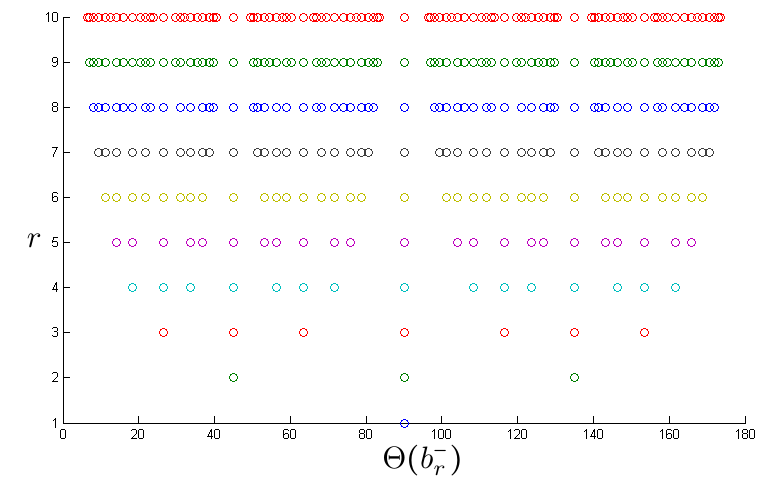
(Appendix F, Proposition 4). In other words, we have a 1-1 correspondence between (singleton) minimizers of $|{\bf y}\cdot{\bf g}^{\perp}|$ and the angular spectrum $\Theta(b^{-}_{r})$ . Moreover, it can be shown that if $\theta_{i}<\theta<\theta_{i+1}$ for some $\theta_{i},\theta_{i+1}\in\Theta(b^{-}_{r})$ , then either $\Psi=\{{\bf y}_{i}\}$ (for $\theta$ close to $\theta_{i}$ ) or $\Psi=\{{\bf y}_{i+1}\}$ (for $\theta$ close to $\theta_{i+1}$ ) or $\Psi=\{{\bf y}_{i},{\bf y}_{i+1}\}$ if $\theta=\theta_{i,i+1}$ , where $\theta_{i,i+1}\in(\theta_{i},\theta_{i+1})$ is a critical angle given by

\theta_{i,i+1}=\theta({\bf y}_{i}+{\bf y}_{i+1})\quad\mbox{ for }1\leq i\leq n-1.

For convenience, we also define $\theta_{0,1}=0$ and $\theta_{n,n+1}=\pi$ . Since one can also prove $\Psi=\{{\bf y}_{1}\}$ for $0:=\theta_{0,1}<\theta<\theta_{1}$ and $\Psi=\{{\bf y}_{n}\}$ for $\theta_{n}<\theta<\theta_{n,n+1}:=\pi$ , with this notation we have the general result

\Psi=\begin{cases}\{{\bf y}_{i}\}&\mbox{ if }\theta_{i}<\theta<\theta_{i,i+1}\quad\mbox{ for some }i=1,\ldots,n\\ \{{\bf y}_{i},{\bf y}_{i+1}\}&\mbox{ if }\theta=\theta_{i,i+1}\quad\mbox{ for some }i=1,\ldots,n-1\\ \{{\bf y}_{i+1}\}&\mbox{ if }\theta_{i,i+1}<\theta<\theta_{i+1}\quad\mbox{ for some }i=0,\ldots,n-1\\ \end{cases}

(Appendix F, Proposition 5 - note that we have carefully excluded $\theta_{0,1}:=0$ and $\theta_{n,n+1}=\pi$ from the middle case). In words, this means that the element(s) of $b^{-}_{r}$ closest to the line $L_{\bf g}$ are also the member(s) of $b^{-}_{r}$ that cast the shallowest angles with $L_{\bf g}$ from above and below. This statement is not true if $b^{-}_{r}$ is replaced with a generic subset of $\mathbb{Z}^{2}$ - see Figure 23. The remaining cases are $\theta=\theta_{i}\in\Theta(b^{-}_{r})$ and $\theta=0$ . We deal with the former first - in the first case we have

\Psi=\{{\bf y}\in b^{-}_{r}:\theta(y)=\theta_{i}\},

a set containing up to $r$ members, all of which are parallel to each other and to ${\bf g}$ . In order to make these ideas more concrete, Example 1 gives explicit expressions for $\Theta(b^{-}_{r})$ and $\Psi$ in the case $r=3$ . Also, in Appendix F Remark 19, we give an algorithm for computing $\Theta(b^{-}_{r})$ and $Y(b^{-}_{r}):=\{{\bf y}_{1},{\bf y}_{2},\ldots,{\bf y}_{n}\}$ for any $r$ .

Example 1

When $r=3$ we have

	$\displaystyle\Theta(b^{-}_{3})$	$\displaystyle:=$	$\displaystyle\{\theta_{1},\theta_{2},\theta_{3},\theta_{4},\theta_{5},\theta_{6},\theta_{7}\}$
		$\displaystyle=$	$\displaystyle\{\arctan(1/2),\frac{\pi}{4},\arctan(2),\frac{\pi}{2},\frac{\pi}{2}+\arctan(1/2),\frac{3\pi}{4},\frac{\pi}{2}+\arctan(2)\}.$

For $0<\theta\leq\frac{\pi}{2}$ , (we omit $\frac{\pi}{2}<\theta<\pi$ for brevity) the set of minimizers $\Psi$ is given by

\Psi=\begin{cases}\{(-2,-1)\}:=\{{\bf y}_{1}\}&\mbox{ if }0<\theta<\theta_{1,2}.\\ \{(-2,-1),(-1,-1)\}:=\{{\bf y}_{1},{\bf y}_{2}\}&\mbox{ if }\theta=\theta_{1,2}.\\ \{(-1,-1)\}:=\{{\bf y}_{2}\}&\mbox{ if }\theta_{1,2}<\theta<\theta_{2}.\\ \{(-1,-1),(-2,-2)\}:=\{{\bf y}_{2},2{\bf y}_{2}\}&\mbox{ if }\theta=\theta_{2}.\\ \{(-1,-1)\}:=\{{\bf y}_{2}\}&\mbox{ if }\theta_{2}<\theta<\theta_{2,3}.\\ \{(-1,-1),(-1,-2)\}:=\{{\bf y}_{2},{\bf y}_{3}\}&\mbox{ if }\theta=\theta_{2,3}.\\ \{(-1,-2)\}=\{{\bf y}_{3}\}&\mbox{ if }\theta_{2,3}<\theta<\theta_{3,4}.\\ \{(-1,-2),(0,-1)\}=\{{\bf y}_{3},{\bf y}_{4}\}&\mbox{ if }\theta=\theta_{3,4}.\\ \{(0,-1)\}:=\{{\bf y}_{4}\}&\mbox{ if }\theta_{3,4}<\theta<\theta_{4}.\\ \{(0,-1),(0,-2),(0,-3)\}:=\{{\bf y}_{4},2{\bf y}_{4},3{\bf y}_{4}\}&\mbox{ if }\theta=\theta_{4}.\end{cases}

where $\theta_{0,1}=0$ , $\theta_{1,2}=\arctan(2/3)$ , $\theta_{2,3}=\arctan(3/2)$ , $\theta_{3,4}=\arctan(3)$ .

When $\Psi$ is a singleton set, that is $\Psi=\{{\bf y}_{i}\}$ for some $1\leq i\leq n$ , (67) becomes ${\bf g}^{*}_{r}=\frac{{\bf y}_{i}}{\|{\bf y}_{i}\|}$ and we have

\theta({\bf g}^{*}_{r})=\theta\left(\frac{{\bf y}_{i}}{\|{\bf y}_{i}\|}\right)=\theta_{i}

On the other hand, if $\theta=\theta_{i}\in\Theta(b^{-}_{r})$ , ${\bf g}^{*}_{r}$ is a sum of vectors all parallel to one another and to ${\bf g}$ , and we get $\theta^{*}_{i}=\theta_{i}$ again. This is the lone case in which coherence transport doesn’t kink. Next, at the transition angles $\theta_{i,i+1}$ where $\Psi=\{{\bf y}_{i},{\bf y}_{i+1}\}$ , we have ${\bf g}^{*}_{r}=\frac{{\bf y}_{i}}{\|{\bf y}_{i}\|}+\frac{{\bf y}_{i+1}}{\|{\bf y}_{i+1}\|}$ , so that

\theta({\bf g}^{*}_{r})=\theta\left(\frac{{\bf y}_{i}}{\|{\bf y}_{i}\|}+\frac{{\bf y}_{i+1}}{\|{\bf y}_{i+1}\|}\right)=\frac{\theta_{i}+\theta_{i+1}}{2},

where we have used the observation (proved in Appendix F, Observation F.1) that $\theta({\bf v}+{\bf w})=\frac{\theta({\bf v})+\theta({\bf w})}{2}$ holds for all unit vectors ${\bf v},{\bf w}\in S^{1}$ . Finally, suppose $\theta=0$ . Here we have $\Psi=\{(i,-1):-r+1\leq i\leq r-1\}$ , giving

{\bf g}^{*}_{r}=e_{2}\qquad\mbox{for }\theta=0

after rescaling. In summary, for $\theta\in[0,\pi)$ we then have

\theta^{*}_{r}=\begin{cases}\frac{\pi}{2}&\mbox{ if }\theta=0\\ \theta_{i}&\mbox{ if }\theta_{i-1,i}<\theta<\theta_{i,i+1}\mbox{ for some }i=1,\ldots n\\ \frac{\theta_{i}+\theta_{i+1}}{2}&\mbox{ if }\theta=\theta_{i,i+1}\mbox{ for some }i=1,\ldots n\end{cases}

(68)

See Figure 21(a)-(b) for an illustration of (68) for $r=3$ and $r=5$ . In Appendix F, Corollary 2 we prove a generalization of this result that applies if, for example, the discrete ball used by coherence transport is replaced with a discrete square.

Remark 12

Since $\theta^{*}_{r}=\theta$ if and only if $\theta\in\Theta(b^{-}_{r})$ , and since the latter is generated by vectors with integer coordinates, it follows that for fixed $\theta=\arctan(x)$ , we have $\theta^{*}_{r}=\theta$ for all $r$ sufficiently large if $x$ is rational and $\theta^{*}_{r}\neq\theta$ for all $r$ if $x$ is irrational. In light of (57) and Theorem 7.2, this means that in the former case we have $u=u_{\mbox{m\"{a}rz}}$ for all $r$ sufficiently large, but in the latter case $\|u-u_{\mbox{m\"{a}rz}}\|_{p}\rightarrow 0$ for all $1\leq p<\infty$ , but we always have $u\neq u_{\mbox{m\"{a}rz}}$ for generic boundary data $u_{0}$ .

Guidefill. In this case (65) becomes

{\bf g}^{*}_{r,\mu}:=\sum_{{\bf y}\in\tilde{b}^{-}_{r}}e^{-\frac{\mu^{2}}{2r^{2}}({\bf y}\cdot{\bf g}^{\perp})^{2}}\frac{\bf y}{\|{\bf y}\|},

where $\tilde{b}^{-}_{r}$ is given by (26). It is useful to patition $\tilde{b}^{-}_{r}$ into a disjoint union of sets $\ell^{-}_{k}$ such at each $\ell^{-}_{k}$ is the collection of points in $\tilde{b}^{-}_{r}$ distance $k$ from the line $L_{\bf g}=\{\lambda{\bf g}:\lambda\in\mathbb{R}\}$ , that is

\ell^{-}_{k}=\{n{\bf g}+m{\bf g}^{\perp}\in\tilde{b}^{-}_{r}:m=\pm k\}.

Since the weights (6) exponentially decay with distance from $L_{\bf g}$ , then so long as $\ell^{-}_{0}$ is non-empty, we expect the contribution of the other $\ell^{-}_{k}$ to vanish. For Guidefill, $\ell^{-}_{0}$ can be explicitly parametrized as

	$\displaystyle\ell^{-}_{0}$	$\displaystyle:=$	$\displaystyle\{n{\bf g}\in\tilde{b}^{-}_{r}:n{\bf g}\cdot e_{2}\leq-1\}$
		$\displaystyle=$	$\displaystyle\{n{\bf g}:n=-r,\ldots,-\lceil\csc\theta\rceil\}.$

For $\ell^{-}_{0}$ to be non-empty, we need $\lceil\csc\theta\rceil\leq r$ , which occurs only if $\theta_{c}\leq\theta\leq\pi-\theta_{c}$ , where $\theta_{c}$ is the same critical angle (63) from Section 8.1.1. If $\ell^{-}_{0}\neq\emptyset$ , we have

$\displaystyle{\bf g}^{*}_{r,\mu}$	$\displaystyle=$	$\displaystyle\sum_{{\bf y}\in\ell^{-}_{0}}\frac{\bf y}{\\|{\bf y}\\|}+\sum_{k=1}^{r}\sum_{{\bf y}\in\ell^{-}_{k}}e^{-\frac{\mu^{2}}{2r^{2}}k^{2}\\|{\bf g}\\|^{2}}\frac{\bf y}{\\|{\bf y}\\|}$
	$\displaystyle\rightarrow$	$\displaystyle\sum_{{\bf y}\in\ell^{-}_{0}}\frac{\bf y}{\\|{\bf y}\\|}\qquad\mbox{ as }\mu\rightarrow\infty.$
	$\displaystyle=$	$\displaystyle\sum_{n=-r}^{-\lceil\csc\theta\rceil}n{\bf g}$
	$\displaystyle=$	$\displaystyle{\bf g}\qquad\mbox{ after rescaling. }$

Hence we transport in the correct direction in this case.

One the other hand, if $\ell^{-}_{0}=\emptyset$ but $\theta\neq 0$ , then the weights (6) concentrate all their mass into $\ell^{-}_{1}$ , with all other $\ell^{-}_{k}$ vanishing. Unfortunately, unlike $\ell^{0}$ , the set $\ell^{-}_{1}$ is not parallel to ${\bf g}$ so we expect kinking in this case. In general $\ell^{-}_{1}$ can consist of two parallel components on either side of $\ell^{-}_{0}$ . But in this case, since $\ell^{-}_{0}$ lies entirely above the line $y=-1$ , we know $\ell^{-}_{1}$ consists of just one component and we can write it explicitly as

\ell^{-}_{1}=\{n{\bf g}-\mbox{sgn}(\cos\theta){\bf g}^{\perp}:n=-r+1,\ldots,-1\}

(remember that ${\bf g}^{\perp}$ denotes the counterclockwise rotation of ${\bf g}$ by $90^{\circ}$ ). After rescaling by $e^{\frac{\mu^{2}}{2r^{2}}\|{\bf g}\|^{2}}$ we obtain

$\displaystyle{\bf g}^{*}_{r,\mu}$	$\displaystyle=$	$\displaystyle\sum_{{\bf y}\in\ell^{-}_{1}}\frac{\bf y}{\\|{\bf y}\\|}+\sum_{k=2}^{r}\sum_{{\bf y}\in\ell^{-}_{k}}e^{-\frac{\mu^{2}}{2r^{2}}(k^{2}-1)\\|{\bf g}\\|^{2}}\frac{\bf y}{\\|{\bf y}\\|}$
	$\displaystyle\rightarrow$	$\displaystyle\sum_{{\bf y}\in\ell^{-}_{1}}\frac{\bf y}{\\|{\bf y}\\|}\qquad\mbox{ as }\mu\rightarrow\infty.$
	$\displaystyle=$	$\displaystyle\left(\sum_{n=-r+1}^{-1}\frac{n}{\sqrt{1+n^{2}}}\right){\bf g}-\mbox{sgn}(\cos\theta)\left(\sum_{n=-r+1}^{-1}\frac{1}{\sqrt{1+n^{2}}}\right){\bf g}^{\perp}$
	$\displaystyle=$	$\displaystyle{\bf g}+\mbox{sgn}(\cos\theta)\alpha_{r}{\bf g}^{\perp}\qquad\mbox{ after rescaling. }$

where

\alpha_{r}=\frac{\sum_{n=1}^{r-1}\frac{1}{\sqrt{1+n^{2}}}}{\sum_{n=1}^{r-1}\frac{n}{\sqrt{1+n^{2}}}}.

Finally, if $\theta=0$ we have $\tilde{b}^{-}_{r}=b^{-}_{r}$ and we obtain ${\bf g}^{*}_{r}=e_{2}$ as for coherence transport. Defining $\Delta\theta_{r}=\arctan(\alpha_{r})$ , for $\theta\in[0,\pi)$ we obtain

\theta^{*}_{r}=\begin{cases}\frac{\pi}{2}&\mbox{ if }\theta=0\\ \theta+\Delta\theta_{r}&\mbox{ if }0<\theta<\theta_{c}\\ \theta&\mbox{ if }\theta_{c}\leq\theta\leq\pi-\theta_{c}\\ \theta-\Delta\theta_{r}&\mbox{ if }\pi-\theta_{c}<\theta<\pi.\end{cases}

(69)

In other words, aside from exceptional case $\theta=0$ , we have $\theta_{r}^{*}=\theta$ for the “well behaved” range of values $\theta_{c}\leq\theta\leq\pi-\theta_{c}$ , but $\theta_{r}^{*}$ jumps by a constant angle $\Delta\theta_{r}$ near $\theta=0$ and $\theta=\pi$ . The first few values of $\Delta\theta_{r}$ are $\Delta\theta_{3}\approx 35.8^{\circ}$ , $\Delta\theta_{4}\approx 30.0^{\circ}$ , $\Delta\theta_{5}\approx 25.9^{\circ}$ . See Figure 21(c)-(d) for an illustration of (69) for $r=3$ and $r=5$ .

Remark 13

Since $\theta_{c}=\arcsin(1/r)\rightarrow 0$ as $r\rightarrow\infty$ , it follows that for each fixed $\theta\in(0,\pi)$ we have $\theta^{*}_{r}=\theta$ and hence $u=u_{\mbox{m\"{a}rz}}$ for all $r$ sufficiently large. On the other hand, since $\theta_{c}>0$ , $\alpha_{r}>0$ for all $r$ , we never have $\theta^{*}_{r}=\theta$ independent of $\theta$ for any fixed $r$ . There are always angles we can’t reach.

Semi-implicit Guidefill. The analysis of semi-implicit Guidefill is the same as for Guidefill except that the set $\tilde{b}^{-}_{r}$ is replaced by $\tilde{b}^{0}_{r}$ . Defining $\ell^{0}_{k}$ as the collection of points in $\tilde{b}^{0}_{r}$ distance $k$ from the line $L_{\bf g}=\{\lambda{\bf g}:\lambda\in\mathbb{R}\}$ as before, we find that in this case

\ell^{0}_{0}:=\{n{\bf g}\in\tilde{b}_{r}:n{\bf g}\cdot e_{2}\leq 0\}

is never empty. In fact, for $0\leq\theta<\pi$ we have

\ell^{0}_{0}=\begin{cases}\{n{\bf g}:-r\leq n\leq-1\}&\mbox{ if }0<\theta<\pi\\ \{n{\bf g}:-r\leq n\leq r,n\neq 0\}&\mbox{ if }\theta=0.\end{cases}

If $\theta>0$ , we proceed as before and find

$\displaystyle{\bf g}^{*}_{r,\mu}$	$\displaystyle=$	$\displaystyle\sum_{{\bf y}\in\ell^{0}_{0}}\frac{\bf y}{\\|{\bf y}\\|}+\sum_{k=1}^{r}\sum_{{\bf y}\in\ell^{0}_{k}}e^{-\frac{\mu^{2}}{2r^{2}}k^{2}\\|{\bf g}\\|^{2}}\frac{\bf y}{\\|{\bf y}\\|}$
	$\displaystyle\rightarrow$	$\displaystyle\sum_{{\bf y}\in\ell^{0}_{0}}\frac{\bf y}{\\|{\bf y}\\|}\qquad\mbox{ as }\mu\rightarrow\infty.$
	$\displaystyle=$	$\displaystyle\sum_{n=-r}^{-1}n{\bf g}$
	$\displaystyle=$	$\displaystyle{\bf g}\qquad\mbox{ after rescaling. }$

However, if $\theta=0$ , this argument doesn’t work because the elements of $\ell^{0}_{0}$ all cancel each other out. In fact, in this case we have

{\bf g}^{*}_{r,\mu}=\underbrace{\sum_{{\bf y}\in\ell^{0}_{0}}\frac{\bf y}{\|{\bf y}\|}}_{=0}+\underbrace{\sum_{{\bf y}\in b^{-}_{r}}e^{-\frac{\mu^{2}}{2r^{2}}({\bf y}\cdot{\bf g}^{\perp})^{2}}\frac{\bf y}{\|{\bf y}\|}}_{\text{the ${\bf g}^{*}_{r,\mu}$ from coherence transport.}}.

Hence, in this case ${\bf g}^{*}_{r}=e_{2}$ yet again, just like for Guidefill and coherence transport. In general, for $0\leq\theta<\pi$ , we have

\theta^{*}_{r}=\begin{cases}\frac{\pi}{2}&\mbox{ if }\theta=0\\ \theta&\mbox{ if }0<\theta<\pi\end{cases}

(70)

In other words, semi-implicit Guidefill kinks only if ${\bf g}$ is exactly parallel to boundary of the inpainting domain. See Figure 21(e)-(f) for an illustration of (70) for $r=3$ and $r=5$ (the curves are of course the same, since (70) is independent of $r$ ).

Remark 14

In contrast to Guidefill and coherence transport, (70) tells us that for semi-implicit Guidefill in the limit $\mu\rightarrow\infty$ we have $\theta^{*}_{r}=\theta$ for all $\theta\in(0,\pi)$ , independent of $r$ . This is in fact exactly the same prediction (57) (albeit under stronger simplifying assumptions) that März and Bornemann obtained for coherence transport in their own continuum limit $u_{\mbox{m\"{a}rz}}$ as $\mu\rightarrow\infty$ (57). So in this case we have $u=u_{\mbox{m\"{a}rz}}$ independent of $r$ . We have in some sense come full circle - the original predictions of [6] for coherence transport under their high resolution and vanishing viscosity limit are the same as ours for semi-implicit Guidefill under our fixed ratio limit.

8.2 Asymptotic limit and blur

In this section we utilize the connection between Algorithm 1 and stopped random walks to explore the origins of blur artifacts. The main idea is that the continuum limit studied in Theorem 6.1 - while useful for studying kinking artifacts - is inadequate for studying blur. For the latter, one instead needs to consider an asymptotic limit where $h$ is very small but still non-zero. This is accomplished by leveraging a central limit theorem for the type of stopped random walk relevant to us, which states that our stopped random walk (or more precisely, its x-coordinate) is converging in distribution to a Gaussian as $h\rightarrow 0$ . Since we have the identity

u_{h}({\bf x})=\sum_{{\bf y}\in\mathcal{U}_{h}}\rho_{{\bf X}_{\tau}}({\bf y})u_{0}({\bf y}),

(71)

this suggests that $u_{h}$ can be related to a mollified version of $u_{0}$ , with a Gaussian mollifier. This idea is made precise in Conjecture 1, and is supported by numerical experiments (Figures 24 and 26). However, because the central limit theorem we utilize gives no rates of convergence, Conjecture 1 remains a conjecture - its rigorous proof will be the subject of future work. Before elaborating on these ideas, we first provide some motivation with a closer look at our $L^{p}$ convergence rates from Theorem 6.1, and a case in which they can be tightened - what we call degenerate stencils. If Conjecture 1 is true, then degenerate stencils give a sufficient condition under which blur artifacts can be avoided. However, they also tend to increase kinking artifacts, so there is an apparent trade-off (recall from Figure 6 that coherence transport kinks but doesn’t blur, while Guidefill blurs but doesn’t kink).

8.2.1 Degerate stencils and $L^{p}$ convergence rates

The first clue that blur artifacts might be present in $u_{h}$ comes from Theorem 6.1, where we see convergence to $u$ in $L^{p}$ for every $p\in[1,\infty)$ but not necessarily in $L^{\infty}$ . This is consistent with blur that is present for every $h>0$ but becomes less and less pronounced as $h\rightarrow 0$ . A clue that these artifacts might be in some cases be avoidable comes from the fact that if the stencil weights put all of their mass into a single ${\bf y}\in a^{*}_{r}$ (we call such weights degenerate), as occurs in coherence transport with ${\bf g}=(\cos\theta,\sin\theta)$ for all but finitely many $\theta$ (Section 8.1.2), then the bounds in Theorem 6.1 can be tightened. This is because the random walk ${\bf X}_{\tau}$ has become deterministic. All terms related to variances or probabilities are killed off, and the bound immediately changes to

\|u-u_{h}\|_{p}\leq K(rh)^{s\wedge\left(s^{\prime}+\frac{1}{p}\right)\wedge 1}.

(72)

In some cases, dependent on the boundary data $u_{0}:\mathcal{U}_{h}\rightarrow\mathbb{R}^{d}$ , it is even possible to prove convergence in $L^{\infty}$ for $u_{0}$ with jump discontinuities.

8.2.2 An asymptotic limit for Algorithm 1

The ideas in this section rely on the book [20], which covers the asymptotic distribution functions of certain stopped random walks. Recall that we have the identity (71), where $\rho_{{\bf X}_{\tau}}$ is the probability density function of the stopped random walk ${\bf X}_{\tau}={\bf x}+h\sum_{i=1}^{j}{\bf Z}_{i}$ . The steps $\{{\bf Z}_{i}\}=\{(V_{i},W_{i})\}$ are i.i.d. and take values in $\mbox{Supp}(a^{*}_{r})\subseteq\bar{b}^{-}_{r}$ (if we use the direct version of Algorithm 1) or $\mbox{Supp}(a^{*}_{r})\subseteq\bar{b}^{0}_{r}$ (if we use the semi-implicit extension) with probability density

P({\bf Z}_{i}={\bf y})=\frac{\tilde{w}_{r}({\bf 0},{\bf y})}{W},

(73)

where $\tilde{w}_{r}$ are the equivalent weights defined in Section 4. Denote the mean of ${\bf Z}_{i}:=(V_{i},W_{i})$ by $(\mu_{x},\mu_{y})$ and let $\tau$ given by (44) be the first passage time through $y=0$ . The bound $\mu_{y}<0$ is guaranteed (otherwise, the transport equation (34) is not well posed), and hence ${\bf X}_{\tau}$ has negative drift in the $y$ -direction. As we have already stated in Section 6.3, this type of random walk is well understood (20, Chapter 4), [21], [18], [19]. The way to understand blur artifacts is to recognize that $\rho_{{\bf X}_{\tau}}$ is a mollifier of sorts and moreover, because these types of stopped random walks obey a central limit theorem (20, Chapter 4, Theorem 2.3), $\rho_{{\bf X}_{\tau}}$ is converging in distribution to a Gaussian mollifier. In fact, if Conjecture 1 is correct, then the precise form of mollification is identical to the definition of discrete mollifaction presented in applications such as (28, Section 3), in the context of stabilizing noisy data for the purposes of numerical differentiation, and in [4] for more general applications. The mollifier is also equivalent to the one proposed in (28, Section 2).

Conjecture 1

Let the inpainting domain $D$ and undamaged area $\mathcal{U}$ , as well as their discrete counterparts $D_{h}$ , $\mathcal{U}_{h}$ be as described in Section 6.1. Let $u_{0}:\mathcal{U}\rightarrow\mathbb{R}^{d}$ denote as usual the undamaged portion of the image, and assume $u_{0}$ is non-negative and bounded, that is, there is an $M>0$ such that $0\leq u_{0}\leq M$ on $\mathcal{U}$ . Suppose we inpaint $D_{h}$ using Algorithm 1 or its semi-implicit extension, and denote the result by $u_{h}:D_{h}\rightarrow\mathbb{R}^{d}$ . Assume the assumptions of Section 6.1 hold and let $a^{*}_{r}$ denote the stencil of our inpainting method. Let ${Z_{i}}=(V_{i},W_{i})$ taking values in $\mbox{Supp}(a^{*}_{r})$ with mean $(\mu_{x},\mu_{y})$ denote the increments of the random walk described above, with probability density given by (73). Let $\Pi_{\theta^{*}_{r}}:D\rightarrow\partial D$ denote the transport operator defined in (36) (recall that that the transport direction ${\bf g}^{*}_{r}$ obeys ${\bf g}^{*}_{r}=(\mu_{x},\mu_{y})$ ). Then, if $u_{0}:\mathcal{U}\rightarrow\mathbb{R}^{d}$ is independent of its $y$ -coordinate, we have

u_{h}(x,y)\rightarrow(u_{0}\Big|_{y=0}*g_{\sigma(h)})(\Pi_{\theta^{*}_{r}}(x,y))\qquad\mbox{ asymptotically as }h\rightarrow 0

(74)

at a rate that is dependent on $y$ but independent of $x$ , where $u_{0}\Big|_{y=0}*g_{\sigma(h)}$ denotes the discrete mollification of $u_{0}\Big|_{y=0}$ with mollifier $g_{\sigma(h)}$ defined for any $x\in(0,1]$ by

\left(u_{0}\Big|_{y=0}*g_{\sigma(h)}\right)(x):=\sum_{i=1}^{N}\left[\int_{(i-1)h}^{ih}g_{\sigma(h)}(x-t)dt\right]u_{0}\Big|_{y=0}(ih).

and where $g_{\sigma(h)}$ is a one dimensional Gaussian kernel with $h$ -dependent variance given by

\sigma(h)^{2}=\frac{\gamma^{2}yh}{|\mu_{y}|^{3}}\quad\mbox{ where }\gamma^{2}=\operatorname{Var}(\mu_{x}W_{1}-\mu_{y}V_{1})

(75)

Moreover, for general $u_{0}$ we have

u_{h}(x,y)\rightarrow(\tilde{u}_{0}*g_{\sigma(h)})(\Pi_{\theta^{*}_{r}}(x,y))\qquad\mbox{ asymptotically as }h\rightarrow 0,

(76)

(again, at a rate dependent on $y$ but independent of $x$ ) where $\tilde{u}_{0}:\partial D_{h}\rightarrow\mathbb{R}^{d}$ obeys $\tilde{u}_{0}(ih)=\sum_{j=-r-1}^{0}\alpha_{j}(x)u_{0}(ih,jh)$ where for each $(ih,0)\in\partial D_{h}$ we have $0\leq\alpha_{j}(ih)\leq 1$ and $\sum_{j=-r-1}^{0}\alpha_{j}(ih)=1$ (in other words, for each $ih$ , $\tilde{u}_{0}(ih)$ is a convex combination of $u_{0}(ih,0)$ and the $r+1$ pixels directly below it).

Proof Idea: Although proving this conjecture is beyond the scope of our current work, we briefly sketch how a proof might go and where the technical challenges arise. First, note that it suffices to prove claim two, as the first claim is then a special case. Our first job is to define $\tilde{u}_{0}$ . To that end, note that

	$\displaystyle u_{h}(x,y)$	$\displaystyle=$	$\displaystyle\sum_{i=1}^{N}\sum_{j=-r-1}^{0}\rho_{{\bf X}_{\tau}}(ih,jh)u_{0}(ih,jh)$
		$\displaystyle=$	$\displaystyle\sum_{i=1}^{N}\rho_{X_{\tau}}(ih)\underbrace{\sum_{j=-r-1}^{0}\rho_{Y_{\tau}\|X_{\tau}}(jh\|ih)u_{0}(ih,jh)}_{:=\tilde{u}_{0}(ih)}.$

This definition of $\tilde{u}_{0}$ obeys the claimed properties since $\alpha_{j}(ih):=\rho_{Y_{\tau}|X_{\tau}}(jh|ih)$ obeys $0\leq\alpha_{j}(ih)\leq 1$ and $\sum_{j=-r-2}^{0}\alpha_{j}(ih)=1$ for all $i=1,\ldots N$ as claimed. Next, define $\hat{x}(x,y):=\Pi_{\theta^{*}_{r}}(x,y)$ for convenience. Fix $y>0$ and let $\epsilon>0$ . Our goal is to show that for $h$ sufficiently small we have

|u_{h}(x,y)-(\tilde{u}_{0}*g_{\sigma(h)})(\hat{x}(x,y))|<\epsilon

independent of $x$ . To that end, note that

|u_{h}(x,y)-(\tilde{u}_{0}*g_{\sigma(h)})(\hat{x}(x,y))|=\left|\sum_{i=1}^{N}\tilde{u}_{0}(ih)\left[\rho_{X_{\tau}}(ih)-\int_{(i-1)h}^{ih}g_{\sigma(h)}(\hat{x}-t)dt\right]\right|.\\

It follows from (20, Chapter 4, Theorem 2.3) that

\rho_{X_{\tau}}(ih)\rightarrow\int_{(i-1)h}^{ih}g_{\sigma(h)}(\hat{x}-t)dt

as $h\rightarrow 0$ . However, since the number of terms in the above sum is also diverging to infinity as $h\rightarrow 0$ , a convergence rate is needed to quantify the balance between these competing effects. Unfortunately, none are given. In the future, we hope to derive rates ourselves, so that we can upgrade Conjecture 1 to a theorem.

Remark 15

Conjecture 1 says that $u_{h}(x,y)$ , which we already know from Theorem 6.1 convergences as $h\rightarrow 0$ to the solution of the transport equation (34), can also be viewed asymptotically for small but non-zero $h$ as a solution to the same transport equation but where the boundary data has been mollified by a Gaussian kernel $g_{\sigma(h)}$ . Moreover, the degree of mollification (75) increases as we move further into the inpainting domain (that is, $\sigma(h)$ increases) and decreases as $h\rightarrow 0$ ( $\sigma(h)$ decreases). In fact, we have already observed in Figure 18 that $g_{\sigma(h)}$ is converging as $h\rightarrow 0$ to a Dirac delta distribution.

8.2.3 Angular dependence of blur artifacts

Conjecture 1 proposes an asymptotic relationship between $u_{h}(x,y)$ and the convolution of $u_{0}(x,0)$ with a Gaussian kernel of $h$ -dependent variance $\sigma(h)^{2}$ given by (75). Although currently only a conjecture and valid only valid asymptotically as $h\rightarrow 0$ , Figures 24 and 26 suggest that the conjecture is not only valid but gives an extremely good approximation even for very small images (The example in Figure 24 is only $200\times 200$ px). Conjecture 1 has three takeaway messages:

•

Blur gets worse as one moves further into the inpainting domain and (e.g. $y$ increases) - Figures 24 and 26.
•

Blur gets better as $h\rightarrow 0$ - Figure 25.
•

Blur is non-existent if the stencil weights are degenerate - that is, put all of their mass into a single real pixel ${\bf y}$ (since in this case ${\bf Z}_{i}$ is deterministic and all variances are $0$ ).

All three of these observations are consistent with experience. The third point in particular explains why coherence transport, which has a degenerate stencil in the limit $\mu\rightarrow\infty$ for all but finitely many $\theta=\theta({\bf g})$ (Section 8.1.2), does not appear to suffer from blur artifacts at all, e.g. Figure 6. However, it also predicts that for those few special angles where coherence transport puts its mass into more than one ${\bf y}\in b^{-}_{r}$ , it will blur just like everything else (experiments, which we omit for the sake of space, confirm this).

What is less clear from (75) is how $\sigma(h)^{2}$ depends on ${\bf g}=(\cos\theta,\sin\theta)$ , as $\frac{\gamma^{2}}{|\mu_{y}^{3}|}$ can be quite complex in general (certainly for semi-implicit Guidefill at least, where $|\mu_{y}|=g^{*}_{r}\cdot e_{2}$ can get arbitrarily close to $0$ , we expect severe blur artifacts for shallow angles). Figure 27 illustrates the angular dependence of $\sigma(h)$ as a function of $\theta\in[0,\pi]$ with $y=1$ and $h=0.01$ fixed, for the three main methods of interest - coherence transport, Guidefill, and semi-implicit Guidefill (note the log scale). In every case we have $r=3$ and $\mu=100$ .

Remark 16

Figure 27 suggests a trade-off of sorts between kinking artifacts and blur artifacts. If Conjecture 1 is true, then semi-implicit Guidefill, the only method considered so far capable of avoiding kinking artifacts unless ${\bf g}=(\cos\theta,\sin\theta)$ is exactly parallel to the inpainting domain, that is ${\bf g}^{*}_{r}={\bf g}$ unless $\theta\in\{0,\pi\}$ , pays a price for this ability with blurring artifacts that become arbitrarily bad as $\theta\rightarrow 0$ or $\theta\rightarrow\pi$ . At the opposite extreme, coherence transport suffers from no blur at all for all but finitely many angles, but also kinks (that is ${\bf g}^{*}_{r}\neq{\bf g}$ ) for all but finitely many angles (Figure 5). Guidefill is in the middle: ${\bf g}^{*}_{r}={\bf g}$ so long as $\theta$ is not too shallow, and blur exists but remains bounded. It remains to be seen whether a method be completely free of both kinking and blur artifacts, but it seems unlikely. A more modest goal would be to design a method which like semi-implicit Guidefill suffers from no kinking artifacts, but for which $\sigma(h)$ defined by (75) remains bounded for all $\theta$ , like Guidefill. Whether or not this is possible also remains to be seen, and is something we would like to investigate in the future.

9 Numerical Experiments

In this section we have three objectives:

1.

To compare the limiting transport directions derived in Section 8.1.2 for coherence transport, Guidefill, and semi-implicit Guidefill as $\mu\rightarrow\infty$ with the orientation of extrapolated isophotes when the algorithm is run in practice.
2.

To check experimentally our claim in Section 7.1 that when $r$ is a small integer, our limit $u$ typically does a better job of capturing the behaviour of $u_{h}$ than $u_{\mbox{m\"{a}rz}}$ does, that is $\|u_{h}-u\|_{p}\ll\|u_{h}-u_{\mbox{m\"{a}rz}}\|_{p}$ .
3.

To verify our bounds in Theorem 6.1 and check that they are tight. Further, we wish to see whether or not our results continue to hold if some of our simplifying assumptions are relaxed (specifically, Guidefill with a constant guidance direction ${\bf g}$ replaced by a smoothly varying transport field ${\bf g}({\bf x})$ ).

We will perform one experiment for each objective, but for the sake of space, Experiment III is deferred to Appendix H. For Experiments II and III, we will experiment using a variety of boundary data $u_{0}$ satisfying the hypotheses of Section 6.3, as well as a few different inpainting methods that are each special cases of Algorithm 1. These are presented in detail in Appendix G.

9.1 Experiment I: Validation of limiting transport directions for coherence transport, Guidefill, and semi-implicit Guidefill.

In this experiment we compare the limiting transport directions derived in Section 8.1.2 for coherence transport, Guidefill, and semi-implicit Guidefill as $\mu\rightarrow\infty$ with the orientation of extrapolated isophotes in an actual inpainted image $u_{h}$ obtained in practice with finite $\mu$ . In each case we choose as our boundary data the image shown in Figure 28(a), consisting of a red dot on a blue background, with the inpainting domain shown in yellow. We run each algorithm with

{\bf g}=(\cos(k^{\circ}),\sin(k^{\circ}))

for $k=0,1,\ldots,90$ , with $\mu=40$ fixed and for various values of $r$ . The dot is then stretched into a line as in Figure 28(b), the orientation of which gives ${\bf g}^{*}_{\mu,r}$ and which can be measured numerically.

Results are shown in Figure 29 for $r=3$ and $r=5$ . The top row (a)-(c) gives the theoretical curves for $r=3$ , with the actual measured results in the row underneath (d)-(f). The third row (g)-(i) gives the theoretical curves for $r=5$ , while the final row (j)-(l) gives corresponding real measurements. While we see some smoothing out of the jump discontinuities in the case of coherence transport, this is expected as one can easily show that the convergence to $\theta^{*}=\lim_{\mu\rightarrow\infty}\theta^{*}_{r,\mu}$ is pointwise but not uniform, becoming arbitrarily slow in the vicinity of the jumps. On the other hand, for Guidefill and semi-implicit Guidefill we see excellent agreement with theory even in the vicinity of jump discontinuities. This is to be expected as well, since one can easily show that the relevant limits are uniform in this case.

9.1.1 Experiment II: Comparison of convergence rates to both continuum limits

Our second experiment explores the relationship between $\|u_{h}-u\|_{p}$ and
$\|u_{h}-u_{\mbox{m\"{a}rz}}\|_{p}$ , for $u_{h}$ such that the limit $u_{\mbox{m\"{a}rz}}$ exists, and under the assumption that we are not in the trivial case $u=u_{\mbox{m\"{a}rz}}$ . From Section 7.1 we have the bound

\|u-u_{\mbox{m\"{a}rz}}\|_{p}\leq K_{1}\cdot(rh)^{(\frac{s^{\prime}}{2}+\frac{1}{2p})\wedge\frac{s}{2}\wedge 1}+K_{2}r^{-q\left\{s\wedge\left(s^{\prime}+\frac{1}{p}\right)\wedge 1\right\}}.

(77)

If this bound is tight, then when $r$ is a small integer and $h$ is small, we expect $\|u_{h}-u\|_{p}\ll\|u_{h}-u_{\mbox{m\"{a}rz}}\|_{p}$ . At the same time, Theorem 7.2 shows that $u\rightarrow u_{\mbox{m\"{a}rz}}$ as $r\rightarrow\infty$ , so we expect $\|u_{h}-u\|_{p}\approx\|u_{h}-u_{\mbox{m\"{a}rz}}\|_{p}$ when $r$ is large. Figure 30 tests this by plotting $\|u_{h}-u\|_{p}$ and $\|u_{h}-u_{\mbox{m\"{a}rz}}\|_{p}$ as a function of $r$ with $h$ fixed and for various choices of $p$ , and for a few choices of boundary data $u_{0}$ and inpainting methods from Appendix G. Specifically, the boundary data $u_{0}$ is given by (85) for various values of $s$ and $s^{\prime}$ , and the weights and neighborhoods are as in Example 1 and Example 2 from Appendix G. The results confirm our expectations. For the sake of space, we only show a few illustrative examples.

10 Conclusions and Future Work

In this paper we have presented a detailed analysis of a class of geometric inpainting algorithms based on the idea of filling the inpainting domain in successive shells from the boundary inwards, where every pixel to be filled is assigned a color equal to a weighted average of its already filled neighbors. These methods are all special cases of a generic framework sketched in Algorithm 1. Methods in the literature falling within this framework include

•

Telea’s Algorithm [32].
•

Coherence Transport [6, 25].
•

Guidefill [23].

A subtle but important point about these methods is that pixels in the current inpainting boundary are filled independently. Noting this, we have proposed a semi-implicit extension of these methods in which pixels in the current shell are instead filled simultaneously by solving a linear system. We have also sketched in Algorithm 1 a straightforward extension of the original framework that is equivalent to solving this linear system using damped Jacobi or successive over-relaxation (SOR). A theoretical convergence analysis of these methods is presented for the semi-implicit extension of Guidefill, where we show that SOR is extremely effective. This analysis is backed up by numerical experiments. We also present in some detail additional features of semi-implicit Guidefill relating to how the method decides on a good order to fill pixels, but this is not the main focus of our work.

As all of the algorithms listed above (with the exception of semi-implicit Guidefill, which is presented for the first time in this paper) are known to create some disturbing visual artifacts, the main objective of our analysis is to understand why these occur and whether or not they are inevitable. We focus specifically on kinking artifacts and blur artifacts. Other artifacts including the formation of shocks and extrapolated isophotes that end abruptly are discussed but not analyzed, as they have already been studied elsewhere [6, 26] and are well understood. Our analysis is based on two key ideas:

•

A continuum limit, which we use to explain kinking artifacts.
•

A connection to the theory of stopped random walks, which we use both to prove convergence to our continuum limit, and to explore blur artifacts.

Similarly to the earlier work of Bornemann and März [6], our continuum limit is a transport equation. However, our limit process is different and so are the coefficients of the resulting transport equation. Moreover, numerical experiments show that our transport equation is a better reflection of the behaviour of Algorithm 1 (the direct form and our proposed semi-implicit extension) in practice, capable of accurately predicting kinking phenomena that is not captured by the alternative continuum limit proposed in [6]. The second core idea of our analysis, which is to relate Algorithm 1 and its extension to stopped random walks, is critical for two reasons. Firstly, it allows us to prove convergence to our continuum limit even for boundary data with low regularity, such as (finitely many) jump discontinuities. By contrast, the analysis in [6] assumes smooth boundary data, which is an unrealistic assumption for images. Secondly, this connection is central to our analysis of blur artifacts, which we analyze based not on a continuum limit where $h\rightarrow 0$ , but rather an asymptotic limit where $h$ very small but nonzero. While we have not (yet) been able to prove convergence to this asymptotic limit, it allows us to make quantitative predictions that are in excellent agreement with numerical experiments, even for relatively low resolution images (e.g. Figure 24 which is only $200\times 200$ px). Our analysis operates in a highly idealized setting (Section 6.1), but our conclusions are far reaching. In particular, we prove the following:

1.

The rate of convergence to our continuum limit depends on the regularity of the boundary data, and convergence is slower for boundary data with lower regularity. Thus, our continuum limit $u$ does a better job of approximating the actual inpainted image $u_{h}$ when the boundary data $u_{0}$ is smooth (Theorem 6.1).
2.

The difference between our continuum limit and the one proposed in [6] is most significant when the radius $r$ of the averaging neighborhood $A_{\epsilon,h}({\bf x})$ (measured in pixels) is small, and goes to zero as $r\rightarrow\infty$ (Theorem 7.2).
3.

In the direct form of Algorithm 1, kinking artifacts will always be present. That is, certain isophotes cannot be extended into the inpainting domain without bending (Section 8.1.1).
4.

This is not true of the semi-implicit extension of Algorithm 1. In particular, semi-implicit Guidefill can extrapolate isophotes with any orientation²² 2 that is, unless the isophotes are exactly parallel to the boundary of the inpainting domain. But in this case extrapolation is not defined., and moreover is able to do so efficiently by using SOR to solve the required linear system (Section 8.1.1, Section 8.1.2, Corollary 1).

The following results, which we do not prove, are implied by Conjecture 1 if it is true:

1.

Blur artifacts exhibit an angular dependence, which for semi-implicit Guidefill becomes arbitrarily bad as the angle an extrapolated isophote makes with the boundary of the inpainting domain goes to zero. Thus, semi-implicit Guidefill pays a heavy price (on top of the need to solve a linear system for every shell) for its ability to successfully extrapolate such isophotes (Conjecture 1, Figure 27).
2.

Blur artifacts become less significant as the resolution of the image goes up, and get worse the further into the inpainting domain you extrapolate (Conjecture 1).
3.

Methods that put all of their weight into a single pixel exhibit no blur, but can only extrapolate without kinking in finitely many directions (Remark 16).

The last of these conclusions suggest that there is an apparent trade off between kinking artifacts and blur artifacts, however, this is something that requires additional investigation. Our inability to prove Conjecture 1 is due to a result on stopped random walks from [20] - that our result depends on - failing to give rates of convergence. In the future we hope to derive those rates ourselves so that we can prove or disprove this conjecture. In fact, there are a number of questions we would like to explore in the future.

1.

Does there exist an algorithm within the framework we have described that avoids blurring artifacts and kinking artifacts at the same time? If not, is it at least possible to design an algorithm that, like semi-implicit Guidefill, avoids kinking artifacts so long as the guidance direction ${\bf g}=(\cos\theta,\sin\theta)$ obyes $\theta\neq 0$ , but for which the severity of blur as a function of $\theta$ remains bounded? Could this be done, for example, by the replacing the bilinear interpolation used to define ghost pixels with a more sophisticated interpolation scheme?
2.

While we have already shown that SOR (with appropriate ordering of unknowns) is particularly effective for solving the linear system arising in semi-implicit Guidefill, is this generically true regarding the semi-implicit extension of any inpainting method within the class under investigation? Moreover, SOR is not ideal because it is sequential whereas Guidefill was designed to be a parallel algorithm. Does another method exist which maintains the fast convergence rate of SOR, but can be implemented in parallel? One possibility here is the scheduled Jacobi method [1].
3.

Is our semi-implicit extension of Algorithm 1 the best way of avoiding kinking artifacts? In our analysis, we have assumed that the radius of our averaging neighborhood remains fixed. Another possibility, based on the observation that as $r$ increases, (direct) Guidefill is able to successfully extrapolate shallower and shallower angles (Section 8.1.2), is to use the direct form of Guidefill but dynamically resize $\tilde{B}_{\epsilon,h}({\bf x})$ as needed.
4.

What happens if the semi-implicit version of Algorithm 1 is generalized to a fully-implicit extension in which pixel colors are computed as a weighted average not only of their (known) already filled neighbors in $A_{\epsilon,h}({\bf x})\cap\Omega\backslash D^{(k)}$ and (unknown) neighbors within the same shell $\partial D^{(k)}_{h}$ , but of all neighbors in $A_{\epsilon,h}({\bf x})$ ? Are their additional benefits in terms of artifact reduction and, if so, can the resulting linear system be solved efficiently enough to make this worthwhile?

11 Acknowledgements

The authors would like to thank Vittoria Silvestri, James Norris, and Arieh Iserles for helpful conversations. Thanks is also due to Dömötör Pálvölgyi, whose idea of a symmetry-based argument eventually led to Appendix F, Proposition 5.

References

(1) J. Adsuara, I. Cordero-Carrión, P. Cerdá-Durán, and M. Aloy, Scheduled relaxation jacobi method: Improvements and applications, Journal of Computational Physics, 321 (2016), pp. 369 – 413, doi:http://dx.doi.org/10.1016/j.jcp.2016.05.053, http://www.sciencedirect.com/science/article/pii/S002199911630198X.
(2) P. Arias, G. Facciolo, V. Caselles, and G. Sapiro, A variational framework for exemplar-based image inpainting, Int. J. Comput. Vision, 93 (2011), pp. 319–347, doi:10.1007/s11263-010-0418-7, http://dx.doi.org/10.1007/s11263-010-0418-7.
(3) C. Ballester, M. Bertalmio, V. Caselles, G. Sapiro, and J. Verdera, Filling-in by joint interpolation of vector fields and gray levels, IEEE Transactions on Image Processing, 10 (2001), pp. 1200–1211, doi:10.1109/83.935036.
(4) J. V. Beck, The mollification method and the numerical solution of ill-posed problems (diego a. murio), SIAM Review, 36 (1994), pp. 502–503, doi:10.1137/1036117, https://doi.org/10.1137/1036117, arXiv:https://doi.org/10.1137/1036117.
(5) M. Bertalmio, G. Sapiro, V. Caselles, and C. Ballester, Image inpainting, in Proceedings of the 27th annual conference on Computer graphics and interactive techniques, ACM Press/Addison-Wesley Publishing Co., 2000, pp. 417–424.
(6) F. Bornemann and T. März, Fast image inpainting based on coherence transport, Journal of Mathematical Imaging and Vision, 28 (2007), pp. 259–278, doi:10.1007/s10851-007-0017-6, http://dx.doi.org/10.1007/s10851-007-0017-6.
(7) M. Burger, L. He, and C. Schönlieb, Cahn-hilliard inpainting and a generalization for grayvalue images, SIAM J. Imaging Sci., 2 (2009), pp. 1129–1167.
(8) P. Buyssens, O. L. Meur, M. Daisy, D. Tschumperlé, and O. Lézoray, Depth-guided disocclusion inpainting of synthesized rgb-d images, IEEE Transactions on Image Processing, 26 (2017), pp. 525–538, doi:10.1109/TIP.2016.2619263.
(9) T. Chan, S. Kang, and J. Shen, Euler’s elastica and curvature-based inpainting, SIAM Journal on Applied Mathematics, (2002), pp. 564–592.
(10) T. Chan and J. Shen, Variational image inpainting, Communications on pure and applied mathematics, 58 (2005), pp. 579–619.
(11) J. Cilleruelo, The distribution of the lattice points on circles, Journal of Number Theory, 43 (1993), pp. 198 – 202, doi:http://dx.doi.org/10.1006/jnth.1993.1017, http://www.sciencedirect.com/science/article/pii/S0022314X83710176.
(12) A. Criminisi, P. Pérez, and K. Toyama, Region filling and object removal by exemplar-based image inpainting, IEEE Transactions on Image Processing, 13 (2004), pp. 1200–1212.
(13) I. Daribo and B. Pesquet-Popescu, Depth-aided image inpainting for novel view synthesis, in 2010 IEEE International Workshop on Multimedia Signal Processing, Oct 2010, pp. 167–170, doi:10.1109/MMSP.2010.5662013.
(14) V. Derr and D. Kinzebulatov, On the extension of schwartz distributions to the space of discontinuous test functions of several variables, Rocky Mountain J. Math., 39 (2009), pp. 1173–1193, doi:10.1216/RMJ-2009-39-4-1173, http://dx.doi.org/10.1216/RMJ-2009-39-4-1173.
(15) domotorp (http://mathoverflow.net/users/955/domotorp), Conjecture regarding closest point inside a discrete ball to a line. MathOverflow, http://mathoverflow.net/q/187830, arXiv:http://mathoverflow.net/q/187830. URL:http://mathoverflow.net/q/187830 (version: 2014-11-22).
(16) P. Erdös and R. Hall, On the angular distribution of gaussian integers with fixed norm, Discrete Mathematics, 200 (1999), pp. 87 – 94, doi:http://dx.doi.org/10.1016/S0012-365X(98)00329-X, http://www.sciencedirect.com/science/article/pii/S0012365X9800329X.
(17) C. Guillemot and O. L. Meur, Image inpainting : Overview and recent advances, IEEE Signal Processing Magazine, 31 (2014), pp. 127–144, doi:10.1109/MSP.2013.2273004.
(18) A. Gut, On the moments and limit distributions of some first passage times, Ann. Probab., 2 (1974), pp. 277–308, doi:10.1214/aop/1176996709, http://dx.doi.org/10.1214/aop/1176996709.
(19) A. Gut, On the moments of some first passage times for sums of dependent random variables, Stochastic Processes and their Applications, 2 (1974), pp. 115 – 126, doi:http://dx.doi.org/10.1016/0304-4149(74)90015-5, http://www.sciencedirect.com/science/article/pii/0304414974900155.
(20) A. Gut, Stopped Random Walks: Limit Theorems and Applications, Springer Series in Operations Research and Financial Engineering, Springer New York, 2009, https://books.google.co.uk/books?id=tWfBs5G7jHIC.
(21) A. Gut and S. Janson, The limiting behaviour of certain stopped sums and some applications, Scandinavian Journal of Statistics, 10 (1983), pp. 281–292, http://www.jstor.org/stable/4615930.
(22) G. H. Hardy, Weierstrass’s non-differentiable function, Transactions of the American Mathematical Society, 17 (1916), pp. 301–325, http://www.jstor.org/stable/1989005.
(23) L. R. Hocking, R. MacKenzie, and C.-B. Schönlieb, Guidefill: Gpu accelerated, artist guided geometric inpainting for 3d conversion of film, http://arxiv.org/abs/1611.05319.
(24) L. Ma, L. Do, and P. H. N. de With, Depth-guided inpainting algorithm for free-viewpoint video, in 2012 19th IEEE International Conference on Image Processing, Sept 2012, pp. 1721–1724, doi:10.1109/ICIP.2012.6467211.
(25) T. März, Image inpainting based on coherence transport with adapted distance functions, SIAM J. Img. Sci., 4 (2011), pp. 981–1000, doi:10.1137/100807296, http://dx.doi.org/10.1137/100807296.
(26) T. März, A well-posedness framework for inpainting based on coherence transport, Foundations of Computational Mathematics, 15 (2015), pp. 973–1033, doi:10.1007/s10208-014-9199-7, http://dx.doi.org/10.1007/s10208-014-9199-7.
(27) S. Masnou and J. Morel, Level lines based disocclusion, in Image Processing, 1998. ICIP 98. Proceedings. 1998 International Conference on, IEEE, 1998, pp. 259–263.
(28) D. Murio, C. Mejía, and S. Zhan, Discrete mollification and automatic numerical differentiation, Computers & Mathematics with Applications, 35 (1998), pp. 1 – 16, doi:http://dx.doi.org/10.1016/S0898-1221(98)00001-7, http://www.sciencedirect.com/science/article/pii/S0898122198000017.
(29) E. D. Nezza, G. Palatucci, and E. Valdinoci, Hitchhiker’s guide to the fractional sobolev spaces, Bulletin des Sciences Mathématiques, 136 (2012), pp. 521 – 573, doi:http://dx.doi.org/10.1016/j.bulsci.2011.12.004, http://www.sciencedirect.com/science/article/pii/S0007449711001254.
(30) R. Sadek, G. Facciolo, P. Arias, and V. Caselles, A variational model for gradient-based video editing, International Journal of Computer Vision, 103 (2013), pp. 127–162, doi:10.1007/s11263-012-0597-5, http://dx.doi.org/10.1007/s11263-012-0597-5.
(31) C.-B. Schönlieb, Partial Differential Equation Methods for Image Inpainting, 2015.
(32) A. Telea, An image inpainting technique based on the fast marching method, Journal of Graphics Tools, 9 (2004), pp. 23–34.
(33) D. TschumperlÉ, Fast anisotropic smoothing of multi-valued images using curvature-preserving pde’s, International Journal of Computer Vision, 68 (2006), pp. 65–82, doi:10.1007/s11263-006-5631-z, http://dx.doi.org/10.1007/s11263-006-5631-z.
(34) J. Varah, A lower bound for the smallest singular value of a matrix, Linear Algebra and its Applications, 11 (1975), pp. 3 – 5, doi:http://dx.doi.org/10.1016/0024-3795(75)90112-3, http://www.sciencedirect.com/science/article/pii/0024379575901123.
(35) R. Varga, Matrix iterative analysis, Prentice-Hall series in automatic computation, Prentice-Hall, 1962, https://books.google.co.uk/books?id=PFYWAAAAIAAJ.
(36) Y. Wexler, E. Shechtman, and M. Irani, Space-time completion of video, IEEE Trans. Pattern Anal. Mach. Intell., 29 (2007), pp. 463–476, doi:10.1109/TPAMI.2007.60.
(37) D. Williams, Probability with Martingales, Cambridge mathematical textbooks, Cambridge University Press, 1991, https://books.google.co.uk/books?id=RnOJeRpk0SEC.

Appendix A Punctured sums

Here we provide further justification for our exclusion of the point ${\bf x}$ from the update formula (1) in Algorithm 1 as mentioned in Remark 4. As we mentioned there, this makes no difference to the direct form of Algorithm 1, because the subroutine FillRow only involves sums taken over $A_{\epsilon,h}({\bf x})\cap(\Omega\backslash D^{(k)})$ , which never contains ${\bf x}$ . However, the semi-implicit extension of Algorithm 1 expresses $u_{h}({\bf x})$ as a sum of $u_{h}({\bf y})$ over a set of points that might include ${\bf x}$ . The reason we deliberately exclude ${\bf x}$ is because, as the following proposition shows, if $w_{\epsilon}({\bf x},{\bf x})<\infty$ , it doesn’t matter, but if $w_{\epsilon}({\bf x},{\bf x})=\infty$ , it wreaks havoc. Moreover, the weights (6) which we wish to study do have the property that $w_{\epsilon}({\bf x},{\bf x})=\infty$ .

Proposition 2

Suppose ${\bf x}\in B$ for some finite set $B\subset\mathbb{R}^{2}$ , and suppose there exist non negative weights $w:B\times B\rightarrow[0,\infty]$ , finite everywhere except possibly at $({\bf x},{\bf x})$ . Then if $w({\bf x},{\bf x})<\infty$ , we have

u_{h}({\bf x})=\frac{\sum_{{\bf y}\in B}w({\bf x},{\bf y})u_{h}({\bf y})}{\sum_{{\bf y}\in B}w({\bf x},{\bf y})}=\frac{\sum_{{\bf y}\in B\backslash\{{\bf x}\}}w({\bf x},{\bf y})u_{h}({\bf y})}{\sum_{{\bf y}\in B\backslash\{{\bf x}\}}w({\bf x},{\bf y})}.

On the other hand, if $w({\bf x},{\bf x})=\infty$ , we have an indeterminate expression

u_{h}({\bf x})=\frac{\infty}{\infty}.

Proof

The proof is an exercise in cancellation and left to the reader. ∎

Appendix B Properties of Ghost Pixels and Equivalent Weights

In this appendix we prove the six properties of ghost pixels and equivalent weights listed in Section 4. These properties all follow from the definition of $u_{h}({\bf y})$ when ${\bf y}$ is a ghost pixel, namely

u_{h}({\bf y})=\sum_{{\bf z}\in\mbox{Supp}(\{{\bf y}\})}\Lambda_{{\bf z},h}({\bf y})u_{h}({\bf z}),

where $\{\Lambda_{{\bf z},h}\}_{{\bf z}\in\mathbb{Z}^{2}_{h}}$ denote the basis functions of bilinear interpolation associated with the lattice $\mathbb{Z}^{2}_{h}$ , and where $\mbox{Supp}(A)$ denotes the set of real pixels needed to define a set $A$ of ghost pixels using bilinear interpolation. Note that if ${\bf y}\in A$ , then

\Lambda_{{\bf z},h}({\bf y})=0\quad\mbox{ for all }{\bf z}\notin\mbox{Supp}(A).

(78)

The following explicit formula for $\mbox{Supp}(\{(x,y)\})$ (which comes from the definition of bilinear interpolation) will occasionally be useful.

\mbox{Supp}(\{(x,y)\})=\left\{\left(\left\lfloor\frac{x}{h}\right\rfloor h,\left\lfloor\frac{y}{h}\right\rfloor h\right),\left(\left\lceil\frac{x}{h}\right\rceil h,\left\lfloor\frac{y}{h}\right\rfloor h\right),\left(\left\lfloor\frac{x}{h}\right\rfloor h,\left\lceil\frac{y}{h}\right\rceil h\right),\left(\left\lceil\frac{x}{h}\right\rceil h,\left\lceil\frac{y}{h}\right\rceil h\right)\right\}.

(79)

First we prove property one.

1. Explicit formula:

\tilde{w}({\bf x},{\bf z})=\sum_{{\bf y}\in A({\bf x})}\Lambda_{{\bf y},h}({\bf z})w({\bf x},{\bf y})

Proof

This follows straightforwardly from the definition of ghost pixels, the property (78), and a few exchanges of finite sums.

$\displaystyle u_{h}({\bf x})$	$\displaystyle=$	$\displaystyle\sum_{{\bf y}\in A({\bf x})}w({\bf x},{\bf y})u_{h}({\bf y})$
	$\displaystyle=$	$\displaystyle\sum_{{\bf y}\in A({\bf x})}w({\bf x},{\bf y})\sum_{{\bf z}\in\mbox{Supp}(\{{\bf y}\})}\Lambda_{{\bf z},h}({\bf y})u_{h}({\bf z})$
	$\displaystyle=$	$\displaystyle\sum_{{\bf y}\in A({\bf x})}w({\bf x},{\bf y})\sum_{{\bf z}\in\mbox{Supp}(A({\bf x}))}\Lambda_{{\bf z},h}({\bf y})u_{h}({\bf z})$
	$\displaystyle=$	$\displaystyle\sum_{{\bf z}\in\mbox{Supp}(A({\bf x}))}\underbrace{\left\{\sum_{{\bf y}\in A({\bf x})}\Lambda_{{\bf z},h}({\bf y})w({\bf x},{\bf y})\right\}}_{:=\tilde{w}({\bf x},{\bf z})}u_{h}({\bf z})$

∎

Next, instead of proving properties two and three, we prove a stronger result from which they both follow.

1.(a) Preservation of degree 1 polynomials: Suppose $f({\bf y})$ is a (scalar valued) polynomial of degree at most 1, that is $f({\bf y})=a+{\bf b}\cdot{\bf y}$ for some $a\in\mathbb{R}$ and ${\bf b}\in\mathbb{R}^{2}$ . Then

\sum_{{\bf y}\in A({\bf x})}w({\bf x},{\bf y})f({\bf y})=\sum_{{\bf y}\in\mbox{Supp}(A({\bf x}))}\tilde{w}({\bf x},{\bf y})f({\bf y}).

Proof

This follows from the fact that the bilinear interpolant of a polynomial of degree at most 1 is just the polynomial back. That is,

\sum_{{\bf z}\in\mbox{Supp}(\{{\bf y}\})}\Lambda_{{\bf z},h}({\bf y})f({\bf z})=f({\bf y}).

This is obvious and we do not prove it. We will also use (78) once.

$\displaystyle\sum_{{\bf y}\in A({\bf x})}w({\bf x},{\bf y})f({\bf y})$	$\displaystyle=$	$\displaystyle\sum_{{\bf y}\in A({\bf x})}w({\bf x},{\bf y})\left\{\sum_{{\bf z}\in\mbox{Supp}(\{{\bf y}\})}\Lambda_{{\bf z},h}({\bf y})f({\bf z})\right\}$
	$\displaystyle=$	$\displaystyle\sum_{{\bf y}\in A({\bf x})}w({\bf x},{\bf y})\left\{\sum_{{\bf z}\in\mbox{Supp}(A(x))}\Lambda_{{\bf z},h}({\bf y})f({\bf z})\right\}$
	$\displaystyle=$	$\displaystyle\sum_{{\bf z}\in\mbox{Supp}(A(x))}\left\{\sum_{{\bf y}\in A({\bf x})}\Lambda_{{\bf z},h}({\bf y})w({\bf x},{\bf y})\right\}f({\bf z})$
	$\displaystyle=$	$\displaystyle\sum_{{\bf z}\in\mbox{Supp}(A(x))}\tilde{w}({\bf x},{\bf z})f({\bf z}).$

∎

2. Preservation of total mass.

\sum_{{\bf y}\in A({\bf x})}w({\bf x},{\bf y})=\sum_{{\bf y}\in\mbox{Supp}(A({\bf x}))}\tilde{w}({\bf x},{\bf y}).

Proof

Special case of 1.(a), $p({\bf y})\equiv 1$ . ∎

3. Preservation of center of mass (or first moment).

\sum_{{\bf y}\in A({\bf x})}w({\bf x},{\bf y}){\bf y}=\sum_{{\bf y}\in\mbox{Supp}(A({\bf x}))}\tilde{w}({\bf x},{\bf y}){\bf y}.

Proof

Apply 1.(a) to each component of $f({\bf y})={\bf y}$ . ∎

4. Inheritance of non-negativity:

\tilde{w}_{\epsilon}({\bf x},{\bf z})\geq 0\quad\mbox{ for all }{\bf z}\in\mbox{Supp}(A_{\epsilon,h}({\bf x})).

Proof

This is immediate from the non-negativity of the original weights $\{w_{\epsilon}\}$ , the non-negativity of the basis functions $\{\Lambda_{{\bf y},h}\}$ , and the explicit formula (9). ∎

5. Inheritance of non-degeneracy condition (3).

\sum_{{\bf y}\in\mbox{Supp}(A_{\epsilon,h}({\bf x})\cap(\Omega\backslash D^{(k)}))}\tilde{w}_{\epsilon}({\bf x},{\bf y})>0.

Proof

Apply preservation of total mass to (3). ∎

6. Universal Support. For any $n\in\mathbb{Z}$ , we have

\mbox{Supp}(A_{\epsilon,h}({\bf x})\cap\{y\leq nh\})\subseteq D_{h}(B_{\epsilon,h}({\bf x}))\cap\{y\leq nh\}\subseteq B_{\epsilon+2h,h}({\bf x})\cap\{y\leq nh\}.

where $\{y\leq nh\}:=\{(x,y)\in\mathbb{R}^{2}:y\leq nh\}$ , and where $D_{h}$ is the dilation operator defined in our section on notation.

Proof

Let $(x,y)\in A_{\epsilon,h}({\bf x})\cap\{y\leq nh\}$ . Then $x^{2}+y^{2}\leq\epsilon^{2}$ and $y\leq nh$ . Hence $\left(\left\lfloor\frac{x}{h}\right\rfloor h,\left\lfloor\frac{y}{h}\right\rfloor h\right)\in B_{\epsilon,h}({\bf x}),$ and by (79) we have

\mbox{Supp}(\{(x,y)\})\subseteq\mathcal{N}\left(\left(\left\lfloor\frac{x}{h}\right\rfloor h,\left\lfloor\frac{y}{h}\right\rfloor h\right)\right)\subseteq D_{h}(B_{\epsilon,h}({\bf x})),

Where $\mathcal{N}({\bf x})$ denotes the nine-point neighborhood of ${\bf x}\in\mathbb{Z}^{2}_{h}$ defined in the notation section. But since we also know $y\leq nh$ , we have $\left\lceil\frac{y}{h}\right\rceil h\leq\left\lceil\frac{nh}{h}\right\rceil h\leq nh,$ and hence applying (79) again we conclude

\mbox{Supp}(\{(x,y)\})\subseteq\{y\leq nh\}

as well. Since $(x,y)\in A_{\epsilon,h}({\bf x})\cap\{y\leq nh\}$ was arbitrary, the first inclusion follows. For the second inclusion, note that every element of $D_{h}(B_{\epsilon,h}({\bf x}))\cap\{y\leq nh\}$ is of the form $(x,y)={\bf y}+\Delta{\bf y}$ where ${\bf y}\in B_{\epsilon,h}({\bf x})$ and $\Delta{\bf y}\in\{-h,0,h\}\times\{-h,0,h\}$ . Hence

\|(x,y)\|=\|{\bf y}+\Delta{\bf y}\|\leq\|{\bf y}\|+\|\Delta{\bf y}\|\leq\epsilon+\sqrt{2}h<\epsilon+2h.

At the same time we have $y\leq nh$ , so $(x,y)\in B_{\epsilon+2h,h}({\bf x})\cap\{y\leq nh\}$ as claimed. ∎

Appendix C Proof that our proposed extension of Algorithm 1 is equivalent to damped Jacobi or SOR

Here we supply the proof, promised in Section 5, that the blue text in Algorithm 1 is actually an implementation of either damped Jacobi or SOR, depending on whether the “FillBoundary” subroutine is executed sequentially or in parallel.

Proposition 3

Changing the boolean “semiImplicit” to true in Algorithm 1 is equivalent to solving (16) with damped Jacobi if “FillBoundary” is executed in parallel, and to SOR if it is executed sequentially. In either case, the relaxation parameter is given by

\omega^{*}=\left(1-\frac{\tilde{w}_{\epsilon}({\bf x},{\bf x})}{W}\right).

Proof

First, note that the Jacobi iteration for solving the linear system (16) may be written as

\tilde{u}^{(n+1)}_{h}({\bf x})=\frac{1}{1-\frac{\tilde{w}_{\epsilon}({\bf x},{\bf x})}{W}}\left(\sum_{{\bf y}\in S^{(k)}_{\epsilon,h}({\bf x})\backslash\{{\bf x}\}}\frac{\tilde{w}_{\epsilon}({\bf x},{\bf y})}{W}u^{(n)}_{h}({\bf y})+{\bf f}\right)

with ${\bf f}$ defined as in (20). By comparison, repeated (parallel) executation of
$\mbox{FillBoundary}(D^{(k+1)}_{h},\partial D^{(k)}_{h})$ is equivalent (after applying the definition of equivalent weights) to

$\displaystyle u^{(n+1)}_{h}({\bf x})$	$\displaystyle=$	$\displaystyle\sum_{{\bf y}\in S^{(k)}_{\epsilon,h}({\bf x})}\frac{\tilde{w}_{\epsilon}({\bf x},{\bf y})}{W}u^{(n)}_{h}({\bf y})+{\bf f}$
	$\displaystyle=$	$\displaystyle\frac{\tilde{w}({\bf x},{\bf x})}{W}u^{(n)}_{h}({\bf x})+\sum_{{\bf y}\in S^{(k)}_{\epsilon,h}({\bf x})\backslash\{{\bf x}\}}\frac{\tilde{w}_{\epsilon}({\bf x},{\bf y})}{W}u^{(n)}_{h}({\bf y})+{\bf f}$
	$\displaystyle=$	$\displaystyle(1-\omega^{})u^{(n)}_{h}({\bf x})+\omega^{}\tilde{u}^{(n+1)}_{h}({\bf x}),$

which is a definition of damped Jacobi. The proof for SOR is analogous. ∎

Appendix D Proof of Proposition 1

First we fix some notation. Suppose we are on iteration $k$ of semi-implicit Guidefill and let ${\bf x}:=x^{(k)}_{0}$ denote a fixed but arbitrary member of $\partial D_{h}^{(k)}$ . The pixel $x^{(k)}_{0}$ is coupled by (16) to its immediate neighbors $x_{j}^{(k)}$ for $-r-2\leq j\leq r+2$ , and also depends on the pixels $x^{(k-\delta)}_{j}:={\bf x}+h(j,\delta)\in\partial D_{h}^{(k-\delta)}$ for $(j,\delta)\in b^{-}_{r+2}$ which appear in the right hand side of (16) within the vector ${\bf f}$ .

Next, note that since $\mu\rightarrow\infty$ , the weights $w_{r}$ have vanished on all of $\tilde{b}^{0}_{r}$ except for the line of ghost pixels

\ell^{-}_{r}:=\{-j{\bf g}\}_{j=1}^{r}.

For convenience, we enumerate $\ell^{-}_{r}$ as $\ell^{-}_{r}:=\{p_{j}\}_{j=1}^{r}$ where $p_{j}=-j{\bf g}$ . Each $p_{j}$ receives weight

w_{j}:=\frac{1}{j}.

This situation is illustrated in Figure 31 for the case $0<\theta<\theta_{c}$ , where $\ell^{-}_{r}$ fits entirely into the space between $\partial D^{(k)}_{h}$ and $\partial D^{(k-1)}_{h}$ .

To compute the entries of $\mathcal{L}$ , we follow the idea of Section 4 and consider how the weight $w_{j}$ of each ghost pixel $p_{j}$ gets distributed to its real pixel neighbors. For example, in Figure 31, the weight $w_{1}$ of $p_{1}$ gets redistributed amongst the four pixels $x^{(k)}_{0}$ , $x^{(k)}_{-1}$ , $x^{(k-1)}_{0}$ , and $x^{(k-1)}_{-1}$ .

How exactly this weight gets redistributed is for the most part not something we need to know precisely. For example, it is already clear from Figure 31 that if $0<\theta\leq\frac{\pi}{2}$ , then none of the weight of any of the $p_{j}$ make it into any of $x^{(k)}_{1}$ , $x^{(k)}_{2}$ , $x^{(k)}_{3}\ldots$ . Similarly, if $\frac{\pi}{2}\leq\theta<\pi$ , no weight makes it to any of $x^{(k)}_{-1}$ , $x^{(k)}_{-2}$ , $x^{(k)}_{-3}\ldots$ . This means that, given our assumed ordering of pixels within each layer $\partial D^{(k)}_{h}$ , we already know that $\mathcal{L}$ is a lower triangular matrix. Hence $L=\mathcal{L}$ , $U=O$ . Therefore, $G_{\omega}$ takes on the simplified form

G_{\omega}=(1-\omega)(I-\omega D^{-1}L)^{-1}.

We begin with $\|G_{\omega}\|_{\infty}$ , the harder case. In this case, defining

A:=I-\omega D^{-1}L,

we have

\|G_{\omega}\|_{\infty}=|1-\omega|\|A^{-1}\|_{\infty}

(80)

We know $\mathcal{L}=D-L$ is strictly diagonally dominant, so the following computation shows that $A$ is as well, provided $0<\omega\leq 1$ :

\sum_{j\neq i}|A_{ij}|=\frac{|\omega|}{|D_{ii}|}\sum_{j\neq i}|L_{ij}|<|\omega|\leq 1=|A_{ii}|.

Hence, the following classical bound due to Jim Varah (34, Theorem 1) applies:

\|A^{-1}\|_{\infty}\leq\frac{1}{\min_{i=1}^{N}\Delta_{i}(A)}\qquad\mbox{ where }\qquad\Delta_{i}(A):=\big||A_{ii}|-\sum_{j\neq i}|A_{ij}|\big|.

Since $A$ is a Toeplitz matrix with band width $r+2$ and at the same time a lower triangular matrix , we know that $\Delta_{i}(A)$ is the same for all $i\geq r+3$ , but increases somewhat for $i\leq r+2$ as there are fewer off diagonal terms (due to our assumed Dirichlet boundary conditions). In particular, the first row has no off diagonal terms, so we have $\Delta_{1}(A)=A_{11}=1$ . It follows that

\Delta_{1}(A)\geq\Delta_{2}(A)\geq\ldots\geq\Delta_{r+3}(A)=\Delta_{r+4}(A)=\ldots=\Delta_{N}(A).

Choosing row $N$ as a representative row for convenience gives

\|A^{-1}\|\leq\frac{1}{\Delta_{N}(A)}.

However, the identity

\|A^{-1}\|^{-1}=\inf_{{\bf x}}\frac{\|A{\bf x}\|}{\|{\bf x}\|}

(valid for any induced norm) means that in particular, for the vector $e$ containing $r+2$ zeros followed by $N-r-2$ ones, that is

e=(\underbrace{0,\ldots,0}_{r+2},\underbrace{1,\ldots,1}_{N-r-2}),

we have

\|A^{-1}\|^{-1}_{\infty}\leq\frac{\|Ae\|_{\infty}}{\|e\|_{\infty}}=\max_{i=1}^{N}\left|\sum_{j=1}^{N}A_{ij}e_{j}\right|=\max_{i=r+3}^{N}\left||A_{ii}|-\sum_{j\neq i}|A_{ij}|\right|=\Delta_{N}(A).

where we have used the fact that for all $i$ we have $A_{ii}>0$ and $A_{ij}\leq 0$ for $j\neq i$ . The vector $e$ was chosen deliberately in order to avoid the first $r+2$ rows of $A$ , which we have already said are different due to boundary conditions. Hence

\|A^{-1}\|_{\infty}\geq\frac{1}{\Delta_{N}(A)}

as well, and having proven the bound in both directions we conclude

\|A^{-1}\|_{\infty}=\frac{1}{\Delta_{N}(A)}.

(81)

Remark 17

It appears that Varah’s bound (34, Theorem 1) should generalize to equality not only in our case, but to general strictly diagonally dominant Toeplitz matrices obeying $A_{ii}>0$ for all $i$ and $A_{ij}\leq 0$ whenever $j\neq i$ , using a very similar argument. However, this generalization does not appear in [34] and we have been unable to find it in the literature.

The next step is to compute $\Delta_{N}(A)$ . To that end, note that by definition $A=I-\omega D^{-1}L$ obeys $A_{ii}=1$ for all $i$ and

A_{ij}=-\omega\frac{\left(\frac{\tilde{w}_{r}({\bf 0},(j-i){\bf e}_{1})}{W}\right)}{\left(1-\frac{\tilde{w}_{r}({\bf 0},{\bf 0})}{W}\right)}=-\omega\frac{\tilde{w}_{r}({\bf 0},(j-i){\bf e}_{1})}{W-\tilde{w}_{r}({\bf 0},{\bf 0})}\quad\mbox{ for }\quad\max(i-r-2,1)\leq j<i.

by (30). Here $W$ are the total weight and equivalent weights $\tilde{w}_{r}$ defined in Section 6.1. Hence

\Delta_{N}(A)=\left|1-\omega\frac{\sum_{j=-r-2}^{-1}\tilde{w}_{r}({\bf 0},j{\bf e}_{1})}{W-\tilde{w}_{r}({\bf 0},{\bf 0})}\right|=\left|1-\omega\left(\frac{\tilde{W}-\tilde{w}_{0,0}}{W-\tilde{w}_{0,0}}\right)\right|,

where $\tilde{W}$ and $\tilde{w}_{0,0}$ are defined as in (31). Combining the above with (80) and (81) we finally obtain

\|G_{\omega}\|_{\infty}=\frac{|1-\omega|}{1-\omega\left(\frac{\tilde{W}-\tilde{w}_{0,0}}{W-\tilde{w}_{0,0}}\right)}

as claimed. We leave deriving expressions for $W$ , $\tilde{W}$ , and $\tilde{w}_{0,0}$ until the end. First we derive an expression for $\|J_{\omega}\|_{\infty}$ in terms of these three quantities. Since $U=O$ we have

J_{\omega}=I-\omega D^{-1}\mathcal{L}=I-\omega D^{-1}(D-L)=(1-\omega)I+\omega D^{-1}L.

By definition we have

\|J_{\omega}\|_{\infty}:=\max_{i=1}^{N}\sum_{j=1}^{N}|(J_{\omega})_{ij}|.

So long as $i\geq r+3$ , this sum becomes

\sum_{j=1}^{N}|(J_{\omega})_{ij}|=|1-\omega|+\omega\left(\frac{\tilde{W}-\tilde{w}_{0,0}}{W-\tilde{w}_{0,0}}\right).

If $i\leq r+2$ , then this sum includes fewer terms and is potentially smaller. Hence

\|J_{\omega}\|_{\infty}=|1-\omega|+\omega\left(\frac{\tilde{W}-\tilde{w}_{0,0}}{W-\tilde{w}_{0,0}}\right).

Our remaining task is to derive the claimed expressions for $W$ , $\tilde{W}$ , and $\tilde{w}_{0,0}$ . The easiest is $W$ . By (19) we have

W=\sum_{j=1}^{r}w_{j}=\sum_{j=1}^{r}\frac{1}{j}.

It is also not difficult to compute $\tilde{w}_{0,0}$ , which represents fraction of the mass $w_{1}=1$ of the point $p_{1}$ that gets redistributed back to $x^{(k)}_{0}$ (see Figure 31). Since $p_{1}$ sits $h\sin\theta$ units below $\partial D^{(k)}_{h}$ and $h(1-\sin\theta)$ units above $\partial D^{(k-1)}_{h}$ , and either $h\cos\theta$ units to the left $x^{(k)}_{0}$ and $h(1-\cos\theta)$ units right of $x^{(k)}_{-1}$ if $0\leq\theta\leq\frac{\pi}{2}$ or $h|\cos\theta|$ units right of $x^{(k)}_{0}$ and $h(1-|\cos\theta|)$ units left of $x^{(k)}_{1}$ otherwise, it follows that

\tilde{w}_{0,0}=(1-\sin\theta)(1-|\cos\theta|)w_{1}=(1-\sin\theta)(1-|\cos\theta|).

For $\tilde{W}$ , we split into cases. If $0\leq\theta\leq\theta_{c}$ or $\pi-\theta_{c}\leq\theta\leq\pi$ , then $\ell^{-}_{r}$ fits entirely between $\partial D^{(k)}_{h}$ and $\partial D^{(k-1)}_{h}$ , as in Figure 31. If $\theta_{c}<\theta<\pi-\theta_{c}$ , then only $p_{1}$ up to $p_{j^{*}}$ fit (recall the definition of $j^{*}$ from the statement of the proposition). As a result, in the first case every $p_{j}$ for $1\leq j\leq r$ contribute mass to $\tilde{W}$ . In the second case, only the first $j^{*}$ contribute. Each contributing $p_{j}$ is situated $hj\sin\theta$ units below $\partial D_{h}^{(k)}$ and $h(1-j\sin\theta)$ units above $\partial D^{(k-1)}_{h}$ . Hence each contributing $p_{j}$ contributes $(1-j\sin\theta)w_{j}$ towards $\tilde{W}$ . Hence, in the first case we have

\tilde{W}=\sum_{j=1}^{r}(1-j\sin\theta)\frac{1}{j}=\sum_{j=1}^{r}\frac{1}{j}-r\sin\theta,

while in the second we have

\tilde{W}=\sum_{j=1}^{j^{*}}\frac{1}{j}-j^{*}\sin\theta.

Our final claim on the expressions for $\|J_{1}\|_{\infty}$ and $\|G_{1}\|_{\infty}$ and the optimality of $\omega=1$ is now a simple exercise and is left to the reader. ∎

Appendix E Proof of Theorem 7.2

We begin by breaking the error up into pieces as

\|u_{h}-u_{\mbox{m\"{a}rz}}\|_{p}\leq\|u_{h}-u\|_{p}+\|u-u_{\mbox{m\"{a}rz}}\|_{p},

where $u$ is our proposed limit (36). We will then separately prove

	$\displaystyle\\|u_{h}-u\\|_{p}$	$\displaystyle\leq$	$\displaystyle K_{1}\cdot(rh)^{(\frac{s^{\prime}}{2}+\frac{1}{2p})\wedge\frac{s}{2}\wedge 1}$
	$\displaystyle\\|u-u_{\mbox{m\"{a}rz}}\\|_{p}$	$\displaystyle\leq$	$\displaystyle K_{2}r^{-q\left\{s\wedge\left(s^{\prime}+\frac{1}{p}\right)\wedge 1\right\}}$

for constants $K_{1}>0$ , $K_{2}>0$ with the claimed properties. Taken together, these two inequalities prove the first claim (58). For the second claim (59), just the second is enough.

Step 1: Bounding $\|u_{h}-u\|_{p}$ : This step is straightforward. By Theorem 6.1 we know

\|u_{h}-u\|_{p}\leq K\cdot(rh)^{(\frac{s^{\prime}}{2}+\frac{1}{2p})\wedge\frac{s}{2}\wedge 1}

where $K(\theta^{*}_{r},\frac{r}{{\bf g}^{*}_{r}\cdot e_{2}})>0$ depends on $u_{0}$ , $\mathcal{U}$ , and $\{U_{i}\}_{i=1}^{M}$ (which are fixed) and continuously on $\frac{r}{{\bf g}^{*}_{r}\cdot e_{2}}$ and $\theta^{*}_{r}$ (which are not fixed in this case). By assumption, $\frac{{\bf g}^{*}_{r}}{r}\rightarrow{\bf g}^{*}$ as $r\rightarrow\infty$ . Moreover, by continuity we know there is a $\eta>0$ s.t. $|\frac{{\bf g}^{*}_{r}\cdot e_{2}}{r}-{\bf g}\cdot e_{2}|<\eta$ and $|\theta^{*}_{r}-\theta^{*}|<\eta$ implies

K\left(\theta^{*}_{r},\frac{r}{{\bf g}^{*}_{r}\cdot e_{2}}\right)\leq K\left(\theta^{*},\frac{1}{{\bf g}^{*}\cdot e_{2}}\right)+1.

We simply apply our assumption $\frac{{\bf g}^{*}_{r}}{r}\rightarrow{\bf g}^{*}$ to find an $R$ such that $r>R$ implies that the bounds involving $\eta$ are satisfied, and then define

K_{1}=\max\left\{\max_{r=1}^{R}\left\{K\left(\theta^{*}_{r},\frac{r}{{\bf g}^{*}_{r}\cdot e_{2}}\right)\right\},K\left(\theta^{*},\frac{1}{{\bf g}^{*}\cdot e_{2}}\right)+1\right\}.

All the claimed dependency properties of $K_{1}$ follow from the analogous properties of $K$ .

Step 2: Bounding $\|u-u_{\mbox{m\"{a}rz}}\|_{p}$ : This step is a little more work, but also straightforward. We begin by relating $|u-u_{\mbox{m\"{a}rz}}|$ to $|\cot\theta-\cot\theta_{r}|$ , which in turn is related to $\|\frac{{\bf g}^{*}_{r}}{r}-{\bf g}^{*}\|$ . Indeed, it is straightforward to show

|\cot\theta-\cot\theta_{r}|\leq\frac{r}{|{\bf g}_{r}^{*}\cdot e_{2}|}\left\|\frac{{\bf g}^{*}_{r}}{r}-{\bf g}^{*}\right\|\leq Cr^{-q},

where

C=\max\left\{\max_{r=1}^{R^{\prime}}\left\{\frac{r}{{\bf g}^{*}_{r}\cdot e_{2}}\right\},\frac{1}{{\bf g}^{*}\cdot e_{2}}+1\right\}\cdot D,

and where $D$ is the hidden constant in our assumption of the $O(r^{-q})$ convergence of $\frac{{\bf g}^{*}_{r}}{r}$ to ${\bf g}^{*}$ , and where $r>R^{\prime}$ implies $\frac{r}{{\bf g}^{*}_{r}\cdot e_{2}}<\frac{1}{{\bf g}^{*}\cdot e_{2}}+1$ (similarly to before, $R^{\prime}$ exists since we assume $\frac{{\bf g}^{*}_{r}}{r}\rightarrow{\bf g}^{*}$ ). Note that $\frac{1}{{\bf g}^{*}\cdot e_{2}}\rightarrow\infty$ as $\theta^{*}\rightarrow 0$ or $\theta^{*}\rightarrow\pi$ , and so $C$ does as well. Next, first note that

|u({\bf x})-u_{\mbox{m\"{a}rz}}({\bf x})|=|u_{0}(\Pi_{\theta^{*}_{r}}({\bf x}))-u_{0}(\Pi_{\theta^{*}}({\bf x}))|\mbox{ for all }{\bf x}\in D.

where $\Pi_{\theta^{*}_{r}}$ , $\Pi_{\theta^{*}}$ are the usual transport operators defined by (36). Then note that we have the bound

|\Pi_{\theta^{*}_{r}}({\bf x})-\Pi_{\theta^{*}}({\bf x})|\leq|\cot\theta^{*}_{r}-\cot\theta^{*}|\leq Cr^{-q}.

This estimate will play the same role as our estimate on the moments of ${\bf X}_{\tau}$ in the proof of Theorem 6.1.

Next, similarly to the proof of Theorem 6.1, we divide $D$ into bands. This time, however, we have two separate sets of bands $\{B_{i}\}_{i=1}^{M}$ and $\{\hat{B}_{i}\}_{i=1}^{M}$ , each of which individually partition $D$ . The bands $B_{i}$ are the same as in the proof of theorem 6.1, while the bands $\hat{B}_{i}$ are the same as $B_{i}$ except that the transport operator $\Pi_{\theta^{*}_{r}}$ has been replaced with $\Pi_{\theta^{*}}$ . That is,

B_{i}:=\Pi_{\theta^{*}_{r}}^{-1}((x_{i},x_{i+1}])\quad\mbox{ and }\quad\hat{B}_{i}:=\Pi_{\theta^{*}}^{-1}((x_{i},x_{i+1}]).

As usual we define $B_{i,h}:=B_{i}\cap\Omega_{h}$ and $\hat{B}_{i,h}:=\hat{B}_{i}\cap\Omega_{h}$ . It will be convenient in a moment to have an estimate of $\|\hat{B}_{i,h}\backslash B_{i,h}\|_{p}$ (for $\|\hat{B}_{i,h}\cap B_{i,h}\|_{p}$ , the trivial bound $\|\hat{B}_{i,h}\cap B_{i,h}\|_{p}\leq 1$ suffices). To that end, note that the set difference $\hat{B}_{i}\backslash B_{i}$ is a triangle with a base of length $|\cot\theta^{*}-\cot\theta^{*}_{r}|$ and a height of $1$ . At the same time $\|\hat{B}_{i,h}\backslash B_{i,h}\|^{p}_{p}=|\hat{B}_{i,h}\backslash B_{i,h}|h^{2}$ can be thought of as a Riemann sum approximating $\mbox{Area}(\hat{B}_{i}\backslash B_{i})$ . It is elementary to show that this Riemann sum overestimates the area by at most $2h$ . Hence

\|\hat{B}_{i,h}\backslash B_{i,h}\|^{p}_{p}\leq\mbox{Area}(\hat{B}_{i}\backslash B_{i})+2h=\frac{1}{2}|\cot\theta^{*}-\cot\theta^{*}_{r}|+2h\leq\left(\frac{C}{2}+2\right)r^{-q},

and therefore

\|\hat{B}_{i,h}\backslash B_{i,h}\|_{p}\leq\left(\frac{C}{2}+2\right)^{\frac{1}{p}}r^{-\frac{q}{p}}\leq\left(\frac{C}{2}+2\right)r^{-\frac{q}{p}},

since we have assumed $h\leq r^{-q}$ . Proceeding now as in the proof of Theorem 6.1, we note that

$\displaystyle\\|u-u_{\mbox{m\"{a}rz}}\\|_{p}$	$\displaystyle\leq$	$\displaystyle\sum_{i=1}^{M}\Big\{\\|(u-u_{\mbox{m\"{a}rz}})1_{\hat{B}_{i,h}\backslash B_{i,h}}\\|_{p}+\\|(u-u_{\mbox{m\"{a}rz}})1_{\hat{B}_{i,h}\cap B_{i,h}}\\|_{p}\Big\}$
	$\displaystyle\leq$	$\displaystyle C_{u_{0},\mathcal{U},\{U_{i}\}}\sum_{i=1}^{M}\Big\{\|\cot\theta^{}-\cot\theta^{}_{r}\|^{s^{\prime}\wedge 1}\\|1_{\hat{B}_{i,h}\backslash B_{i,h}}\\|_{p}$
	$\displaystyle+$	$\displaystyle\|\cot\theta^{}-\cot\theta^{}_{r}\|^{s\wedge 1}\\|1_{\hat{B}_{i,h}\cap B_{i,h}}\\|_{p}\Big\}$
	$\displaystyle\leq$	$\displaystyle C_{u_{0},\mathcal{U},\{U_{i}\}}\sum_{i=1}^{M}\Big\{Cr^{-q(s^{\prime}\wedge 1)}\cdot\\|1_{\hat{B}_{i,h}\backslash B_{i,h}}\\|_{p}+Cr^{-q(s\wedge 1)}\cdot\\|1_{\hat{B}_{i,h}\cap B_{i,h}}\\|_{p}\Big\}$
	$\displaystyle\leq$	$\displaystyle C_{u_{0},\mathcal{U},\{U_{i}\}}\sum_{i=1}^{M}\Big\{C\left(\frac{C}{2}+1\right)r^{-q\left(s^{\prime}+\frac{1}{p}\right)\wedge\left(1+\frac{1}{p}\right)}+Cr^{-q(s\wedge 1)}\cdot 1\Big\}$
	$\displaystyle\leq$	$\displaystyle MC_{u_{0},\mathcal{U},\{U_{i}\}}C\left(\frac{C}{2}+1\right)\left(r^{-q\left\{{\left(s^{\prime}+\frac{1}{p}\right)\wedge\left(1+\frac{1}{p}\right)}\right\}}+r^{-q(s\wedge 1)}\right)$
	$\displaystyle\leq$	$\displaystyle 2MC_{u_{0},\mathcal{U},\{U_{i}\}}C\left(\frac{C}{2}+1\right)r^{-q\left\{{\left(s^{\prime}+\frac{1}{p}\right)\wedge s\wedge 1}\right\}}$
	$\displaystyle:=$	$\displaystyle K_{2}r^{-q\left\{\left(s^{\prime}+\frac{1}{p}\right)\wedge s\wedge 1\right\}}.$

That $K_{2}$ also satisfies the claimed properties follows from its relationship to $C_{u_{0},\mathcal{U},\{U_{i}\}}$ and $C$ . ∎

Appendix F Additional details on coherence transport and the angular spectrum

In Section 8.1.2 we related the limiting transport direction ${\bf g}^{*}_{r}=\lim_{\mu\rightarrow\infty}{\bf g}^{*}_{\mu,r}$ of coherence transport to the angular spectrum $\Theta(b^{-}_{r})$ of $b^{-}_{r}$ defined by (66). More precisely, first we connected ${\bf g}^{*}_{r}$ to the set of minimizers $\Psi$ within $b^{-}_{r}$ of the orthogonal distance to the line $L_{\bf g}=\{\lambda{\bf g}:\lambda\in\mathbb{R}\}$ , where ${\bf g}$ is the guidance direction of coherence transport. Then we claimed that $\Psi$ and $\Theta(b^{-}_{r})$ are related. Now is the time to prove that claim. We will do this in Proposition 4 not just for $b^{-}_{r}$ , but for a general finite subset $A\subseteq\mathbb{Z}^{2}\cap\{y\leq-1\}$ . To do this, however, first we generalize the concept of angular spectrum to a general subset $A\subseteq\mathbb{Z}^{2}$ .

Definition 2

Given $A\subseteq\mathbb{Z}^{2}$ we define the angular spectrum of $A$ by

\Theta(A)=\{\theta\in[0,\pi):\theta=\theta({\bf y})\mbox{ for some }{\bf y}\in A\backslash\{{\bf 0}\}\}

(82)

If $A$ is finite it follows that $\Theta(A)$ is as well, and we write

\Theta(A)=\{0\leq\theta_{1}<\theta_{2}<\ldots<\theta_{n}<\pi\}.

See Figure 32(b) for an illustration of $\Theta(A)$ in the case $A=b^{-}_{r}$ .

Once again we have defined $\Theta(A)$ modulo $\pi$ to reflect the fact that ${\bf g}^{*}_{r}$ and $-{\bf g}^{*}_{r}$ define the same transport equation. The characterization of $\Theta(A)$ is of interest in and of itself and has been studied for $A=b_{r}$ by the likes of Erdös [16] and many others, see for example [11] (they, however, do not define it modulo $\pi$ ).

Remark 18

The point of generalizing the concept of angular spectrum and generalizing Proposition 4 from $b^{-}_{r}$ to a general $A\subseteq\mathbb{Z}^{2}\cap\{y\leq-1\}$ is so that we can show (Corollary 2) that our kinking results for coherence transport from Section 8.1.2 continue to hold, essentially unchanged, if coherence transport is modified to sum over a discrete square, for example, rather than a discrete ball.

Proposition 4

Let $A\subseteq\mathbb{Z}^{2}\cap\{y\leq-1\}$ obey $|A|<\infty$ , and let $\Theta(A)=\{\theta_{1},\theta_{2},\ldots,\theta_{n}\}$ denote the angular spectrum of $A$ , and assume $n=|\Theta(A)|\geq 2$ in order to avoid degenerate cases (that is, the elements of $A$ do not all sit on a single line through the origin). Let ${\bf g}_{\theta}=(\cos\theta,\sin\theta)$ and denote by $\Psi_{\theta}$ the set of minimizers of $|{\bf g}_{\theta}^{\perp}\cdot{\bf y}|$ over ${\bf y}\in A$ (that is, the point(s) in $A$ minimizing the orthogonal distance to the line $L_{{\bf g}_{\theta}}$ . Given ${\bf y}\in A$ , we say that ${\bf y}$ is a singleton minimizer if there is some $\theta\in[0,\pi)$ for which $\Psi_{\theta}=\{{\bf y}\}$ . Let $Y:=\{{\bf y}_{1},{\bf y}_{2},\ldots,{\bf y}_{n^{\prime}}\}$ denote the set of all singleton minimizers, ordered so that $\theta({\bf y}_{i})\leq\theta({\bf y}_{i+1})$ for all $i=1,\ldots n^{\prime}-1$ . Then $n^{\prime}=n$ ,

\Theta(A)=\{\theta({\bf y}_{1}),\theta({\bf y}_{2}),\ldots,\theta({\bf y}_{n})\},

and moreover $\theta_{i}=\theta({\bf y}_{i})$ for all $i=1,\ldots,n$ . Finally, each singleton minimizer ${\bf y}_{i}$ is the shortest vector in $A$ such that $\theta({\bf y})=\theta_{i}$ , that is for every ${\bf y}\in A$ such that $\theta({\bf y})=\theta_{i}$ , we have $\|{\bf y}\|\geq\|{\bf y}_{i}\|$ .

Proof

Let $\theta_{i}\in\Theta(A)$ . Our main objective is to show that $\theta_{i}=\theta({\bf y}_{i})$ . To achieve that, it suffices to show that the sets $\Theta(A)$ and $\{\theta({\bf y}_{1}),\theta({\bf y_{2}}),\ldots,\theta({\bf y}_{n^{\prime}})\}$ are equal, since from here it follows that $n^{\prime}=n$ , and then the desired identity follows from the ordering property $\theta({\bf y}_{i})\leq\theta({\bf y}_{i+1})$ for all $i=1,\ldots,n-1$ . Our secondary objective, to show that ${\bf y}_{i}$ is the shortest vector in $A$ obeying $\theta({\bf y})=\theta_{i}$ is something that will be proved along the way.

For the first step, the inclusion $\Theta(A)\supseteq\{\theta({\bf y}_{1}),\theta({\bf y}_{2}),\ldots,\theta({\bf y}_{n^{\prime}})\}$ is obvious and follows from the definition of $\Theta(A)$ . Hence it suffices to prove

\Theta(A)\subseteq\{\theta({\bf y}_{1}),\theta({\bf y}_{2}),\ldots,\theta({\bf y}_{n^{\prime}})\}.

(83)

Still fixing $\theta_{i}\in\Theta(A)$ , by definition we have $\theta_{i}=\theta({\bf y})$ for some ${\bf y}\in A$ . In fact, we have $\theta_{i}=\theta({\bf y})$ for all ${\bf y}\in\Psi_{\theta_{i}}$ , which in this case is a set of vectors that are all scalar multiples of ${\bf g}_{\theta_{i}}$ and hence all of which obey $|{\bf g}^{\perp}_{\theta_{i}}\cdot{\bf y}|=0$ . Define the functions $\Delta(\theta)$ and $\delta(\theta)$ by

\delta(\theta):=\max_{{\bf y}\in\Psi_{\theta}}|{\bf g}^{\perp}_{\theta}\cdot{\bf y}|

\Delta(\theta):=\begin{cases}\min_{{\bf y}\in A\backslash\Psi_{\theta}}|{\bf g}^{\perp}_{\theta}\cdot{\bf y}|.&\mbox{ if }A\backslash\Psi_{\theta}\neq\emptyset\\ \delta(\theta)&\mbox{ otherwise. }\end{cases}

Then $\delta(\theta)$ and $\Delta(\theta)$ each depend continuously on $\theta$ . Moreover, it is straightforward to show that $\Delta(\theta_{i})>\delta(\theta_{i})=0$ , since we have assumed $|\Theta(A)|\geq 2$ (this condition could only ever be violated if all elements of $A$ were scalar multiples of one another). By continuity, it follows that for $|\theta-\theta_{i}|$ sufficiently small we have $\delta(\theta)<\Delta(\theta)$ , which means that $\Psi_{\theta}\subseteq\Psi_{\theta_{i}}$ . But for $|\theta-\theta_{i}|\leq\frac{\pi}{2}$ and for ${\bf y}\in\Psi_{\theta_{i}}$ , we have the explicit formula

|{\bf g}^{\perp}_{\theta}\cdot{\bf y}|=\|{\bf y}\|\sin|\theta-\theta_{i}|.

This is obviously minimized by whichever ${\bf y}^{*}\in\Psi_{\theta_{i}}$ is shortest - i.e. $\|{\bf y}^{*}\|\leq\|{\bf y}\|$ for all ${\bf y}\in\Psi_{\theta_{i}}$ . Moreover, since $A$ is contained in the lower half plane we know this minimizer is unique. Hence $\Psi_{\theta}=\{{\bf y}^{*}\}$ , which makes ${\bf y}^{*}$ a singleton minimizer. Since $\theta_{i}=\theta({\bf y}^{*})$ , this proves the desired inclusion (83), and we have already proven our secondary claim on the length of ${\bf y}^{*}$ being minimal. ∎

Our next claim was a formula for $\Psi$ valid when $\theta_{i}<\theta<\theta_{i+1}$ for two consecutive members $\theta_{i},\theta_{i+1}\in\Theta(A)$ , when $0:=\theta_{0,1}<\theta<\theta_{1}$ , and when $\theta_{n}<\theta<\theta_{n,n+1}:=\pi$ . Proposition 5 derives this formula, under the assumption that $A$ can be described a union of discrete rectangles on or below the line $y=-1$ and straddling the line $x=0$ . This includes the case $A=b^{-}_{r}$ , but also covers a number of other cases, as mentioned in Remark 18. Credit for this proposition goes to Dömötör Pálvölgyi, who had the critical idea of using a symmetry based argument [15].

Proposition 5

Let $A\subseteq\mathbb{Z}^{2}\cap\{y\leq-1\}$ be a finite union of discrete rectangles of the form

A=\bigcup_{k=1}^{K}[a_{k},b_{k}]\times[c_{k},d_{k}]\cap\mathbb{Z}^{2}

where $-\infty<a_{k}\leq 0\leq b_{k}<\infty$ , $-\infty<c_{k}\leq d_{k}\leq-1$ for all $k$ . Let

\Theta(A):=\{\theta_{1},\theta_{2},\ldots,\theta_{n}\}

denote the angular spectrum of $A$ , let ${\bf g}=(\cos\theta,\sin\theta)$ , and let $Y=\{{\bf y}_{1},{\bf y}_{2},\ldots,{\bf y}_{n}\}$ be the set of singleton minimizers defined in Proposition 4 of $|{\bf g}^{\perp}\cdot{\bf y}|$ over $A$ as $\theta$ varies from $0$ to $\pi$ . For each $1\leq i\leq n-1$ , define the transition angle $\theta_{i,i+1}\in(\theta_{i},\theta_{i+1})$ by

\theta_{i,i+1}=\theta({\bf y}_{i}+{\bf y}_{i+1}).

Define also $\theta_{0,1}:=0$ and $\theta_{n,n+1}=\pi$ for convenience. Then

\Psi=\begin{cases}\{{\bf y}_{i}\}&\mbox{ if }\theta_{i}<\theta<\theta_{i,i+1}\quad\mbox{ for some }i=1,\ldots,n\\ \{{\bf y}_{i},{\bf y}_{i+1}\}&\mbox{ if }\theta=\theta_{i,i+1}\quad\mbox{ for some }i=1,\ldots,n-1\\ \{{\bf y}_{i+1}\}&\mbox{ if }\theta_{i,i+1}<\theta<\theta_{i+1}\quad\mbox{ for some }i=0,\ldots,n-1\\ \end{cases}

Proof

The bulk of the work is to prove that if $\theta_{i}<\theta<\theta_{i+1}$ , then

\Psi_{\theta}:=\operatorname{argmin}_{{\bf y}\in A}|{\bf g}^{\perp}\cdot{\bf y}|\subseteq\{{\bf y}_{i},{\bf y}_{i+1}\}.

Once this is established, since we evidently have $\Psi_{\theta}=\{{\bf y}_{i}\}$ , $\Psi_{\theta}=\{{\bf y}_{i+1}\}$ for $\theta$ sufficiently close to $\theta_{i}$ and $\theta_{i+1}$ respectively, it follows that that

\Psi_{\theta}=\begin{cases}\{{\bf y}_{i}\}&\mbox{ if }\theta<\theta_{c}\\ \{{\bf y}_{i},{\bf y}_{i+1}\}&\mbox{ if }\theta=\theta_{c}\\ \{{\bf y}_{i+1}\}&\mbox{ if }\theta>\theta_{c}.\end{cases}

where $\theta_{c}$ is defined by $|{\bf g}^{\perp}\cdot{\bf y}_{i}|=|{\bf g}^{\perp}\cdot{\bf y}_{i+1}|$ . One can readily show this is equivalent to $\theta_{c}=\theta({\bf y}_{i}+{\bf y}_{i+1})$ .

To prove that $\Psi_{\theta}:=\operatorname{argmin}_{{\bf y}\in A}|{\bf g}^{\perp}\cdot{\bf y}|\subseteq\{{\bf y}_{i},{\bf y}_{i+1}\}$ as claimed, consider the open triangles $T_{i}$ , $\tilde{T}_{i}$ defined in terms of ${\bf y}_{i}$ as shown in Figure 32, as well as open triangles $T_{i+1}$ , $\tilde{T}_{i+1}$ defined in the same way in terms of ${\bf y}_{i+1}$ . The triangles $T_{i}$ and $T_{i+1}$ each have empty intersection with $A$ , as ${\bf y}_{i}$ and ${\bf y}_{i+1}$ are the elements of $A$ that cast the shallowest angles on $L_{{\bf g}}$ from above and below. To prove $\Psi_{\theta}\subseteq\{{\bf y}_{i},{\bf y}_{i+1}\}$ , we need to show that ${\bf y}_{i}$ and ${\bf y}_{i+1}$ are also the two closest points in $A$ to $L_{{\bf g}}$ . This amounts to proving that the triangles $\tilde{T}_{i}$ and $\tilde{T}_{i+1}$ have empty intersection with $A$ as well.

To show this, first note that our assumptions on $A$ imply that the intersection of each of our four triangles with $A$ is equal to their intersection with $\mathbb{Z}^{2}$ as a whole (because $A$ has no “holes”). Second, note that the map

{\bf F}({\bf x})={\bf y}_{i}-{\bf x}

is a bijection of the plane taking $T_{i}$ to $\tilde{T}_{i}$ such that ${\bf F}(\mathbb{Z}^{2})=\mathbb{Z}^{2}$ . Hence $\tilde{T}_{i}$ contains a lattice point if and only if $T_{i}$ does. But

T_{i}\cap\mathbb{Z}^{2}=T_{i}\cap A=\emptyset

by assumption, and so

\tilde{T}_{i}\cap\mathbb{Z}^{2}=\tilde{T}_{i}\cap A=\emptyset

as well. This proves the claim for $\tilde{T}_{i}$ and the proof for $\tilde{T}_{i+1}$ is analogous. The remaining cases $0:=\theta_{0,1}<\theta<\theta_{1}$ and $\theta_{n}<\theta<\theta_{n,n+1}:=\pi$ are straightforward and left as an exercise. ∎

Proposition 5 has a couple of straightforward corollaries. The first is our claim from 8.1.2 that $\Psi$ is a singleton set for all but finitely many $\theta$ . This is obvious from the statement of the proposition (which gives an expression for $\Psi$ for all but finitely many $\theta$ ) and requires no proof. The second corollary generalizes our formula for $\theta^{*}_{r}$ from Section 8.1.2, and uses the following observation, which we also used in Section 8.1.2 and owe a proof of.

Observation F.1

Let ${\bf v}$ , ${\bf w}$ be unit vectors in $S^{1}$ . Then

\theta({\bf v}+{\bf w})=\frac{\theta({\bf v})+\theta({\bf w})}{2}.

Proof

This is simplest if we work in complex arithmetic, that is, we write ${\bf v}=e^{i\psi}$ and ${\bf w}=e^{i\phi}$ for some $\psi,\phi\in[0,2\pi)$ . However, by symmetry we may assume ${\bf v}=1$ (otherwise rotate the plane). Hence, it suffices to prove

\frac{1+e^{i\phi}}{|1+e^{i\phi}|}=e^{i\frac{\phi}{2}}.

But this follows from the following simple manipulation:

1+e^{i\phi}=e^{i\frac{\phi}{2}}(e^{-i\frac{\phi}{2}}+e^{i\frac{\phi}{2}})=2\cos\left(\frac{\phi}{2}\right)e^{i\frac{\phi}{2}}.

∎

The following corollary shows that coherence transport-like algorithms, which use the same weights but replace $B_{\epsilon,h}({\bf x})$ with a different set of pixels (a finite union of discrete rectangles) exhibit similar kinking behaviour in the limit $\mu\rightarrow\infty$ .

Corollary 2

Suppose we inpaint $D=(0,1]^{2}$ using Algorithm 1 with boundary data $u_{0}:\mathcal{U}\rightarrow\mathbb{R}^{d}$ and suppose the symmetry assumptions of Section 6.1 hold as usual. Assume our stencil $a^{*}_{r}$ is of the form

a^{*}_{r}=\bigcup_{k=1}^{K}[a_{k},b_{k}]\times[c_{k},d_{k}]\cap\mathbb{Z}^{2}

where $-\infty<a_{k}\leq 0\leq b_{k}<\infty$ , $c_{k}\leq d_{k}\leq-1$ for all $k$ . Let

\Theta(a^{*}_{r}):=\{\theta_{1},\theta_{2},\ldots,\theta_{n}\}

denote the angular spectrum of $a^{*}_{r}$ , let ${\bf g}=(\cos\theta,\sin\theta)$ , assume we use as stencil weights the weights of März (6), and denote by ${\bf g}^{*}_{\mu,r}$ the limiting transport direction from Theorem 6.1. Let ${\bf g}^{*}_{r}=\lim_{\mu\rightarrow\infty}{\bf g}^{*}_{\mu,r}$ and define $\theta^{*}_{r}:=\theta({\bf g}^{*}_{r})$ . Then

\theta^{*}_{r}=\begin{cases}\frac{\pi}{2}&\mbox{ if }\theta=0\\ \theta_{i}&\mbox{ if }\theta_{i-1,i}<\theta<\theta_{i,i+1}\mbox{ for some }i=1,\ldots n\\ \frac{\theta_{i}+\theta_{i+1}}{2}&\mbox{ if }\theta=\theta_{i,i+1}\mbox{ for some }i=1,\ldots n\end{cases}

(84)

Proof

This follows from Proposition 5 and observation F.1 in exactly the same way as when showed this for the special case $a^{*}_{r}=b^{-}_{r}$ in Section 8.1.2. ∎

We conclude this appendix with a remark on a practical algorithm for computing the angular spectrum $\Theta(A)$ given $A\subseteq\mathbb{Z}^{2}$ satisfying the hypotheses of Proposition 4. This algorithm was used to generate the theoretical limiting curves for $\theta^{*}_{r}$ for coherence transport in Section 8.1.2.

Remark 19

Given $A\subseteq\mathbb{Z}^{2}$ satisfying the hypotheses of Proposition 4, a simple algorithm for computing the angular spectrum $\Theta(A)$ and singleton minimizers $Y$ is as follows:

1.

Starting with $Y^{*}=\emptyset$ , go through each ${\bf y}\in A$ and find the unique ${\bf y}^{\prime}\in A$ such that $\theta({\bf y})=\theta({\bf y}^{\prime})$ and ${\bf y}^{\prime}$ is of minimal length. If ${\bf y}^{\prime}$ is not already in $Y^{*}$ , add it.
2.

For each ${\bf y}\in Y^{*}$ , compute $\theta({\bf y})$ . Sort $Y^{*}$ according to $\theta({\bf y})$ . The sorted list $Y^{*}$ is now equal to $Y$ , and the sorted list of angles is $\Theta(A)$ .

Appendix G List of Examples

In this appendix we describe in detail the examples used in some of the numerical experiments in Section 9.

Boundary Data. Our first objective is to build boundary data satisfying the assumptions listed in Section 6.3 and illustrated in Figure 15. To that end, we let $\mathcal{U}=(0,1]\times(-\delta,0]$ as usual and define the sets $\{U_{i}\}_{i=1}^{2}$ as

U_{1}:=[0,0.25)\times(-\delta,0]\cup(0.75,1]\times(-\delta,0]\quad U_{2}:=(0.25,0.75)\times(-\delta,0]

for some $\delta>(r+2)h$ . Next, to test that our bounds in Theorem 6.1 are sharp, what we would like to do is build a family $\mathcal{F}$ of boundary data $u_{0}$ , parameterized by $0<s$ , $0\leq s^{\prime}\leq s$ , such that $u_{0}\in W^{\nu,\infty}(U_{i})$ for $i=1,2$ iff $\nu\in[0,s]$ and $u_{0}\in W^{\nu^{\prime},\infty}(\mathcal{U})$ iff $\nu^{\prime}\in[0,s^{\prime}]$ . We will almost, but not quite be able to do this. Specifically, if $s\in\mathbb{N}$ , we will instead have $u_{0}\in W^{\nu,\infty}(U_{i})$ for $i=1,2$ iff $\nu\in[0,s)$ . However, we do not expect this detail to have a serious impact on our convergence rates (indeed, our numerical experiments in Appendix H - with a few possible exceptions - suggest that it doesn’t matter). To accomplish this we set

u_{0}(x,y)=w_{s}(x)+H_{s^{\prime}}(x)

(85)

where $w_{s}$ is Fourier series

w_{s}(x)=\sum_{n=1}^{\infty}2^{-sn}\cos(2^{n}\pi x),

(86)

which for $0<s\leq 1$ is an example of a nowhere-differentiable Weierstrass function [22]. The other component $H_{s^{\prime}}$ is the (possibly smooth) step function

H_{s^{\prime}}(x):=1-1\left(x\leq\frac{1}{4}\right)\tanh\left(20\left[\frac{1}{4}-x\right]\right)^{s^{\prime}}-1\left(x\geq\frac{3}{4}\right)\tanh\left(20\left[x-\frac{3}{4}\right]\right)^{s^{\prime}}.

See Figure 33 for an illustration of $w_{s}$ and $H_{s^{\prime}}$ for various values of $s$ and $s^{\prime}$ . The following Lemma establishes that $u_{0}$ given by (85) has the claimed regularity properties.

Lemma 3

Let $0<s$ , $0\leq s^{\prime}\leq s$ . Let $u_{0}:=w_{s}+H_{s^{\prime}}$ be defined as in (85) and illustrated in Figure 33. Then $u_{0}\in W^{\nu,\infty}(U_{i})$ for $i=1,2$ iff $\nu\in[0,s]$ if $s\notin\mathbb{N}$ , and iff $\nu\in[0,s)$ if $s\in\mathbb{N}$ . At the same time, $u_{0}\in W^{\nu^{\prime},\infty}(\mathcal{U})$ iff $\nu^{\prime}\in[0,s^{\prime}]$ .

Proof

It suffices to prove that $w_{s}\in W^{\nu,\infty}(\mathcal{U})$ for $i=1,2$ iff $\nu\in[0,s]$ if $s\notin\mathbb{N}$ , and iff $\nu\in[0,s)$ if $s\in\mathbb{N}$ , while $H_{s^{\prime}}\in W^{\nu^{\prime},\infty}$ iff $\nu^{\prime}\in[0,s^{\prime}]$ . The claims involving $H_{s^{\prime}}$ follow from the fact that this function is $C^{\infty}$ everywhere except $x=0.25$ and $x=0.75$ , along with the identity $\tanh(x)\leq x^{\alpha}$ for all $x\geq 0$ iff $0\leq\alpha\leq 1$ . The details are left as an exercise.

On the other hand, the regularity of $w_{s}$ has been studied for $0<s\leq 1$ by a number of authors. In particular, our claim for $0<s<1$ follows from (22, Theorem 1.31), while for $s=1$ it is an easy corollary of a statement on (22, Pg. 311). The case $s>1$ is not typically considered, but it is a simple exercise to show that in this case $w_{s}\in W^{s,\infty}((0,1])$ whenever $s\notin\mathbb{N}$ , and $w_{s}\in W^{s-\epsilon,\infty}((0,1])$ for all $\epsilon>0$ if $s\in\mathbb{N}$ . To see this, note that if $s\notin\mathbb{N}$ and $\lfloor s\rfloor=n\in\mathbb{N}$ , then the $n$ th derivative of the partial sums in (86) converges uniformly by the Weierstrass M-test. Thus the $n$ th derivative of $w_{s}$ exists - moreover, it is related in a simple way to the Weirstrass function $w_{s-\lfloor s\rfloor}$ (in some cases with sines replacing the cosines, but this makes no difference), and hence $w_{s}^{(n)}\in W^{s-\lfloor s\rfloor,\infty}((0,1]))$ . The argument for $s\in\mathbb{N}$ is similar. ∎

Neighborhood and weights. We consider three separate pairings of neighborhoods $A_{\epsilon,h}$ and weights $w_{\epsilon}(\cdot,\cdot)$ .

Example 1: Coherence Transport with constant transport direction

In this case we choose as our weights $w_{\epsilon}({\bf x},{\bf y})$ März’s weights (6) and neighborhood $\mathcal{V}_{\epsilon,h}({\bf x})=B_{\epsilon,h}({\bf x})$ , that is, we use the same neighborhood and weights as in coherence transport. We fix ${\bf g}=(\cos(20^{\circ}),\sin(20^{\circ}))$ and test two different values of $\mu$ , namely $\mu=10$ and $\mu=50$ .

Example 2: Gaussian weights with a box neighbourhood

In this example for our weights we choose the offset Gaussian

w_{\epsilon}({\bf x},{\bf y})=\exp\left(-5\left\|\frac{{\bf x}-{\bf y}}{\epsilon}+\left(\frac{1}{2},\frac{1}{2}\right)\right\|^{2}\right).

(87)

and as a neighborhood $A_{\epsilon,h}({\bf x})$ we use the discrete square

\mathcal{A}_{\epsilon,h}({\bf x})={\bf x}+\{-rh,(-r+1)h\ldots(r-1)h,rh)\}^{2}.

Example 3: Guidefill with a smoothly varying Transport Field

In this example we consider Guidefill - that is $A_{\epsilon,h}({\bf x})=\tilde{B}_{\epsilon,h}({\bf x})$ and $w_{\epsilon}(\cdot,\cdot)$ given by (6) - with the spatially varying transport field

{\bf g}(x,y)=\left(\frac{4xy}{1+2y^{2}},1\right).

(88)

We fix $r=3$ and $\mu=50$ . Assuming our results continue to hold in this case, from the discussion in Section 8.1.2 for $\mu$ sufficiently large we expect

{\bf g}^{*}_{r}(x,y)={\bf g}(x,y)

to machine precision provided ${\bf g}(x,y)$ never makes an angle shallower than $\theta_{c}=\arctan(\frac{1}{\sqrt{10}})$ with the x-axis. Indeed, in this case we can easily check that

\inf_{(x,y)\in(0,1]^{2}}\theta({\bf g}(x,y))=\arctan\left(\frac{5}{4\sqrt{2}}\right)>\theta_{c}.

In this case we know that the characteristics of ${\bf g}(x,y)={\bf g}^{*}_{r}(x,y)$ are the level curves of the function $f(x,y)=x/(1+2y^{2})$ (See Figure 34). This allows us to write the transport operator in this case explicitly as

\Pi(x,y)=\left(\frac{x}{1+2y^{2}},0\right).

The continuum limit is then given in terms of our boundary data $u_{0}$ by $u({\bf x})=u_{0}(\Pi({\bf x}))$ as usual.

Appendix H Experiment III : Verifying Theorem 6.1

Our final experiment aims to verify the correctness of bounds in Theorem 6.1, and to check if they are tight.

For each of the examples listed above we first derive the continuum limit $u$ predicted Theorem 6.1, then compute $u_{h}$ for a sequence of grids with resolution $h=2^{-n}$ with $r=3$ fixed. We then look at the ratio

R_{h}:=\frac{-1}{\log 2}\log\left(\frac{\|u-u_{2h}\|_{p}}{\|u-u_{h}\|_{p}}\right).

(89)

Assuming the bounds in Theorem 6.1 are asympototically tight, we expect

R_{h}\underset{h\rightarrow 0}{\longrightarrow}\alpha\quad\mbox{ where }\alpha:=\frac{s}{2}\wedge\left(\frac{s^{\prime}}{2}+\frac{1}{2p}\right)\wedge 1

(90)

for stencil weights that are non-degenerate (assign mass to more than one ${\bf y}\in a^{*}_{r}$ ), and

\alpha=s\wedge\left(s^{\prime}+\frac{1}{p}\right)\wedge 1

(91)

otherwise (recall (72) and the discussion at the start of Section 8.2).

Examples 1 to 3 all use non-degerate stencil weights, with the exception of example 1 with $\mu=50$ , where the weights are degenerate to machine precision. We therefore expect convergence rates given by (91) in this case and by (90) in every other case. Although Theorem 6.1 is not technically applicable to Example 3 due to the presence of spatially varying weights, we include this example as a test to see if our bounds continue to hold in this case. It appears that they do.

Table 1 provides a comparison of $R_{h}$ with the expected convergence rate $\alpha$ for a variety of choices of $s$ , $s^{\prime}$ and $p$ , and for neighborhoods and neighborhood weights given by Examples 1 and 3. Results for Example 2 and for additional values of $s$ and $s^{\prime}$ are analogous but omitted.

Table 1 suggests that our bounds are tight asymptotically as $h\rightarrow 0$ , with the resolution required to enter the asymptotic regime apparently dependent on the regularity of $u_{0}$ . In particular, when $u_{0}$ is very rough (e.g. $s=0.5$ , $s^{\prime}=0$ ) we need to use a grid with $|\Omega_{h}|$ greater than a billion before $R_{h}$ and $\alpha$ agree to a one decimal place. At the opposite extreme, when $u_{0}$ very smooth (e.g. $s=s^{\prime}=2$ ) we enter the asymptotic regime much earlier. In nearly every case the experimental rate $R_{h}$ , possibly after some initial oscillations, monotically approaches the predicted value $\alpha$ (albeit rather slowly in some cases). There are, however, two exceptions, namely the case of coherence transport with $\mu=10$ and ${\bf g}=(\cos 20^{\circ},\sin 20^{\circ})$ applied to the boundary data (85) parameterized by $s=1$ and $s^{\prime}=0.5$ , with $p\in\{2,\infty\}$ . In these two cases we start above the expected $\alpha$ and then shoot past it. This may, we concede, have something to do with the exceptional nature of the case $s\in\mathbb{N}$ pointed out in Lemma 3. Or it may be that in these cases we need $h$ to be extremely small before we enter the asymptotic regime. In any event, the overall message appears to be that the rates from Theorem 6.1 correspond well to experimental rates measured in practice. Also note that our results do not appear to depend on whether or not we use the constant weights as in Example 1 or the smoothly varying weights from Example 3. This suggests that the hypotheses of Theorem 6.1 can be weakened, which is something we aim to do in the future.

Table 1: Comparison of experimental convergence rate

R_{h}

(89) with the theoretical rate predicted by Theorem 6.1, for a variety of choices of neighborhoods

A_{\epsilon,h}({\bf x})

, weights

w_{\epsilon}(\cdot,\cdot)

, boundary data

u_{0}

, and norms

\|\cdot\|_{p}

. In each case our boundary data is the function (85) parametrized by

s

and

s^{\prime}

. For weights we use März’s weights (6), with either

{\bf g}=(\cos(20^{\circ}),\sin(20^{\circ}))

fixed or

{\bf g}(x,y)

given by the smoothly varying transport field (88). We consider

\mu=10

and

\mu=50

- the latter case leads to degenerate stencil weights and a bigger

\alpha

(notice, for example,

s=s^{\prime}=0.5

for

\mu=10

\mu=50

). As a neighborhood we use either the discrete ball

B_{\epsilon,h}({\bf x})

used in coherence transport or the rotated ball

\tilde{B}_{\epsilon,h}({\bf x})

used by guidefill.

$A_{\epsilon,h}({\bf x})$	$w(\cdot,\cdot)$	$u_{0}$	$\\|\cdot\\|_{p}$	$R_{2^{-9}}$	$R_{2^{-11}}$	$R_{2^{-13}}$	$R_{2^{-15}}$	$R_{2^{-17}}$	$\alpha$
$B_{\epsilon,h}({\bf x})$	$\mu=10$ , ${\bf g}$ constant	$s=0.5$ $s^{\prime}=0$	$p=1$	0.408	0.344	0.309	0.289	0.278	0.25
			$p=2$	0.392	0.318	0.281	0.265	0.257	0.25
			$p=\infty$	0.126	0.07	0.036	0.019	0.009	0
		$s=0.5$ $s^{\prime}=0.5$	$p=1$	0.408	0.336	0.299	0.28	0.27	0.25
			$p=2$	0.402	0.323	0.284	0.266	0.257	0.25
			$p=\infty$	0.253	0.181	0.228	0.235	0.239	0.25
		$s=1.0$ $s^{\prime}=0.5$	$p=1$	0.735	0.606	0.554	0.53	0.521	0.5
			$p=2$	0.701	0.574	0.509	0.492	0.49	0.5
			$p=\infty$	0.437	0.308	0.255	0.237	0.232	0.25
		$s=2$ $s^{\prime}=1$	$p=1$	0.932	0.95	0.968	0.98	0.988	1
			$p=2$	0.825	0.831	0.816	0.794	0.775	0.75
			$p=\infty$	0.57	0.573	0.551	0.528	0.514	0.5
	$\mu=50$ , ${\bf g}$ constant	$s=0.5$ $s^{\prime}=0.5$	$p=1$	0.497	0.494	0.497	0.499	0.5	0.5
			$p=2$	0.5	0.493	0.496	0.498	0.5	0.5
			$p=\infty$	0.477	0.472	0.494	0.494	0.499	0.5
		$s=1$ $s^{\prime}=0$	$p=1$	0.92	0.937	0.947	0.954	0.96	1
			$p=2$	0.564	0.522	0.507	0.502	0.501	0.5
			$p=\infty$	0.072	0.021	0.005	0.001	0	0
		$s=1$ $s^{\prime}=1$	$p=1$	0.946	0.949	0.953	0.958	0.963	1
			$p=2$	0.94	0.946	0.952	0.958	0.962	1
			$p=\infty$	0.882	0.864	0.907	0.916	0.928	1
		$s=2$ $s^{\prime}=0$	$p=1$	1.003	1.001	1	1	1	1
			$p=2$	0.517	0.504	0.501	0.5	0.5	0.5
			$p=\infty$	0.019	0.005	0.001	0	0	0
$\tilde{B}_{\epsilon,h}({\bf x})$	$\mu=50$ , ${\bf g}$ smooth	$s=0.5$ $s^{\prime}=0$	$p=1$	0.366	0.349	0.329	0.308	0.29	0.25
			$p=2$	0.357	0.323	0.298	0.277	0.263	0.25
			$p=\infty$	0.164	0.102	0.092	0.07	0.054	0
		$s=1$ $s^{\prime}=0$	$p=1$	0.58	0.529	0.507	0.501	0.5	0.5
			$p=2$	0.345	0.278	0.258	0.253	0.251	0.25
			$p=\infty$	0.134	0.034	0.014	0.012	0.006	0
		$s=1$ $s^{\prime}=1$	$p=1$	0.724	0.6	0.533	0.509	0.503	0.5
			$p=2$	0.726	0.586	0.522	0.503	0.499	0.5
			$p=\infty$	0.687	0.476	0.485	0.493	0.496	0.5
		$s=2$ $s^{\prime}=2$	$p=1$	1.001	0.997	0.997	0.997	0.998	1
			$p=2$	0.964	0.984	0.993	0.997	0.998	1
			$p=\infty$	0.955	0.99	0.995	0.994	0.994	1

	$\displaystyle\\|J_{\omega}\\|_{\infty}$	$\displaystyle=$	$\displaystyle\|1-\omega\|+\omega\left(\frac{\tilde{W}-\tilde{w}_{0,0}}{W-\tilde{w}_{0,0}}\right)\quad\mbox{ for }\omega\in(0,2)$
	$\displaystyle\\|G_{\omega}\\|_{\infty}$	$\displaystyle=$	$\displaystyle\frac{\|1-\omega\|}{1-\omega\frac{\tilde{W}-\tilde{w}_{0,0}}{W-\tilde{w}_{0,0}}}\quad\mbox{ for }\omega\in(0,1],$

	$\displaystyle\\|X_{\tau}-E[X_{\tau}]\\|_{L^{p}}$	$\displaystyle=$	$\displaystyle\\|(nh+h\sum_{i=1}^{\tau}V_{i}-(nh+E[\tau]\mu_{x})\\|_{L^{p}}$
		$\displaystyle\leq$	$\displaystyle h\\|\sum_{i=1}^{\tau}V_{i}-\tau\mu_{x}\\|_{L^{p}}+h\|\mu_{x}\|\\|\tau-E[\tau]\\|_{L^{p}}.$

	$\displaystyle\qquad\|E[u({\bf X})-u(\hat{\bf x})]\|$	$\displaystyle\leq$	$\displaystyle C_{u,\Omega,\{U_{i}\}}\big\{(\\|{\bf X}-E[{\bf X}]\\|_{L^{p^{\prime}}})^{s\wedge 2}$
		$\displaystyle+$	$\displaystyle 2(\\|{\bf X}-E[{\bf X}]\\|_{L^{p^{\prime}}})^{s^{\prime}\wedge 2}P(E^{c}_{s})^{\frac{1}{2}}+\\|E[{\bf X}]-\hat{\bf x}\\|^{s\wedge 1}\big\},$

	$\displaystyle P\left(\tau>\left\lceil\frac{2}{\|\mu_{y}\|h}\right\rceil\right)$	$\displaystyle\leq$	$\displaystyle P\left(M_{\left\lceil\frac{2}{\|\mu_{y}\|h}\right\rceil}\geq 1\right)$
		$\displaystyle\leq$	$\displaystyle\exp\left(-\frac{1}{2\left\lceil\frac{2}{\|\mu_{y}\|h}\right\rceil r^{2}h^{2}}\right)\leq\exp\left(-\frac{1}{4\frac{r}{\|\mu_{y}\|}rh}\right).$

$\displaystyle\\|E[u({\bf X}_{\tau})-u(\hat{\bf x})]1_{\tilde{B}_{i,h}}\\|_{p}$	$\displaystyle\leq$	$\displaystyle C_{u_{0},\mathcal{U},\{U_{i}\}}\Big\\|\Big(\left\{\\|{\bf X}_{\tau}-E[{\bf X}_{\tau}]\\|_{L^{4}}\right\}^{s\wedge 2}$
	$\displaystyle+$	$\displaystyle 2\left\{\\|{\bf X}_{\tau}-E[{\bf X}_{\tau}]\\|_{L^{4}}\right\}^{\frac{s^{\prime}\wedge 2}{4}}P(E^{c}_{s})^{\frac{1}{2}}$
	$\displaystyle+$	$\displaystyle\\|E[{\bf X}_{\tau}]-\hat{\bf x}\\|^{s\wedge 1}\Big)1_{\tilde{B}_{i,h}}\Big\\|_{p}$

Abstract

Keywords:

MSC

1 Introduction

Remark 1

1.1 Organization

1.2 Notation

2 Shell-based geometric inpainting

Remark 2

2.1 Advantages of Algorithm 1

Remark 3

2.2 Disadvantages and artifacts

2.3 Related work (artifact reduction)

2.4 Related theoretical work

2.5 Contributions

3 Review of main methods

Remark 4

4 Ghost pixels and equivalent weights

Proof

Remark 5

Remark 6

5 Semi-implicit extension of Algorithm 1

5.1 Solving the linear system

Remark 7

5.2 Semi-implicit Guidefill

6 Analysis

6.1 Symmetry assumptions

Remark 8

Definition 1

6.2 Convergence rates of damped Jacobi and SOR for semi-implicit Guidefill

Proposition 1

Proof

Corollary 1

Proof

Remark 9

6.3 Convergence of Algorithm 1 to a continuum limit

Theorem 6.1

Remark 10

7 Proof of Theorem 6.1

Theorem 7.1

Lemma 1

Proof

Lemma 2

Proof

Proof

Proof

7.1 Convergence to März’s limit

Theorem 7.2

Proof

Remark 11

8 Consequences

8.1 Kinking

8.1.1 The direct form Algorithm 1 kinks, the semi-implicit extension need not

8.1.2 Limiting Transport Directions for Coherence Transport, Guidefill, and semi-implicit Guidefill

Example 1

Remark 12

Remark 13

Remark 14

8.2 Asymptotic limit and blur

8.2.1 Degerate stencils and LpL^{p} convergence rates

8.2.2 An asymptotic limit for Algorithm 1

Conjecture 1

Remark 15

8.2.3 Angular dependence of blur artifacts

Remark 16

9 Numerical Experiments

9.1 Experiment I: Validation of limiting transport directions for coherence transport, Guidefill, and semi-implicit Guidefill.

9.1.1 Experiment II: Comparison of convergence rates to both continuum limits

10 Conclusions and Future Work

11 Acknowledgements

References

Appendix A Punctured sums

Proposition 2

Proof

Appendix B Properties of Ghost Pixels and Equivalent Weights

Proof

Proof

Proof

Proof

Proof

8.2.1 Degerate stencils and $L^{p}$ convergence rates