Joint CFO and Channel Estimation
in Millimeter Wave Systems with One-Bit ADCs

Hardware architectures using one-bit ADCs at the receiver are attractive for mmWave systems, due to the low power consumption and hardware complexity compared to those with high resolution ADCs [1]. Analysis of such systems, however, is challenging because the underlying theory of communication techniques in MIMO systems with one-bit ADCs is considerably different from the full resolution ones. Furthermore, efficient signal processing algorithms have to be developed considering the non-linear quantization effect due to one-bit ADCs.

At mmWave carrier frequencies, MIMO channels are approximately sparse in the angle domain, due to the propagation characteristics of the environment [1]. Exploiting the sparse nature of mmWave channels, several compressed sensing based algorithms have been proposed to estimate the channel with fewer measurements [2][3]. Prior work has also considered channel estimation using low resolution ADCs [4]. Most of these algorithms, however, assume perfect synchronization and fail to perform well in the presence of carrier frequency offset. Methods that are compressive and robustly estimate the channel against synchronization impairments are limited [5] and primarily focus on analog beamforming architecture with full resolution ADCs. As far as low resolution receiver architectures are concerned, a method to jointly estimate the CFO and the single-input-single-output (SISO) channel using feedback dither control was proposed in [6]. Our method does not assume any such feedback and estimates the mmWave MIMO channel while exploiting the sparse nature of mmWave channels.

In this paper, we propose a compressive joint CFO and channel estimation algorithm using one-bit measurements. We consider uniform linear arrays (ULAs) at the transmitter (TX) and the receiver (RX), with a one-bit ADC architecture at the RX. We assume perfect timing synchronization and also that a single oscillator drives all the RF chains at a given end (TX or RX). The latter assumption is valid when the antennas are closely located and the RF signal is generated from the same reference oscillator [7]. Therefore, a unique CFO is defined for the MIMO system. Our methodology involves increasing the dimension of the CFO-channel estimation problem using lifting [8] and then applying the Expectation Maximization - Generalized Approximation Message Passing (EM- GAMP) [9] to recover the lifted vector from the one-bit measurements. The recovered lifted vector is then decomposed into vectors corresponding to the CFO and the channel. Simulation results show that our proposed method estimates both the CFO and the mmWave MIMO channel matrix compressively using the one-bit measurements.

$\mathrm{Notation}$: $\mathbf{A}$ is a matrix, $\mathbf{a}$ is a column vector and $a,A$ denote scalars. Using this notation $\mathbf{A}^{T},\mathbf{A}^{\ast}$ represent the transpose, conjugate transpose of $\mathbf{A}$ respectively. We use $\mathbf{A}^{(i)}$ and $\mathbf{A}_{(j)}$ to denote the $i^{\mathrm{th}}$ row and $j^{\mathrm{th}}$ column of $\mathbf{A}$. The symbol $\otimes$ is used to denote the kroenecker product. $\mathrm{vec}\left(\mathbf{A}\right)$ is a vector obtained by stacking all the columns of $\mathbf{A}$. The matrix $\mathbf{U}_{N}\in\mathbb{C}^{N\times N}$ denotes a DFT matrix of dimension $N$ and is given by $\mathbf{U}_{N}\left(k,\ell\right)=e^{-j\frac{2\pi(k-1)(\ell-1)}{N}}$, for $k,\ell\in\left\{1,2,...,N\right\}$.

Consider a narrowband MIMO system with ULAs of $N_{\mathrm{tx}}$ antennas at the TX and $N_{\mathrm{rx}}$ antennas at the RX . Let $f_{1}$ be the carrier frequency used at the TX to upconvert the baseband signal. At the RX, each of the $N_{\mathrm{rx}}$ antennas is associated with an RF chain, which downconverts the received signal using a carrier frequency $f_{2}$, that is different from $f_{1}$ due to the oscillator mismatch. The resultant baseband signal is then sampled using a pair of one-bit-ADCs as shown in Fig.1.

Let $\mathbf{H}\in\mathbb{C}^{N_{\mathrm{rx}}\times N_{\mathrm{tx}}}$ be the channel matrix and $\omega_{e}$ be the CFO in the digital domain. Note that we have a single CFO $\left(\omega_{e}\right)$ in our model because all the RF chains at a given end (TX or RX) are driven by the same oscillator, as illustrated in Fig.1. For the $n^{\mathrm{th}}$ transmit vector $\mathbf{T}_{(n)}\in\mathbb{C}^{N_{\mathrm{tx}}\times 1}$ within a block of $N_{\mathrm{p}}$ transmissions, the received vector $\mathbf{Y}_{(n)}\in\mathbb{C}^{N_{\mathrm{rx}}\times 1}$ at the output of ADCs, is given by

where $\mathcal{Q}_{1}(.)$ is an element-wise quantization function given by $\mathcal{Q}_{1}\left(x\right)=\mathrm{sgn(Re\{}x\mathrm{\})}+j\mathrm{sgn(Im\{}x\mathrm{\})}$, with $\mathrm{sgn}(.)$ denoting the signum function and $\mathbf{N}$ is IID gaussian noise with $\mathbf{N}_{ij}\sim\mathcal{CN}\left(0,1\right)$.

The narrowband channel is modeled by considering a propagation environment with $N_{\mathrm{c}}$ clusters and $K_{n}$ rays in the $n^{th}$ cluster. Let $\gamma_{n,m}$, $\theta_{r,n,m}$ and $\theta_{t,n,m}$ denote the complex gain, angle-of-arrival and angle-of-departure of the $m^{\mathrm{th}}$ ray in the $n^{\mathrm{th}}$ cluster. Let $\lambda$ be the carrier wavelength and $d$ be the antenna spacing in the ULAs at the TX and the RX. With $\omega_{r,n,m}=\frac{2\pi d}{\lambda}\sin(\theta_{r,n,m})$, $\omega_{t,n,m}=\frac{2\pi d}{\lambda}\sin(\theta_{t,n,m})$ and the Vandermonde vector

the MIMO channel matrix $\mathbf{H}$, in the baseband is given by

The channel matrix in (3) can be interpreted as a linear combination of several rank one matrices, each corresponding to a propagation ray in the environment.

At mmWave frequencies, $\mathbf{H}$ in (3) is approximately sparse when expressed in the angle domain [1]. The channel matrix would be exactly sparse if the constituent spatial frequencies in the 2-D fourier representation, align exactly on the DFT grid. For our analysis, we assume that the 2-D spatial frequency components of $\mathbf{H}$, of the form $\left(\omega_{x},\omega_{y}\right)$ come from a discrete set, i.e, $\omega_{x}\in\left\{0,\frac{2\pi}{N_{r}},\frac{4\pi}{N_{r}},..,\frac{2\pi\left(N_{r}-1\right)}{N_{r}}\right\},\omega_{y}\in\left\{0,\frac{2\pi}{N_{t}},\frac{4\pi}{N_{t}},..,\frac{2\pi\left(N_{t}-1\right)}{N_{t}}\right\}$. Therefore, the beamspace representation of $\mathbf{H}$, given by

is a sparse representation, i.e., $\mathbf{C}$ is a sparse matrix and let $s$ be the number of non zero entries. For our simulations, we consider the realistic case in (3), which results in an approximately sparse matrix $\mathbf{C}$. Furthermore, we choose the CFO to be maximally off grid to evaluate our algorithm in the worst possible scenario. Our goal is to estimate the channel $\mathbf{H}$ and the CFO simultaneously, given a training sequence and the corresponding received bits at the RX.

Let $\mathbf{T}\in\mathbb{C}^{N_{\mathrm{tx}}\times N_{\mathrm{p}}}$ be a transmit block of length $N_{\mathrm{p}}$. From (1) and (2), a compact representation of the received block $\mathbf{Y}\in\mathbb{C}^{N_{\mathrm{rx}}\times N_{\mathrm{p}}}$ is given by

To increase compressibility of the lifted vector (discussed in III-A), we express $\mathbf{a}_{{}_{N_{\mathrm{p}}}}\left(\omega_{e}\right)$ in the fourier basis as $\mathbf{a}_{{}_{N_{\mathrm{p}}}}=\mathbf{U}^{\ast}_{N_{\mathrm{p}}}\mathbf{b}$, where $\mathbf{b}$ is the $N_{\mathrm{p}}$ point DFT of $\left\{e^{j\omega_{e}n}\right\}_{n=0}^{N_{\mathrm{p}}-1}$. From (4) and (5), we have

We define the vectors $\mathbf{y},\mathbf{c}$ and $\mathbf{n}$ as $\mathbf{y}=\mathrm{vec}\left(\mathbf{Y}^{T}\right)$, $\mathbf{c}=\mathrm{vec}\left(\mathbf{C}^{T}\right)$ and $\mathbf{n}=\mathrm{vec}\left(\mathbf{N}^{T}\right)$. Note that the CFO and the channel can be perfectly recovered from the true $\mathbf{b}$ and $\mathbf{c}$ respectively. The matrices $\mathbf{G}$ and $\mathbf{J}$ are defined as $\mathbf{G}=\mathbf{a}_{{}_{N_{\mathrm{rx}}}}\left(0\right)\otimes\mathbf{U}^{\ast}_{N_{\mathrm{p}}}$ and $\mathbf{J}=\left(\mathbf{U}_{N_{\mathrm{rx}}}\otimes\mathbf{U}_{N_{\mathrm{tx}}}^{\ast}\mathbf{T}\right)^{T}$. Using the property $\mathrm{vec}\left(\mathbf{PQR}\right)=\left(\mathbf{R}^{T}\otimes\mathbf{P}\right)\mathrm{vec}\left(\mathbf{Q}\right)$, we rewrite (6) as

Finding the solution to (7) is equivalent to solving a quantized bilinear optimization problem, subject to sparsity of one of the components $\left(\mathbf{c}\right)$. We approach this problem by moving to a higher dimensional space (lifting), followed by solving a noisy quantized compressed sensing problem and then a singular value decomposition (SVD).

In this section, we evaluate the performance of our proposed method for joint CFO and narrowband channel estimation in mmWave MIMO systems with one-bit ADCs. We consider the system model in Section II, with ULAs of size $N_{\mathrm{tx}}=N_{\mathrm{rx}}=16$, antenna spacing of $d={\lambda}/{2}$ for each of the ULAs and a narrowband mmWave channel in (3) with $N_{\mathrm{c}}=2$ and $15$ rays per cluster. A laplacian distribution with an angle spread of $10$ degrees is chosen for the angle-of-arrivals and departures of the rays within a cluster. We consider a symbol rate $T=0.5\,\mu s$ and a carrier frequency of $f_{c}=28\,\mathrm{GHz}$. An IID QPSK training sequence ($\mathbf{T}$) is chosen with $N_{\mathrm{p}}=32\,\,\mathrm{or}\,\,64$, such that $\mathrm{SNR}=10\mathrm{log}_{10}\left(N_{\mathrm{tx}}r^{2}\right)$, where $r$ is the radius of the QPSK constellation. For an $N_{\mathrm{p}}$ length training, we get $2N_{\mathrm{p}}N_{\mathrm{rx}}$ bits of measurements to perform the joint estimation. Note that the IID QPSK training can be realized with a TX hardware architecture that is as simple as an analog beamforming system that uses 2 bit phase shifters.

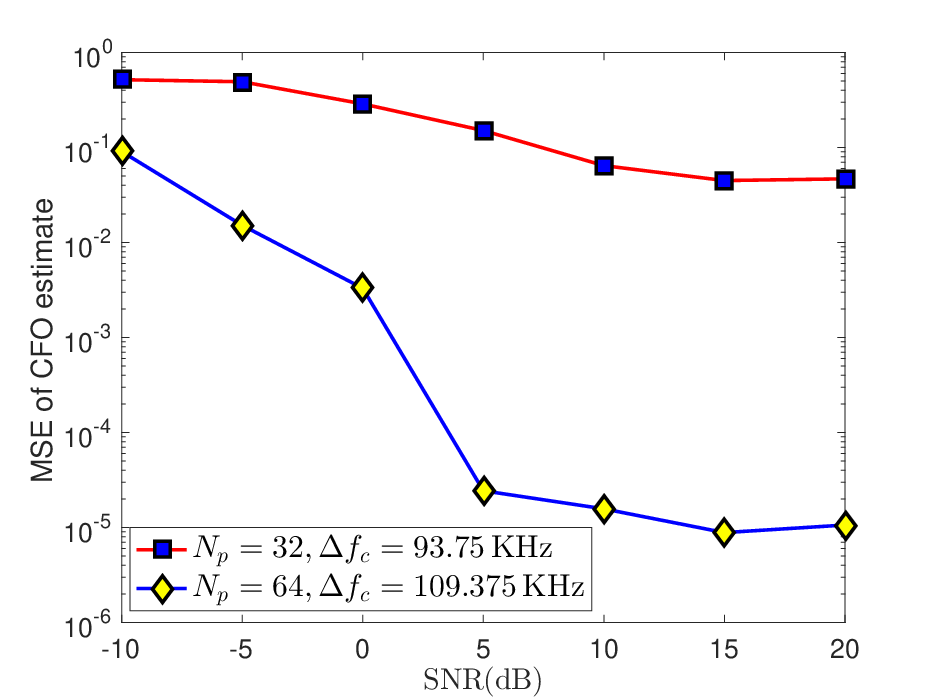
The CFO in typical wireless systems is of the order of parts per millions (ppms) of the carrier frequency. For each of the training lengths, the CFO ($\Delta f_{c}$) is chosen to be within the practical limits and maximally off grid for a DFT bin width of ${1}/{N_{\mathrm{p}}T}$. Therefore, we choose $\omega_{e}=2\pi\Delta f_{c}T$ corresponding to $\Delta f_{c}=93.75\,\mathrm{KHz}$ and $109.375\,\mathrm{KHz}$ for $N_{\mathrm{p}}=32$ and $64$ respectively. We evaluate our joint estimation algorithm using the Normalised Mean Square Error (NMSE) of the channel estimate ($\hat{\mathbf{H}}$), the lower bound on the achievable rate ($\mathbf{R}$) and the mean square error (MSE) of the CFO estimate $\left(\hat{\omega}_{e}\right)$. The NMSE of the channel estimate is defined as the average of ${\left\|\mathbf{H}-\gamma\hat{\mathbf{H}}\right\|_{F}}/{\left\|\mathbf{H}\right\|_{F}}$ for several realizations of $\mathbf{H}$, where $\gamma=\underset{a}{\mathrm{arg\,min}}\left\|\mathbf{H}-a\hat{\mathbf{H}}\right\|_{F}$ for a given $\mathbf{H}$, $\hat{\mathbf{H}}$. Neglecting the training overhead due to channel estimation, we evaluate the lower bound on the achievable rate using the expression in [12], which is derived using a linearization approximation of the quantization function $\mathcal{Q}_{1}\left(.\right)$. The MSE of the CFO estimate is given by $\mathbb{E}\left[\left(\omega_{e}-\hat{\omega}_{e}\right)^{2}\right]$, where the expectation is found by the empirical average over several realizations of the channel matrix and the training. Simulation results suggest that with few pilots, our algorithm performs the joint estimation within acceptable limits, even with the heavily constrained hardware.

We have proposed a joint CFO and channel estimation technique for narrowband mmWave systems using low resolution ADCs at the receivers. The key idea of our paper is to jointly model the CFO-channel problem using lifting techniques, solve a noisy quantized compressed sensing problem using the EM-GAMP and recover the components corresponding to CFO and channel using the SVD. Our method exploits the sparsity of the mmWave channel matrix in the angle domain and is able to perform joint estimation compressively. In our future work, we will consider frame synchronization in addition to CFO and channel estimation, address the computational complexity issues associated with lifting, and extend our work to wideband systems using low resolution ADCs.

References

- [1] R. W. Heath, N. Gonzalez-Prelcic, S. Rangan, W. Roh, and A. M. Sayeed, “An overview of signal processing techniques for millimeter wave MIMO systems,” IEEE J. Sel. Topics Signal Process., vol. 10, no. 3, pp. 436–453, 2016.
- [2] A. Alkhateeb, G. Leus, and R. W. Heath, “Compressed sensing based multi-user millimeter wave systems: How many measurements are needed?” in Proc. of the IEEE Int. Conf. Acoust., Speech Signal Process.(ICASSP), 2015, pp. 2909–2913.
- [3] D. Ramasamy, S. Venkateswaran, and U. Madhow, “Compressive parameter estimation in AWGN,” IEEE Trans. Signal Process., vol. 62, no. 8, pp. 2012–2027, Aug. 2014.
- [4] J. Mo, P. Schniter, N. G. Prelcic, and R. W. Heath, “Channel estimation in millimeter wave MIMO systems with one-bit quantization,” in Proc. of the Asilomar Conference on Signals, Systems and Computers, 2014, pp. 957–961.
- [5] O. Abari, H. Hassanieh, M. Rodreguez, and D. Katabi, “Millimeter wave communications: From point-to-point links to agile network connections,” in Proc. of the ACM Workshop on Hot Topics in Networks, 2016, pp. 169–175.
- [6] Z. Lin, X. Peng, and F. Chin, “Joint carrier frequency offset and channel estimation for OFDM based gigabit wireless communication system with low precision ADC,” in Proc. of the IEEE Vehicular Technology Conference (VTC Fall), 2011, pp. 1–5.
- [7] Y. Fu, C. Tellambura, and W. A. Krzymien, “Limited-feedback precoding for closed-loop multiuser MIMO OFDM systems with frequency offsets,” IEEE Transactions on Wireless Communications, vol. 7, no. 11, 2008.
- [8] S. Ling and T. Strohmer, “Self-calibration and biconvex compressive sensing,” Inverse Problems, vol. 31, no. 11, p. 115002, 2015.
- [9] J. P. Vila and P. Schniter, “Expectation-maximization gaussian-mixture approximate message passing,” IEEE Transactions on Signal Processing, vol. 61, no. 19, pp. 4658–4672, 2013.
- [10] E. J. Candes, T. Strohmer, and V. Voroninski, “Phaselift: Exact and stable signal recovery from magnitude measurements via convex programming,” Commun. on Pure and Applied Mathematics, vol. 66, no. 8, pp. 1241–1274, 2013.
- [11] S. Rangan, “Generalized approximate message passing for estimation with random linear mixing,” in IEEE International Symposium on Information Theory, 2011, pp. 2168–2172.
- [12] J. Mo, P. Schniter, and R. W. Heath Jr, “Channel estimation in broadband millimeter wave MIMO systems with few-bit ADCs,” arXiv preprint arXiv:1610.02735v2, 2017.
- [13] C. Candan, “A method for fine resolution frequency estimation from three DFT samples.” IEEE Signal Process. Lett., vol. 18, no. 6, pp. 351–354, 2011.