Centrality measures for graphons: Accounting for uncertainty in networks
Abstract
As relational datasets modeled as graphs keep increasing in size and their data-acquisition is permeated by uncertainty, graph-based analysis techniques can become computationally and conceptually challenging. In particular, node centrality measures rely on the assumption that the graph is perfectly known — a premise not necessarily fulfilled for large, uncertain networks. Accordingly, centrality measures may fail to faithfully extract the importance of nodes in the presence of uncertainty. To mitigate these problems, we suggest a statistical approach based on graphon theory: we introduce formal definitions of centrality measures for graphons and establish their connections to classical graph centrality measures. A key advantage of this approach is that centrality measures defined at the modeling level of graphons are inherently robust to stochastic variations of specific graph realizations. Using the theory of linear integral operators, we define degree, eigenvector, Katz and PageRank centrality functions for graphons and establish concentration inequalities demonstrating that graphon centrality functions arise naturally as limits of their counterparts defined on sequences of graphs of increasing size. The same concentration inequalities also provide high-probability bounds between the graphon centrality functions and the centrality measures on any sampled graph, thereby establishing a measure of uncertainty of the measured centrality score.
Index Terms:
Random graph theory, Networks, Graphons, Centrality measures, Stochastic block modelI Introduction
Many biological [1], social [2], and economic [3] systems can be better understood when interpreted as networks, comprising a large number of individual components that interact with each other to generate a global behavior. These networks can be aptly formalized by graphs, in which nodes denote individual entities, and edges represent pairwise interactions between those nodes. Consequently, a surge of studies concerning the modeling, analysis, and design of networks have appeared in the literature, using graphs as modeling devices.
A fundamental task in network analysis is to identify salient features in the underlying system, such as key nodes or agents in the network. To identify such important agents, researchers have developed centrality measures in various contexts [4, 5, 6, 7, 8], each of them capturing different aspects of node importance. Prominent examples for the utility of centrality measures include the celebrated PageRank algorithm [9, 10], employed in the search of relevant sites on the web, as well as the identification of influential agents in social networks to facilitate viral marketing campaigns [11].
A crucial assumption for the applicability of these centrality measures is that the observation of the underlying network is complete and noise free. However, for many systems we might be unable to extract a complete and accurate graph-based representation, e.g., due to computational or measurement constraints, errors in the observed data, or because the network itself might be changing over time. For such reasons, some recent approaches have considered the issue of robustness of centrality measures [12, 13, 14, 15] and general network features [16], as well as their computation in dynamic graphs [17, 18, 19]. The closest work to ours is [20], where convergence results are derived for eigenvector and Katz centralities in the context of random graphs generated from a stochastic block model.
As the size of the analyzed systems continues to grow, traditional tools for network analysis have been pushed to their limit. For example, systems such as the world wide web, the brain, or social networks can consist of billions of interconnected agents, leading to computational challenges and the irremediable emergence of uncertainty in the observations. In this context, graphons have been suggested as an alternative framework to analyze large networks [21, 22]. While graphons have been initially studied as limiting objects of large graphs [23, 24, 25], they also provide a rich non-parametric modeling tool for networks of any size [26, 27, 28, 29]. In particular, graphons encapsulate a broad class of network models including the stochastic block model [30, 31], random dot-product graphs [32], the infinite relational model [33], and others [34]. A testament of the practicality of graphons is their use in applied disciplines such as signal processing [35], collaborative learning [36], and control [37].
In this work we aim at harnessing the additional flexibility provided by the graphon framework to suggest a statistical approach to agents’ centralities that inherently accounts for network uncertainty, as detailed next.
I-A Motivation
Most existing applications of network centrality measures follow the paradigm in Fig. 1a: a specific graph — such as a social network with friendship connections — is observed, and conclusions about the importance of each agent are then drawn based on this graph, e.g., which individuals have more friends or which have the most influential connections. Mathematically, these notions of importance are encapsulated in a centrality measure that ranks the nodes according to the observed network structure. For instance, the idea that importance derives from having the most friends is captured by degree centrality. Since the centrality of any node is computed solely from the network structure [4, 5, 6, 7, 8], a crucial assumption hidden in this analysis is that the empirically observed network captures all the data we care about.
However, in many instances in which centrality measures are employed, this assumption is arguably not fulfilled: we typically do not observe the complete network at once. Further, even those parts we observe contain measurement errors, such as false positive or false negative links, and other forms of uncertainty. The key question is therefore how to identify crucial nodes via network-based centrality measures without having access to an accurate depiction of the ‘true’ latent network.
One answer to this problem is to adopt a statistical inference-based viewpoint towards centrality measures, by assuming that the observed graph is a specific realization of an underlying stochastic generative process; see Fig. 1b. In this work, in particular, we use graphons to model such underlying generative process, because they provide a rich non-parametric statistical framework. Further, it has been recently shown that graphons can be efficiently estimated from one (or multiple) noisy graph observations [28, 38]. Our main contribution is to show that, based on the inferred graphon, one can compute a latent centrality profile of the nodes that we term graphon centrality function. This graphon centrality may be seen as a fundamental measure of node importance, irrespective of the specific realization of the graph at hand. This leads to a robust estimate of the centrality profiles of all nodes in the network. In fact, we provide high-probability bounds between the distance of such latent graphon centrality functions and the centrality profiles in any realized network, in terms of the network size.

To illustrate the dichotomy of the standard approach towards centrality and the one outlined here, let us consider the graphon in Fig. 1c. Graphons will be formally defined in Section II-B, but the fundamental feature is that it defines a random graph model from where graphs of any pre-specified size can be obtained. If we generate one of these graphs with nodes, we can apply the procedure in Fig. 1a to obtain a centrality value for each agent, as shown in the red curve in Fig. 1c. In the standard paradigm we would then sort the centrality values to find the most central nodes, which in this case would correspond to the node marked as in Fig. 1c. On the other hand, if we have access to the generative graphon model (or an estimate thereof), then we can compute the continuous graphon centrality function and compare the deviations from it in the specific graph realization; see blue and red curves in Fig. 1c.
The result is that while is the most central node in the specific graph realization (see red curve), we would expect it to be less central within the model-based framework since the two nodes to its right have higher latent centrality (see blue curve). Stated differently, in this specific realization, benefited from the random effects in terms of its centrality. If another random graph is drawn from the same graphon model, the rank of might change, e.g., node might become less central. Based on a centrality analysis akin to Fig. 1a, we would conclude that the centrality of this node decreased relative to other agents in the network. However, this difference is exclusively due to random variations and thus not statistically significant. The approach outlined in Fig. 1b and, in particular, centrality measures defined on graphons thus provide a statistical framework to analyze centralities in the presence of uncertainty, shielding us from making the wrong conclusion about the change in centrality of node if the network is subject to uncertainty.
A prerequisite to apply the perspective outlined above is to have a consistent theory of centrality measures for graphons, with well-defined limiting behaviors and well-understood convergence rates. Such a theory is developed in this paper, as we detail in the next section.
I-B Contributions and article structure
Our contributions are listed below.
1) We develop a theoretical framework and definitions for centrality measures on graphons.
Specifically, using the existing spectral theory of linear integral operators, we define the degree, eigenvector, Katz and PageRank centrality functions (see Definition 3).
2) We discuss and illustrate three different analytical approaches to compute such centrality functions (see Section IV).
3) We derive concentration inequalities showing that our newly defined graphon centrality functions are natural limiting objects of centrality measures for finite graphs. These concentration inequalities improve the current state of the art and constitute the main technical results of this paper (see Theorems V and V).
4) We illustrate how such bounds can be used to quantify the distance between the latent graphon centrality function and the centrality measures of finite graphs sampled from the graphon.
The remainder of the article is structured as follows. In Section II we review preliminaries regarding graphs, graph centralities, and graphons. Subsequently, in Section III we recall the definition of the graphon operator and use it to introduce centrality measures for graphons. Section IV discusses how centrality measures for graphons can be computed using different strategies, and provides some detailed numerical examples. Thereafter, in Section V, we derive our main convergence results. Section VI provides concluding remarks. Appendix A contains proofs omitted in the paper. Appendix B provided in the supplementary material presents some auxiliary results and discussions.
Notation: The entries of a matrix and a (column) vector are denoted by and , respectively; however, in some cases and are used for clarity. The notation T stands for transpose. is a diagonal matrix whose th diagonal entry is . denotes the ceiling function that returns the smallest integer larger than or equal to . Sets are represented by calligraphic capital letters, and denotes the indicator function over the set . , , , and refer to the all-zero vector, the all-one vector, the -th canonical basis vector, and the identity matrix, respectively. The symbols , , and are reserved for eigenvectors, eigenfunctions, and eigenvalues, respectively. Additional notation is provided at the beginning of Section III.
II Preliminaries
In Section II-A we introduce basic graph-theoretic concepts as well as the notion of node centrality measures for finite graphs, emphasizing the four measures studied throughout the paper. A brief introduction to graphons and their relation to random graph models is given in Section II-B.
II-A Graphs and centrality measures
An undirected and unweighted graph consists of a set of nodes or vertices and an edge set of unordered pairs of elements in . An alternative representation of such a graph is through its adjacency matrix , where if and otherwise. In this paper we consider simple graphs (i.e., without self-loops), so that for all .
Node centrality is a measure of the importance of a node within a graph. This importance is not based on the intrinsic nature of each node, but rather on the location that the nodes occupy within the graph. More formally, a centrality measure assigns a nonnegative centrality value to every node such that the higher the value, the more central the node is. The centrality ranking imposed on the node set is in general more relevant than the absolute centrality values. Here, we focus on four centrality measures, namely, the degree, eigenvector, Katz and PageRank centrality measures overviewed next; see [8] for further details.
Degree centrality is a local measure of the importance of a node within a graph. The degree centrality of a node is given by the number of nodes connected to , that is,
| (1) |
where the vector collects the values of for all .
Eigenvector centrality, just as degree centrality, depends on the neighborhood of each node. However, the centrality measure of a given node does not depend only on the number of neighbors, but also on how important those neighbors are. This recursive definition leads to an equation of the form , i.e., the vector of centralities is an eigenvector of . Since is symmetric, its eigenvalues are real and can be ordered as . The eigenvector centrality is then defined as the principal eigenvector , associated with :
| (2) |
For connected graphs, the Perron-Frobenius theorem guarantees that is a simple eigenvalue, and that there is a unique associated (normalized) eigenvector with positive real entries. As will become apparent later, the normalization introduced in (2) facilitates the comparison of the eigenvector centrality on a graph to the corresponding centrality measure defined on a graphon.
Katz centrality measures the importance of a node based on the number of immediate neighbors in the graph as well as the number of two-hop neighbors, three-hop neighbors, and so on. The effect of nodes further away is discounted at each step by a factor . Accordingly, the vector of centralities is computed as , where we add the number of k-hop neighbors weighted by . By choosing such that , the above series converges and we can write the Katz centrality compactly as
| (3) |
Notice that if is close to zero, the relative weight given to neighbors further away decreases fast, and is driven mainly by the one-hop neighbors just like degree centrality. In contrast, if is close to , the solution to (3) is almost a scaled version of . Intuitively, for intermediate values of , Katz centrality captures a hybrid notion of importance by combining elements from degree and eigenvector centralities. We remark that Katz centrality is sometimes defined as . Since a constant shift does not alter the centrality ranking, we here use formula (3). We also note that Katz centrality is sometimes referred to as Bonacich centrality in the literature.
PageRank measures the importance of a node in a recursive way based on the importance of the neighboring nodes (weighted by their degree). Mathematically, the PageRank centrality of node is given by
| (4) |
where and is the diagonal matrix of the degrees of the nodes. Note that the above formula corresponds to the stationary distribution of a random ‘surfer’ on a graph, who follows the links on the graph with probability and with probability jumps (‘teleports’) to a uniformly at random selected node in the graph. See [10] for further details on PageRank.
II-B Graphons
A graphon is the limit of a convergent sequence of graphs of increasing size, that preserves certain desirable features of the graphs contained in the sequence [23, 24, 25, 22, 21, 39, 40, 41]. Formally, a graphon is a measurable function that is symmetric . Intuitively, one can interpret the value as the probability of existence of an edge between and . However, the ‘nodes’ and no longer take values in a finite node set as in classical finite graphs but rather in the continuous interval . Based on this intuition, graphons also provide a natural way of generating random graphs [42, 39], as introduced in the seminal paper [23] under the name -random graphs. In this paper we will make use of the following model, in which the symmetric adjacency matrix of a simple random graph of size constructed from a graphon is such that for all
| (5) |
where and are latent variables selected uniformly at random from , and is a constant regulating the sparsity of the graph (see also Definition 7)11 1 Throughout this paper we adopt the terminology of sparse graphs for graphs generated following (5) with parameter and as , even though this does not imply a bounded degree. This terminology is consistent with common usage in the literature [43, 44, 45]. Note also that [46] proposed an interesting graph limit framework for graph sequences with bounded degree.
This means that, when conditioned on the latent variables , the off-diagonal entries of the symmetric matrix are independent Bernoulli random variables with success probability given by . In this sense, when , the constant graphon gives rise to Erdős-Rényi random graphs with edge probability . Analogously, a piece-wise constant graphon gives rise to stochastic block models [30, 31]; for more details see Section IV-A. Interestingly, it can be shown that the distribution of any simple exchangeable random graph [39, 34] is characterized by a function as discussed above [47, 48, 39]. Finally, observe that for any measure preserving map , the graphons and define the same probability distribution on random graphs. A precise characterization of the equivalence classes of graphons defining the same probability distribution can be found in [22, Ch. 10].
III Extending centralities to graphons
In order to introduce centrality measures for graphons we first introduce a linear integral operator associated with a graphon and recall its spectral properties. From here on, we denote by the Hilbert function space with inner product for , and norm . The elements of are the equivalence classes of Lebesgue integrable functions , that is, we identify two functions and with each other if they differ only on a set of measure zero (i.e., ). is the identity function in . We use blackboard bold symbols (such as ) to denote linear operators acting on , with the exception of and that denote the sets of natural and real numbers. The induced (operator) norm is defined as .
III-A The graphon integral operator and its properties
Following [22], we introduce a linear operator that is fundamental to derive the notions of centrality for graphons.
Definition 1 (Graphon operator).
For a given graphon , we define the associated graphon operator as the linear integral operator
From an operator theory perspective, the graphon is the integral kernel of the linear operator . Given the key importance of , we review its spectral properties in the next definition and lemma.
Definition 2 (Eigenvalues and eigenfunctions).
A complex number is an eigenvalue of if there exists a nonzero function , called the eigenfunction, such that
| (6) |
It follows from the above definition that the eigenfunctions are only defined up to a rescaling parameter. Hence, from now on we assume all eigenfunctions are normalized such that
We next recall some known properties of the graphon operator.
Lemma 1.
The graphon operator has the following properties.
1) is self-adjoint, bounded, and continuous.
2) is diagonalizable.
Specifically, has countably many eigenvalues, all of which are real and can be ordered as .
Moreover, there exists an orthonormal basis for of eigenfunctions .
That is, for all and any function can be decomposed as
Consequently,
If the set of nonzero eigenvalues is infinite, then is its unique accumulation point.
3) Let denote consecutive applications of the operator .
Then, for any ,
4) The maximum eigenvalue is positive and there exists an associated eigenfunction which is positive, that is, for all . Moreover, .
III-B Definitions of centrality measures for graphons
We define centrality measures for graphons based on the graphon operator introduced in the previous section. These definitions closely parallel the construction of centrality measures in finite graphs; see Section II-A. The main difference is that the linear operator defining the respective centralities is an infinite dimensional operator, rather than a finite dimensional matrix.
Definition 3 (Centrality measures for graphons).
Given a graphon and its associated operator , we define the following centrality functions:
-
1) Degree centrality: We define as
(7) -
2) Eigenvector centrality: For with a simple largest eigenvalue , let () be the associated positive eigenfunction. The eigenvector centrality function is
(8) -
3) Katz centrality: Consider the operator where . For any , we define the Katz centrality function as
(9) -
4) PageRank centrality: Consider the operator
where if and if . For any , we define as
(10) Note that implies almost everywhere.
Remark 1.
The Katz centrality function is well defined, since for the operator is invertible [50, Theorem 2.2]. Moreover, denoting the identity operator by , it follows that . Hence, by using a Neumann series representation and the properties of the higher order powers of we obtain the equivalent representation
where we used that for all . Using an analogous series representation it can be shown that PageRank is well defined. Note also that eigenvector centrality is well-defined by Lemma 1, part 4).
Since a graphon describes the limit of an infinite dimensional graph, there is a subtle difference in the semantics of the centrality measure compared to the finite graph setting. Specifically, in the classical setting the network consists of a finite number of nodes and thus for a graph of nodes we obtain an -dimensional vector with one centrality value per node. In the graphon setting, we may think of each real as corresponding to one of infinitely many nodes, and thus the centrality measure is described by a function.
IV Computing centralities on graphons
We illustrate how to compute centrality measures for graphons by studying three examples in detail. The graphons we consider are ordered by increasing complexity of their respective eigenspaces and by the generality of the methods used in the computation of the centralities.
IV-A Stochastic block model graphons
We consider a class of piecewise constant graphons that may be seen as the equivalent of a stochastic block model (SBM). Such graphons play an important role in practice, as they enable us to approximate more complicated graphons in a ‘stepwise’ fashion. This approximation idea has been exploited to estimate graphons from finite data [28, 51, 52]. In fact, optimal statistical rates of convergence can be achieved over smooth graphon classes [53, 45]. The SBM graphon is defined as follows
| (11) |
where , , and for . We define the following dimensional vector of indicator functions
| (12) |
enabling us to compactly rewrite the graphon in (11) as
| (13) |
We also define the following auxiliary matrices.
Definition 4.
Let us define the effective measure matrix and the effective connectivity matrix for SBM graphons as follows
| (14) |
Notice that is a diagonal matrix with entries collecting the sizes of each block. Similarly, the matrix is obtained by weighting the probabilities in by the sizes of the different blocks. Hence, the effective connectivity from block to two blocks and may be equal even if the latter block has twice the size (), provided that it has half the probability of edge appearance (). Notice also that the matrix need not be symmetric. As will be seen in Section IV-B, the definitions in (14) are specific examples of more general constructions.
The following lemma relates the spectral properties of to those of the operator induced by . We do not prove this lemma since it is a special case of Lemma 3, introduced in Section IV-B and shown in Appendix A.
Lemma 2.
Let and denote the eigenvalues and eigenvectors of in (14), respectively. Then, all the nonzero eigenvalues of are given by and the associated eigenfunctions are of the form .
Using the result above, we can compute the centrality measures for stochastic block model graphons based on the effective connectivity matrix.
Proposition 1 (Centrality measures for SBM graphons).
Let and denote the eigenvalues and eigenvectors of in (14), respectively, and define the diagonal matrix . The centrality functions , , , and of the graphon can be computed as follows
| (15) | ||||
We next illustrate this result with an example. Its proof is given in Appendix A.
IV-A1 Example of a stochastic block model graphon
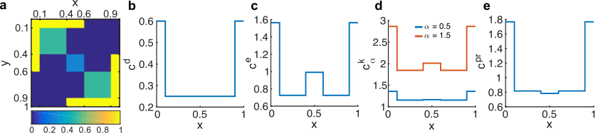
Consider the stochastic block model graphon depicted in Fig. 2-(a), with corresponding symmetric matrix [cf. (11)] as in (16). Let us define the vector of indicator functions specific to this graphon , where the blocks coincide with those in Fig. 2-(a), that is, , , , , and . To apply Proposition 1 we need to compute the effective measure and effective connectivity matrices [cf. (14)], which for our example are given by
| (16a) | |||
| (16b) | |||
The principal eigenvector of is given by . Furthermore, from (15) we can compute the graphon centrality functions to obtain
where for illustration purposes we have evaluated the Katz centrality for two specific choices of , and we have set for the PageRank centrality. These four centrality functions are depicted in Fig. 2(b)-(e).
Note that these functions are piecewise constant according to the block partition . Moreover, as expected from the functional form of in Fig. 2-(a), blocks and are the most central as measured by any of the four studied centralities. Regarding the remaining three blocks, degree centrality deems them as equally important whereas eigenvector centrality considers to be more important than and . To understand this discrepancy, notice that in any finite realization of the graphon , most of the edges from a node in block will go to nodes in and , which are the most central ones. On the other hand, for nodes in blocks and , most of the edges will be contained within their own block. Hence, even though nodes corresponding to blocks , , and have the same expected number of neighbors – thus, same degree centrality – the neighbors of nodes in tend to be more central, entailing a higher eigenvector centrality. As expected, an intermediate situation occurs with Katz centrality, whose form is closer to degree centrality for lower values of (cf. ) and closer to eigenvector centrality for larger values of this parameter (cf. ). For the case of PageRank, on the other hand, block is deemed as less central than and . This can be attributed to the larger size of these latter blocks. Indeed, the classical PageRank centrality measure is partially driven by size [10].
IV-B Finite-rank graphons
We now consider a class of finite-rank (FR) graphons that can be written as a finite sum of products of integrable functions. Specifically, we consider graphons of the form
| (17) |
where and we have defined the vectors of functions and . Observe that and must be chosen so that is symmetric, and for all . Based on and we can define the generalizations of and introduced in Section IV-A, for this class of finite-rank graphons.
Definition 5.
The effective measure matrix and the effective connectivity matrix for a finite-rank graphon as defined in (17) are given by
| (18) |
The stochastic block model graphon operator introduced in (11) is a special case of the class of operators in (17). More precisely, we recover the SBM graphon by choosing and for . The matrices defined in (14) are recovered when specializing Definition 5 to this choice of and . We may now relate the eigenfunctions of the FR graphon with the spectral properties of , as explained in the following lemma.
Lemma 3.
Lemma 3 is proven in Appendix A and shows that the graphon in (17) is of finite rank since it has at most non-zero eigenvalues. Notice that Lemma 2 follows from Lemma 3 when specializing the finite rank operator to the SBM case as explained after Definition 5. Moreover, we can leverage the result in Lemma 3 to find closed-form expressions for the centrality functions of FR graphons. To write these expressions compactly, we define the vectors of integrated functions and , as well as the following normalized versions of and
| (19) |
With this notation in place, we can establish the following result, which is proven in Appendix A.
Proposition 2 (Centrality measures for FR graphons).
Let be the principal eigenvector of in (18). Then, the centrality functions , , , and of the graphon can be computed as follows
| (20) | ||||
In the next subsection we illustrate the use of Proposition 2 for the computation of graphon centralities.
IV-B1 Example of a finite-rank graphon
Consider the FR graphon given by
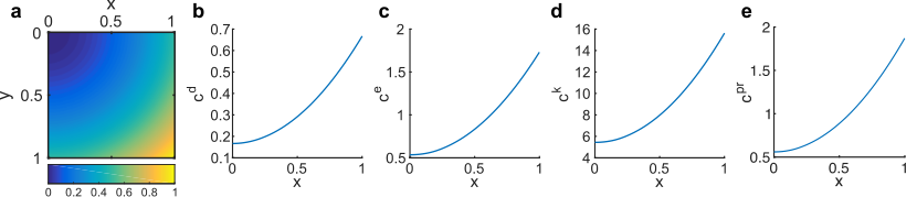
and illustrated in Fig. 3-(a). Notice that this FR graphon can be written in the canonical form (17) by defining the vectors and . From (18) we then compute the relevant matrices and , as well as the relevant normalized quantities, to obtain
A simple computation reveals that the principal eigenvector of is . We now leverage the result in Proposition 2 to obtain
where we have set in the PageRank centrality. Moreover, we have evaluated the Katz centrality for , where is the largest eigenvalue of . The four centrality functions are depicted in Fig. 3-(b) through (e). As anticipated from the form of , there is a simple monotonicity in the centrality ranking for all the measures considered. More precisely, highest centrality values are located close to in the interval , whereas low centralities are localized close to . Unlike in the example of the stochastic block model in Section IV-A1, all centralities here have the same functional form of a quadratic term with a constant offset.
IV-C General smooth graphons
In general, a graphon need not induce a finite-rank operator as in the preceding Sections IV-A and IV-B. However, as shown in Lemma 1, a graphon always induces a diagonalizable operator with countably many nonzero eigenvalues. In most cases, obtaining the degree centrality function is immediate since it entails the computation of an integral [cf. (7)]. On the other hand, for eigenvector, Katz, and PageRank centralities that depend on the spectral decomposition of , there is no universal technique available. Nonetheless, a procedure that has shown to be useful in practice to obtain the eigenfunctions and corresponding eigenvalues of smooth graphons is to solve a set of differential equations obtained by successive differentiation, when possible, of the eigenfunction equation in (6), that is, by considering
| (21) |
for . In the following section we illustrate this technique on a specific smooth graphon that does not belong to the finite-rank class.
IV-C1 Example of a general smooth graphon
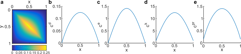
Consider the graphon depicted in Fig. 4-(a) and with the following functional form
Specializing the differential equations in (21) for graphon we obtain
| (22) |
First notice that without differentiating (i.e. for ) we can determine the boundary conditions . Moreover, by computing the second derivatives in (22), we obtain that . From the solution of this differential equation subject to the boundary conditions it follows that the eigenvalues and eigenfunctions of the operator are
| (23) |
Notice that has an infinite — but countable — number of nonzero eigenvalues, with an accumulation point at zero. Thus, cannot be written in the canonical form for finite-rank graphons (17). Nevertheless, having obtained the eigenfunctions we can still compute the centrality measures for . For degree centrality, a simple integration gives us
From (23) it follows that the principal eigenfunction is achieved when . Thus, the eigenvector centrality function [cf. (8)] is given by
Finally, for the Katz centrality we leverage Remark 1 and the eigenfunction expressions in (23) to obtain
which is guaranteed to converge as long as . We plot these three centrality functions in Fig. 4-(b) through (d), where we selected for the Katz centrality. Also, in Fig. 4-(e) we plot an approximation to the PageRank centrality function obtained by solving numerically the integral in its definition. According to all centralities, the most important nodes within this graphon are those located in the center of the interval , in line with our intuition. Likewise, nodes at the boundary have low centrality values. Note that while the ranking according to all centrality functions is consistent, unlike in the example in Section IV-B1, here there are some subtle differences in the functional forms. In particular, degree centrality is again a quadratic function whereas the eigenvector and Katz centralities are of sinusoidal form.
V Convergence of centrality measures
In this section we derive concentration inequalities relating the newly defined graphon centrality functions with standard centrality measures. To this end, we start by noting that while graphon centralities are functions, standard centrality measures are vectors. To be able to compare such objects, we first show that there is a one to one relation between any finite graph with adjacency matrix and a suitably constructed stochastic block model graphon . Consequently, any centrality measure of is in one to one relation with the corresponding centrality function of . To this end, for each , we define a partition of into the intervals , where for , and . We denote the associated indicator-function vector by consistently with (12).
Lemma 4.
For any adjacency matrix define the corresponding stochastic block model graphon as
Then the centrality function corresponding to the graphon is given by
where is the centrality measures of the graph with rescaled adjacency matrix .
Proof.
Remark 2.
Note that the scaling factor does not affect the centrality rankings of the nodes in , but only the magnitude of the centrality measures. This re-scaling is needed to avoid diverging centrality measures for graphs of increasing size. Observe further that is the piecewise-constant function corresponding to the vector . We finally remark that graphons of the type have appeared before in the literature using a different notation [24].
By using the previous lemma, we can compare centralities of graphons and graphs by working in the function space. Using this equivalence, we demonstrate that the previously defined graphon centrality functions are not only defined analogously to the centrality measures on finite graphs, but also emerge as the limit of those centrality measures for a sequence of graphs of increasing size. Stated differently, just like the graphon provides an appropriate limiting object for a growing sequence of finite graphs, the graphon centrality functions can be seen as the appropriate limiting objects of the finite centrality measures as the size of the graphs tends to infinity. In this sense, the centralities presented here may be seen as a proper generalization of the finite setting, just like a graphon provides a generalized framework for finite graphs. Most importantly, we show that the distance (in norm) between the graphon centrality function and the step-wise constant function associated with the centrality vector of any graph sampled from the graphon can be bounded, with high probability, in terms of the sampled graph size .
Definition 6 (Sampled graphon).
Given a graphon and a size fix the latent variables by choosing either:
- -
‘deterministic latent variables’: .
- -
‘stochastic latent variables’: where is the -th order statistic of random samples from .
Utilizing such latent variables construct
- -
the ‘probability’ matrix
- -
the sampled graphon
- -
the operator of the sampled graphon
The sampled graphon obtained when working with deterministic latent variables can intuitively be seen as an approximation of the graphon by using a stochastic block model graphon with blocks, as the one described in Section IV-A, and is useful to study graphon centrality functions as limit of graph centrality measures. On the other hand, the sampled graphon obtained when working with stochastic latent variables is useful as an intermediate step to analyze the relation between the graphon centrality function and the centrality measure of graphs sampled from the graphon according to the following procedure.
Definition 7 (Sampled graph).
Given the ‘probability’ matrix of a sampled graphon we define
- -
the sampled matrix as the adjacency matrix of a symmetric (random) graph obtained by taking isolated vertices , and adding undirected edges between vertices and at random with probability for all . Note that .
- -
the associated (random) linear operator
(24) and its associated (random) graphon:
(25)
In general, we denote the centrality functions associated with the sampled graphon operator by whereas the centrality functions associated with the operator are denoted by . Note that thanks to Lemma 4 such centrality functions are in one to one correspondence with the centrality measures of the finite graphs and , respectively. Consequently, studying the relation between , and allows us to relate the graphon centrality function with the centrality measure of graphs sampled from the graphon. We note that previous works on graph limit theory imply the convergence of and to the graphon operator [25, 54, 22]. Intuitively, convergence of and to then follows from continuity of spectral properties of the graphon operator. In the following, we make this argument precise and more importantly we provide a more refined analysis by establishing sharp rates of convergence of the sampled graphs, under the following smoothness assumption on . A more detailed discussion of related convergence results can be found in Appendix B (see supplementary material).
Assumption 1 (Piecewise Lipschitz graphon).
There exists a constant and a sequence of non-overlapping intervals defined by , for a (finite) , such that for any , any set and pairs , we have that
This assumption has also been used in the context of graphon estimation [28, 53] and is typically fulfilled for most of the graphons of interest.
[Convergence of graphon operators] For a graphon fulfilling Assumption 1, it holds with probability that:
| (26) | ||||
where and in the case of deterministic latent variables and and in the case of stochastic latent variables. Moreover, if is large enough, as specified in Lemma 5, then with probability at least
| (27) |
In particular, if with , then:
| (28) |
Remark 3.
To control the error induced by the random sampling, we derive a concentration inequality for uniform order statistics, as reported next, that can be of independent interest. As this result is not central to the discussion of our paper, we relegate its proof to Appendix B. In addition, we make use of a lower bound on the maximum expected degree as reported in Lemma 5 and proven in Appendix B.
Proposition 3.
Let be the order statistics of points sampled from a standard uniform distribution. Suppose that and . With probability at least
Lemma 5.
If is such that
| (29a) | |||
| (29b) |
then .
Proof of Theorem V:
We prove the three statements sequentially.
Proof of (26).
First of all note that by definition, for any it holds
but it is not necessarily true that .
Let us define such that the point belongs to the Lipschitz block , as defined in Assumption 1 and illustrated in Fig. 5.
We define as the subset of points in that belong to the same Lipschitz block as . Mathematically,

In the following, we partition the set into the set and its complement . In words, is the set of points, for which and its corresponding sample belong to the same Lipschitz block. We now prove that, with probability , has area
| (30) |
To prove the above, we define the set by constructing a stripe of width centered at each discontinuity of the graphon, as specified in Assumption 1. This guarantees that any point in has distance more than component-wise from a discontinuity.
Note that in the case of deterministic latent variables for any and any it holds by construction that and similarly . In the case of stochastic latent variables, Proposition 3 guarantees that with probability at least for any and any it holds , . In both cases, with probability , all the points in are less than close to their sample and more than far from any discontinuity (component-wise) hence they surely belong to .
Consequently, with probability we have . Each stripe in has width , length , and there are stripes in total. Formula (30) is then immediate by noticing that multiplying times counts twice the intersections between horizontal and vertical stripes.
Consider now any such that . Let and note that . Then we get
| (31) | ||||
| (32) |
Expression (31) follows from the Cauchy-Schwarz inequality; we used and, in the last equation, we split the interval into the sets and , as described above and illustrated in Fig. 5.
We can now bound both terms in (32). For the first term, note that for all the points in the corresponding sample belongs to the same Lipschitz block and is at most apart (component-wise). Consequently, for these points Overall, we get
For the second term in (32), we use (30) and the fact that to get
Substituting these two terms into (32) yields
Since this bound holds for all functions with unit norm, we recover (26).
Proof of (27). From the triangle inequality we get that
| (33) |
We have already bounded the second term on the right hand side of (33), so we now concentrate on the first term.
The operator can be seen as the graphon operator of an SBM graphon with matrix . By Lemma 2 we then have that its eigenvalues coincide with the eigenvalues of the corresponding matrix which is since in this case (given that all the intervals have length ).22 2 Note that Lemma 2 is formulated for graphon operators (i.e. linear integral operators with nonnegative kernels). An identical proof shows that the result holds also if the kernel assumes negative values. Consequently,
Hence, to bound the norm of the difference between a random SBM graphon operator based on the graphon , with , and its expectation defined via the graphon , we can employ matrix concentration inequalities. Specifically, we use [55, Theorem 1] in order to bound the deviations of .
By Lemma 5, for large enough, the maximum expected degree of the random graph represented by grows at least as . Consequently, all the conditions of [55, Theorem 1] are met and we get that with probability
where we used that since each element in belongs to .
Proof of (28). We finally show that (27) implies almost sure convergence. We start by restating (27) as
| (34) |
Further, pick any and define the infinite sequence of events
for each . From (34) it follows that Consequently, if with , then:
and by the Borel-Cantelli lemma there exists a positive integer such that for all , the complement of , i.e., , holds almost surely. To see that almost surely we follow the ensuing argument. For any given deterministic sequence the fact that for each there is a positive integer such that for all , implies that . In fact for all , if we set and (where is the smallest such that ) then we get that for all , . Hence, we can conclude that almost surely.
The previous theorem provides us with convergence rates for the graphon operators. Based on these we are able to show a similar convergence result for centrality measures of graphons with a simple dominant eigenvalue.
Assumption 2 (Simple dominant eigenvalue).
Let the eigenvalues of be ordered such that and assume that .
We note that in most empirical studies degeneracy of the dominant eigenvalue is not observed, justifying the above assumption. A noteworthy exception in which a non-unique dominant eigenvalue may arise is if the graph consists of multiple components. In this case, however, one can treat each component separately.
For the proof in case of PageRank we will make the following additional assumption on the graphon.
Assumption 3 (Minimal degree assumption).
There exists such that for all .
Note that while this assumption is not fulfilled, e.g., for a SBM graphon with a block of zero connection probability, it can be further relaxed to accommodate such cases as well. However, to simplify the proof and avoid additional technical details, we invoke Assumption 3 in the following theorem.
(Convergence of centrality measures) The following statements hold:
-
1) For any , the centrality functions and corresponding to the operators and , respectively, are in one to one relation with the centrality measures , of the graphs with rescaled adjacency matrices and , via the formula33 3 Note that belong to as opposed to . Nonetheless, the definitions of centrality measures given in Section II-A can be extended to the continuous interval case in a straightforward manner.
Proof.
1) Follows immediately from Lemma 4 since and are the operators of the graphons corresponding to and , respectively.
2) We showed in Theorem V that, under Assumption 1, with probability . This fact can be exploited to prove convergence of the centrality measures to . All the subsequent statements hold with probability .
For degree centrality: and . Since we get
| (35) |
For eigenvector centrality: Let , be the ordered eigenvalues and eigenfunctions of and , respectively. Note that since and Furthermore, since by Assumption 2 we have that , there exists a large enough such that for all it holds that and . Therefore, by Lemma 8 in Appendix B, we obtain
| (36) |
From the facts that (by Assumption 2), , and , it follows that (36) implies that for
| (37) |
For Katz centrality: Take any value of , so that is invertible and is well defined. Since as , there exists such that for all . This implies that for any , is invertible and is well defined. Note that implies We now prove that
| (38) |
To this end, note that is a Hilbert space, the inverse operator is bounded and for large enough it holds , since . It then follows by [56, Theorem 2.3.5 ] with that
thus proving (38). Finally, since
For PageRank centrality: Consider such that is invertible and is well defined. Similar to the argument used to show (38) in the proof for Katz centrality, it suffices to show that . To show this note that under Assumption 3 it holds
| (39) | ||||
Hence and . For any such that ,
| (40) |
where we used that for large enough . In (40), the notation is used to denote the function that takes values and similarly for . Observe that equation (39) implies
| (41) |
and
| (42) |
Combining (35), (40), (41) and (42) yields the desired result
| (43) |
3) It suffices to mimic the argument made above for adapting it for the case by making use of (27). The proof is omitted to avoid redundancy.
4) By Theorem V we have that almost surely. This means that the set of realizations of for which has probability one. For each of these realizations it can be proven (exactly as in part 2)44 4 In part 2(b) the rate of convergence of to was used. Nonetheless, the same statement holds under the less stringent condition , since this is sufficient to prove that . that
where is the deterministic sequence of centrality measures associated with the realization . Consequently, and almost surely. ∎
To sum up, Theorem V shows that, on the one hand, the centrality functions of the finite-rank operators and can be computed by simple interpolation of the centrality vectors of the corresponding finite-size graphs with adjacency matrices and (suitably rescaled). On the other hand, such centrality functions and become better approximations of the centrality function of the graphon as increases. As alluded above, the importance of this result derives from the fact that it establishes that the centrality functions here introduced are the appropriate limits of the finite centrality measures, thus validating the presented framework. We finally note that as immediate corollary of the previous theorem we get the following robustness result for the centrality measures of different realizations.
Corollary 1.
Consider two graphs and sampled from a graphon satisfying Assumptions 1 and 2. Assume without loss of generality that and let be the centrality of the graphs with rescaled adjacency matrices , for . Then for sufficiently large, with probability at least
for some constant and , defined as in Theorem V.
To check our analytical results, we performed numerical experiments as illustrated in Figs. 6 and 7. In Fig. 6, we consider again the finite-rank graphon from our example in Section IV-B1 and assess the convergence of the eigenvector centrality function from the sampled networks (with deterministic latent variables and ), to the true underlying graphon centrality measure . As this graphon is smooth we have , i.e., there is only a single Lipschitz block, and we observe a smooth decay of the error when increasing the number of grid points , corresponding to the number of nodes in the sampled graph.
For the stochastic block model graphon from our example in Section IV-A1, however, we have and thus 25 Lipschitz blocks, which are delimited by discontinuous jumps in the value of the graphon. The effect of these jumps is clearly noticeable when assessing the convergence of the centrality measures, as illustrated in Fig. 7 for the example of Katz centrality. If the deterministic sampling grid of the discretized graphon is aligned with the structure of the stochastic block model , there is no mismatch introduced by the sampling procedure and thus the approximation error of the centrality measure is smaller (also in the sampled version ). Stated differently, if the -grid is exactly aligned with the Lipschitz blocks of the underlying graphon, we are effectively in a situation in which the area is zero, which is analogous to the case of (see Fig. 5). In contrast, if there is a misalignment between the Lipschitz blocks and the -grid, then additional errors are introduced leading to an overall slower convergence, which is consistent with our results above.
VI Discussion and Future Work
In many applications of centrality-based network analysis, the system of interest is subject to uncertainty. In this context, a desirable trait for a centrality measure is that the relative importance of agents should be impervious to random fluctuations contained in a particular realization of a network. In this paper, we formalized this intuition by extending the notion of centrality to graphons. More precisely, we proposed a departure from the traditional concept of centrality measures applied to deterministic graphs in favor of a graphon-based, probabilistic interpretation of centralities. Thus, we 1) introduced suitable definitions of centrality measures for graphons, 2) showed how such measures can be computed for specific classes of graphons, 3) proved that the standard centrality measures defined for graphs of finite size converge to our newly defined graphon centralities, and 4) bound the distance between graphon centrality function and centrality measures over sampled graphs.
The results presented here constitute a first step towards a systematic analysis of centralities in graphons and several questions remain unanswered. In particular, we see two main challenges that need to be addressed to widen the scope of applications of our methods. First, in most practical scenarios the graphon will need to be estimated from (finite) data. The validity (error terms) of the centrality scores will accordingly be contingent on the errors made in this estimation [28, 53]. It would therefore be very interesting to explore how to best levarage existing graphon estimation results in order to estimate our proposed graphon centrality functions. Second, the parameter allows for the analysis of sparse networks as introduced in [26, 27, 43, 44, 45] but not for networks with asymptotically bounded degrees [46]. An extension of our results to the analysis of networks with finite degrees is thus of future interest.
Additionally, there are a number of other generalizations that are worth investigating.
First, the generalization of centralities for graphons beyond the four cases studied in this paper. In particular, the extension to centralities that do not rely directly on spectral graph properties, such as closeness and betweenness centralities, appears to be a challenging task. Indeed, a suitable notion of path for infinite-size networks needs to be defined first and bounds on the possible fluctuations of such a notion of path would need to be derived. Enriching the class of graphon centrality measures would also contribute to the characterization of the relative robustness of certain classes of centralities, which would allow us to better assess their utility for the analysis of uncertain networks in practice.
Second, the identification of classes of graphons (others than the ones here discussed) for which explicit and efficient formulas of the centrality functions can be derived.
Third, the determination of whether the convergence rates provided in Theorem V are also optimal. A related question in this context is to derive convergence results for the exact ordering of the nodes. This is in particular relevant for applications where we would like to know by how much the ranking of an individual node might have changed as a result of the uncertainty of the network. One possible avenue to tackle this kind of question would be to start investigating -norm bounds [57] for centralities, which enable us to control the maximal fluctations of each individual entry of the centrality measures.
Appendix A : Omitted proofs
Proof of Proposition 1
Proof.
This proof is a consequence of Proposition 2. We notice that we can specialize the formula therein to the case of block stochastic models to obtain the relations: . To see that these equivalencies are true one can check that, for instance:
From the above equivalences, the formulas for follow immediately. For we obtain
Finally, can be proven similarly. ∎
Proof of Lemma 3
Proof.
Assume that is an eigenvector of such that with . We now show that this implies that is an eigenfunction of with eigenvalue . From an explicit computation of we have that
Recalling the definition of from (18), it follows that
where we used the fact that is an eigenvector of for the second equality.
In order to show the converse statement, let us assume that is an eigenfunction of with associated eigenvalue . Then, we may write that
from where it follows that
| (44) |
where we have implicitly defined . Substituting (44) into this definition yields, for all ,
By writing the above equality in vector form we get that , thus completing the proof. ∎
Proof of Proposition 2
Proof.
The proof for degree centrality follows readily from (7), i.e. . Based on Lemma 3, for it is sufficient to prove that . To this end, note that
For Katz centrality, we first prove by induction that
| (45) |
for all finite-rank operators . The equality holds trivially for . Now suppose that it holds for , we can then compute
where we used Definition 5 for the last equality. We leverage (45) to compute using the expression in Remark 1,
as we wanted to show.
Finally, the methodology to prove the result for PageRank is similar to the one used for Katz, thus we sketch the proof to avoid redundancy. First, we recall the definition of from the proof of Proposition 1 and use induction to show that for every finite-rank graphon for all integer . We then compute the inverse in the definition of PageRank (10) via an infinite sum as done above for Katz but using the derived expression for . ∎
References
- [1] D. Bu, Y. Zhao, L. Cai, H. Xue, X. Zhu, H. Lu, J. Zhang, S. Sun, L. Ling, and N. Zhang, “Topological structure analysis of the protein–protein interaction network in budding yeast,” Nucleic acids research, vol. 31, no. 9, pp. 2443–2450, 2003.
- [2] J. Kleinberg, “Authoritative sources in a hyperlinked environment,” J. ACM, vol. 46, no. 5, pp. 604–632, Sep. 1999.
- [3] A. Garas, P. Argyrakis, C. Rozenblat, M. Tomassini, and S. Havlin, “Worldwide spreading of economic crisis,” New Journal of Physics, vol. 12, no. 11, p. 113043, 2010.
- [4] N. E. Friedkin, “Theoretical foundations for centrality measures,” American Journal of Sociology, vol. 96, no. 6, pp. 1478–1504, 1991.
- [5] L. C. Freeman, “A set of measures of centrality based on betweenness,” Sociometry, pp. 35–41, 1977.
- [6] ——, “Centrality in social networks conceptual clarification,” Social Networks, vol. 1, no. 3, pp. 215–239, 1978.
- [7] P. Bonacich, “Power and centrality: A family of measures,” American journal of sociology, vol. 92, no. 5, pp. 1170–1182, 1987.
- [8] S. P. Borgatti and M. G. Everett, “A graph-theoretic perspective on centrality,” Social Networks, vol. 28, no. 4, pp. 466–484, 2006.
- [9] L. Page, S. Brin, R. Motwani, and T. Winograd, “The pagerank citation ranking: Bringing order to the web.” Stanford InfoLab, Technical Report 1999-66, November 1999.
- [10] D. F. Gleich, “Pagerank beyond the web,” SIAM Review, vol. 57, no. 3, pp. 321–363, 2015.
- [11] D. Kempe, J. Kleinberg, and E. Tardos, “Maximizing the spread of influence through a social network,” in Proceedings of the International Conference on Knowledge Discovery and Data Mining (KDD), 2003, pp. 137–146.
- [12] E. Costenbader and T. W. Valente, “The stability of centrality measures when networks are sampled,” Social Networks, vol. 25, no. 4, pp. 283–307, 2003.
- [13] S. P. Borgatti, K. M. Carley, and D. Krackhardt, “On the robustness of centrality measures under conditions of imperfect data,” Social Networks, vol. 28, no. 2, pp. 124–136, 2006.
- [14] M. Benzi and C. Klymko, “On the limiting behavior of parameter-dependent network centrality measures,” SIAM Journal on Matrix Analysis and Applications, vol. 36, no. 2, pp. 686–706, 2015.
- [15] S. Segarra and A. Ribeiro, “Stability and continuity of centrality measures in weighted graphs,” IEEE Transactions on Signal Processing, vol. 64, no. 3, pp. 543–555, Feb 2016.
- [16] P. Balachandran, E. Airoldi, and E. Kolaczyk, “Inference of network summary statistics through network denoising,” arXiv preprint arXiv:1310.0423, 2013.
- [17] K. Lerman, R. Ghosh, and J. H. Kang, “Centrality metric for dynamic networks,” in Proceedings of the Workshop on Mining and Learning with Graphs (MLG), 2010, pp. 70–77.
- [18] R. K. Pan and J. Saramäki, “Path lengths, correlations, and centrality in temporal networks,” Physical Review E, vol. 84, no. 1, p. 016105, 2011.
- [19] P. Grindrod and D. J. Higham, “A matrix iteration for dynamic network summaries,” SIAM Review, vol. 55, no. 1, pp. 118–128, 2013.
- [20] K. Dasaratha, “Distributions of centrality on networks,” arXiv preprint arXiv:1709.10402, 2017.
- [21] C. Borgs and J. T. Chayes, “Graphons: A nonparametric method to model, estimate, and design algorithms for massive networks,” arXiv:1706.01143, 2017.
- [22] L. Lovász, Large Networks and Graph Limits. American Mathematical Society Providence, 2012, vol. 60.
- [23] L. Lovász and B. Szegedy, “Limits of dense graph sequences,” Journal of Combinatorial Theory, Series B, vol. 96, no. 6, pp. 933–957, 2006.
- [24] C. Borgs, J. T. Chayes, L. Lovász, V. T. Sós, and K. Vesztergombi, “Convergent sequences of dense graphs I: Subgraph frequencies, metric properties and testing,” Advances in Mathematics, vol. 219, no. 6, pp. 1801–1851, 2008.
- [25] ——, “Convergent sequences of dense graphs II: Multiway cuts and statistical physics,” Annals of Mathematics, vol. 176, no. 1, pp. 151–219, 2012.
- [26] P. J. Bickel and A. Chen, “A nonparametric view of network models and Newman–Girvan and other modularities,” Proceedings of the National Academy of Sciences, vol. 106, no. 50, pp. 21 068–21 073, 2009.
- [27] P. J. Bickel, A. Chen, and E. Levina, “The method of moments and degree distributions for network models,” The Annals of Statistics, vol. 39, no. 5, pp. 2280–2301, 2011.
- [28] E. M. Airoldi, T. B. Costa, and S. H. Chan, “Stochastic blockmodel approximation of a graphon: Theory and consistent estimation,” in Advances in Neural Information Processing Systems, 2013, pp. 692–700.
- [29] J. Yang, C. Han, and E. Airoldi, “Nonparametric estimation and testing of exchangeable graph models,” in Artificial Intelligence and Statistics, 2014, pp. 1060–1067.
- [30] P. W. Holland, K. B. Laskey, and S. Leinhardt, “Stochastic blockmodels: First steps,” Social Networks, vol. 5, no. 2, pp. 109–137, 1983.
- [31] T. A. Snijders and K. Nowicki, “Estimation and prediction for stochastic blockmodels for graphs with latent block structure,” Journal of Classification, vol. 14, no. 1, pp. 75–100, 1997.
- [32] S. J. Young and E. R. Scheinerman, “Random dot product graph models for social networks,” in International Workshop on Algorithms and Models for the Web-Graph. Springer, 2007, pp. 138–149.
- [33] C. Kemp, J. B. Tenenbaum, T. L. Griffiths, T. Yamada, and N. Ueda, “Learning systems of concepts with an infinite relational model,” in Proceedings of the National Conference on Artificial Intelligence (AAAI), 2006, pp. 381–388.
- [34] A. Goldenberg, A. X. Zheng, S. E. Fienberg, E. M. Airoldi et al., “A survey of statistical network models,” Foundations and Trends in Machine Learning, vol. 2, no. 2, pp. 129–233, 2010.
- [35] M. W. Morency and G. Leus, “Signal processing on kernel-based random graphs,” in Proceedings of the European Signal Processing Conference (EUSIPCO), Kos island, Greece, 2017.
- [36] C. E. Lee and D. Shah, “Unifying framework for crowd-sourcing via graphon estimation,” arXiv preprint arXiv:1703.08085, 2017.
- [37] S. Gao and P. E. Caines, “The control of arbitrary size networks of linear systems via graphon limits: An initial investigation,” in 2017 IEEE 56th Annual Conference on Decision and Control (CDC), Dec 2017, pp. 1052–1057.
- [38] Y. Zhang, E. Levina, and J. Zhu, “Estimating network edge probabilities by neighbourhood smoothing,” Biometrika, vol. 104, no. 4, pp. 771–783, 2017.
- [39] P. Orbanz and D. M. Roy, “Bayesian models of graphs, arrays and other exchangeable random structures,” IEEE Transactions on Pattern Analysis and Machine Intelligence, vol. 37, no. 2, pp. 437–461, 2015.
- [40] C. Borgs, J. Chayes, and L. Lovász, “Moments of two-variable functions and the uniqueness of graph limits,” Geometric And Functional Analysis, vol. 19, no. 6, pp. 1597–1619, 2010.
- [41] L. Lovász and B. Szegedy, “The automorphism group of a graphon,” Journal of Algebra, vol. 421, pp. 136–166, 2015.
- [42] P. Diaconis and S. Janson, “Graph limits and exchangeable random graphs,” arXiv preprint arXiv:0712.2749, 2007.
- [43] C. Borgs, J. Chayes, and A. Smith, “Private graphon estimation for sparse graphs,” in Advances in Neural Information Processing Systems, 2015, pp. 1369–1377.
- [44] C. Gao, Y. Lu, Z. Ma, and H. Zhou, “Optimal estimation and completion of matrices with biclustering structures,” The Journal of Machine Learning Research, vol. 17, no. 1, pp. 5602–5630, 2016.
- [45] O. Klopp, A. Tsybakov, and N. Verzelen, “Oracle inequalities for network models and sparse graphon estimation,” The Annals of Statistics, vol. 45, no. 1, pp. 316–354, 2017.
- [46] V. Veitch and D. M. Roy, “The class of random graphs arising from exchangeable random measures,” arXiv preprint arXiv:1512.03099, 2015.
- [47] D. J. Aldous, “Representations for partially exchangeable arrays of random variables,” Journal of Multivariate Analysis, vol. 11, no. 4, pp. 581–598, 1981.
- [48] D. N. Hoover, “Relations on probability spaces and arrays of random variables,” Preprint, Institute for Advanced Study, Princeton, NJ, vol. 2, 1979.
- [49] K. Deimling, Nonlinear Functional Analysis. Dover publications, 1985.
- [50] P. H. Bezandry and T. Diagana, Almost Periodic Stochastic Processes. Springer Science & Business Media, 2011.
- [51] P. Latouche and S. Robin, “Variational Bayes model averaging for graphon functions and motif frequencies inference in W-graph models,” Statistics and Computing, vol. 26, no. 6, pp. 1173–1185, Nov 2016.
- [52] P. J. Wolfe and S. C. Olhede, “Nonparametric graphon estimation,” arXiv preprint arXiv:1309.5936, 2013.
- [53] C. Gao, Y. Lu, and H. H. Zhou, “Rate-optimal graphon estimation,” The Annals of Statistics, vol. 43, no. 6, pp. 2624–2652, 2015.
- [54] B. Szegedy, “Limits of kernel operators and the spectral regularity lemma,” European Journal of Combinatorics, vol. 32, no. 7, pp. 1156–1167, 2011.
- [55] F. Chung and M. Radcliffe, “On the spectra of general random graphs,” the electronic journal of combinatorics, vol. 18, no. 1, p. 215, 2011.
- [56] K. Atkinson and W. Han, Theoretical Numerical Analysis: A Functional Analysis Framework. Springer, 2009, vol. 39.
- [57] J. Fan, W. Wang, and Y. Zhong, “An l-infinity eigenvector perturbation bound and its application to robust covariance estimation,” arXiv preprint arXiv:1603.03516, 2016.
- [58] H. Crane, “Dynamic random networks and their graph limits,” The Annals of Applied Probability, vol. 26, no. 2, pp. 691–721, 2016.
- [59] M. Pensky, “Dynamic network models and graphon estimation,” arXiv preprint arXiv:1607.00673, 2016.
- [60] R. M. Dudley, Real Analysis and Probability. Cambridge University Press, 2002, vol. 74.
- [61] S. Janson, Graphons, cut norm and distance, couplings and rearrangements. NYJM Monographs, 2013.
- [62] C. Davis and W. M. Kahan, “The rotation of eigenvectors by a perturbation,” SIAM Journal on Numerical Analysis, vol. 7, no. 1, pp. 1–46, 1970.
- [63] M. Avella-Medina, F. Parise, M. T. Schaub, and S. Segarra, “Centrality measures for graphons: Accounting for uncertainty in networks,” arXiv preprint arXiv:1707.09350v3, 2018.
- [64] S. Boucheron and M. Thomas, “Concentration inequalities for order statistics,” Electronic Communications in Probability, vol. 17, 2012.
- [65] L. Devroye, Non-Uniform Random Variate Generation. Springer-Verlag, New York, 1986.
- [66] J. B. Conway, A Course In Functional Analysis. Springer Science & Business Media, 1997, vol. 96.
- [67] F. Sauvigny, Partial Differential Equations 2: Functional Analytic Methods. Springer Science & Business Media, 2012.
![[Uncaptioned image]](1707.09350v4/Marco.jpg) |
Marco Avella-Medina holds a B.A. degree in Economics (2009), a M.Sc. degree in Statistics (2011) and a Ph.D. in Statistics (2016) from the University of Geneva, Switzerland. From August 2016 to June 2018 he was a postdoctoral researcher with the Statistics and Data Science Center, and the Sloan School of Management at the Massachusetts Institute of Technology. Since July 2018, he is an Assistant Professor in the Department of Statistics at Columbia University. His research interests include robust statistics, high-dimensional statistics and statistical machine learning. |
![[Uncaptioned image]](1707.09350v4/Francesca.jpg) |
Francesca Parise was born in Verona, Italy, in 1988. She received the B.Sc. and M.Sc. degrees (cum Laude) in Information and Automation Engineering from the University of Padova, Italy, in 2010 and 2012, respectively. She conducted her master thesis research at Imperial College London, UK, in 2012. She graduated from the Galilean School of Excellence, University of Padova, Italy, in 2013. She defended her PhD at the Automatic Control Laboratory, ETH Zurich, Switzerland in 2016 and she is currently a Postdoctoral researcher at the Laboratory for Information and Decision Systems, M.I.T., USA. Her research focuses on identification, analysis and control of complex systems, with application to distributed multi-agent networks, game theory and systems biology. |
![[Uncaptioned image]](1707.09350v4/Michael.jpg) |
Michael T. Schaub obtained a B.Sc. in Electrical Engineering and Information Technology from ETH Zurich (2009), an M.Sc. in Biomedical Engineering (2010) from Imperial College London, and a Ph.D. in Applied Mathematics (2014) from Imperial College. After a Postdoctoral stay at the Université catholique de Louvain and the University of Namur (Belgium), he has been a Postdoctoral Researcher at the Institute of Data, Systems and Society (IDSS) at the Massachusetts Institute of Technology since November 2016. Presently, he is a Marie-Sklodowska Curie Fellow at IDSS and the Department of Engineering Science, University of Oxford, UK. He is broadly interested in interdisciplinary applications of applied mathematics in engineering, social and biological systems. His research interest include in particular network theory, data science, machine learning, and dynamical systems. |
![[Uncaptioned image]](1707.09350v4/Segarra.jpg) |
Santiago Segarra (M’16) received the B.Sc. degree in industrial engineering with highest honors (Valedictorian) from the Instituto Tecnológico de Buenos Aires (ITBA), Argentina, in 2011, the M.Sc. in electrical engineering from the University of Pennsylvania (Penn), Philadelphia, in 2014 and the Ph.D. degree in electrical and systems engineering from Penn in 2016. From September 2016 to June 2018 he was a postdoctoral research associate with the Institute for Data, Systems, and Society at the Massachusetts Institute of Technology. Since July 2018, Dr. Segarra is an Assistant Professor in the Department of Electrical and Computer Engineering at Rice University. His research interests include network theory, data analysis, machine learning, and graph signal processing. Dr. Segarra received the ITBA’s 2011 Best Undergraduate Thesis Award in industrial engineering, the 2011 Outstanding Graduate Award granted by the National Academy of Engineering of Argentina, the 2017 Penn’s Joseph and Rosaline Wolf Award for Best Doctoral Dissertation in electrical and systems engineering as well as four best conference paper awards. |
Appendix B: Additional results
Invariance of centrality measures under permutations
Just as the topology of a graph is invariant with respect to relabelings or permutations of its nodes, graphons are defined only up to measure preserving transformations. We show in the next lemma that the linear operator associated with any such ‘permutation’ (formalized via a measure preserving transformation) of a graphon shares the same eigenvalues of and ‘permuted’ eigenfunctions.
Lemma 6.
Consider the graphon obtained by transforming using the measure preserving function . Let and be the associated linear integral operators. If is an eigenvalue-eigenfunction pair of , then is an eigenvalue-eigenfunction pair of .
Proof.
From a direct computation we obtain that
The third equality uses the fact that is a measure preserving transformation and the ergodic theorem [60, Ch. 8]. ∎
Discussion on related graphon convergence results
We introduce some additional definitions in order to compare our work with previous results on graphon convergence. In particular, let us start by introducing the cut norm which is typically used for the statement of graphon convergence results. For a graphon in the graphon space , the cut norm is denoted by and is defined as
where and are measurable subsets of . The cut metric between two graphons is
where and is the class of measure preserving permutations . Intuitively, the function performs a node relabeling to find the best match between and . Because of such relabeling, is not a well defined metric in since we might have that even if . To avoid such a problem, we define the space as the space where we identify graphons up to measure preserving transformations, so that is a well defined metric in . It can be shown that the metric space is complete [22]. The following lemma is instrumental for our comparison to previous work, as it establishes the equivalence between the norms and the cut norm. Recall that for any , the operator norm is defined as .
Lemma 7.
It follows from Lemma 7 that convergence of the graphon operator can be deduced from previous works establishing graphon convergence in cut norm. For example one can use the results of [25, 54] combined with Lemma 7 to easily conclude that the graphon operator converges in operator norm. However taking this approach one typically does not obtain rates of convergence of the sampled graph’s operator to the graphon operator. A convergence rate is instead provided in [22, Lemma 10.16] for general graphons. We next show that, for graphons satisfying Assumption 1 with , the result in [22, Lemma 10.16] leads to a slower rate of convergence than the one provided in Theorem V. More precisely, combining [22, Lemma 10.16] and Lemma 7, we get that with probability at least it holds
| (46) |
By defining , the bound provided in Eq. (27) (for and ) leads to
| (47) |
thus proving faster convergence. Finally, we note that the bounds provided in Theorem V are not only tighter but also more flexible. In fact, by introducing the parameter we establish a trade off between sharper error bounds and the probability that such bounds hold, as typically done in concentration inequality results.
A useful variant of the Davis-Kahan theorem
The following technical lemma is used to prove the convergence of the eigenvector centrality for graphons and is a consequence of the Davis-Kahan theorem for compact operators in Hilbert space [62].
Lemma 8.
Consider two linear integral operators and , with ordered eigenvalues , . Let be the eigenfunctions associated with the dominant eigenvalues and (normalized to norm one) and suppose that Then
| (48) |
The proof can be found in [63].
Concentration of uniform order statistics
The goal of this subsection is to derive a uniform deviation bound for order statistics sampled from a standard uniform distribution, as detailed in Proposition 3 in the main text. This result is required in the proof of Theorem V. Although it is intuitive to expect subgaussian deviations for uniform order statistics, we could not find the desired statement explicitly in the literature and believe it could be of interest on its own right. From a technical point of view, the key ingredient in our argument is to use the exponential Efron-Stein inequality derived in [64].
Let and define their correspondent order statistics and spacings for with the convention and . It is shown in [65] that
- -
Each is distributed according to and thus has mean
- -
The joint survival function of the spacings is
Consequently the spacings are identically (but not independently) distributed with cumulative distribution and marginal density
The following lemma is a key intermediate step in the derivation of concentration inequalities for order statistics drawn from a uniform distribution.
Lemma 9.
For any it holds
Proof.
We show this result by first proving
- (a)
;
- (b)
.
To this end, note that the hazard rate of a uniform distribution is increasing since it has the form . Therefore applying Theorem 2.9 of [64] shows (a). Note that therein the result is proven only for (equivalently in the notation of [64] ) but such condition on is never used in the proof. Indeed, in order to prove claim (2.1) of Theorem 2.9 in [64] one only needs to show that
| (49) |
for , where is the entropy of a non-negative random variable . This follows easily from the arguments of Proposition 2.3 in [64]. Note that the authors only consider in this proposition because for the bound can be improved.
Let us now turn to the proof of . Note that the beta distribution is reflection symmetric i.e. if then for . Therefore and . Hence by we have that
where in the last step we used the fact that the spacings have the same marginal distribution. Finally, the statement of the lemma is an immediate consequence of (a) and (b). ∎
Lemma 10.
Suppose that and then, for , with probability at least
Proof.
We note that by Chernoff’s inequality
| (50) |
and from Lemma 9 we see that
| (51) |
From the marginal density of the spacings we get
where we used the definition of the beta function for integers . Then
where we used (obtained by differentiating the geometric sum for ). If we set then
since implies . Combining (50), (51) and (Proof.) yields
Minimizing over leads to the choice and thus
The proof is concluded if we select . Note that for this choice
We need to verify that or equivalently that . A sufficient condition is . Note that , since for . Hence a simpler sufficient condition is .
∎
Proof of Proposition 3:
From Lemma 10 we known that for each if we set then with probability at least it holds It then follows from the union bound that
Proof of Lemma 5: A lower bound on the maximum expected degree
Using the definition of and the reverse triangle inequality yields
| (53) |
where is the subset of points in that are up to close to a discontinuity. Note that for any , with probability (see part 1 of Theorem V)
Substituting in (53) we get
Finally, note that Assumption 1 implies that the degree is piece-wise Lipschitz continuous, that is, for any and any it holds If this implies that
since there must be at least one point in which belongs to the same Lipschitz block as and has distance from it. Overall, we have proven
Appendix C: Mathematical background
For completeness, we provide a self-contained review of the mathematical tools required in the proofs of our results. The subsection on bounded linear operators is a condensed overview of concepts detailed in, e.g., [66, 67, 49]. The subsection on perturbation theory introduces concepts necessary for a formal statement of the theorem of [62] in the case of compact operators.
Bounded linear operators in Hilbert space
Let us start by introducing some basic notions regarding linear operators in metric spaces.
Definition 8.
Let , be normed linear spaces and let be a linear operator.
- (a)
is continuous at a point if in implies in .
- (b)
is continuous if it is continuous at every point, i.e. if in implies in for every .
- (c)
is bounded if there exists a finite such that, for all ,
Note that is the norm of in , while is the norm of in .
- (d)
The operator norm of is
- (e)
We let denote the set of all bounded linear operators mapping into , that is
If we write
The following Proposition shows that (a), (b) and (c) are equivalent.
Proposition 4.
Let be a linear operator. Then the following conditions are equivalent.
- (a)
is continuous at every point of .
- (b)
is continuous at .
- (c)
is bounded on the unit ball .
Let us now focus on linear operators acting on Hilbert spaces.
Proposition 5.
(Adjoint) Let , where and are Hilbert spaces. Then there exists a unique bounded linear map such that
Definition 9.
Let be a Hilbert space and .
- (a)
is self-adjoint if i.e. for all .
- (b)
is compact if it maps the unit ball in to a set with compact closure.
We are now ready to state the spectral theorem for compact operators.
Theorem 1.
(Spectral theorem, [67, Theorem 2, Chapter 8 §7]) Let the be a compact self-adjoint operator on the Hilbert space satisfying . Then we have a finite or countably infinite system of orthonormal elements in such that
- (a)
The elements are eigenfunctions associated with the eigenvalues , i.e.
If the set of nonzero eigenvalues is infinite, then is the unique accumulation point.
- (b)
The operator has the representation
The following useful result shows that linear integral operators are compact.
Proposition 6.
([66, Chapter 2, Proposition 4.7]) If , then is a compact operator.
We conclude this subsection with a generalization of the Perron-Frobenius theorem to linear operators in Hilbert space. Let us first introduce some additional notions used in the statement of the result. A closed convex set is called a cone if for all and . If the set is dense in , then is called a total cone.
Theorem 2.
(Krein-Rutman theorem, [49, Theorem 19.2]) Let be a Hilbert space, a total cone and a compact linear operator that is positive (i.e. ) with positive spectral radius . Then is an eigenvalue with an eigenvector .
Perturbation theory for compact self-adjoint operators
The natural definition of the angle between two nonzero vectors and in a Hilbert space is the number
| (54) |
Note that the above concept is well defined because of Cauchy-Schwartz inequality. Consider now the two subspaces spanned by the two nonzero vectors and , that is and . One can extend (54) to define an angle between the two subspaces and as
More generally, one can extend this definition of angle to subspaces spanned by eigenfunctions. This will be particularly useful in situations where we are interested in a compact self-adjoint operator but we only have access to a modified operator . Indeed, in this case one way to measure how close these operators are is to measure the angle between subspaces spanned by their eigenfunctions. Let us introduce some notation in order to formalize this. We write the subspace (eigenspace) spanned by the eigenfunctions of by . We denote the projector of by and its complementary projector by . Now any vector can be written as
where and . We therefore say that is represented by . The corresponding notation for an operator is
where and . Similarly, we can consider the eigenspace spanned by the eigenfunctions of and write
The problem of measuring the closeness between the eigenspaces and can be tackled by looking at the angle between these subspaces. To do so, we can define a diagonal operator using the principal angles between and , i.e., where are the singular values of , or equivalently the square-root of the nonzero eigenvalues of . Then, writing , we can define as
for all and any basis We are now ready to state the Davis-Kahan theorem.
Theorem 3.
(Davis-Kahan theorem [62]) Let and be two self-adjoint operators acting on the Hilbert space such that and with and orthogonal. If the eigenvalues of are contained in an interval , and the eigenvalues of are excluded from the interval for some , then
for any unitarily invariant operator norm .
Note that the above theorem holds even for non-compact operators. Indeed, one might consider more general orthogonal subspaces defined through their projectors, which in turn might not be written as countable sums of the product of the elements of an orthogonal basis [62].