Interpolative Separable Density Fitting Decomposition for Accelerating Hybrid Density Functional Calculations With Applications to Defects in Silicon
Abstract
We present a new efficient way to perform hybrid density functional theory (DFT) based electronic structure calculation. The new method uses an interpolative separable density fitting (ISDF) procedure to construct a set of numerical auxiliary basis vectors and a compact approximation of the matrix consisting of products of occupied orbitals represented in a large basis set such as the planewave basis. Such an approximation allows us to reduce the number of Poisson solves from to when we apply the exchange operator to occupied orbitals in an iterative method for solving the Kohn-Sham equations, where is the number of electrons in the system to be studied. We show that the ISDF procedure can be carried out in operations, with a much smaller pre-constant compared to methods used in existing approaches. When combined with the recently developed adaptively compressed exchange (ACE) operator formalism, which reduces the number of times the exchange operator needs to be updated, the resulting ACE-ISDF method significantly reduces the computational cost associated with the exchange operator by nearly two orders of magnitude compared to existing approaches for a large silicon system with atoms. We demonstrate that the ACE-ISDF method can produce accurate energies and forces for insulating and metallic systems, and that it is possible to obtain converged hybrid functional calculation results for a 1000-atom bulk silicon within 10 minutes on 2000 computational cores. We also show that ACE-ISDF can scale to 8192 computational cores for a 4096-atom bulk silicon system. We use the ACE-ISDF method to geometrically optimize a 1000-atom silicon system with a vacancy defect using the HSE06 functional and computes its electronic structure. We find that that the computed energy gap from the HSE06 functional is much closer to the experimental value compared to that produced by semilocal functionals in the DFT calculations.
1 Introduction
Kohn-Sham density functional theory (KSDFT)[1, 2] is the most widely used electronic structure theory in condensed matter physics and quantum chemistry. The fidelity of the results produced by a KSDFT calculation often depends on the choice of the exchange and correlation functional.[3] Hybrid exchange-correlation functionals, such as B3LYP,[4] PBE0[5] and HSE[6, 7] are known to be more reliable in producing high fidelity results for a wide range of systems over calculations that make use of local and semi-local exchange-correlation functionals, such as the local density approximation (LDA),[8, 9, 10] the generalized gradient approximation (GGA),[11, 12, 13] and meta-GGA functionals.[14, 15, 16] However, hybrid functionals include a fraction of the Fock exchange operator. Applying . Applying such an operator to a set of orbitals , which is often used in an iterative method for solving the Kohn-Sham equations, requires solving Poisson-like equations, with effective charges taking the form of . Here and is the number of electrons. This is costly, especially for calculations performed in a large basis set such as planewaves and finite elements. In these calculations, an iterative diagonalization procedure is used solve the KS equations and the multiplication of with , which has the complexity of with a large pre-constant, needs to be performed in each iteration. These multiplications alone often constitutes more than of the overall computational time in a conventional approach.
There are two main routes to reducing the computational cost of hybrid functional calculations. The first route is to reduce the cost of multiplying with . This can be done through efficient parallelization over a large number of processors,[17, 18, 19] or the use of linear scaling methods (i.e. methods).[20, 21, 22, 23, 24, 25] For large systems with a substantial band gap, linear scaling methods use the nearsightedness property[26] to construct a sparse approximation to the exchange operator, thereby reducing the cost of computing .[27] The second route is to reduce the frequency of computing , and this route is much less explored until recently[28, 29, 30, 31]. The adaptively compressed exchange (ACE) operator formalism[30, 31] replaces the dense and full rank exchange operator by a low rank operator that is constructed on the fly. The low rank operator is only updated once every few iterations. The ACE operator fully agrees with in the subspace spanned by orbitals in . The reduced rank of the ACE operator lowers the cost of calculation without losing accuracy. The ACE formulation is applicable to insulators, semiconductors and metals. Recently we have proved that such a low rank compression of the exchange operator is uniquely determined through the ACE formulation, and that the updating scheme for the ACE operator converges in the self-consistent field (SCF) iteration both locally and globally for the linearized Hartree-Fock-like equations.[32] The ACE formulation can enable hybrid functional calculations in a planewave basis set for more than a thousand atoms,[31] and has recently been integrated[19] into software packages such as Quantum ESPRESSO.[33]
In this paper, we develop a new method that combines the strength of both approaches mentioned above to accelerate large scale hybrid functional calculations. By using an interpolative separable density fitting (ISDF) method first proposed by Lu and Ying in Ref. [34], we construct a numerical auxiliary basis for that contains only basis vectors for a small constant . As a result, applying to a set of orbitals only requires solving instead of Poisson-like equations. Compared to the widely used density fitting techniques[35, 36, 37] in quantum chemistry, the main feature of the ISDF decomposition is that the fitting coefficient tensor, which is usually written as a three way tensor, can be analytically separated into the product of two matrices. This is the key to achieving scaling, and avoiding the computational complexity that appears in many other density fitting schemes. The ISDF decomposition is closely related to the recently developed tensor hypercontraction (THC) approach.[38, 39]
The ISDF decomposition replaces with the product of two matrices. One of the matrices, which can be viewed as a matrix of fitting coefficients, simply consists of evaluated at a set of carefully chosen interpolation points , for and . The other matrix contains numerical auxiliary basis vectors that we will also refer to as the interpolating vectors. In this paper, these two matrices are determined separately. The matrix containing the fitting coefficients, which depends solely on the choice of interpolation points, is determined first. The matrix containing the interpolating vectors is subsequently obtained through a least squares fitting procedure. This approach is different from the decomposition proposed in Ref. [34], where the numerical auxiliary basis and the fitting coefficients are determined simultaneously through a randomized QR factorization with column pivoting (QRCP) applied to directly. We find that using randomized QRCP at each SCF iteration is costly, and does not speed up hybrid functional calculations. By separating the treatment of the interpolation points from the construction of the matrix containing the interpolating vectors in ISDF, we can use the relatively expensive randomized QRCP procedure to find the interpolation points in advance, and only recompute the interpolation vectors whenever has been updated using an efficient least squares procedure that exploits the separable nature of the matrix to be approximated. As a result, we can significantly accelerate hybrid functional calculations using the ISDF decomposition in all but the first SCF iteration.
The ISDF decomposition can be used in the construction of ACE operator to reduce the number of Poisson solves required in the construction. In fact, the decomposition itself yields a low-rank approximation of the Fock exchange operator. However, symmetry is not strictly preserved in the ISDF decomposition. The lack of symmetry can introduce numerical stability issues in the convergence of the SCF iteration. We will demonstrate how to combine the ISDF decomposition with the ACE formulation in a numerically stable manner by maintaining the symmetry of the compressed exchange operator. The resulting ACE-ISDF method does not rely on the nearsightedness property, and is applicable to insulators, semiconductors and metals. The computational complexity of our new approach is still , but the pre-constant is significantly reduced. The ACE-ISDF method can be efficiently parallelized on high performance supercomputers. Using this technique, we can perform hybrid functional calculations for a bulk silicon system with 1000 atoms in less than 10 wall clock minutes on 2000 computational cores. We find that the cost associated with the exchange operator is reduced by nearly two orders of magnitude compared to conventional approaches. Furthermore, this method can also scale to 8192 computational cores for a 4096-atom bulk silicon system.
As an example, we use the ACE-ISDF method to optimize the geometry and compute the electronic structure of a bulk 1000-atom silicon system that contains a single vacancy, at the level of the HSE06 hybrid functional calculations [7]. Our calculation reveals three defect states within the intrinsic energy gap of the silicon. The computed energy gap is much closer to the experimental value compared to GGA functional calculations.
The rest of the paper is organized as follows. In section 2 we introduce the density fitting approximation in the context of hybrid functional calculations, and the interpolative separable density fitting approximation. In section 3 we develop a new method to efficiently compute the interpolative separable density fitting approximation, and to combine with the adaptively compressed exchange formulation. We describe an efficient parallelization strategy in section 4. The numerical results are given in section 5, followed by conclusion and discussion in section 6.
2 Preliminaries
2.1 Density fitting approximations in hybrid functional calculations
For simplicity, we consider isolated, gapped systems and omit spin degeneracy. In hybrid functional calculations, the exchange operator is an integral operator defined in terms of the occupied orbitals with kernel
| (1) |
where is either the Coulomb potential in hybrid functionals such as B3LYP[4] and PBE0,[5] or the screened Coulomb potential in functionals such as HSE.[6] is the density matrix.
When a large basis set such as the planewave basis set is used to discretize the KS equations, it is generally more efficient to perform , on the fly in an iterative diagonalization procedure without explicitly constructing or storing . In many cases, , but and may be different sets of orbitals when used in a self-consistent field (SCF) iteration. It is also possible to have when some unoccupied orbitals are also to be computed. So we deliberately use different notation and to distinguish the occupied orbitals from generic orbitals that can be either occupied or unoccupied. In order to reach self consistency for the occupied orbitals , a common practice is to separate the self-consistent field (SCF) iteration into two sets of SCF iterations. In the inner SCF iteration, the exchange operation defined by the orbitals is fixed and the Hamiltonian operator only depends on the density . The SCF iteration then proceeds as in KSDFT calculations with a fixed exchange operator. In the outer SCF iteration, the occupied components of the output orbitals can be used as the input orbitals to update the exchange operator. In each inner iteration, the product of and need to be evaluated many times using the relation
| (2) |
The integration in Eq. (2) is often carried out by solving Poisson-like equations, using e.g. a fast Fourier transform (FFT) method. The number of equations to be solved is . This is typically the most time consuming component in hybrid functional calculations.
We would like to reduce the number of equations to be solved by exploiting the numerical rank deficiency in the set of right-hand sides in these Poisson-like equations, and representing them using a smaller set of linearly independent basis. One possible way to achieve this is through the use of a density fitting method (a.k.a. resolution of identity).[37, 36] In general, given two sets of functions , , a density fitting procedure constructs an auxiliary basis , , with , for the set of Hadamard products (i.e. the element-wise product)
| (3) |
so that
| (4) |
where ’s are fitting coefficients. This can be implemented using rank revealing methods such as the singular value decomposition (SVD),[40] and the pivoted Cholesky factorization.[41]
In the context of hybrid functional calculations above, we have and . Hence, the density fitting procedure compresses functions into a much smaller set of auxiliary functions . Numerical results indicate that it is often sufficient to choose , where is a small constant that we refer to as a rank parameter. This parameter determines the computational accuracy of the decomposition (4).
In the standard density fitting procedure, the fitting coefficient tensor is treated as a three way tensor, and is often obtained through a least squares fitting procedure. The storage cost of is and the computational cost of density fitting typically scales as . When a large basis set such as the planewave basis set is used, both the storage and the computational cost can be prohibitively high. As a result, density fitting is rarely used for this type of basis set unless additional locality constraints are enforced.[36]
2.2 Interpolative separable density fitting decomposition
In order to reduce the complexity of the density fitting method, the key is to find a more efficient treatment for the three way fitting coefficient tensor. This has been achieved by the tensor hypercontraction (THC) method,[38, 39] and the interpolative separable density fitting (ISDF) method.[34] Both methods use the following compression format
| (5) |
Here is a subset of real space grid points on which the orbitals are evaluated. We will refer to as the interpolation points, and sampled on the interpolation vectors. Since the term “interpolative separable” captures clearly the relation between the format (5) and standard density fitting formats, with some abuse of terminology, we will also refer the format (5) as the “ISDF format” or the “ISDF decomposition”.
Comparing Eq. (4) with Eq. (5), we see that the ISDF decomposition is a special form of a density fitting decomposition, where the fitting coefficient tensor is given explicitly without additional computation. Hence the storage cost is reduced from to , and the ISDF decomposition is potentially suitable for calculations with a large basis set. The reason why such decomposition can be expected can be understood from the perspective of interpolation. Indeed, if is a set of grid points in the real space, and let be the Lagrange interpolation function on these grid points satisfying
| (6) |
then the ISDF decomposition would become sufficiently accurate as one systematically refines the set . In the worst case, all grid points are selected and . Since , the asymptotic number of interpolation vectors is still smaller than even in such scenario. Furthermore, if both and are sets of sufficiently smooth functions, the number of points can be expected to be much smaller than .
The THC and ISDF methods differ in terms of the procedure for finding the interpolation points and interpolation vectors, and hence the computational complexity. For the THC method, the interpolation points are determined through a quadrature rule, e.g. uniform grid points, or grid points from a Gauss-Hermite quadrature rule. However, the focus of THC is not to identify the interpolation vectors, but to find an efficient approximation scheme for the four way Coulomb integral tensor, which can be written in the current context as
| (7) |
Using the ISDF format, we have
| (8) |
Here the coefficient matrix is given by the interpolation vectors
| (9) |
On the other hand, if is already known, it is possible to not to explicitly evaluate the interpolation vectors, but directly obtain using the following equation
| (10) |
Eq. (10) can be understood as a least squares fitting to the equation (8). The dominant computational cost comes from the evaluation of the left-hand side, which scales as if we do not assume any structure on the four way tensor . Hence the strategy of THC is not suitable for large basis set calculations.
The ISDF method [34] uses a different approach to construct the decomposition (5). Instead of using a quadrature rule, it uses a randomized QR factorization with column pivoting (QRCP) procedure[42] to find the interpolation points for the product pairs , which can be potentially much more compact than a set of universal quadrature points. The interpolation vectors can also be deduced from the QRCP decomposition in the same calculation. The computational cost of the ISDF decomposition is only , and hence is suitable for large basis set calculations. It should be pointed out that the ISDF decomposition yields a decomposition for the Coulomb integral tensor once the coefficient matrix in Eq. (9) is computed, but the reverse statement is not true. Some of the key steps of the randomized QRCP procedure will be discussed in section 3.
As an example, we consider a water molecule (four occupied bands = 4) (Figure 1 (a)) in a 10 Å 10 Å 10 Å box, with the kinetic energy cutoff = 60 Hartree. This corresponds to a real space grid of size (i.e. = 663). Figure 1 (b) shows how interpolation points are distributed in the real space. As we can see, they are closer to the oxygen atom than to hydrogen atoms. This is consistent with the distribution of the electron density. Figure 1 (b) also indicates that instead of using a uniform sampling grid, it may be more advantageous to select the interpolation points adaptively from QRCP, especially for electron densities with an inhomogeneous spatial distribution.

3 ISDF decomposition for hybrid functional calculations
Although the ISDF decomposition significantly reduces the number of Poisson-like equations to be solved, the complexity of the randomized QRCP method used to find the interpolation points is still , which is comparable to the cost of computing . Hence at first glance the ISDF decomposition may not lead to much efficiency gain in the context of hybrid functional calculations.
Below we introduce a new method to compute the ISDF decomposition, which separates the treatment of the interpolation vectors and the interpolation points. More specifically, we use the randomized QRCP decomposition only to find the interpolation points, and use a least squares fitting procedure to efficiently find the interpolation vectors without randomization. Although it is more expensive to use the randomized QRCP decomposition, this step only needs to be invoked once in the entire hybrid functional calculation. The calculation of the interpolation vectors still scales as , but the pre-constant is significantly smaller. We find that such choice balances the efficiency and accuracy, especially when the decomposition needs to be repeatedly used such as in a SCF iteration procedure. We also discuss how to combine the ISDF decomposition with the adaptively compressed exchange operator (ACE) formulation in a numerically stable way, so that the overall computational cost can be significantly reduced.
3.1 Finding the interpolation vectors
We first discuss how to find the interpolation vectors assuming that the interpolation points are given.
Note that Eq. (5) can be written as
| (11) |
where each column of is defined by Eq. (3) sampled on real space grids . contains the interpolating vectors, and the column of indexed by is given by
Eq. (11) is an over-determined linear systems with respect to the interpolation vectors . One possible way to solve the over-determined system is to impose the Galerkin condition
| (12) |
It follows that the interpolating vectors can be obtained from
| (13) |
Note that the solution given by Eq. (13) is a least squares approximation to the solution of Eq. (5). This is similar to that in the THC method, but the important difference is that the least squares fitting is applied to the matrix, which is the key to reduce the complexity.
It may appear that the matrix-matrix multiplications and take operations because the size of is and the size of is . However, both multiplications can be carried out with fewer operations due to the separable structure of and . It follows from the identity
that we may rewrite the th element of (also denoted by ) as
| (14) |
where and can be viewed as columns of (quasi) density matrices defined as
| (15) |
Similarly, we can rewrite the th element of as
| (16) |
Because both and matrices can be evaluated with floating point operations, and the multiplications in Eq. (14) and Eq. (16) are pointwise multiplications (Hadamard products) consuming only floating point operations, the computational complexity for computing the interpolation vectors is .
The ISDF decomposition can be readily used to accelerate the computation in Eq. (2). Substituting Eq. (5) into Eq. (2) yields
| (17) |
where is given by the quasi density matrix defined in Eq. (15), and
| (18) |
can be carried out as the solution to a Poisson-like equation. The ISDF decomposition reduces the total number of Poisson-like equations to be solved from to .
3.2 Finding the interpolation points
The problem for finding a suitable set of interpolation points can be formulated as the following linear algebra problem. Consider the discretized matrix of size as an matrix , and find rows of so that the rest of the rows of can be approximated by the linear combination of the selected rows. This is called an interpolative decomposition[42], and a standard method to achieve such a decomposition is the QR factorization with column pivoting (QRCP) procedure[42] as
| (19) |
where is the transpose of , is an matrix that has orthonormal columns, is an upper triangular matrix, and is a permutation matrix chosen so that the magnitude of the diagonal elements of form an non-increasing sequence. The magnitude of each diagonal element indicate how important the corresponding column of the permuted is, and whether the corresponding grid point should be chosen as an interpolation point. The QRCP factorization can be terminated when the -th diagonal element of becomes less than a predetermined threshold. The leading columns of the permuted are considered to be linearly independent numerically. The corresponding grid points are chosen as the interpolation points. The indices for the chosen interpolation points can be obtained from indices of the nonzero entries of the first columns of the permutation matrix . However, the storage requirement for the matrix is and the computational cost associated with a standard QRCP procedure is , which is not so appealing.
The key idea used in Ref. [34] to lower the cost of QRCP is to use a random matrix to subsample columns of the matrix to form a smaller matrix of size , where is only slightly larger than . It can be shown that under some mild assumptions, the reduction in the number of columns in a randomly subsampled does not have much impact the quality of the interpolation points . However, we will not present the theoretical analysis here, but merely describe the algorithmic ingredients. We refer readers to Ref. [43, 44] for more detailed analysis of randomized sampling methods.
There are a number of ways to subsample columns of . Instead of using the subsampled Fourier transform as in Ref. [34], here we choose two orthogonalized Gaussian matrices of size and , respectively, where is chosen to satisfy , and use them to construct a set of subsampled products defined by
| (20) |
The corresponding discretized matrix is of size . Applying the QRCP procedure to yields
| (21) |
where the interpolation points are given by the first columns of the permutation matrix . Since the random matrices and are only applied to and respectively, the storage cost for is , and the computational cost for generating , which is dominated by the cost of matrix-matrix multiplications is . The reduced matrix size allows the computational cost of the QRCP procedure to be reduced to . Since the QRCP algorithm has been implemented in standard linear algebra software packages such as LAPACK and ScaLAPACK[45], the implementation and parallelization of ISDF is relatively straightforward.
Our numerical results indicate that the cost of the randomized QRCP method can be comparable to that of computing . However, while the interpolation vectors depends sensitively on the shape of the input orbitals and and need to be recomputed whenever they are updated, the interpolation points are much less sensitive to small changes of the orbitals. This is because the significance of the interpolation points is only to indicate which columns of are important. In practice we find it sufficient to determine the interpolation points at the beginning of the hybrid functional calculations starting from a set of KS orbitals from a converged GGA calculation, and to use such interpolation points throughout the SCF iterations.
3.3 Combining with the adaptively compressed exchange operator formulation
The ISDF decomposition can be combined with the recently developed adaptively compressed exchange operator (ACE) formulation[30, 31] to further reduce the cost of hybrid functional KSDFT calculations.
In the ACE formulation, the operator is replaced by a rank- operator that satisfies
for , where is much less than the total number of grid points . The operator can be written in the form
| (22) |
for some vectors . The application of to a set of orbitals resembles the application of a nonlocal pseudopotential operator. This does not require any Poisson solves, and is much cheaper than applying to these orbitals in an iterative diagonalization procedure used to update the set of occupied orbitals in the SCF iteration. However, the construction of , which must be performed in each (outer) SCF iteration, still requires applying to to produce
| (23) |
The basis vectors that appear in Eq. (22) are obtained from via
| (24) |
where is the lower triangular Cholesky factor of the matrix . The th element of is given by
| (25) |
Because is a symmetric negative definite matrix of size , a Cholesky factorization can be used to decompose as , where is unit lower triangular. Since Eq. (23) is performed only in each outer iteration, which is less frequent than applying to in every step of the diagonalization procedure, the use of ACE significantly reduces the cost of hybrid functional calculation, without requiring any approximation to the computation of the ’s.
The ISDF decomposition can be readily used to accelerate the computation of ’s in Eq. (23). However, straightforward computation using in Eq. (25) may result in an matrix that is not symmetric, let alone being negative definite. To see this, we combine Eq. (17) and Eq. (25) to obtain
which may be different from
The lack of symmetry may result in numerical stability problems in the subsequent Cholesky factorization of . In order to overcome this problem, we can apply the ISDF decomposition in a symmetric fashion as follows. Note that
| (26) |
Hence, we can use ISDF to expand both the and pairs in terms of the interpolating vector to obtain
| (27) |
where
| (28) |
Since both the first and second factors on the right hand side of Eq. (28) are symmetric, is clearly symmetric, which guarantees the symmetry and the definiteness of defined in Eq. (27).
4 Parallel implementation
In this section, we demonstrate an efficient parallel implementation of the ACE-ISDF method for hybrid functional calculations in a planewave basis set.
Denote the matrix of the discretized orbitals by , and . When P processors are used, these orbitals are stored using the 1D column cyclic partition as shown in Figure 2(a) so that the application of the Hamiltonian operator (excluding the exchange part) to the orbitals can be easily parallelized. In particular, the Laplacian operator can be applied through the use of a sequential Fast Fourier transformation (FFT) library. Moreover, the application of the local and nonlocal pseudopotentials in the real space representation is also rather straightforward. The application of the ACE operator to involves two matrix-matrix multiplication operations, and can be done most efficiently by using a row-based partition shown in Figure 2(c) (see e.g. Ref.[31] for more details). However, in the ACE-ISDF procedure, a 2D block cyclic partition shown in Figure 2(b) is the most efficient data distribution scheme for performing a number of dense linear algebra operations such as QRCP implemented in the ScaLAPACK software package.[45] The conversion among different data storage formats is performed using the pdgemr2d subroutine in the ScaLAPACK software package.[45]
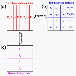
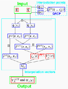
More specifically, we describe the various quantities in the ACE-ISDF method and the corresponding storage formats in Figure 3. Starting from and distributed in the column cyclic partition, we first transform these matrices into the 2D block cyclic partition to generate the matrix. We then perform the QRCP procedure to obtain the permutation matrix . The interpolation points are retrieved from the permutation matrix . This is a small vector of size , and are shared among all processors.
In order to construct the interpolation vectors, we distribute the columns of the quasi density matrices and in a 2D block cyclic fashion so that the matrix defined in (14) can be evaluated in parallel via local Hadamard multiplications. The matrix that appears in (13) can be obtained by simply subsampling rows of .
The resulting discretized interpolation vectors can be obtained by calling a ScaLAPACK linear equation solver. The 2D block cyclically distributed solution is redistributed and partitioned by a 1D column partition for computing the Coulomb-like potential for the interpolation vectors as in Eq. (18). are then converted back to the 2D block cyclic distribution pattern. Finally, the in Eq. (23) can be computed using matrix-matrix multiplication in the 2D partition as in Eq. (17), and then converted to 1D row partition.
In order to implement the symmetric formulation for the matrix in Eq. (27) as required by ACE, we form the matrix in Eq. (28) in parallel within a 2D block cyclic distribution scheme, and the matrix in Eq. (27) can be obtained by two parallel matrix-matrix multiplication calls. Finally, we perform a parallel Cholesky factorization of on the 2D block cyclic grid, and the ACE vectors are partitioned by rows on a 1D processor grid. This gives the implicitly, and can be readily used in subsequent iterations.
5 Numerical results
We demonstrate the performance of the ACE-ISDF method using the DGDFT (Discontinuous Galerkin Density Functional Theory) software package.[46, 47, 48, 49, 50] DGDFT is a massively parallel electronic structure software package designed for large scale DFT calculations involving up to tens of thousands of atoms. It includes a self-contained module called PWDFT for performing planewave based electronic structure calculations (mostly for benchmarking and validation purposes). We implemented the ACE-ISDF method in PWDFT. We use the Message Passing Interface (MPI) to handle data communication, and the Hartwigsen-Goedecker-Hutter (HGH) norm-conserving pseudopotential[51]. All calculations use the HSE06 functional.[7] All calculations are carried out on the Edison systems at the National Energy Research Scientific Computing Center (NERSC). Each node consists of two Intel “Ivy Bridge” processors with cores in total and 64 gigabyte (GB) of memory. Our implementation only uses MPI. The number of cores is equal to the number of MPI ranks used in the simulation.
In this section, we demonstrate the accuracy of the ACE-ISDF method for accelerating hybrid functional calculations, using a bulk silicon system Si216 and a disordered system Al176Si24[49] as shown in Figure 4 (a) and (b), respectively. The Si216 system is semiconducting with an energy gap of eV, and the Al176Si24 system is metallic with eV. The density of states of the two systems are shown in Figure 4 (c) and (d), respectively. All systems are closed shell systems, and the number of occupied bands is . We include two unoccupied bands for computing the energy gap in the systems. We show the parallel scalability of our implementation using 7 bulk silicon systems with to atoms.[31] Finally, we use the ACE-ISDF method in a hybrid DFT calculation to study the electronic structure of vacancy defect in a silicon supercell that contains Si atoms.
5.1 Accuracy
In the previous work,[30, 31] we demonstrated that the ACE formulation can significantly accelerate hybrid functional calculations without loss of accuracy. Hence the results from the ACE calculation is used as the baseline for comparison in assessing the accuracy of the ACE-ISDF method. Table 1 shows the convergence of the ACE-ISDF method as a function of the rank parameter for the Si216 and Al176Si24 systems. We measure the accuracy in terms of the valence band maximum (VBM) energy level, the conduction band minimum (CBM) energy levels, the energy gap, the Hartree-Fock (HF) exchange energy, the total energy as well as the atomic force. The energy cutoff is set to Hartree. We define the errors in the HF energy, the total energy and the atomic force respectively as
Here is the total number of atoms and is the atom index.

| ACE-ISDF: Semiconducting Si216 () | ||||||
| 4.0 | 6.5303 | 8.4367 | 1.9064 | 3.53E-03 | 4.13E-03 | 1.49E-03 |
| 5.0 | 6.5923 | 8.3652 | 1.7729 | 2.37E-03 | 2.75E-03 | 1.30E-03 |
| 6.0 | 6.6786 | 8.2535 | 1.5749 | 7.34E-04 | 1.06E-03 | 1.00E-03 |
| 7.0 | 6.6893 | 8.1554 | 1.4661 | 3.56E-04 | 4.61E-04 | 6.61E-04 |
| 8.0 | 6.6763 | 8.1341 | 1.4578 | 1.16E-04 | 1.64E-04 | 3.05E-04 |
| 9.0 | 6.6652 | 8.1164 | 1.4512 | 4.74E-05 | 7.50E-05 | 1.48E-04 |
| 10.0 | 6.6565 | 8.1085 | 1.4520 | 2.33E-05 | 4.11E-05 | 1.09E-04 |
| 12.0 | 6.6487 | 8.1001 | 1.4514 | 7.27E-06 | 1.54E-05 | 5.88E-05 |
| 16.0 | 6.6467 | 8.0959 | 1.4492 | 1.57E-06 | 2.92E-06 | 1.67E-05 |
| 20.0 | 6.6466 | 8.0942 | 1.4476 | 5.40E-07 | 7.87E-07 | 5.54E-06 |
| ACE | 6.6467 | 8.0934 | 1.4466 | 0.00E-00 | 0.00E-00 | 0.00E-00 |
| ACE-ISDF: Metallic Al176Si24 () | ||||||
| 4.0 | 7.8907 | 7.9963 | 0.1056 | 7.20E-03 | 8.06E-03 | 8.96E-03 |
| 5.0 | 7.8173 | 7.9103 | 0.0930 | 3.46E-03 | 3.76E-03 | 3.96E-03 |
| 6.0 | 7.7810 | 7.8833 | 0.1023 | 1.33E-03 | 1.69E-03 | 2.32E-03 |
| 7.0 | 7.7805 | 7.8742 | 0.0937 | 5.97E-04 | 6.41E-04 | 1.60E-03 |
| 8.0 | 7.7717 | 7.8710 | 0.0993 | 1.90E-04 | 2.03E-04 | 5.55E-04 |
| 9.0 | 7.7719 | 7.8710 | 0.0991 | 6.92E-05 | 7.44E-05 | 3.10E-04 |
| 10.0 | 7.7713 | 7.8699 | 0.0986 | 3.20E-05 | 3.55E-05 | 1.53E-04 |
| 12.0 | 7.7712 | 7.8695 | 0.0983 | 1.16E-05 | 1.38E-05 | 9.23E-05 |
| 16.0 | 7.7704 | 7.8698 | 0.0994 | 3.26E-06 | 4.43E-06 | 4.34E-05 |
| 20.0 | 7.7703 | 7.8695 | 0.0992 | 1.27E-06 | 1.93E-06 | 2.18E-05 |
| ACE | 7.7701 | 7.8695 | 0.0994 | 0.00E-00 | 0.00E-00 | 0.00E-00 |
Our calculations show that the ACE-ISDF method can produce highly accurate results with a moderate rank parameter . (Recall that the rank of the ISDF approximation is .) The accuracy of the approximation can be improved systematically by increasing the rank parameter . When a relatively small value (e.g., ) is used, the error in the total energy of both the Si216 and the Al176Si24 systems is already below that required to reach the chemical accuracy of 1 kcal/mol (1.6 Hartree/atom)[52]. For Si216, the errors in the HF energy, the total energy and the atomic force systematically decrease from to when is adjusted from 6.0 to 20.0. We note that the total energy convergence with respect to the rank parameter is similar between Si216 and Al176Si24. The fact that the rank parameter is independent of the band gap makes ISDF more attractive than linear scaling methods[53, 54, 55, 56] whose accuracy is controlled by the level of truncation in the density matrix, which in turn depends strongly on the band gap.
5.2 Efficiency
We demonstrate the efficiency of the ACE-ISDF method by showing its performance in a hybrid DFT calculation for a bulk silicon system with atoms ( = 2000) on cores. In each outer iteration, the cost of hybrid functional calculations consists of the cost for constructing the ACE operator (with or without ISDF) and the amount of work performed in the inner SCF iterations.
Table 2 shows the wall clock time spent in major components of the ACE-ISDF and ACE calculations, respectively. The main cost for constructing the ACE operator without using the ISDF decomposition is in the solution of Poisson-like equations via FFTs. For this silicon system, the number of Poisson-like equations to be solved in each outer iteration is as large as . To show the detailed cost of constructing the ACE operator using the ISDF method, we report the timing measurements for selecting the interpolation points (IP), computing the interpolation vectors (IV) and other linear algebra operations and FFTs (labeled by ‘Other’). The IP selection is performed once only in the first outer SCF iteration. Computing the IVs constitutes a major part of the cost in the construction of the ACE operator in subsequent outer SCF iterations. The time spent in solving Poisson equations using FFTs, which we list in the parenthesis next to time spent in the remaining parts of the ACE-ISDF calculation for comparison, is negligibly small. The reason that this cost is so small is that the use of ISDF significantly reduces the number of Poisson equations to be solved from to (when the rank parameter is set to 6.)
| Si1000 | ACE-ISDF | ACE | ||||||
|---|---|---|---|---|---|---|---|---|
| IP | IV | Other (FFT) | FFT | |||||
| 10 | 743 | 50.22 | 11.13 | 8.56 (0.28) | 101.10 | |||
| 20 | 1043 | 105.95 | 24.52 | 20.52 (1.17) | 148.73 | |||
| 30 | 1283 | 222.36 | 40.67 | 32.88 (1.31) | 302.98 | |||
| 40 | 1483 | 454.42 | 63.56 | 54.95 (3.08) | 807.31 | |||
When is set to 10 Hartree and is set to 6.0, the IP and IV computations take 50.22 s and 11.13 s respectively in ACE-ISDF. The total amount of time spent in the construction of the ACE operator via ISDF in the first SCF iteration, which is 70 s (50.22+11.13+8.56), is already lower than that used to construct the ACE operator without ISDF (a procedure dominated by solving a larger number of Poisson-like equations via FFTs), which is roughly 101.10 s. In each subsequent outer SCF iteration, a total of 19.86 s (11.13+8.56) are used to construct the ACE operator via ISDF. This is already comparable to the time of one SCF iteration in GGA calculations, which is s.
Note that for some complex systems, more inner SCF iterations might be required in each outer SCF iteration to reach convergence. For example, for the disordered Al176Si24 system, we need to use 14 inner SCF iterations per outer SCF iteration. As a result, the cost difference between ACE and ACE-ISDF is magnified, and ACE-ISDF is even more advantageous in these situation.
To illustrate the reduction of cost the ACE-ISDF scheme has achieved, we report that the average time spent in the construction and application of the exchange operator per outer SCF iteration in the conventional hybrid functional calculations is 1146.36 s, which is nearly two orders of magnitude higher than that used in ACE-ISDF. The large cost mainly comes from the fact that conventional hybrid functional calculations require solving Poisson like equations using FFTs in each step of an iterative diagonalization procedure (e.g. PPCG) when the exchange operator is applied to a set of orbitals. For this system, on average such operations need to be performed during each outer iteration. The ACE formulation reduces the cost by only requiring the exchange operator to be applied once per outer iteration, and the ACE-ISDF method further reduces the cost for this single application of the exchange operator.
As we discussed earlier, since IP calculation is significantly more expensive, it is important to perform such a calculation only once in order to make ACE-ISDF efficient. We found that the Hartree-Fock exchange energy obtained from using a fixed set of IPs throughout the SCF iteration differs only slightly from that obtained by recalculating IPs in each outer SCF iteration (dynamic IP) as shown in Table 3 for Si216 and Al176Si24. We can clearly see from the table that the difference between the first and the second columns is much smaller than the difference between the second and third columns. This shows that using fixed IP is well justified.
| Systems | fixed IP in ACE-ISDF | dynamic IP in ACE-ISDF | ACE | ||
|---|---|---|---|---|---|
| Si216 | -45.3225 | -45.3250 | -45.4835 | ||
| Al176Si24 | -25.9112 | -25.9093 | -26.1745 |
Hence in practice we only use the QRCP decomposition in the first outer SCF iteration to select IPs, whereas the update of the basis vectors is performed in each subsequent outer SCF iterations.
Table 2 also shows that, as is increased from 10 to 40 Hartree, the time spent in constructing the ACE operator increases from 101.10 s to 807.31 s. The time spent in identifying the interpolation points via QRCP also increases from 50.22 s to 454.42 s. However, the time used to compute the interpolation vectors only increases from 11.13 s to 63.56 s. Given that the interpolating points only need to be selected once, the performance gain achieved by ISDF is more notable at a larger value. This feature is particularly attractive for calculations that requiring large kinetic energy cutoff, such as those involving transition metal oxides.
5.3 Parallel scalability
To illustrate the strong parallel scalability of the ACE-ISDF method for large-scale hybrid DFT calculations, we report the change of the wallclock time in one outer SCF iteration with respect to the number of cores for the Si1000 system. The measured wallclock time includes time spent in one inner SCF iteration and in the ACE-ISDF operator construction. We also report the weak scaling of ACE-ISDF by showing the variation of the wallclock time with respect to the system size for a calculation that uses 8,192 cores. These results are given in Figure 5 which shows that our implementation of the ACE-ISDF method scales nearly perfectly up to 2,000 cores for the Si1000 system. It also shows ACE-ISDF scales well with respect to the system size (up to 4096 atoms) on 8192 cores.

5.4 Application to vacancy defect in silicon
Silicon is one of the most important materials in industry due to its remarkable properties and a wide range of applications in electronics. However, the presence of defects can significantly affect these properties. Furthermore, defects also can be extremely useful for designing innovative electronic devices.[57, 58] Therefore, accurate description of the electronic structures of silicon defects[59] is required to examine their effects on the electronic devices.
It is well known that DFT calculations based on LDA and GGA functionals are not reliable in predicting electronic structures of nanosystems.[60] In particular, such DFT calculations tend to underestimate the energy gap of semiconductors. For example, GGA calculations that use the PBE functional[13] give an energy gap of 0.69 eV in silicon, which is much smaller than that in bulk silicon measured in the experiments (1.17 eV)[61]. The use of hybrid functionals can mitigate this type of error.
The defect concentration in silicons used in experimental studies is about 1018 cm-3. To faithfully represent experimental conditions and avoid the nonphysical interactions between a defect and its images introduced by periodic boundary conditions, a large unit cell containing thousands of silicon atoms is required to in a computational study. Systems of this size is beyond the capability of existing planewave DFT software when a hybrid functional is used in the calculation. In this section we employ the ACE-ISDF method implemented in PWDFT to calculate the energy levels of a vacancy defect in an 1000-atom silicon system using the HSE06 hybrid functional. The defect concentration is about 5 1019 cm-3 in this case, which is close to concentration used in experimental studies. Our calculation based on the HSE06 functional yields an energy gap of 1.28 eV, which is very close to the experimental value of 1.17eV. We also find that a calculation that uses a smaller unit cell that contains 512 atoms yields an energy gap of 1.32 eV[31], and hence the size effect plays an important role.
Figure 6 shows the electronic structure of the vacancy defect in the Si1000 system computed with two different exchange-correlation functionals (GGA-PBE and HSE06). We fully relax the structures respectively with the GGA and HSE06 exchange-correlation functionals by using the steepest descent algorithm with the Barzilai-Borwein line search method [62] to optimize the geometry of the atomic configuration. The optimal unit cell lattice constants we obtained are 5.46 and 5.45 Å respectively for the GGA-PBE and HSE06 exchange-correlation functional based calculations. These values are close to those reported in previous theoretical studies.[63]
Our DFT calculations show that hybrid functional HSE06 calculations accurately describe the VBM and CBM energy levels of the silicon and the defect energy levels introduced by the vacancy defect. Furthermore, we can clearly see that the vacancy defect introduces three defect states into the intrinsic energy gap (1.28 eV) of silicon. These include a single defect state and a doubly degenerate state , 0.14 and 1.04 eV above the VBM energy of silicon, respectively. The GGA based DFT calculations fail to accurately predict these defect states.

6 Conclusion
In this paper, we demonstrate that the interpolative separable density fitting (ISDF) decomposition can be used to reduce the cost hybrid functional calculations for large systems in a planewave DFT code. The reduction in cost results from the construction of a set of numerical auxiliary basis vectors, where is a modest constant. Using these auxiliary basis vectors instead of products of the occupied orbitals, we only need to solve Poisson-like equations instead of equations to apply an approximate exchange operator to a set of occupied orbitals. The accuracy of the approximation depends entirely on the rank parameter , and we find that the choice of is insensitive with respect to the band gap.
The ISDF decomposition can be performed in operations. The interpolation points are chosen by a randomized QR factorization with column pivoting (QRCP). It is relatively expensive compared to other parts of the ISDF calculation. However, this procedure only needs to be carried out once for all during the first outer SCF iteration in a hybrid functional calculation. The interpolation vectors can be computed via a least squares fitting procedure that makes use of the separable nature of the functions to be fitted. The complexity of this step still scales as but with a significantly smaller preconstant compared to the cost of applying the uncompressed exchange operator or the cost of QRCP. We are currently also exploring other methods for selecting interpolation points that avoid the use of the QRCP procedure, especially in the context of geometry optimization and ab initio molecular dynamics simulation.
For a moderate choice of rank parameter, the error in the total energy per atom and the force can be kept under Hartree/atom and Hartree/Bohr respectively, for both semiconducting and metallic systems. Meanwhile the computational time can be reduced by up to an order of magnitude for applying the exchange operator once to all Kohn-Sham orbitals. We demonstrated that the ISDF decomposition can be combined with the adaptively compressed exchange operator (ACE) formulation to reduce the cost of ACE operator construction. The resulting ACE-ISDF method exhibits excellent parallel scalability on high performance computers, and significantly reduces the time required to perform hybrid functional calculations by nearly two orders of magnitude. In particular, the time spent in ACE-ISDF enabled hybrid functional calculation is only marginally higher than that spent in DFT calculations that use local and semilocal functionals.
However, we also find that hybrid functionals calculations often require more iterations to converge compared to GGA calculations. One main reason is the two level SCF iteration structure in hybrid functional calculations, which may be inefficient especially in the context of ab initio molecular dynamics simulation. Further reduction of the number of SCF iterations may close the final gap between hybrid functional calculations and calculations with local and semilocal functionals, and thus opens the door to the accurate simulation of a vast range of nanomaterials using hybrid functionals beyond reach today.
7 Acknowledgments
This work was partly supported by the Scientific Discovery through Advanced Computing (SciDAC) program funded by U.S. Department of Energy, Office of Science, Advanced Scientific Computing Research and Basic Energy Sciences (W. H., L. L. and C. Y.), by the National Science Foundation under grant DMS-1652330 (L. L.), and by the Center for Applied Mathematics for Energy Research Applications (CAMERA) (L. L. and C. Y.). The authors thank the National Energy Research Scientific Computing (NERSC) center and the Berkeley Research Computing program at the University of California, Berkeley for making computational resources available to them. We would like to thank Francois Gygi, Jianfeng Lu, Meiyue Shao and Lexing Ying for helpful discussions.
References
- (1) Hohenberg, P.; Kohn, W. Phys. Rev. 1964, 136, B864.
- (2) Kohn, W.; Sham, L. J. Phys. Rev. 1965, 140, A1133.
- (3) Perdew, J. P.; Schmidt, K. AIP Conference Proceedings 2001, 577, 1.
- (4) Becke, A. D. J. Chem. Phys. 1993, 98, 1372.
- (5) Perdew, J. P.; Ernzerhof, M.; Burke, K. J. Chem. Phys. 1996, 105, 9982.
- (6) Heyd, J.; Scuseria, G. E.; Ernzerhof, M. J. Chem. Phys. 2003, 118, 8207.
- (7) Heyd, J.; Scuseria, G. E.; Ernzerhof, M. J. Chem. Phys. 2006, 124, 219906.
- (8) Ceperley, D. M.; Alder, B. J. Phys. Rev. Lett. 1980, 45, 566.
- (9) Perdew, J. P.; Zunger, A. Phys. Rev. B 1981, 23, 5048.
- (10) Goedecker, S.; Teter, M.; Hutter, J. Phys. Rev. B 1996, 54, 1703.
- (11) Becke, A. D. Phys. Rev. A 1988, 38, 3098.
- (12) Lee, C.; Yang, W.; Parr, R. G. Phys. Rev. B 37, 785 1988, 37, 785.
- (13) Perdew, J. P.; Burke, K.; Ernzerhof, M. Phys. Rev. Lett. 1996, 77, 3865.
- (14) Tao, J.; Perdew, J. P.; Staroverov, V. N.; Scuseria, G. E. Phys. Rev. Lett. 2003, 91, 146401.
- (15) Sun, J.; Ruzsinszky, A.; Perdew, J. P. Phys. Rev. Lett. 2015, 115, 036402.
- (16) Sun, J.; Perdew, J. P.; Ruzsinszky, A. Proc. Natl. Acad. Sci. USA 2015, 112, 685–689.
- (17) Duchemin, I.; Gygi, F. Comput. Phys. Commun. 2010, 181, 855–860.
- (18) Bylaska, E. J.; Tsemekhman, K.; Baden, S. B.; Weare, J. H.; Jonsson, H. J. Comput. Chem. 2011, 32, 54–69.
- (19) Barnes, T. A.; Kurth, T.; Carrier, P.; Wichmann, N.; Prendergastc, D.; Kent, P. R. C.; Deslippe, J. Comput. Phys. Commun. 2017, 214, 52–58.
- (20) Goedecker, S. Rev. Mod. Phys. 1999, 71, 1085.
- (21) Bowler, D. R.; Miyazaki, T. Rep. Prog. Phys. 2012, 75, 036503.
- (22) Guidon, M.; Hutter, J.; VandeVondele, J. J. Chem. Theory Comput. 2010, 6, 2348–2364.
- (23) DiStasio, R. A.; Jr.,; Santra, B.; Li, Z.; Wu, X.; Car, R. J. Chem. Phys. 2014, 141, 084502.
- (24) Dawson, W.; Gygi, F. J. Chem. Theory Comput. 2013, 11, 4655–4663.
- (25) Damle, A.; Lin, L.; Ying, L. J. Chem. Theory Comput. 2015, 11, 1463–1469.
- (26) Kohn, W. Phys. Rev. Lett. 1996, 76, 3168.
- (27) Rebolini, E.; Izsák, R.; Reine, S. S.; Helgaker, T.; Pedersen, T. B. J. Chem. Theory Comput. 2010, 12, 3514–3522.
- (28) Manzer, S.; Horn, P. R.; Mardirossian, N.; Head-Gordon, M. J. Chem. Phys. 2015, 143, 024113.
- (29) Boffi, N. M.; Jain, M.; Natan, A. J. Chem. Theory Comput. 2016, 12, 3614–3622.
- (30) Lin, L. J. Chem. Theory Comput. 2016, 12, 2242–2249.
- (31) Hu, W.; Lin, L.; Banerjee, A. S.; Vecharynski, E.; Yang, C. J. Chem. Theory Comput. 2017, 13, 1188–1198.
- (32) Lin, L.; Lindsey, M. arXiv:1703.05441 2017, .
- (33) Giannozzi, P. et al. J. Phys.: Condens. Matter 2009, 21, 395502.
- (34) Lu, J.; Ying, L. J. Comput. Phys. 2015, 302, 329–335.
- (35) Manzer, S.; Horn, P. R.; Mardirossian, N.; Head-Gordon, M. J. Chem. Phys. 2015, 143, 024113.
- (36) Ren, X.; Rinke, P.; Blum, V.; Wieferink, J.; Tkatchenko, A.; Sanfilippo, A.; Reuter, K.; Scheffler, M. New J. Phys. 2012, 14, 053020.
- (37) Weigend, F. Phys. Chem. Chem. Phys. 2002, 4, 4285–4291.
- (38) Parrish, R. M.; Hohenstein, E. G.; Martínez, T. J.; Sherrill, C. D. J. Chem. Phys. 2012, 137, 224106.
- (39) Parrish, R. M.; Hohenstein, E. G.; Martínez, T. J.; Sherrill, C. D. J. Chem. Phys. 2013, 138, 194107.
- (40) Golub, G. H.; Reinsch, C. Numerische Mathematik 1970, 14, 403–420.
- (41) Harbrecht, H.; Peters, M.; Schneider, R. Applied Numerical Mathematics 2012, 62, 428–440.
- (42) Chan, T. F.; Hansen, P. C. SIAM J. Sci. Statist. Comput. 1992, 13, 727–741.
- (43) Freysoldt, C.; Grabowski, B.; Hickel, T.; Neugebauer, J.; Kresse, G.; Janotti, A.; de Walle, C. G. V. Proc. Natl. Acad. Sci. USA 2007, 104, 20167–20172.
- (44) Halko, N.; Martinsson, P. G.; Tropp, J. A. SIAM Rev. 2011, 53, 217–288.
- (45) Auckenthaler, T.; Blum, V.; Bungartz, H. J.; Huckle, T.; Johanni, R.; Krämer, L.; Lang, B.; Lederer, H.; Willems, P. R. Parallel Comput. 2011, 37, 783-794.
- (46) Lin, L.; Lu, J.; Ying, L.; E, W. J. Comput. Phys. 2012, 231, 2140-2154.
- (47) Hu, W.; Lin, L.; Yang, C. J. Chem. Phys. 2015, 143, 124110.
- (48) Hu, W.; Lin, L.; Yang, C. Phys. Chem. Chem. Phys. 2015, 17, 31397–31404.
- (49) Banerjee, A. S.; Lin, L.; Hu, W.; Yang, C.; Pask, J. E. J. Chem. Phys. 2016, 145, 154101.
- (50) Zhang, G.; Lin, L.; Hu, W.; Yang, C.; Pask, J. E. J. Comput. Phys. 2017, 335, 426–443.
- (51) Hartwigsen, C.; Goedecker, S.; Hutter, J. Phys. Rev. B 1998, 58, 3641.
- (52) Pople, J. A. Rev. Mod. Phys. 1999, 71, 1267.
- (53) Schwegler, E.; Challacombe, M. J. Chem. Phys. 1996, 105, 2726.
- (54) Ochsenfeld, C.; White, C. A.; Head-Gordon, M. J. Chem. Phys. 1998, 109, 1663.
- (55) Shang, H.; Li, Z.; Yang, J. J. Chem. Phys. 2011, 135, 034110.
- (56) Shang, H.; Li, Z.; Yang, J. J. Phys. Chem. A 2010, 114, 1039–1043.
- (57) Newman, R. C. Rep. Prog. Phys. 1982, 45, 1163.
- (58) Watkins, G. D. Mater. Sci. Semicond. Process. 2000, 3, 227.
- (59) Freysoldt, C.; Grabowski, B.; Hickel, T.; Neugebauer, J.; Kresse, G.; Janotti, A.; de Walle, C. G. V. Rev. Mod. Phys. 2014, 86, 253.
- (60) Heyd, J.; Peralta, J. E.; Scuseria, G. E.; Martin, R. L. J. Chem. Phys. 2005, 123, 174101.
- (61) Ledoux, G.; Gong, J.; Huisken, F. Appl. Phys. Lett. 2002, 80, 4834.
- (62) Barzilai, J.; Borwein, J. M. IMA J. Numer. Anal. 1988, 8, 141–148.
- (63) Lucero, M. J.; Henderson, T. M.; Scuseria, G. E. J. Phys.: Condens. Matter 2012, 24, 145504.
![[Uncaptioned image]](1707.09141v1/TOC.png) |
TOC graphic