P-splines with an penalty for repeated measures
P-splines are penalized B-splines, in which finite order differences in coefficients are typically penalized with an norm. P-splines can be used for semiparametric regression and can include random effects to account for within-subject variability. In addition to penalties, -type penalties have been used in nonparametric and semiparametric regression to achieve greater flexibility, such as in locally adaptive regression splines, trend filtering, and the fused lasso additive model. However, there has been less focus on using penalties in P-splines, particularly for estimating conditional means.
In this paper, we demonstrate the potential benefits of using an penalty in P-splines with an emphasis on fitting non-smooth functions. We propose an estimation procedure using the alternating direction method of multipliers and cross validation, and provide degrees of freedom and approximate confidence bands based on a ridge approximation to the penalized fit. We also demonstrate potential uses through simulations and an application to electrodermal activity data collected as part of a stress study.
1 Introduction
Many nonparametric regression methods, including smoothing splines and regression splines, obtain point estimates by minimizing a penalized negative log-likelihood function of the form , where is a log-likelihood, is a penalty term, is a smoothing parameter, and are the coefficients to be estimated. Typically, quadratic ( norm) penalties are used, which lead to straightforward computation and inference. In particular, penalties typically lead to ridge estimators, which have both closed form solutions and are linear smoothers. The penalty also has connections to mixed models, which allows the smoothing parameters to be estimated as variance components (Green,, 1987; Speed,, 1991; Wang,, 1998; Zhang et al.,, 1998).
However, nonparametric regression methods that use an -type penalty, such as trend filtering (Kim et al.,, 2009) and locally adaptive regression splines (Mammen et al.,, 1997), are better able to adapt to local differences in smoothness and achieve the minimax rate of convergence for weakly differentiable functions of bounded variation (Tibshirani, 2014a, ), whereas penalized methods do not (Donoho and Johnstone,, 1988). The trade-off is that penalties generally lead to more difficult computation and inference because the objective function is convex but non-differentiable, and the fit is no longer a linear smoother.
In this article, we propose P-splines with an penalty as a framework for generalizing trend filtering within the context of repeated measures data and semiparametric (additive) models (Hastie and Tibshirani,, 1986). In Section 2, we discuss the connection between P-splines and trend filtering which motivates the methodological development. In Section 3, we present our proposed model, and in Section 4, we discuss related work. In Section 5, we propose an estimation procedure using the alternating direction method of multipliers (ADMM) (Boyd et al.,, 2011, see) and cross validation (CV). In Section 6, we derive the degrees of freedom and propose computationally stable and fast approximations, and in Section 7, we develop approximate confidence bands based on a ridge approximation to the fit. In Section 8, we study our method through simulations and evaluate its performance in fitting non-smooth functions. In section 9, we demonstrate our method in an application to electrodermal activity data collected as part of a stress study. We close with a discussion in Section 10.
2 P-splines and trend filtering
In this section, we give brief background on P-splines and trend filtering, and show the relation between them when the data are independent and identically distributed (i.i.d.) normal.
P-splines (Eilers and Marx,, 1996) are penalized B-splines (De Boor,, 2001, see). B-splines are flexible bases that are notable in part because they have compact support, which leads to banded design matrices and faster computation. This compact support can be seen in Figure 1, which shows eight evenly spaced first degree and third degree B-spline bases on . We can define an order (degree ) B-spline basis with basis functions recursively as (De Boor,, 2001)
where are the knots, division by zero is taken to be zero, and is the number of internal knots. For order B-splines defined on the interval , in order to obtain basis functions, we set boundary knots ( knots on each side) and interior knots. In general, one can set . In order to ensure continuity at the boundaries, we set and . We also use equally spaced interior knots, which is important for the P-spline penalty, and drop the superscript on designating order when the order does not matter or is stated in the text.

B-spline bases can be used to fit nonparametric models of the form , where is the outcome at point , is the mean response function at , and is the error at . To that end, let be an vector of outcomes and be a corresponding vector of covariates. Also, let be B-spline basis functions and let be an design matrix such that , i.e., the column of is the basis function evaluated at . Equivalently, the row of is the data point evaluated by . For i.i.d. normal , a simple linear P-spline model with the standard penalty can be written as
| (1) |
where is the intercept, is a vector of parameter estimates, is an vector with each element equal to 1, is a smoothing parameter, and is the order finite difference matrix. For example, for
| (2) |
In general, as described by Tibshirani, 2014a (), where is the upper left matrix of:
| (3) |
Our proposed model builds on one in which the penalty in (1) is replaced with an penalty:
| (4) |
Letting , for order B-splines, Eilers and Marx, (1996) show that
where is the second-order backwards difference and and are constants. As shown in Appendix C, a similar result holds for P-splines with an penalty. In particular, for ,
where is a constant given in Appendix C that depends on the order of the B-splines and order of the finite difference. In other words, controlling the norm of the order finite differences in coefficients also controls the total variation of the derivative of the function.
trend filtering is similar to (4). In the case where are unique and equally spaced, trend filtering solves the following problem (the intercept is handled implicitly):
| (5) |
Problem (5) differs from (4) in that (5) has one parameter per data point, and the design matrix is the identity matrix. is also resized appropriately by replacing with in the dimensions of (2) and (3). However, under certain conditions noted in Observation 1, (4) and (5) are identical.
Observation 1 (Continuous representation).
For second order (first degree) B-splines with basis functions, equally spaced data with knots at , and centered outcomes such that , P-splines with an penalty are a continuous analogue to trend filtering.
Proof of Observation 1.
Under these conditions, for
To see this, note that
| (6) |
Now,
We have for and otherwise, but for , we have . We also have for and 0 otherwise, and for , we have . It follows that for , (6) evaluates to 1 if and 0 otherwise.
We note that Tibshirani, 2014a () shows that trend filtering has a continuous representation when expressed in the standard lasso form, and Observation 1 gives a continuous representation of trend filtering when expressed in generalized lasso form.
trend filtering can be applied to irregularly spaced data, such as with the algorithm developed by Ramdas and Tibshirani, (2016). It might also be possible to extend trend filtering to repeated measures data to account for within-subject correlations. However, due to Observation 1, we think it is beneficial to view trend filtering as a special case of P-splines with an penalty. We think this approach has the potential to be a general framework, because higher order B-splines could be used in combination with different order difference matrices just as can be done with P-splines that use the standard penalty. Furthermore, expressing trend filtering as P-splines with an penalty may facilitate the development of confidence bands (see Section 7), which could help to fill a gap in the penalized regression literature.
In addition, there are connections between P-splines with an penalty and locally adaptive regression splines. In particular, as Tibshirani, 2014a () shows, the continuous analogue of trend filtering is identical to locally adaptive regression splines (Mammen et al.,, 1997) for , and asymptotically equivalent for .
3 Proposed model: additive mixed model using P-splines with an penalty
To introduce our model, let be an vector of responses for subject , and let be the stacked vector of responses for all subjects, where . Let be a corresponding vector of covariates for subject , and be the stacked vector of all covariate values. In many contexts, is time. To account for the within-subject correlations of , we can incorporate random effects into the P-spline model. To that end, let be an design matrix for the random effects for subject (possibly including a B-spline basis), and let be the corresponding vector of random effect coefficients for subject . Also, let
be the block diagonal random effects design matrix for all subjects, where , and let be the stacked vector of random effects for all subjects. We propose an additive mixed model with smooths (tildes denote quantities that will be subject to additional constraints, as described below):
| (7) |
where is a design matrix of B-spline bases for smooth , is the finite difference matrix, and is the covariance matrix of the random effects . For example, if are random intercepts, then and would be an matrix such that if observation belonged to subject and zero otherwise. Alternatively, to obtain random curves using smoothing splines and a B-spline basis, we could set
where , and are the second derivatives of the B-spline basis functions for the smooth. We would then set to be the corresponding B-splines evaluated at the input points.
We note that (7) includes varying-coefficient models (Hastie and Tibshirani,, 1993). For example, as pointed out by Wood, (2006, p. 169), if are B-splines evaluated at , we could have , where is another covariate vector and is a diagonal matrix with at the leading diagonal position.
As written, (7) is not generally identifiable. To see this, suppose , where neither nor are varying-coefficient terms. Then letting and for , we also have . To make (7) identifiable, we follow Wood, (2006, Section 4.2) and introduce a centering constraint on each non-varying coefficient smooth, i.e. for all smooths such that for some and . To this end, let be the indices of the non-varying coefficient smooths, and let be its complement. We constrain for . We accomplish this by defining new orthonormal matrices , , such that . If desired, one can also define a matrix such that . However, this last centering constraint is not necessary, because the penalty on the random effect terms pulls the coefficients themselves towards zero, as opposed to the finite order differences in coefficients.
As Wood, (2006, Section 1.8.1) shows, can be obtained by taking the QR decomposition of and retaining the last columns of the left orthonormal matrix.11
1
The matrices , are of rank 1, so the remaining columns are arbitrary orthonormal vectors. In R (R Core Team,, 2017), when taking the QR decomposition of , an appropriate matrix can be obtained as Q ¡- qr.Q(qr(colSums(F_tilde)), complete = TRUE)[, -1]—. We can then re-parameterize the constrained parameters in terms of the unconstrained parameters , such that . For , let and . For , let and . If centering the random effects, then we redefine and . Then we can re-write (7) in the identifiable form
| (8) |
where for and for .
We note that the penalty matrix given above for random subject-specific splines defines non-zero correlation between nearby within-subject random effect coefficients. This is in contrast to the approach of Ruppert et al., (2003) for estimating subject-specific random curves, which focuses on the case in which nearby within-subject coefficients are not correlated. To see this, let be the estimated difference between the subject-specific curve and the marginal mean at point . The smoothing spline approach above constrains for some constant , whereas the approach of Ruppert et al., (2003) constrains . Whereas the non-diagonal penalty matrix implies correlations between nearby coefficients, the identity matrix in the approach of Ruppert et al., (2003) implies zero correlation.
Similar to the equivalence between Bayesian models and penalized smoothing splines (Wahba,, 1990), there is an equivalence between Bayesian models and penalized splines. In particular, (8) is equivalent to the following distributional assumptions, which we can use to obtain Bayesian estimates:
| (9) | ||||
The last distributional assumption is an element-wise Laplace prior on the order differences in coefficients.
In some cases, the random effects penalty matrix may be positive semidefinite but not invertible. For example, the smoothing spline random curves outlined above lead to a penalty matrix that is not strictly positive definite, but that is still positive semidefinite. This does not cause problems for the ADMM algorithm, but some changes are required for other algorithms as well as for Bayesian estimation. Following Wood, (2006, Section 6.6.1), let be the eigendecomposition of a positive semidefinite matrix , where and is a diagonal matrix with eigenvalues in descending order in the diagonal positions. Let and , so that and . Let be the number of strictly positive eigenvalues of , where , and let be the upper left portion of . We can partition as , where is a vector of penalized coefficients and is a vector of unpenalized coefficients, where . Then , and it follows that and .
However, allowing for unconstrained random effect parameters leads to identifiability issues. Therefore, in practice if , we recommend using a normal or Cauchy prior on . In particular, or , with either a diffuse prior on and constraints to ensure , or a diffuse prior on without constraints. The Cauchy prior may be a preferable first choice, as it provides a weaker penalty and is similar to the recommendations of Gelman et al., (2008) for logistic regression. However, in some cases, such as in Section 9, it is necessary to use a normal prior.
To further improve the computational efficiency of Monte Carlo sampling methods, we can partition into where contains the first columns of and contains the remaining columns. We then set and , so that and , which allows for more efficient sampling (Wood,, 2006).
4 Related work
There are many nonparametric and semiparametric methods for analyzing repeated measures data. For an overview, please see Fitzmaurice et al., (2008, Part III). However, most existing methods use an penalty (Rice and Wu,, 2001; Guo,, 2002; Chen and Wang,, 2011; Scheipl et al.,, 2015, e.g.).
Focusing on the optimization problem, our method puts a generalized lasso penalty (Tibshirani,, 1996) on the fixed effects and a quadratic penalty on the random effects. Unlike the elastic net (Zou and Hastie,, 2005), we do not mix the and penalties on the same parameters, though this could be done in the future.
The additive model with trend filtering developed by Sadhanala and Tibshirani, (2017) is similar to our approach. Sadhanala and Tibshirani, (2017) optimize
| (10) | ||||
In contrast to (8), (10) has one smoothing parameter and constrains all smooths to be zero-centered. From Observation 1, we see that (10) is equivalent to (8) when there are is smooth and no random effects, in which case there would be only one smoothing parameter and no varying-coefficient smooths.
Sadhanala and Tibshirani, (2017) develop the theoretical and computational aspects of additive models with trend filtering, including the extension of the falling factorial basis to additive models. Similar to the B-spline basis, the falling factorial basis allows for linear time multiplication and inversion, which leads to fast computation (Wang et al.,, 2014).
When smooths are expected to have similar degrees of freedom and is not large enough to require dimension reduction, then (10) with the addition of random effects and the relaxation of the zero-constraints for varying-coefficient smooths may be a viable alternative to (8) that could potentially adapt better to local differences in smoothness because it would have one knot per data point.
While not developed for analyzing repeated measures, the fused lasso additive model (FLAM) (Petersen et al.,, 2016) is also similar to (8). FLAM optimizes the following problem:
| (11) |
where specifies the balance between fitting piecewise constant functions () and inducing sparsity on the selected smooths (). From Observation 1, we see that (11) is equivalent to our model (8) when: , there is smooth, our design matrix has columns, our B-spline bases have appropriately chosen knots, and our model has no random effects. As Petersen et al., (2016) show, FLAM can be a very useful method for modeling additive phenomenon, and as with the fused lasso (Tibshirani et al.,, 2005), jumps in the piecewise linear fits have the advantage of being interpretable.
We also mention the sparse additive model (SpAM) (Ravikumar et al.,, 2009) and sparse partially linear additive model (SPLAM) (Lou et al.,, 2016). SpAM fits an additive model and uses a group lasso penalty (Yuan and Lin,, 2006) to induce sparsity on the number of active smooths. SPLAM fits a partially linear additive model and uses a hierarchical group lasso penalty (Zhao et al.,, 2009) to induce sparsity in the selected predictors and to control the number of nonlinear features.
One notable difference between our model and that of Sadhanala and Tibshirani, (2017), as well as FLAM, SpAM, and SPLAM, is that we allow for multiple smoothing parameters. In our applied experience with additive models and standard penalties, we have found that in practice it can be important to allow for multiple smoothing parameters, particularly when the quantities of interest are the individual smooths as opposed to the overall prediction. This is equivalent to allowing each smooth to have different variance. However, this flexibility comes at a cost: estimating multiple smoothing parameters is currently the greatest challenge in fitting our proposed model. Perhaps due in part to these computational difficulties, several other authors also assume a single smoothing parameter in high-dimensional additive models (Lin et al.,, 2006; Meier et al.,, 2009, e.g.).
There are fast and stable methods for fitting multiple smoothing parameters for penalties paired with exponential family and quasilikelihood loss functions, notably the work of Wood, (2004) using generalized cross validation (GCV) and Wood, (2011) using restricted maximum likelihood. Furthermore, Wood et al., (2015) extend these methods to larger datasets, and Wood et al., (2016) extend these methods to likelihoods outside the exponential family and quasilikelihood form. However, similarly computationally efficient methods do not yet exist for fitting multiple smoothing parameters for penalties.
In addition to allowing for multiple smoothing parameters, we also propose approximate inferential methods, which is not typically provided for penalized models. Yuan and Lin, (2006), Ravikumar et al., (2009), Lou et al., (2016), and Petersen et al., (2016) focus on prediction and provide bounds on the prediction risk and related quantities. These are important results, and we think that distributional results for individual parameters and smooths will also be useful to practitioners.
We also note that Eilers, (2000) and Bollaerts et al., (2006) discuss a variant of P-splines for quantile regression, in which the norm is used in both the loss and penalty function. However, we are not aware of existing P-spline methods that combine an penalty with an loss function.
5 Point estimation
5.1 Regression parameters and random effects
To fit (8), we use the alternating direction method of multipliers (ADMM) (Boyd et al.,, 2011, see). ADMM has the advantage of being scalable to large datasets. To formulate (8) for ADMM, we introduce constraint terms and re-write the optimization problem as
| minimize | (12) | |||
| subject to |
The augmented Lagrangian in scaled form (using to denote the scaled dual variable) is
where is the penalty parameter. The dimensions are , , , , , , , , , and , where if (non-varying coefficient smooths) and if (varying coefficient smooths).
ADMM is an iterative algorithm, and we re-estimate the parameters for updates until convergence.22 2 We use to denote the iteration of the ADMM algorithm. This is unrelated to our use of in Section 2 to denote the order of the B-spline basis. It is straightforward to derive the updates (see Boyd et al.,, 2011, Section 6.4.1):
| (13) | ||||
where and is the element-wise soft thresholding operator, where for a single scalar element
To initialize the algorithm, we set , , and , , and , for
As an alternative to the closed-form update (13) for the random effects, it is also possible to update the random effects via a linear mixed effects (LME) model that is embedded into the ADMM algorithm. In particular, an LME model is fit to the residuals , and are updated as the best linear unbiased predictors (BLUPs). This update occurs at each step of the ADMM algorithm and replaces the update given by (13). The LME update has the additional benefit of simultaneously estimating the variance of the random effects . In simulations, we have found that using an LME update leads to more accurate estimates of , which is important for subsequent estimates of degrees of freedom and confidence intervals.
For stopping criteria, we use the primal and dual residuals ( and , respectively):
where , , and is the cardinality of .
Following the guidance of Boyd et al., (2011), we stop when and , where
By default, we set and the maximum number of iterations at .
5.2 Smoothing parameters
To estimate we compute cross validation (CV) error for a path of values one smoothing parameter at a time. In the CV, we split the sample at the subject level, as opposed to individual observations, and ensure that there are at least two subjects in each fold per unique combination of factor covariates. First, we estimate a path for with set to 0. Then we fix at the value that minimizes CV error and compute a path for , setting it to the value that minimizes CV error, and so on.
We fit a path for each from to evenly spaced on the log scale, where is the smallest value at which . As shown in Appendix B,
, where are the partial residuals and for a vector , .
We also use warm starts, passing starting values separately for each fold, though warm starts appear to be minimally beneficial with ADMM. We set at each iteration for some constant (e.g. ). When the number of smooths is small (e.g. ) a grid search is also feasible.
To estimate , we can either use CV and the close-form update given by (13), or an LME update that is embedded in the ADMM algorithm, as described in Section 5.1. In simulations, we have found that the overall computation time to estimate the smoothing parameters is greater when using the LME update, and that the estimates of do not appear sensitive to updates for . However, the final estimates of , and consequently the width of confidence intervals can be improved by using the LME update. Consequently, we recommend using cross validation to estimate for the purposes of then estimating , but using an LME update when estimating the final model.
With both the closed-form and LME update, we cannot use the training sample to estimate the random effect parameters for the test sample, because these parameters are subject-specific and the test subjects are not included in the training sample. Instead, we use the training sample to obtain estimates for the fixed effect parameters , , and then use the test sample to estimate the random effects.
To make our approach clear, we first fix notation. Let be the row indices for the observations in the test sample for both the fixed and random effect design matrices , , and . Also, let be the column indices of for observations in the test sample, and let be the tuple of row and column indices designating the test sample. Let matrices and be matrix with only rows indexed by retained and removed, respectively. Similarly, let matrices and be matrix with only rows and columns indexed by and , respectively, retained and removed, respectively. Let matrices and be matrix with only rows and columns indexed by retained and removed, respectively. Also, let and be vector with elements indexed by retained and removed, respectively.
We obtain out-of-sample marginal estimates as , where and , are estimated with , , and . If using the closed-form update (13), we estimate subject-specific random effects as and obtain the out-of-sample prediction residuals as . Letting be the tuple of indices for test sample (fold) , we obtain the CV error as .
6 Degrees of freedom
In this section, we obtain the degrees of freedom, with the primary goal of estimating variance (see Section 7.1). However, we note that degrees of freedom does not always align with a model’s complexity in terms of its tendency to overfit the data (Janson et al.,, 2015).
In each of the approaches described in this section, the degrees of freedom (df) is a function of the smoothing parameters and . We always obtain the fixed effects smoothing parameters from CV, but when using an LME update for the random effects as described in Sections 5.1 and 5.2, we do not directly obtain . Consequently, we cannot directly apply the results in this section to estimate df. However, from (9), we have that . Writing , and letting be an vector of residuals and be an estimate of variance, we have that
Therefore, letting
we numerically solve for such that and set .
6.1 Stein’s method
Let , where is the model fitting procedure. For , the degrees of freedom is defined as (Efron,, 1986; Hastie and Tibshirani,, 1990, see)
| (14) |
As Tibshirani, 2014a () notes, (14) is motivated by the fact that the risk can be decomposed as
Therefore, the degrees of freedom (14) corresponds to the difference between risk and expected training error. Furthermore, if is continuous and weakly differentiable, then (Stein,, 1981) where is the divergence of . Therefore, an unbiased estimate of df (also used in Stein’s unbiased risk estimate (Stein,, 1981)) is
| (15) |
To obtain an estimate of degrees of freedom, we transform the generalized lasso component of our model to standard form, similar to the approach of Petersen et al., (2016). To do so, we use the following matrices described by Tibshirani, 2014b (). Let
be an augmented finite difference matrix, where is the first row of the finite difference matrix , and is the identity matrix. As shown by Tibshirani, 2014b (), the inverse of is given by where33 3 We denote the inverse matrix as . This is unrelated to our use of in Section 2 to denote the order of the B-spline basis.
where is the lower diagonal matrix of 1s.
Assuming our outcome is centered, so that , and letting , for and for , and , we can write the penalized log likelihood (8) as
| (16) |
To avoid difficulties later differentiating with respect to the norm, we remove the non-active penalized coefficients from (16). We also form the concatenated design matrix and will need to index the active set of . To these ends, let be the active set of the penalized coefficients for smooth , and let be the active set for smooth augmented with the unpenalized coefficients. Also, for a set and constant , let be the set of elements in shifted by . Now let be the augmented active set of , where and are the number of columns in (equivalently ). Finally, let be matrix subset to retain only those columns indexed by . Similarly, let be the concatenated vector of estimated coefficients, and let be vector subset to retain only elements indexed by . Then we can write the estimated penalized loss (16) as
| (17) |
Taking the derivative of (17) and keeping in mind that the first elements of each are unpenalized and for all , we have
| (18) |
where
is a vector of zeros, and the sign operator is taken element-wise.
From Tibshirani and Taylor, (2012, Lemmas 6 and 9), we know that within a small neighborhood of , the active set and the sign of the fitted terms are constant with respect to except for in a set of measure zero. Therefore, , where is an matrix of zeros and is the cardinality of . Then taking the derivative of (18) with respect to , we have
Solving for the derivatives of the estimated coefficients, we have
Now let and
Then since we have
From Tibshirani and Taylor, (2012, Lemmas 1 and 8), we know that is continuous and weakly differentiable. Also, . Therefore, we can use Stein’s formula (15) to estimate the degrees of freedom as
| (19) |
where we add 1 for the intercept. We note that this result is similar to the degrees of freedom for the elastic net (Tibshirani and Taylor,, 2012, see the remark on page 18 of) as well as for FLAM (Petersen et al.,, 2016).
To obtain degrees of freedom for individual smooths , let be an matrix with 1s on the diagonal positions indexed by and zero elsewhere, where is the cardinality of and . Also, let be the estimate of the smooth. Then as Ruppert et al., (2003) note, . Therefore,
| (20) |
In other words, the degrees of freedom for smooth is the sum of the diagonal elements of indexed by .
We note that when using the ADMM algorithm, or most likely any proximal algorithm, the fitted , or equivalently , will typically have several very small non-zero values, but will not typically be sparse. However, the vector is sparse, where in the ADMM algorithm we constrain . Therefore, in practice we use to obtain the active set .
6.2 Stable and fast approximations
In some cases, such as the application in Section 9, the estimates based on Stein’s method (19) and (20) cannot be computed due to numerical instability. In this section, we propose alternatives that are more numerically stable and which are also more computationally efficient.
6.2.1 Based on restricted derivatives
In this approach, we take derivatives of the fitted values restricted to individual smooths. In particular, from Section 6.1, we see that
We can then approximate the degrees of freedom for each individual smooth and the random effects by
| (21) |
We estimate the overall degrees of freedom as
| (22) |
where we add 1 for the intercept.
This approach is similar to one described by Ruppert et al., (2003, p. 176), though in a different context and for a different purpose. In particular, whereas we use this approach to approximate the degrees of freedom after fitting the model, Ruppert et al., (2003) use it to set the degrees of freedom before fitting the model in the context of penalized loss functions.
6.2.2 Based on ADMM constraint parameters
In this approach, we propose estimates of degrees of freedom specific to the ADMM algorithm. As in the previous section, this approach is based on estimates for the individual smooths. Consider the model with smooth, no random effects, and centered :
Suppose we make the centering constraints described Section 3, i.e. we set and for an design matrix , a order finite difference matrix , and an orthonormal matrix . Let be the active set, and let be its cardinality. In our context, we expect the design matrices to be full rank, in which case Theorem 3 of Tibshirani and Taylor, (2012) (see the first Remark) states that the degrees of freedom is given by . Here, is the dimension of the null space of matrix , and is matrix with rows indexed by removed. Now, has dimensions , and we can see by inspection that for all the columns of are linearly independent. Therefore, the rank of is equal to the number of rows , and the nullity is equal to the number of columns minus the number of rows. This gives for centered smooths, i.e. the number of non-zero elements of plus one less than the order of the difference penalty. This is similar to the result for trend filtering, but we have lost one degree of freedom due to the constraint that . For uncentered smooths, has dimensions , which gives .
As before, we note that in the ADMM algorithm, will not generally be sparse, as ADMM is a proximal algorithm. However, the corresponding is sparse, where in the optimization problem we constrain . Now considering a model with smooths , a numerically stable and fast alternative to (20) is given by
| (23) |
where indexes the un-centered smooths and is an indicator variable. We then combine (23) with the restricted derivative approximation for the degrees of freedom of the random effects given above to obtain the overall degrees of freedom
| (24) |
where we add 1 for the intercept.
6.3 Ridge approximation
Let be the concatenated design matrix of fixed and random effects and
be the penalty matrix. Then the hat matrix from the linear smoother approximation (see Section 7) is given by . Similar to before, we can get the overall degrees of freedom as
| (25) |
where we add 1 for the intercept. To obtain degrees of freedom for individual smooths , let be a matrix with 1s on the diagonal positions indexed by the columns of and zero elsewhere. Also, let be the estimate of the smooth. Then the ridge approximation for smooth is given by . Therefore,
| (26) |
Similar to before, we also propose stable and fast approximations to the ridge estimate of degrees of freedom based on restricted derivatives. In particular, let
| (27) |
Then we can estimate the overall degrees of freedom as
| (28) |
where we add 1 for the intercept.
As noted above, this approach is similar to one described by Ruppert et al., (2003, p. 176), though for a different purpose. Whereas we use this approach to obtain the degrees of freedom after fitting the model, Ruppert et al., (2003) use it to set the degrees of freedom before fitting the model.
7 Approximate inference
In this section, we discuss approximate inferential methods based on ridge approximations to the penalized fit and conditional on the smoothing parameters and . We use the ADMM algorithm to analyze the approximation. In particular, we note that we can write the ADMM update for as
| (29) |
where and . As we note in Observation 2, loosely represents the difference in the estimate of obtained with the and penalties.
Observation 2.
With the penalty, i.e. , in general . However, with the penalty, i.e. , and , we have .
Proof of Observation 2.
Observation 2 motivates our approximate inferential strategy. Letting be the fitted smooth, and letting , we have
| (30) | ||||||
| (31) | ||||||
where . We obtain confidence intervals for the linear smoother (31) centered around the estimated fit (30), ignore when estimating variance, and assume . We also condition on the smoothing parameters and .
Figure 2 gives a visual demonstration of the approximation for the simulation presented in Section 8 and the application shown in Section 9. As seen in Figure 2, in these examples the fit and ridge approximation are very similar. If this holds in general, then this would suggest that 1) the approximate inferential procedures we propose might have reliable coverage probabilities, and 2) there may be minimal practical advantage to using an penalty instead of the standard penalty. However, as shown in Section 8.3, the penalty appears to perform noticeably better in certain situations, including the detection of change points.


Before presenting the confidence bands in greater detail, we discuss our approach for estimating variance in Section 7.1, which we then use to form confidence bands in Section 7.2.
7.1 Variance
Let be an vector of residuals. We estimate the overall variance as , where is the residual degrees of freedom. When possible, we use the estimate based on Stein’s method (19) and set . If Stein’s method is not numerically stable, then we use the restricted derivatives approximation (22) and set . As another alternative, we could also use the ADMM approximation and set .
7.2 Confidence bands
In this section, we obtain confidence bands for typical subjects, i.e. for subjects for whom . Since we assume a normal outcome, this is equivalent to the marginal population level response.
7.2.1 Frequentist confidence bands
Ignoring the distribution on and treating , as fixed, is normal with variance , where is the Moore-Penrose generalized inverse of matrix (as noted in Section 3, may not be positive definite). Therefore, where is an estimate of with and plugged in for and respectively, and . The estimated variance of the fit at a single point , which we denote as , is the corresponding diagonal element of . Therefore, asymptotic pointwise confidence bands take the form where and is the standard normal CDF, e.g. for .
For the purposes of interpretation, we include the intercept term in the confidence band for the smooth, but not for the remaining smooths.
7.2.2 Bayesian credible bands
Many authors, including Wood, (2006), recommend using Bayesian confidence bands for nonparametric and semiparametric models, because the point estimates are themselves biased. While Bayesian credible bands do not remedy the bias, they are self consistent.
To this end, we replace the element-wise Laplace prior with the (generally improper) joint normal prior that is equivalent to the standard penalty: . This leads to the posterior
| (32) |
We can then form simultaneous Bayesian credible bands for by simulating from the posterior (32) and taking quantiles from . Alternatively, for a faster approximation we use frequentist confidence bands with in place of . In practice, we have found the simultaneous credible bands and the faster approximation to be nearly indistinguishable.44
4
It appears that the latter (faster) method is the default in the mgcv— package (Wood,, 2006). As in mgcv—, we only need to compute the diagonal elements of as rowSums—, where is the Hadamard (element-wise) product.
As before, for the purposes of interpretation, we include the intercept term in the credible band for the smooth, but not for the remaining smooths.
8 Simulation
We simulated data from a piecewise linear mean curve as shown in Figure 3. Each subject had a random intercept and is observed over only a portion of the domain. There are 50 subjects, each with between 4 and 14 measurements (450 total observations). The random intercepts were normally distributed with variance , and the overall noise was normally distributed with variance .

In all models, we used order 2 (degree 1) B-splines with basis functions.
8.1 Frequentist estimation
We fit models with smooth term and random intercepts. To obtain estimates for the penalized model, we used ADMM and 5-fold CV to minimize
| (33) |
where if observation belongs to subject and zero otherwise. As noted above, we used order 2 (degree 1) B-splines with basis functions, i.e. where and . After estimating and via CV, we used LME updates to estimate and in the final model. We also fit an equivalent model with an penalty using the mgcv package (Wood,, 2006), i.e. with in place of in (33). Figure 4 shows the marginal mean with 95% credible intervals, and Figure 5 shows the subject-specific predicted curves.


As seen in Figures 4 and 5, the results from the and penalized models are very similar. However, the penalized model does slightly better at identifying the change points and the line segments. We explore this further in Section 8.3.
Table 1 compares the degrees of freedom and variance estimates from the penalized fit against those from the penalized fit. From Table 1, we see that the ridge degrees of freedom appears reasonable, as it is near the estimate for the penalized model. The true degrees of freedom also seems reasonable. Ideally, the degrees of freedom for the penalized fit should equal six, as there are four change points and we are using a second order difference penalty (see Section 6.2).
| Penalty | |||
|---|---|---|---|
| Estimator | Truth | ||
| 17.7 | 19.0 | – | |
| 10 | – | – | |
| 0.0093 | 0.0106 | 0.01 | |
| 1.06 | 1.05 | 1 | |
Table 2 compares the different estimates of degrees of freedom. In this simulation, the degrees of freedom based on the ridge approximation is larger than that from Stein’s formula, and the approximations based on restricted derivatives are equal or near the estimate with Stein’s formula.
| Smooth | ||||
|---|---|---|---|---|
| Estimator | Description | Overall | ||
| Stein (19) and (20) | 14.3 | 10.0 | 3.29 | |
| Restricted (21) and (22) | 14.6 | 10.0 | 3.63 | |
| ADMM (23) and (24) | 13.6 | 9.0 | 3.63 | |
| Ridge (25) and (26) | 22.1 | 17.7 | 3.31 | |
| Ridge restricted (27) and (28) | 22.4 | 17.8 | 3.63 | |
8.2 Bayesian estimation
We modeled the data as where
We also fit models with normal and diffuse priors for .
We fit all models with rstan (Stan Development Team,, 2016), each with four chains of 2,000 iterations with the first 1,000 iterations of each chain used as warmup. The MCMC chains, not shown, appeared to be reasonably well mixing and stationary, and had values under 1.1 (Gelman et al.,, 2014, see).55
5
As described by Gelman et al., (2014, pp. 284–285), for each scalar parameter, is the square root of the ratio of the marginal posterior variance (a weighed average of between- and within-chain variances) to the mean within-chain variance. As the number of iterations in the MCMC chains goes to infinity, converges to 1 from above. Consequently, can be interpreted as a scale reduction factor, and Gelman et al., (2014) recommend ensuring that for all parameters. Figure 6 shows the marginal mean with 95% credible intervals, and Figure 7 shows point estimates.


8.3 Change point detection
We simulated 1,000 datasets with the same generating mechanism used to produce the data shown in Figure 3 and measured the performance of the and penalized models on two criteria: 1) the number of inflection points found, and 2) the distance between the estimated inflection points and the closest true inflection point. To that end, let be the set of true inflection points, and be the maximum absolute second derivative of the estimated function, where is the ordered set of unique simulated values. We approximate by
Then let be the set of estimated inflection points, where is a cutoff value defining how large the second derivative must be to be counted as an inflection point. Also, let be the number of estimated inflection points, and be the mean absolute deviance of the estimated inflection points.
Figure 8 shows the results from 1,000 simulated datasets. The penalized model was better able to 1) find the correct number of inflection points, and 2) determine the location of the inflection points.


8.4 Coverage probability
We simulated 1,000 datasets with the same generating mechanism used to produce the data shown in Figure 3 and measured the coverage probability of the approximate Bayesian credible bands described in Section 7.2.2 for the penalized model, and simultaneous Bayesian credible bands for the penalized model (Wood,, 2006). Figure 9 shows the coverage probabilities for both approaches. As seen in Figure 9, the confidence bands perform similarly and are near the nominal rate over most of the domain. Both approaches have difficulty maintaining nominal coverage at the edges of the domain.

9 Application
9.1 Data description and preparation
In this section, we analyze electrodermal activity (EDA) data collected as part of a stress study. In brief, all subjects completed a written questionnaire prior to the study, which categorized the subjects as having either low vigilance or high vigilance personality types. During the study, all participants wore wristbands that measured EDA while undergoing stress-inducing activities, including giving a public speech and performing mental arithmetic in front of an audience. The scientific questions were: 1) Is EDA higher among high vigilance subjects, and 2) when did trends in stress levels change? In this section, we demonstrate how P-splines with an penalty can address both questions.
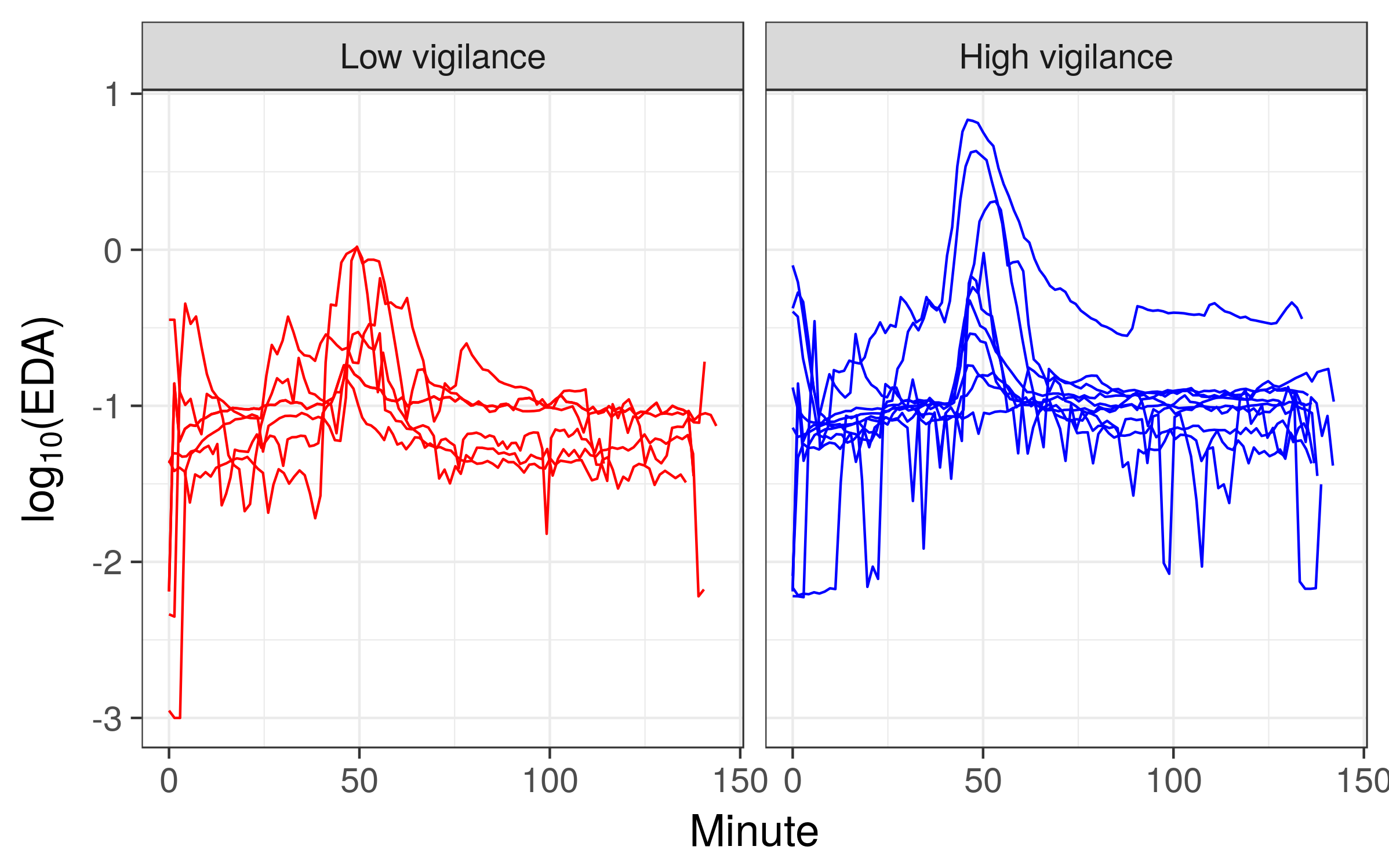
The raw EDA data are shown in Figure 10. After excluding subjects who had EDA measurements of essentially zero throughout the entire study, we were left with ten high vigilance subjects and seven low vigilance subjects.

To remove the extreme second-by-second fluctuations in EDA, which we believe are artifacts of the measurement device as opposed to real biological signals, we smoothed each curve separately with a Nadaraya–Watson kernel estimator using the ksmooth function in R. We then thinned the data to reduce computational burden, taking 100 evenly spaced measurements from each subject. Figure 11 shows the results of this process for a single subject, and Figure 12 shows the prepared data for all subjects. Because of the limited number of subjects, as well as issues of misalignment in the time series across individuals, the results presented here should be considered as illustrative rather than of full scientific validity.

9.2 Models
In all models, we fit the structure
where represents time in minutes, if subject has high vigilance and if subject has low vigilance, are random subject-specific curves, and . For , , and , we used a fourth order B-spline basis with 31 basis functions each and a second order difference penalty ().
Written in matrix notation, the penalized model is
| (34) |
where is a stacked vector for subjects , is an design matrix where and , and where is an vector of subject IDs. In other words, is equal to , but with rows corresponding to low vigilance subjects zeroed out. We set
where each is an random effects design matrix of order 4 B-splines evaluated at the input points for subject , and
where are smoothing spline penalty matrices. We also mean-centered as described in Section 3, with the corresponding changes in dimensions.
To fit a comparable penalized model, in which in (34) is replaced with , we rotated the random effect design and penalty matrices and as described in Section 3. To facilitate the use of existing software, we used a normal prior for the “unpenalized” random effect coefficients, i.e. .
We also fit a Bayesian model using the same rotations and equivalent penalties as above. In particular, we modeled the data as where
| (35) | ||||
9.3 Results
9.3.1 Frequentist estimation
We tried to use CV to estimate the smoothing parameters for the penalized model. However, with only 17 subjects split between two groups, we only did 3-fold CV. CV did not find a visually reasonable fit so we set the tuning parameters by hand.
Figure 13 shows the estimated marginal mean and 95% credible bands for the penalized model, and Figure 14 shows the subject-specific predicted curves for the penalized model. As seen in Figure 13(a), our model identified a few inflection points, particularly near minutes 40, 50, and 60. From Figure 13(b) it appears that the difference in EDA between the low and high vigilance subjects was not statistically significant. Also, as seen in Figure 14, the subject-specific predicted curves are shrunk towards the mean, which is expected, because the predicted curves are analogous to BLUPs, although they are not linear smoothers.


Figure 15 shows the estimated marginal mean and 95% credible bands for the penalized model, and Figure 16 shows the subject-specific predicted curves for the penalized model. The estimate shown in Figure 15(a) is similar to that shown in Figure 13(a), though the inflection points are slightly less pronounced in Figure 15(a). The results in Figure 15(b) are for the most part substantively the same as those in Figure 13(b); the penalized model does not show a statistically significant difference between the low and high vigilance subjects, with the possible exception of minutes 45 to 66. As seen in Figure 16, the predicted subject-specific curves from the penalized model are also shrunk towards the mean.


Table 3 shows the estimated degrees of freedom for the penalized model. Stein’s method ((19) and (20)) and the ridge approximation ((25) and (26)) were numerically instable ( and were computationally singular). Therefore we used the restricted derivative approximation to estimate the variance, as described in Section 7.1. In the penalized model, smooth had 14.2 degrees of freedom, and smooth had 6.96 degrees of freedom.
9.3.2 Bayesian estimation
We fit the model described in Section 9.2 with an element-wise Laplace prior on given by (35). To fit the model, we used rstan (Stan Development Team,, 2016) with four chains of 5,000 iterations each, with the first 2,500 iterations of each chain used as warmup. The MCMC chains, not shown, appeared to be reasonably well mixing and stationary with values under 1.1 (Gelman et al.,, 2014, see). Figure 17 shows the marginal means with 95% credible bands, and Figure 18 shows the subject-specific curves. Similar to the penalized model, the Bayesian model found a slightly statistically significant difference between low and high vigilance between minutes 42 and 65.


9.4 Alternative correlation structure
For comparison, we also fit and penalized models with alternative correlation structures similar to that recommended by Ruppert et al., (2003, p. 192).
For the penalized model, in place of the correlation structure implied by the penalty matrix described above, we set the penalty matrix to . While this is a simplification of the correlation structure recommended by Ruppert et al., (2003, p. 192), we think it offers a similar amount of flexibility.
Figure 19 shows the estimated marginal mean and 95% credible bands, and Figure 20 shows the subject-specific predicted curves. The point estimates shown in Figure 19 are similar to that shown in Figure 13. However, the confidence intervals in Figure 19 appear more reasonable. The subject-specific predicted curves shown in 20 are not shrunk towards the mean as much as in Figure 14.


For the Penalized model, in place of the correlation structure implied by the penalty matrix described above, we augmented each matrix on the left with the columns , where is an vector of measurement times for subject . We then replaced with , and assumed where
and is a common unstructured positive definite matrix. To model the within-subject correlations, we used a continuous autoregressive process of order 1. In particular, for a common parameter .
Figure 21 shows the estimated marginal mean and 95% credible bands, and Figure 16 shows the subject-specific predicted curves. The estimates shown in Figure 21 are similar to that shown in Figure 15. While estimates of the difference between low and high vigilance subjects differs between this model and the penalized model in Section 9.3, the more notable difference is in the subject-specific predicted curves. As seen in Figure 22, the predicted subject-specific curves are not shrunk towards the mean as much as in Figure 16.


Table 4 shows the mean squared error (MSE) and computing time for the penalized and penalized models. In Table 4, computing time for the penalized model does not include cross-validation, because the parameters were hand-tuned (with only 17 subjects and a complex random effects structure, cross-validation did not find reasonable parameter values). As can be seen in Table 4, the alternative correlation structure led to smaller MSE for both the and penalized models, and less computing time for the penalized model.
| penalty | penalty | |||
| Smoothing | Alternative | Smoothing | Alternative | |
| MSE | 0.0195 | 0.00649 | 0.0348 | 0.00764 |
| Computing time (seconds) | 166 | 56.9 | ||
| ∗Does not include cross-validation (parameters hand-tuned) | ||||
| Note: Models fit on a laptop with Intel i7 quad CPUs at 2.67 GHz and 8 GB memory | ||||
10 Discussion and potential extensions
As demonstrated in this article, P-splines with an penalty can be useful for analyzing repeated measures data. Compared to related work with penalties, our model is ambitious in that we allow for multiple smoothing parameters and propose approximate inferential procedures that do not require Bayesian estimation. However, these are also the two aspects of our proposed approach that require additional future work. For P-splines with an penalty, in most cases the knot placement is not critical so long as the number of knots is large enough (Ruppert,, 2002; Eilers et al.,, 2015). We believe this also holds for P-splines with an penalty, though further experimentation is needed to support this assumption. In practice, we recommend fitting models with a few different knot placements and widths to determine whether the model is sensitive to those choices for the data at hand.
Regarding estimation, our current approach of using ADMM and CV appears to work reasonably well for random intercepts, but is not yet reliable for random curves. In the future, we plan to develop more robust estimation techniques, particularly for smoothing parameters. As one possibility, we have done preliminary work to minimize quantities similar to GCV and AIC instead of the more computationally intensive CV, though these approaches do not seem as promising as their counterparts. It may also be helpful to set the degrees of freedom prior to fitting the model. When possible, Bayesian estimation may be the most reliable way to currently fit these models. Bayesian estimation also opens the possibility of using other sparsity inducing priors, such as spike and slab models (Ishwaran and Rao,, 2005).
Regarding inference, in future work it may be possible to use the quantity to bound difference between and penalized fits under certain assumptions on the data. It may also be helpful to investigate the use of post-selection inference methods to develop confidence bands for linear combinations of the active set, and to further investigate through simulations the performance of our proposed approximations of degrees of freedom. However, we note that our primary use of the degrees of freedom estimate is to obtain the residual degrees of freedom , which we then use to estimate the variances . Therefore, when , is not very sensitive to , in which case it is not critical for our purposes to obtain an exact estimate of degrees of freedom.
As for P-splines with an penalty, users must select both the order of the B-splines and the order of the finite differences. These choices will depend on the scientific problem and analytical goals. Using ( order differences) is likely an appropriate starting point for most applications, and larger could be used to increase the amount of smoothness.
For P-splines with an penalty, in most cases the knot placement is not critical so long as the number of knots is large enough (Ruppert,, 2002; Eilers et al.,, 2015). We believe this also holds for P-splines with an penalty, though further experimentation is needed to support this assumption. In practice, we recommend fitting models with a few different knot placements and widths to determine whether the model is sensitive to those choices for the data at hand.
Regarding the rate of convergence, from Observation 1 and the work of Tibshirani, 2014a (), we know that for equally spaced data and , P-splines with an penalty achieve the minimax rate of convergence for the class of weakly differentiable functions of bounded variation. When there are less knots than data points, we do not think it is possible to achieve the minimax rate of convergence. However, if the knots are selected well, it may be possible to achieve the same performance in practice.
It could also be useful to extend these results to generalized additive models to allow for non-normal responses, and to extend the approach of Sadhanala and Tibshirani, (2017) to include random effects and multiple smoothing parameters.
11 Supplementary material
We have implemented our method in the R package psplinesl1 available at https://github.com/bdsegal/psplinesl1. All code for the simulations and analyses in this paper are available at https://github.com/bdsegal/code-for-psplinesl1-paper.
Acknowlegements
We thank Margaret Hicken for sharing the data from the stress study.
Appendix A Simulated demonstration with two smooths
In this appendix, we simulated data similar to that in Section 8, but with an additional varying-coefficient smooth. In particular, we simulated data for two groups with 50 subjects in each group and between 4 and 14 measurements per subject (900 total observations). The data for subject at time was generated as where and for and . The true group means and are shown in Figure 23 and the simulated data are shown in Figure 24.


We fit a varying-coefficient model with smooths to the data. In particular, we used ADMM and 5-fold CV to minimize
| (36) |
where were formed with second order (first degree) B-splines and basis functions, where , and if observation belongs to subject and zero otherwise. We also fit an equivalent model with an penalty using the mgcv package (Wood,, 2006), i.e. with in place of in (36), .
The estimated curves are shown in Figure 25 for the penalized model and in Figure 26 for the penalized model. We used 5-fold CV to estimate the smoothing parameters and in the penalized model, and LME updates to estimate and in the final model. As seen in Figures 25 and 26, the fits are similar, but the results with the penalized model are slightly closer to the truth.


Table 5 shows the degrees of freedom and variance estimates with the penalized and penalized models. As seen in Table 5, variance estimates from both the and penalized models are very near the true values.
| Penalty | |||||
| Truth | |||||
| df (ridge) | 17.7 | 17.8 | 19.3 | 13.8 | – |
| df (Stein) | 12 | 9 | – | – | – |
| 0.0090 | 0.010 | 0.01 | |||
| 1.04 | 1.02 | 1 | |||
Appendix B Details for
Letting be the partial residuals, we can write the terms in (8) that involve as . Then taking the sub-differential of (8) with respect to , we have
| (37) |
for some where
Solving (37) for , we have . Multiplying through by and noting that is full rank and thus invertible, we have
| (38) |
Setting in (38), we get that where for all . This can only hold if , which gives us .
Appendix C Controlling total variation with the penalty
Let . Suppose the knots are equally spaced, and let for all and . Then on the interval , from (De Boor,, 2001, p. 117) we have
| (39) |
where is the order backwards difference.
Let . We note that is finite and positive for all . Then from (39), we have
| (40) | ||||
| (41) |
where (40) follows because .
Rewriting (41), for we have
where is a constant. This shows that controlling the norm of the order finite differences in coefficients also controls the total variation of the derivative of the function.
References
- Bollaerts et al., (2006) Bollaerts, K., Eilers, P. H. C., and Aerts, M. (2006). Quantile regression with monotonicity restrictions using P-splines and the L1-norm. Statistical Modelling, 6(3):189–207.
- Boyd et al., (2011) Boyd, S., Parikh, N., Chu, E., Peleato, B., and Eckstein, J. (2011). Distributed optimization and statistical learning via the alternating direction method of multipliers. Foundations and Trends® in Machine Learning, 3(1):1–122.
- Chen and Wang, (2011) Chen, H. and Wang, Y. (2011). A penalized spline approach to functional mixed effects model analysis. Biometrics, 67(3):861–870.
- De Boor, (2001) De Boor, C. (2001). A practical guide to splines. Springer, New York, NY, revised edition.
- Donoho and Johnstone, (1988) Donoho, D. L. and Johnstone, I. M. (1988). Minimax estimation via wavelet shrinkage. The Annals of Statistics, 26(3):879 – 921.
- Efron, (1986) Efron, B. (1986). How biased is the apparent error rate of a prediction rule. Journal of the American Statistical Association, 81(394):461–470.
- Eilers, (2000) Eilers, P. H. C. (2000). Robust and quantile smoothing with P-splines and the L1 norm. In Proceedings of the 15th International Workshop on Statistical Modelling, Bilbao.
- Eilers and Marx, (1996) Eilers, P. H. C. and Marx, B. D. (1996). Flexible smoothing with B-splines and penalties. Statistical science, 11(2):89–121.
- Eilers et al., (2015) Eilers, P. H. C., Marx, B. D., and Durbán, M. (2015). Twenty years of p-splines. SORT: statistics and operations research transactions, 39(2):149–186.
- Fitzmaurice et al., (2008) Fitzmaurice, G., Davidian, M., Verbeke, G., and Molenberghs, G. (2008). Longitudinal data analysis. Chapman and Hall/CRC, Boca Raton, FL.
- Gelman et al., (2014) Gelman, A., Carlin, J. B., Stern, H. S., Dunson, D. B., Vehtari, A., and Rubin, D. B. (2014). Bayesian data analysis. Chapman and Hall/CRC, Boca Raton, FL, 3rd edition.
- Gelman et al., (2008) Gelman, A., Jakulin, A., Pittau, M. G., and Su, Y.-S. (2008). A weakly informative default prior distribution for logistic and other regression models. The Annals of Applied Statistics, 2(4):1360–1383.
- Green, (1987) Green, P. J. (1987). Penalized likelihood for general semi-parametric regression models. International Statistical Review, 55(3):245 – 259.
- Guo, (2002) Guo, W. (2002). Functional mixed effects models. Biometrics, 58(1):121–128.
- Hastie and Tibshirani, (1986) Hastie, T. and Tibshirani, R. (1986). Generalized additive models. Statistical Science, 1:297–318.
- Hastie and Tibshirani, (1990) Hastie, T. and Tibshirani, R. (1990). Generalized Additive Models. Monographs on Statistics and Applied Probability. Chapman & Hall, London, 1st edition.
- Hastie and Tibshirani, (1993) Hastie, T. and Tibshirani, R. (1993). Varying-coefficient models. Journal of the Royal Statistical Society: Series B (Statistical Methodology), 55(4):757–796.
- Ishwaran and Rao, (2005) Ishwaran, H. and Rao, J. S. (2005). Spike and slab variable selection: Frequentist and bayesian strategies. The Annals of Statistics, 33(2):730 – 773.
- Janson et al., (2015) Janson, L., Fithian, W., and Hastie, T. J. (2015). Effective degrees of freedom: a flawed metaphor. Biometrika, pages 1–8.
- Kim et al., (2009) Kim, S.-J., Koh, K., Boyd, S., and Gorinevsky, D. (2009). trend filtering. SIAM review, 51(2):339–360.
- Lin et al., (2006) Lin, Y., Zhang, H. H., et al. (2006). Component selection and smoothing in multivariate nonparametric regression. The Annals of Statistics, 34(5):2272–2297.
- Lou et al., (2016) Lou, Y., Bien, J., Caruana, R., and Gehrke, J. (2016). Sparse partially linear additive models. Journal of Computational and Graphical Statistics, 25(4).
- Mammen et al., (1997) Mammen, E., van de Geer, S., et al. (1997). Locally adaptive regression splines. The Annals of Statistics, 25(1):387–413.
- Meier et al., (2009) Meier, L., Van de Geer, S., and Bühlmann, P. (2009). High-dimensional additive modeling. The Annals of Statistics, 37(6B):3779–3821.
- Petersen et al., (2016) Petersen, A., Witten, D., and Simon, N. (2016). Fused lasso additive model. Journal of Computational and Graphical Statistics, 25(4):1005–1025.
- R Core Team, (2017) R Core Team (2017). R: A Language and Environment for Statistical Computing. R Foundation for Statistical Computing, Vienna, Austria.
- Ramdas and Tibshirani, (2016) Ramdas, A. and Tibshirani, R. J. (2016). Fast and flexible ADMM algorithms for trend filtering. Journal of Computational and Graphical Statistics, 25(3):839–858.
- Ravikumar et al., (2009) Ravikumar, P., Lafferty, J. D., Liu, H., and Wasserman, L. (2009). Sparse additive models. Journal of the Royal Statistical Society: Series B (Statistical Methodology), 71(5).
- Rice and Wu, (2001) Rice, J. A. and Wu, C. O. (2001). Nonparametric mixed effects models for unequally sampled noisy curves. Biometrics, 57(1):253–259.
- Ruppert, (2002) Ruppert, D. (2002). Selecting the number of knots for penalized splines. Journal of computational and graphical statistics, 11(4):735–757.
- Ruppert et al., (2003) Ruppert, D., Wand, M. P., and Carroll, R. J. (2003). Semiparametric regression. Cambridge University Press, New York, NY.
- Sadhanala and Tibshirani, (2017) Sadhanala, V. and Tibshirani, R. J. (2017). Additive models with trend filtering. arXiv preprint arXiv:1702.05037.
- Scheipl et al., (2015) Scheipl, F., Staicu, A.-M., and Greven, S. (2015). Functional additive mixed models. Journal of Computational and Graphical Statistics, 24(2):447–501.
- Speed, (1991) Speed, T. (1991). Comment on “That BLUP is a good thing: The estimation of random effects”. Statistical science, 6(1):42–44.
- Stan Development Team, (2016) Stan Development Team (2016). RStan: the R interface to Stan. R package version 2.14.1.
- Stein, (1981) Stein, C. M. (1981). Estimation of the mean of a multivariate normal distribution. The Annals of Statistics, 9(6):1135 – 1151.
- Tibshirani, (1996) Tibshirani, R. (1996). Regression shrinkage and selection via the lasso. Journal of the Royal Statistical Society: Series B (Methodological), 58(1):267 – 288.
- Tibshirani et al., (2005) Tibshirani, R., Saunders, M., Rosset, S., Zhu, J., and Knight, K. (2005). Sparsity and smoothness via the fused lasso. Journal of the Royal Statistical Society: Series B (Statistical Methodology), 67(1):91–108.
- (39) Tibshirani, R. J. (2014a). Adaptive piecewise polynomial estimation via trend filtering. The Annals of Statistics, 42(1):285–323.
- (40) Tibshirani, R. J. (2014b). Supplement to “adaptive piecewise polynomial estimation via trend filtering”.
- Tibshirani and Taylor, (2012) Tibshirani, R. J. and Taylor, J. (2012). Degrees of freedom in lasso problems. The Annals of Statistics, (2):1198–1232.
- Wahba, (1990) Wahba, G. (1990). Spline models for observational data. Society for industrial and applied mathematics, Philadelphia, PA.
- Wang, (1998) Wang, Y. (1998). Mixed effects smoothing spline analysis of variance. Journal of the Royal Statistical Society: Series B (Statistical Methodology), 60(1):159–174.
- Wang et al., (2014) Wang, Y.-X., Smola, A., and Tibshirani, R. (2014). The falling factorial basis and its statistical applications. In International Conference on Machine Learning, pages 730–738.
- Wood, (2004) Wood, S. N. (2004). Stable and efficient multiple smoothing parameter estimation for generalized additive models. Journal of the American Statistical Association, 99(467):673–686.
- Wood, (2006) Wood, S. N. (2006). Generalized additive models: an introduction with R. Chapman and Hall/CRC, Boca Raton, FL.
- Wood, (2011) Wood, S. N. (2011). Fast stable restricted maximum likelihood and marginal likelihood estimation of semiparametric generalized linear models. Journal of the Royal Statistical Society: Series B (Statistical Methodology), 73(1):3–36.
- Wood et al., (2015) Wood, S. N., Goude, Y., and Shaw, S. (2015). Generalized additive models for large data sets. Journal of the Royal Statistical Society: Series C (Applied Statistics), 64(1):139–155.
- Wood et al., (2016) Wood, S. N., Pya, N., and Säfken, B. (2016). Smoothing parameter and model selection for general smooth models. Journal of the American Statistical Association, 111(516):1548 – 1575.
- Yuan and Lin, (2006) Yuan, M. and Lin, Y. (2006). Model selection and estimation in regression with grouped variables. Journal of the Royal Statistical Society: Series B (Statistical Methodology), 68(1):49 – 67.
- Zhang et al., (1998) Zhang, D., Lin, X., Raz, J., and Sowers, M. (1998). Semiparametric stochastic mixed models for longitudinal data. Journal of the American Statistical Association, 93(442):710 – 719.
- Zhao et al., (2009) Zhao, P., Rocha, G., and Yu, B. (2009). The composite absolute penalties family for grouped and hierarchical variable selection. The Annals of Statistics, 37(6A):3468 – 3497.
- Zou and Hastie, (2005) Zou, H. and Hastie, T. (2005). Regularization and variable selection via the elastic net. Journal of the Royal Statistical Society: Series B (Statistical Methodology), 67(2):301 – 320.