Analog On-Tag Hashing: Towards Selective Reading as Hash Primitives in Gen2 RFID Systems
Abstract.
Deployment of billions of Commercial off-the-shelf (COTS) RFID tags has drawn much of the attention of the research community because of the performance gaps of current systems. In particular, hash-enabled protocol (HEP) is one of the most thoroughly studied topics in the past decade. HEPs are designed for a wide spectrum of notable applications (e.g., missing detection) without need to collect all tags. HEPs assume that each tag contains a hash function, such that a tag can select a random but predicable time slot to reply with a one-bit presence signal that shows its existence. However, the hash function has never been implemented in COTS tags in reality, which makes HEPs a 10-year untouchable mirage. This work designs and implements a group of analog on-tag hash primitives (called Tash) for COTS Gen2-compatible RFID systems, which moves prior HEPs forward from theory to practice. In particular, we design three types of hash primitives, namely, tash function, tash table function and tash operator. All of these hash primitives are implemented through selective reading, which is a fundamental and mandatory functionality specified in Gen2 protocol, without any hardware modification and fabrication. We further apply our hash primitives in two typical HEP applications (i.e., cardinality estimation and missing detection) to show the feasibility and effectiveness of Tash. Results from our prototype, which is composed of one ImpinJ reader and Alien tags, demonstrate that the new design lowers of the communication overhead in the air. The tash operator can additionally introduce an overhead drop of .
Keywords:
RFID; Hash Function; Hash Table Function; EPCGlobal Gen21. Introduction
RFID systems are increasingly used in everyday scenarios, which range from object tracking, indoor localization (Yang et al., 2014), vibration sensing (Yang et al., 2016), to medical-patient management, because of the extremely low cost of commercial RFID tags (e.g., as low as 5 cents per tag). Recent reports show that many industries like healthcare and retailing are moving towards deploying RFID systems for object tracking, asset monitoring, and emerging Internet of Things (Frost and Sullivan, 2011).
1.1. The State-of-the-Art
The Electronic Product Code global is an organization established to accomplish the worldwide adoption and standardization of EPC technology. It published the Gen2 air protocol (gen, 2004) for RFID system in 2004. A Gen2 RFID system consists of a reader and many passive tags. The passive tags without batteries are powered up purely by harvesting radio signals from readers. This protocol has become the mainstream specification globally, and has been adopted as a major part of the ISO/IEC 18000-6 standard.
Embedding Gen2 tags into everyday objects to construct ubiquitous networks has been a long-standing vision. However, a major problem that challenges this vision is that the Gen2 RFID system is not efficient (Wang et al., 2012). First, the RFID system utilizes simple modulations (e.g., ON-OFF keying or BPSK) due to the lack of traditional transceiver (Dobkin, 2012), which prevents tags from leveraging a suitable channel to transmit more bits per symbol and increase the bandwidth efficiency. Second, tags cannot hear the transmissions of other tags. They merely reply on the reader to schedule their medium access with the Framed Slotted ALOHA protocol, which results in many empty and collided slots. This condition also retards the inventory process. These two limitations force a reader to go through a long inventory phase when it collects all the tags in the scene.
1.2. Ten-Year Mirage of HEP
Motivated by the aforementioned performance gaps, the research community opened a new focus on HEP design approximately 10 years ago. The key idea that underlies HEPs is that each tag selects a time slot according to the hash value of its EPC and a random seed. It then replies a one-bit presence signal rather than the entire EPC number in the selected slot. HEPs treat all tags as if they were a virtual sender, which outputs a gimped hash table (i.e., a presence bitmap) when responding to a challenge (i.e., a random seed). Most importantly, HEPs assume the backend server and every tag share a hash function, and the resulting bitmap is random but predicable when the EPCs and seeds are known.
Fig. 1 shows a toy example with tags, each of which contains a unique EPC number presented in binary format (e.g., ), to illustrate the HEP concept. The reader divides the time into time slots (e.g., .) and challenges these tags with the random seed . Each tag selects the time slot to reply the one-bit signal, where is a common hash function (e.g., MD5, SHA-1) and . The reader can recognize two possible results for each time slot, namely, empty and non-empty11 1 Some work assume the reader can recognize the signal collision, obtaining three results: empty, single and collision. . The reader abstracts the reply results into a bitmap (i.e., ), where each element contains two possible values, that is, and , that corresponds to empty and non-empty slots, respectively. The upper layer then utilizes this returned bitmap to explore many notable applications. We show the following two typical applications as examples to drive the key point:
Cardinality estimation. Estimating the size of a given tag population is required in many applications, such as privacy sensitive systems and warehouse monitoring. Kodialam et al. (Kodialam and Nandagopal, 2006) presented a pioneer estimator. Given that tags select the time slots uniformly because of hashing, the expected number of ‘’s equals . Counting in an instance yields a “zero estimator”, i.e., . For example, in our toy example.
Missing detection. Consider a major warehouse that stores thousands of apparel, shoes, pallets, and cases. How can a staff immediately determine if anything is missing? Sheng and Li (Tan et al., 2008) conducted the early study on the fast detection of missing-tag events by using the presence bitmap. They assumed all EPCs were known in a closed system. Given that hash results are predicable, the system can generate an intact bitmap at the backend. We can identify the missing tags in a probabilistic approach by comparing the intact and instanced bitmaps. For example, if the second entry equals (which is supposed to be ), the the tag must be missing in our toy example.
HEPs are advantageous in terms of speed and privacy. HEPs are faster than all prior per-tag reading schemes for two reasons. First, collecting all the EPCs of the tags is time consuming because of the aforementioned low-rate modulation, whereas one-bit presence signals of HEPs save approximately of the time (i.e., the EPC length equals 96 bits in theory 22 2 Actual case in practice would be less than this estimate due to other extra jobs, such as setup time, query time, etc.). Second, collisions are considered as one of the major reasons that drag down the reading. On the contrary, HEPs tolerate and consider collisions as informative. When privacy issues are considered, the tag’s identification may be unacceptable in certain instances. HEPs allow tags to send out non-identifiable information (i.e., one-bit signals).
HEPs are very promising. However, after 10 years of enthusiastic discussion about the opportunities that HEPs provide, the reality is beginning to settle: the functionality of hashing (i.e., hash function and hash table function) has never been implemented in any Gen2 RFID tags and considered by any RFID standard. No hint shows that this function will be widely accepted in the near future.
1.3. Why Not Support Hashing?
A large number of recent work have attempted to supplement hash functionality to RFID tags, which can be categorized into three groups. First group, like (Feldhofer and Rechberger, 2006; Poschmann et al., 2007), modifies the common hash functions to accommodate resource-constrained RFID tags. The second group (Yoshida et al., 2007; Bogdanov et al., 2007; Rolfes et al., 2008; Bogdanov et al., 2007; Poschmann et al., 2007; Lim and Korkishko, 2005; Yu et al., [n. d.]; Hong et al., 2006; Good and Benaissa, 2007) designs new lightweight and efficient hash functions dedicatedly for RFID tags. The third group seeks new design of RFID tags like WISP(Philipose et al., 2005) and Moo (Zhang et al., 2011a), which gives tags more powerful computing capabilities (e.g., hashing (Pendl et al., 2012)). Unfortunately, as far as we know, none of these work has been really applied in COTS RFID systems yet.
Why is the hash function unfavored? A term called as Gate Equivalent (GE) is widely used to evaluate a hardware design with respect to its efficiency and availability. One GE is esquivalient to the area which is required by the two-input NAND gate with the lowest deriving strength of the corresponding technology. A glance at Table. 5 shows the available designs of hash functions for RFID tags require a significant number of GEs, which are completely unaffordable by current COTS tags. For example, the most compact hash functions requires thousands of GEs (e.g., GEs for PRESENT-80), which incur extremely high energy consumption and manufacture cost. Thus, relatively few RFID-oriented protocols that appeal to a hash function can be utilized. RFID was expected to be one of the most competitive automatic identification technologies due to its many attractive advantages (e.g., simultaneous reading, NLOS, etc.) compared with others (e.g., barcode). However, this progress has been hindered for many years by the final obstacle that the industry is attempting to overcome (i.e., the price). The industry is extremely sensitive to the cost being doubled or tripled by the hash, although HEPs actually introduce significant outperformance.
1.4. Our Contributions
This work designs a group of hash primitives, Tash, which takes advantage of existing fundamental function of selective reading specified in Gen2 protocol, without any hardware modification and fabrication. Our design and implementation both strictly follow the Gen2 specification, so it can work in any Gen2-Compatible RFID system. These mimic (or analog) hash primitives act as we embedded real hash circuits on tags33 3 This work does not target at designing any analog circuit on readers or tags, but offers a mimic hash function acting as we embed a hash circuit on each tag., while we actually implement them in application layer. Specifically, we design the following three kinds of hash primitives to revive prior HEPs:
We design a hash function (aka tash function) over existing COTS Gen2 tags. The hash function outputs a hash value associated with the EPC of the tag and a random seed, as HEPs require.
We design a hash table function (aka tash table function) over all tags in the scene. It can produce a hash table (aka tash table), which is more informative than a bitmap, over the all tags in the scene. In particular, each entry indicates the exact number of tags hashed into this entry.
Major prior HEPs require multiple acquisitions of bitmaps to meet an acceptable confidence. We design three tash operators (i.e., tash AND, OR and XOR) to perform entry-wise set operations over multiple tash tables on tag in the physical layer, which offers a one-stop acquisition solution.
Summary. It has been considered that HEPs are hardly applied in practice because of the ‘impossible mission’ of implementing hash function on COTS Gen2 tags (Bogdanov et al., 2008). In this work, our main contribution lies in the practicality and usability, that is, enabling billions of deployed tags to benefit performance boost from prior well-studied HEPs, with our hash primitives. To the best of our knowledge, this is the first work to implement the hash functionality over COTS Gen2 tags. Second, we provide an implementation of Tash and show its feasibility and efficiency in two typical usage scenarios. Third, we investigate several leading RFID products in market including types of tags and types of readers, in terms of their compatibility with Gen2, and conduct an extensive evaluation on our prototype with COTS devices.
2. Related Work
We review the related work from two aspects: the designs of hash functions and hash enabled protocols.
Design of hash function. Feldhofer and Rechberger (Feldhofer and Rechberger, 2006) firstly point that current common hash functions (e.g., MD5, SHA-1, etc.), are not hardware friendly and unsuitable at all for RFID tags, which have very constrained computing ability. Such difficulty has spurred considerable research (Feldhofer and Rechberger, 2006; Yoshida et al., 2007; Bogdanov et al., 2007; Rolfes et al., 2008; Bogdanov et al., 2007; Poschmann et al., 2007; Lim and Korkishko, 2005; Yu et al., [n. d.]; Hong et al., 2006; Poschmann et al., 2007; Good and Benaissa, 2007). We sketch the primary designs and their features in Table. 5. For example, Bogdanov et al. (Bogdanov et al., 2007) propose a hardware-optimized block cipher, PRESENT, designed with area and power constraints. The follow-up work (Rolfes et al., 2008) presents three different architectures of PRESENT and highlights their availability for both active and passive smart devices. Their implementations reduce the number of GEs to around. Another follow-up work (Bogdanov et al., 2008) extends the design of PRESENT and gives 8 variants to fulfill different requirements, e.g., DM-PRESENT-80, DM-PRESENT-128, H-PRESENT-128, etc. The work (Poschmann et al., 2007) suggests to choose DES as hash function for RFID tags due to relatively low complexity, and presents a variant of DES, called asi.e., DESXL. Lim and Korkishko (Lim and Korkishko, 2005) present a -bit hash function with three key size options ( bits, bits and bits), which requires about and GEs. In summary, despite these optimized designs, majority are still presented in theory and none of them are available for the COTS RFID tags. On contrary, our work explores hash function from another different aspect, that is, leveraging selective reading to mimic equivalent hash primitives.
| Hash functions | Key size | GE | Power | Clock cycles |
|---|---|---|---|---|
| SHA-256(Feldhofer and Rechberger, 2006) | 256 | 10,868 | 15.87 | 1,128 |
| SHA-1 (Feldhofer and Rechberger, 2006) | 160 | 8,120 | 10.68 | 1,274 |
| AES (Feldhofer et al., 2004) | 128 | 3,400 | 8.15 | 1,032 |
| MAME(Yoshida et al., 2007) | 256 | 8,100 | 5.16 | 96 |
| MD5 (Feldhofer and Rechberger, 2006) | 128 | 8,400 | - | 612 |
| MD4 (Feldhofer and Rechberger, 2006) | 128 | 7,350 | - | 456 |
| PRESENT-80 (Bogdanov et al., 2007) | 80 | 1,570 | - | 32 |
| PRESENT-80 (Rolfes et al., 2008) | 80 | 1,075 | - | 563 |
| PRESENT-128 (Bogdanov et al., 2008) | 128 | 1,886 | - | 32 |
| DES (Poschmann et al., 2007) | 56 | 2,309 | - | 144 |
| mCrypton (Lim and Korkishko, 2005) | 96 | 2,608 | - | 13 |
| TEA (Yu et al., [n. d.]) | 128 | 2,355 | - | 64 |
| HIGHT (Hong et al., 2006) | 128 | 3,048 | - | 34 |
| DESXL (Poschmann et al., 2007) | 184 | 2,168 | - | 144 |
| Grain & Trivium(Good and Benaissa, 2007) | 80 | 2,599 | - | 1 |
Design of hash enabled protocol. To drive our key point, we conduct a brief survey of previous related works. We list several key usage scenarios that we would like to support. Our objective is not to complete the list, but to motivate our design. (1) Cardinality estimation. Dozens of estimators (Kodialam et al., 2007; Sheng et al., 2008; Sze et al., 2009; Qian et al., 2010; Qian et al., 2011; Shah-Mansouri and Wong, 2011; Shahzad and Liu, 2012; Zheng and Li, 2013b; Chen et al., 2013; Xiao et al., 2013; Gong et al., 2014; Liu et al., 2014c; Zheng and Li, 2014; Liu et al., 2015b; Hou et al., 2015) have been proposed in the past decade. For example, Qian et al. (Qian et al., 2011) proposed an estimation scheme called lottery frame. Shahzad and Liu (Shahzad and Liu, 2012) estimated the number based on the average run-length of ones in a bit string received using the FSA. In particular, they claimed that their protocol is compatible with Gen2 systems. However, their scheme still requires modifying the communication protocol, and thus, it fails to work with COTS Gen2 systems. By contrast, our prototype can operate in COTS Gen2 systems as demonstrated in this study. (2) Missing detection. The missing detection problem was firstly mentioned in (Tan et al., 2008). Thereafter, many follow-up works (Li et al., 2010a; Luo et al., 2011; Zhang et al., 2011b; Luo et al., 2012; Zheng and Li, 2015; Tan et al., 2010; Li et al., 2013; Liu et al., 2014b; Luo et al., 2014; Ma et al., 2012; Xie et al., 2014b; Shahzad and Liu, 2015; Shahzad and Liu, 2016; Yu et al., 2016; Yu et al., 2015) have started to study the issue of false positives resulting from the collided slots by using multiple bitmaps. Additional details regarding this application are introduced in 5. (3) Continuous reading. The traditional inventory approach starts from the beginning each time it interrogates all the tags, thereby making it highly time-inefficient. These works (Sheng et al., 2010; Xie et al., 2013; Liu et al., 2014a) have proposed continuous reading protocols that can incrementally collect tags in each step using the bitmap. For example, Sheng et al. (Sheng et al., 2010) aimed to preserve the tags collected in the previous round and collect only unknown tags. Xie et al. (Xie et al., 2013) conducted an experimental study on mobile reader scanning. Liu et al. (Liu et al., 2014a) initially estimated the number of overlapping tags in two adjacent inventories and then performed an effective incremental inventory. (4) Data mining. These works (Sheng et al., 2008; Xie et al., 2014a; Luo et al., 2013; Luo et al., 2016; Liu et al., 2015a) discuss how to discover potential information online through bitmaps. For example, Sheng et al. (Sheng et al., 2008) proposed to identify the popular RFID categories using the group testing technique. Xie et al. found histograms over tags through a small number of bitmaps(Xie et al., 2014a). Luo et al. (Luo et al., 2013; Luo et al., 2016) determined whether the number of objects in each group was above or below a threshold. Liu et al. (Liu et al., 2015a) proposed a new online classification protocol for a large number of groups. (5) Tag searching. These works(Liu et al., 2015c; Zheng and Li, 2013a) have studied the tag searching problem that aims to find wanted tags from a large number of tags using bitmaps in a multiple-reader environment. Zheng et al. (Zheng and Li, 2013a) utilized bitmaps to aggregate a large volume of RFID tag information and to search the tags quickly. Liu et al. (Liu et al., 2015c) first used the testing slot technique to obtain the local search result by iteratively eliminating wanted tags that were absent from the interrogation region. (6) Tag polling. (Qiao et al., 2011; Qiao et al., 2013; Li et al., 2016) consider how to quickly obtain the sensing information from sensor-augmented tags. The system requires to assign a time slot to each tag using the presence bitmap. In summary, all the aforementioned HEP designs have allowed RFID research to develop considerably in the past decade. All the work can be boosted by our hash primitives.
3. Overview
Tash is a software framework that provides a group of fundamental hash primitives for HEPs. This section presents its usage scope and formally defines our problem domain.
3.1. Scope
Despite clear and certain specifications, the implementation of the Gen2 protocol still varies with readers and manufacturers because of firmware bugs or compromises, especially in early released reader devices, according to our compatibility report presented in 7. Here, we firmly claim that our design and implementation strictly follow the specifications of the Gen2 and LLRP protocols (refer to 6). The framework works with any Gen2-compatible readers and tags. The performance losses caused by defects in devices are outside the scope of our discussion.
3.2. Definitions of Hash Primitives
Before delving into details, we formally define the hash primitives that the HEPs require, from a high-level.
Definition 1 (Tash function).
An -bit tash function is actually a hash function , where and are the domains of EPCs of the tags and random seeds.
Tash function and tash value. As the above definition specifies, an -bit tash function takes an EPC and a random seed as input and outputs an -bit integer , denoted by:
| (1) |
We call the dimension of tash function (i.e., ). The tash value is an integer . Similar to other common hash function, the tash function has three basic characteristics. First, the output changes significantly when the two parameters are altered. Second, its output is uniformly distributed within the given range, and predicable if all inputs are known. Third, the hash values are accessible.
Definition 2 (Tash table function).
An -bit tash table function can assign each tag from a given set into the entry of a hash table (aka tash table) with a random seed , where . Each entry of the tash table is the number of tags tashed into it.
Tash table function and tash table. Let and denote a tash table and a tash table function respectively. The tash table function takes a set of tags (i.e., ) and a random number as input and outputs a tash table , denote by:
| (2) |
where (i.e., the number of tags tashed into the entry) for . Let , which is defined as the size of the tash table. The tash table function is the core function that HEPs expect. HEPs consider the reader as well as all tags as a black box equipping with tash table function. When inputing a random seed, the box would output a tash table. HEPs then utilize such table to provide various services (e.g., missing detection or cardinality estimation.). It worths noting that superior to the bitmap employed in prior HEPs, our tash table is a perfect table that contains the exact number of tags tashed into each entry. Clearly, the table is completely backward compatible with prior HEPs because it can be forcedly converted into a presence bitmap.
Tash operators. Most prior HEPs adopt probabilistic ways and their results are guaranteed with a given confidence level. To meet the level, they usually combine multiple bitmaps, which are acquired through multiple rounds and challenged by different seeds. We abstract such combination into three basic tash operators, namely, tash AND, OR and XOR. These operators can comprise other complex operations. Let and denote two tash tables acquired twice with two different seeds, and .
Definition 3 (Tash AND).
The tash AND (denoted by ) of two tash tables is to obtain the intersection of two corresponding entry sets. Formally, , where .
The tash AND is aimed at obtaining the common intersection of corresponding entries from two tash tables. For example, as shown in Fig. 2, and count and respectively. However, , which counts only.
Definition 4 (Tash OR).
The tash OR (denoted by ) of two tash tables is to merge two corresponding entry sets. Formally, , where .
The tash OR is aimed at obtaining the total number of tags mapped into the corresponding entries in two tash tables. Note tash OR is not the same as the entry-wise sum, i.e., because the tags twice mapped into a same entry are counted only once. As shown in Fig. 2, although because and appear twice in the two tash tables.
Definition 5 (Tash XOR).
The tash XOR (denoted by ) is to remove the intersection of two corresponding entry sets from the first entry set. Formally, such that .
The tash XOR is aimed at obtaining the total number of the set difference. As Fig. 2 shows, and . Then .
The above operators can be applied in a series of tash tables with the same dimension for a hybrid operation, e.g., . Tash AND and OR satisfy operational laws such as associative law and commutative law, e.g., . The design of tash operators is one of the attractive features of the tash framework, and it has never been proposed before. More importantly, we design and implement these operators in the physical layer to provide one-stop acquisition solution.
3.3. Solution Sketch
Tash is designed to reduce the overhead for air communications. It runs in the middle of the reader and upper application. The upper application passes a pair of arguments (i.e., and ), or pairs of arguments (as well as operators) to Tash. On the basis of the arguments, Tash generates one or more configuration files to manipulate the reader’s reading. Finally, Tash abstracts the reading results to a tash table, which is returned to the upper application.
The rest of the paper is structured as follows. We firstly present the tash design in 4. We next demonstrate the usage of our hash primitives in two classic applications in 5. We then introduce the tash implementation using LLRP interfaces in 6. In 7 and 8, we present the microbenchmark and the usage evaluation. Finally, we conclude in 9 and present future directions.
4. Tash Design
In this section, we introduce the background of selective reading in Gen2, and then present the technical details of our designs.
4.1. Background of Gen2 Protocol
The Gen2 standard defines air communication between readers and tags. On the basis of (gen, 2004; Zhang et al., 2009), we introduce its four central functions we will employ:
F1: Memory Model. Gen2 specifies a simple tag memory model (pages 44 46 of (gen, 2004)). Each tag contains four types of non-volatile memory blocks (called memory banks): (1) MemBank-0 is reserved for password associated with the tag. (2) MemBank-1 stores the EPC number. (3) MemBank-2 stores the TID that specifies the unchangeable tag and vendor specific information. (4) MemBank-3 is a customized storage that contains user-defined data.
F2: Selective Reading. Gen2 specifies that each inventory must be started with Select command (pages 7273 of (gen, 2004)). The reader can use this command to choose a subset of tags that will participate in the upcoming inventory round. In particular, each tag maintains a flag variable SL. The reader can use the Select command to turn the SL flags of tags into asserted (i.e., true) or deasserted (i.e., false). The Select command comprises six mandatory fields and one optional field apart from the constant cmd code (i.e., ), as shown in Fig. 3. The following fields are presented for this study.
| Action code | Tag matching | Tag not-matching |
|---|---|---|
| assert SL | deassert SL | |
| assert SL | do nothing | |
| do nothing | deassertSL | |
| negate SL | do nothing | |
| deassert SL | assert SL | |
| deassert SL | do nothing | |
| do nothing | assert SL | |
| do nothing | negate SL |
Target. This field allows a reader to change SL flags or the inventoried flags of the tags. The inventoried flags are used when multiple readers are present. Such scenario is irrelevant to our requirements. Thus, we aim to change SL flags only by setting Target=.
Action. This field specifies an action that will be will performed by the tags. Table. 2 lists eight action codes to which the tag makes different responses. For example, the matching or not-matching tags assert or deassert their SL flags when Action=. We leverage this useful feature to design tash operators.
MemBank, Pointer, Length and Mask. These four fields are combined to compose a bitmask. The bitmask indicates which tags are matched or not-matched for an Action. The Mask contains a variable length binary string that should match the content of a specific position in the memory of a tag. The Length field defines the length of the Mask field in bits. The Mask field can be compared with one of the four types of memory banks in a tag. The MemBank field specifies which memory bank the Mask will be compared with. The Pointer field specifies the starting position in the memory bank where the Mask will be compared with. For example, if we use a tuple to denote the four fields, then only the tags with data starting at the bit with a length of bits in the memory bank that is equal to are matched.
To visually understand the selective reading, we show an example in Fig. 4 in which 4 out of 7 tags are selected to participate in the incoming inventory. Complex and multiple subsets of tags can be facilitated by issuing a group of Select commands to choose a subset of tags before an inventory round starts. For example, we can issue two Select commands: one for division and another for one-bit reply. Note the Truncate enabled Select command must be the last one if multiple selection commands are issued (gen, 2004).
F3: Truncated Reply. Gen2 allows tags to reply a truncated reply (i.e., replying a part of EPC) through a special Select command with an enabled Truncate field, making a one-bit presence signal possible. When Truncate is enabled (i.e., set to ), then the corresponding bitmask is not used for the division of tags, but lets tags reply with a portion of their EPCs following the pattern specified by the bitmask. Note that when Truncate is enabled, the MemBank must be set to the EPC bank (i.e., ) and such Select command must be the last one.
F4: Query Model. Followed by a group of Select commands, Query command (see page 7680 of (gen, 2004).) starts a new inventory round over a subset of tags, chosen by the previous Select commands. There are fields in the Query command. We only focus on Sel field, which is most tightly relevant to the selective reading. As mentioned above, the Select command has divided the tags into two opposite subsets with asserted and deasserted SL respectively. The Sel field specifies which subset will reply in the current inventory round. If Sel=, the tags with asserted SL reply. If Sel=, the tags with deasserted SL reply. We choose the tags with asserted SL by default.
4.2. Design of the Tash Function
An -bit tash function is essentially a hash function that is indispensable to HEPs. We design the tash function while following the three principles outlined as follows. The first principle requires that the tash result must be dependent on the input EPC and the seed. Moreover, it must be predictable as long as all the input parameters are known. The second principle requires the output values to be random, i.e., uniformly distributed in . Even a one bit difference in the input will result in a completely different outcome. The third principle requires a method that can access the tash result of a tag directly or indirectly.
We have constructed the tash function as follows by applying the aforementioned principles: given a tag with an EPC of , we firstly calculate the hash value of the EPC offline, using a common perfect hash function like -bit MD5 or SHA-1. Let denote the calculated hash value. We then write into the tag’s user-defined memory bank of the tag, i.e., MemBank-3, for later use.
Definition 6 (Tash value).
The -bit tash value of tag challenged by seed is defined as the value of the sub-bitstring starting from the bit and ending at the bit in the MemBank-3 of the tag.
Evidently, is actually a portion of , and thus, the parameter and , where is the length of the hash value (e.g., bits). Fig. 5 shows an example wherein the MemBank-1 and MemBank-3 of the tag store its EPC and the hash value , respectively. When and are inputted, the tash value that this tag outputs is , which is the sub-bitstring of starting from the bit and ending at the bit in MemBank-3, i.e., .
Our design does not require a tag to equip a real hash function or the engagement of its chip. It clearly applies the preceding principles. First, is evidently repeatable, predicable and dependent on the inputs. Second, the randomness of is derived from and , which are supposed to have a good randomness quality. Third, we have two ways to access the tash value. We can use the memory Read command to access MemBank-3 of a tag directly, or use the selective reading function to access the tash value indirectly (discussed later).
Discussion: A few points are worth-noting about the design:
As the tash value is a portion of the hash value, if two random numbers may cover a common sub-string. For example, if and differ by , there exist same bits with of probability that two hash values are same, although such case occurs with a small probability, i.e., . If some upper applications require extremely strong independence, we should generate the second random number meeting the condition of and , so as to avoid the common coverage and potential relevance.
The design of tash function involves the MemBank-3, i.e., the user-defined storage. We can use Write command to store any data into this memory bank. Our compatibility report (shown in 7) suggests that almost all types of tags support both MemBank-3 and Write command except one read-only type (i.e., ImpinJ Monza R6). Our approach is generally practicable.
Our design targets at enabling COTS tags, billions of which have been deployed in recent years, to obtain performance advantages from well-studied hash based protocols, instead of enhancing their security or privacy preservation. Our design still follows the current COTS tag’s security mechanism, i.e., password protected memory access.
Tash function also offers a good feature that the computation is one way and irreversible, i.e., the output reveals nothing about the input. This feature is inherited from the hash function. It may be useful for privacy protection in practice. However, this topic is beyond the scope of this work.
4.3. Design of the Tash Table Function
The tash table function treats a reader and multiple tags as if they were a single virtual node, outputting a tash table. For simplicity, we use
to denote a selection command (i.e., Select) with an Action , a MemBank , a Pointer , a Length , a Mask and a Truncate . The command aims to select a subset of tags with a sub-bitstring that starts from the bit and ends at the bit in the memory bank that is equal to . These selected tags are requested to take an action . The action codes are shown in Table. 2. In particular, if , then each tag will reply with a truncated EPC number.
The tash table function is designed as follows. An -bit table consists of a total of entries, each of which contains the amount of tags mapped into it. In particular, the index number of each entry, which ranges from to , is actually the tash values of the tags mapped into this entry, i.e., . When constructing the entry, the reader performs selective reading with two selection commands as follows:
Command selects a subset of tags with a sub-bitstring that starts from the bit and ends at the bit in the MemBank-3 that is equal to . Notably, the involved sub-bitstring is the tash value of a tag, i.e., , which refers to Definition. 6. Consequently, only tags with tash values equal to are selected to participate in the incoming inventory, i.e., counted by the entry. The second command enables the selected tags to reply with the first bit of their EPC numbers for the one-bit signals. We call such inventory round as an entry-inventory. In this manner, we can obtain the whole tash table by launching entry-inventories.
To visually understand the procedure, we illustrate an example in Fig. 6, where and . The tash table contains entries; hence, four entry-inventories are launched. Their selection commands are defined as follows:
For the third entry-inventory, the Mask field is set to because the index of the third entry is . Four tags (i.e., , , and ) are selected to join in this entry-inventory. Thus, .
For a tash table, note that () the sum of all its entries is equal to the total number of tags, and () it allows an application to selectively construct the entries of a tash table becaues each entry-inventory are independent of each other and completely controllable. For example, we can skip the inventories of these entries that are predicted to be empty.
4.4. Design of Tash Operators
A tash operator is connected to two tash tables, which have the same dimensions but are constructed using two different seeds. When two seeds, and , are given, we can obtain two -bit tash tables: and . Our objective is to obtain a final tash table by performing one of the subsequent tash operators on and .
Tash AND. If , then each entry of denotes the number of tags that are concurrently mapped into the corresponding entries of and . The selection commands for the entry-inventory are defined as follows:
From the action codes shown in Table. 2, the purpose of with action code of is to select tags and deselect tags . with action code of deselects tags and results in tags doing nothing. After is received, each tag exhibits one of two states, i.e., selected or deselected. Then, will make the selected tags remain in their selected states if they match its condition (i.e., doing nothing); otherwise, it changes their states to the deselected states (i.e., selected deselected), which is equivalent to removing tags from tags . Meanwhile, the tags deselected by remain in their states regardless of whether they match (i.e., do nothing) or not match (i.e., deselected deselected) the condition of . Finally, is reserved for the one-bit presence signal.
Tash OR. If , then each entry of is the number of tags that mapped into the corresponding entry of either or . The selection commands for the entry-inventory are defined as follows:
Similarly, selects tags and deselect tags . with action code of (see Table. 2) allows tags to be selected as well, but tags remain in their states (i.e., do nothing), some of these tags may have been selected by . The process is equivalent to holding the tags selected by and incrementally adding the new tags selected by .
Tash XOR. If , then each entry of is the number of tags that are mapped into the corresponding entry of but not into the entry of . The selection commands for the entry-inventory are defined as follows:
Similarly, allows tags to be deselected (i.e., removed from tags ) and tags to do nothing. This process is equivalent to removing tags from tags .
Tash hybrid. The aforementioned three operators can be further applied to a hybrid operation. When seeds (i.e., ) are given, we can obtain tash tables. The selection commands for the entry-inventory can be designed as follows:
where AC represents the Action code, which is set to , and for tash AND, OR and XOR, respectively. The action code of the first command is always set to . For example, the selection commands in the entry-inventory for are given by:
We leverage the action of a selection command to perform an operation in the physical layer before an entry-inventory starts, therefore, we introduce minimal additional communication overhead, i.e., broadcasting multiple Select commands. Compared with the multiple acquisitions of bitmaps used by prior HEPs, our solution provides a one-stop solution that can significantly reduce the total overhead in such situation.
4.5. Discussion
Comparison with bitmap. A tash table evidently takes a considerably longer time to obtain than a bitmap because a bitmap requires only one round of inventory, whereas a tash table requires multiple rounds. The additional time consumption is the trade-off for practicality because the reply of a COTS tag at the slot level is out of control. Nevertheless, this additional cost brings an additional benefit, i.e., a tash table has the exact number of tags mapped onto its each entry, which cannot be suggested by a bitmap. Moreover, a one-stop operator service can save more time.
Embedded pseudo-random function. Qian et al. (Qian et al., 2010) and Shahzad et al. (Shahzad and Liu, 2012) proposed a similar concept of utilizing a pre-stored random bit-string to construct a lightweight pseudo-random function. These studies have inspired our work. However, their main objective of these previous researchers is to accelerate the calculation of a random number, which still requires the engagement with the chip of a tag, and thus, has never been implemented in practice. In the present work, we do not require additional efforts on changing the logics of a tag chip and we associate this concept with the function of selective reading, moving the main task from a tag to a reader. Our design not only preserves the good features of the hash function but also gives a practical solution. This process has never been performed before.
Channel error. Channel error is one of the most notorious problems of HEPs because pure one-bit signal transmission is vulnerable to ambient interference. Thus, an additional error control mechanism is expected to be applied to HEPs. In the Gen2 protocol, the CRC8 code is automatically appended to the data transmitted between a reader and a tag for error detection, even when one bit of EPC is transmitted. The corrupt data will be retransmitted. Therefore, we should not be concerned with channel error.
5. Tash Usage
This section revisits two classic problems of HEPs for usage study. We propose two practical solutions that use tash primitives for these problems. Note that in spite of two demonstration presented in this section, our tash primitives especially the tash table can serve any kind of HEPs.
5.1. Usage I: Cardinality Estimation
Cardinality estimation aims to estimate the total number of tags by using one-bit presence signals that are received without collecting each individual tag. The problem is formally defined as follows:
Problem 1.
When a tag population of an unknown size , a tolerance of , and a required confidence level of is given, how can the number of tags be estimated such that ?
A naive method would be to add all the entries of a tash table together or let all tags reply at the first entry. Since each tag participates in one and only one entry-inventory, the final number is exactly equal to . Keep in mind that our each entry corresponds to a complete round inventory. The naive method is equivalent to collecting them all, which is extremely time-consuming. We subsequently provide a reliable solution in a probabilistic way.
Proposed Estimator. We leverage the number of tags mapped into the first entry of a tash table to estimate . Let be the random variable to indicate the value of the first entry of a tash table. Since tags are randomly and uniformly assigned into entires, we have
| (3) |
where . Evidently, variable follows a standard Binomial distribution with the parameters and , i.e., . Therefore the expected value and variance . By equating the expected value and an instanced value , our estimator is given by:
| (4) |
The estimator only requires the first entry of the hash table, so it skips inventories of other entries. We must choose an appropriate to ensure the estimation error within the given tolerance level with a confidence of greater than .
Analysis. For the sake of simplicity, we use a Gaussian model to approximate the above distribution due to the central limit theory. Let the random variable . We can always find a constant , which satisfies
| (5) |
where erf is the Gaussian error function. Since we require
, we can find a constant by subjecting to the below inequality:
By substituting into the above inequality, we obtain
where . Therefore, we can obtain the following theorem.
Theorem 1.
The optimal dimension of the tash table is equal to , which results in an estimation error with a probability of at least .
5.2. Usage II: Missing Tag Detection
The purpose of missing tag detection is to quickly find out the missing tags without collecting all the tags in the scene. Such detection is very useful, especially when thousands of tags are present. We formally define the problem of detecting missing tags in Problem 2. We assume that the EPCs of all the tags in a closed system are stored in a database and known in advance. This assumption is reasonable and necessary, because it is impossible for us to tell that a tag is missing without any prior knowledge of its existence.
Problem 2.
How to quickly identify missing out of tags with a false positive rate of at most?
Proposed detector. The underlying idea is to compare two tash tables and . is an intact tash table created by tashing all the known EPCs which are stored in the database, while is an instance tash table obtained from the tags in the scene. We can detect the missing tags through comparing the difference between and . If the residual table (i.e., entry-wise subtraction) equals , no missing tag event happens. Otherwise, the tags mapped into the non-zero entries of the residual table are missing. Fig. 7(a) illustrates an example in which three tags, , and , are mapped into the intact tash table . is an instance table where tag is missing, and thus . Consequently, , we can definitely infer that one tag is missing. However, it is impossible for us to tell which tag is missing because and are simultaneously mapped into the fourth entry.
Inspired by the Bloom filter(Broder and Mitzenmacher, 2004), we perform tashings to identify the missing tags as follows:
| (6) |
The final after tash ORs is considered to use independent hash functions (i.e., induced by random seeds) to map each tag into for times, as shown in Fig. 7(b). The residual table of is therefore viewed as a Bloom filter which represents the missing tags. Thereafter, to answer a query of whether a tag is missing, we check whether all entries set by and in the residual table have a value of non-zero. If the answer is yes, then tag is the missing one. Otherwise, it is not the missing tag. Fig. 7(b) illustrates an example in which each tag is tashed twice. The missing tag can be identified because both the and the entry in the residual table have value of non-zero. Despite multiple tashings, the query may yield a false positive, where it suggests a tag is missing even though it is not.
Analysis. To lower the rate of false positive rate, it is necessary to answer two questions.
(1) How many tash functions do we need? Given the table dimension , we expect to optimize the number of tash functions. There are two competing forces: using more tash functions gives us more chance to find a zero bit for a missing tag, but using fewer tash functions increases the fraction of zero bits in the table. After missing tags are tashed into the table, the probability that a specific bit is still is where . Correspondingly, the probability of a false positive is given by
| (7) |
Namely, a missing tag falls into non-zero entries. Lemma. 1 suggests that the optimal number of tash functions is achieved when .
Lemma 1.
The false positive rate is minimized when or equivalently .
Proof.
Please refer to (Broder and Mitzenmacher, 2004) for the proof. ∎
(2) How large tash table is necessary to represent all missing tags? Recall that the false positive rate achieves minimum when . Let . After some algebraic manipulation, we find
| (8) |
Finally, putting the above conclusions together, we have the subsequent theorem.
Theorem 2.
Setting the table dimension to and using random seeds allow the false positive rate of identifying missing tags lower than a given tolerance .

6. Tash Implementation
Our implementation involves two kinds of protocols: UHF Gen2 air interface protocol (Gen2) and Low Level Reader Protocol (LLRP). As shown in Fig. 8, Gen2 protocol defines the physical and logical interaction between readers and passive tags, while LLRP allows a client computer to control a reader. Each client computer connects one ore more RFID readers via Ethernet cables. LLRP is the driver program (or driver protocol) for Gen2 readers. We leverage LLRP to manipulate a reader to broadcast Gen2 commands that we need. Notice that we do not need particularly implement Gen2 protocol, which has been implemented in the COTS RFID devices that we are using. Specifically, LLRP specifies two types of operations: reader operation (RO) and access operation (AO). Both operations are represented in XML document form and transported to a reader through TCP/IP.
Reader operation. RO defines the inventory parameters specified in the Gen2 protocol, such as bitmask, antenna power, and frequency. Fig. 9(a) shows a simplified instance of an ROSpec. An ROSpec is composed of at least one AISpec. Each AISpec is used for an antenna setting. An AISpec consists of more than one C1G2Filters. The filter functions as a bitmask. We can set multiple selection commands by adding multiple C1G2Filters.
Access operation. AO defines the access parameters for writing or reading data to and from a tag. We leverage the C1G2Write inside an AOSpec to write the hash value of the EPC into a user-defined memory bank. As the EPCs are highly related to the products the tags attached, the writing of hash values should be accomplished by the product manufactures or administrators. There is almost no overhead to write data into MemBank-3 since it is allowed to write a batch of tags simultaneously using Write commands specified in one AOSpec, without physically changing tags’ positions.
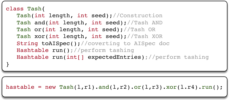
Tash framework. Our framework is developed by using Java language and the LLRP Toolkit(llr, 2010), which is an open-source library for handling ROSpec and AOSpec. Fig. 9(b) shows the primary interfaces provided by the tash framework. The class Tash makes the first selection through its construction method and allows the calls of three operators to be chained together in a single statement. The method toAISpec converts a Tash object or a chain of Tash objects into an AISpec. The entry-inventories are physically executed in the connected reader when the method run is invoked. This method allows users to make selective entry-inventories by passing an index array. For example, the operation can be coded in a manner similar to that shown at the bottom of Fig. 9(b).
| ImpinJ Monza | Alien ALN | |||||||||||||||||
| Commands | 5 | D | E | QT | X-2K | X-8K | R6 | R6-P | R6-C | 9840 | 9830 | 9662 | 9610 | 9726 | 9820 | 9715 | 9716 | 9629 |
| MemBank1 (bits) | 128 | 128 | 496 | 128 | 128 | 128 | 96 | 128/96 | 96 | 128 | 128 | 480 | 96-480 | 128 | 128 | 128 | 128 | 96 |
| MemBank3 (bits) | 32 | 32 | 128 | 512 | 2176 | 8192 | × | 32/64 | 32 | 128 | 128 | 512 | 512 | 128 | 128 | 128 | 128 | 512 |
| Write cmd | ✓ | ✓ | ✓ | ✓ | ✓ | ✓ | × | ✓ | ✓ | ✓ | ✓ | ✓ | ✓ | ✓ | ✓ | ✓ | ✓ | ✓ |
| Select cmd | ✓ | ✓ | ✓ | ✓ | ✓ | ✓ | ✓ | ✓ | ✓ | ✓ | ✓ | ✓ | ✓ | ✓ | ✓ | ✓ | ✓ | ✓ |
| Truncate cmd | – | – | – | – | – | – | – | – | – | – | – | – | – | – | – | – | – | – |
7. Microbenchmark
We start with a few experiments that provide insight to our hash primitives.
7.1. Experimental Setup

We evaluate the framework using COTS UHF readers and tags. We use a total of models of ImpinJ readers (R220, R420 and R680), each of which is connected to a MHz and dB gain directional antenna. In order to better understand the feasibility and effectiveness of Tash in practice, we test a total of COTS tags with different models. We divide these tags into groups of tags each. The tags of each group are densely attached to a plastic board which is placed in front of a reader antenna. As shown in Fig. 10, three hundreds is the maximum number of tags that can be covered by one directional antenna in our laboratory. We store the EPC numbers in our database as the ground truth. The 128-bit MD5 is employed as the common hash function to generate the hash values of EPCs. The experiments with the same settings are repeated across the groups, and the average result is reported.
7.2. Compatibility Investigation
First, we investigate the compatibility of Gen2 across different types of readers and different types of tags in terms of the functions or commands that Tash requires. The readers and tags may come from different manufacturers but work together in practice. These investigated products are all publicly claimed to be completely Gen2-compatible.
Reader compatibility. We investigate the R220, R420, and R680 models from ImpinJ(imp, 2017), the Mercury6, Sargas and M6e models from ThingMagic(thi, 2017), as well as the ALR-F800, 9900+, 9680 and 9650 models from Alien(ali, 2017). We perform the investigation through real tests for the first three models of readers (i.e., the ImpinJ series), and investigate the other readers through their data sheets or manuals (because we are limited by the lack of hardware). The Gen2-compatibility of readers is briefly summarized in Table. 4. Consequently, we have the subsequent findings. () All the readers do support Write/Read command, which Tash uses for writing or reading hash values of EPC numbers. () All the readers do support the Select command, which Tash uses for the selective reading. () However, our practical tests suggest that none model of the ImpinJ series supports the Truncate command, which Tash uses to hear the one-bit presence signal. The serviceability of other readers is not clearly indicated in the manuals of those readers. () The Gen2 protocol does not specify how many C1G2Filters and AISpecs that a reader should support. Our practical tests suggest that the ImpinJ series supports C1G2Filters and AISpecs, which means that we can only use a maximum of four tash operators each time.
| Commands or functions | ImpinJ | ThingMagic | Alien |
|---|---|---|---|
| Write/Read | ✓ | ✓ | ✓ |
| Select | ✓ | ✓ | ✓ |
| Truncate | × | – | – |
| Max No. of C1G2Filters | – | – | |
| Max No. of AISpecs | – | – |
Tag compatibility. We investigate chip models from ImpinJ Monza series and additional models from Alien ALN series. The majority of tags on the market contain these models of chips and customized antennas. Table. 3 summarizes the result of our investigation, from which we have the subsequent findings. (1) Tags reserve bits of memory for storing EPC numbers, among which the size of bits has become the de facto standard. (2) Tash requires MemBank-3 to store the hash values. The results of the investigation show that almost all tags allow to write to and read from the third memory bank, with an exception of ImpinJ Monza R6, which does not have the user-defined memory. The size of the third memory bank fluctuates around bits. The de facto standard has become bits. (4) All tags are claimed to support the Truncate command according to their public data sheets. However, we have no idea about their real serviceability due to the lack of Truncate-supportable reader available for practical tests. In our future work, we plan to utilize USRP for further tests.
Summary. Despite positive and public claims, our investigation shows that current COTS RFID devices, regardless of readers or tags and models, have some defects in their compatibility with Gen2, especially with regard to Truncate. The reason, we may infer, is that these commands are seldom used in practice and therefore never receive attention from manufacturers. The partial compatibility of such devices cannot fully achieve the performance Tash brings. Even so, we are obliged to make the claim, again, that our design strictly follows the Gen2 protocol. We hope this work can encourage manufacturers to upgrade their products (e.g., reader firmware) to achieve full compatibility.
7.3. Tash Function
Second, we evaluate the tash function with respect to the randomness and the accessibility.
Randomness. Randomness is the most important metric for a hash function. It requires that the outputs of a hash function must be uniformly distributed. To validate the randomness of the tash function, we collect real EPC numbers from our partner (i.e., an international logistics company), which introduced RFID technology for sorting tasks five years ago. Each EPC number has a length of bits and encodes the basic information about the package, such as sources, destinations, serial numbers, and so on. We employ the -bit MD5 to create the hash values of these EPCs. As the minimum size of the MemBank-3 is bits (see Table. 4), we choose to use only the first bits for our tests. We traverse and from and respectively. For each pair of and , we obtain tash values over all the EPCs. Across these tash values, we further conduct the following two analysis: (1) We merge tash values, which are randomly selected from the above results, into a long bit string. We then calculate the percents of ‘0’ and ‘1’ emerged in that bit string. This operation is repeated for times. Finally, totally pairs of percents are obtained. Their CDFs are plotted in Fig. 11(a). Ideally, each bit has a equal probability of to be zero or one if a hash function makes a good randomicity. From the figure, we can figure out that the percents distributed between and . In particular, percents of ‘0’ and ‘1’ have means of and with standard deviations of and respectively. (2) We shuffle these values into groups, and employ the -test with a significance level of to test each group’s goodness-of-fits of the uniform distribution (i.e., passed or failed). Then, we finally calculate the pass rate for a pair of setting. In this manner, we totally obtain pass rates. More than of the pass rates are over than . In particular, three sets of the results with , and and a variable , are selected to show in Fig. 11(b). We find that of the pass rates exceed for the three cases, and their median pass rates are around . Thus, the two above statistical results suggest that our tash function has a very good quality of randomness.
Accessibility. Accessibility refers to the ability to get access to a tash value from a tag. As aforementioned, we have two ways to acquire the tash values. The first way is to use the Read command. The second way is to indirectly access a tash value through a selective reading. We choose the second method since it is the basis of our design. Specifically, we perform a selective reading to determine whether the tags are collected as expected, when given random inputs and a possible tash value. We intensively and continuously perform such readings across the tags using three 4-port ImpinJ readers for three rounds of hours in a relatively isolated environment (e.g., an empty room without disturbance). Surprisingly, we find all the reading results faithfully conform to our benchmarks without any exceptions. This shows that the selective reading is well supported by the manufactures and is both stable and reliable.
7.4. Tash Table Function
Third, we evaluate the performance of the tash table function in terms of its balance and gathering speed.
Balance. A good hash table function will equally assign each key to a bucket. We expect the output tash table to be as balanced as possible. To show this feature, we generate different -bit tash tables (i.e., each includes entries) across tags using different random seeds. If the tash table is well balanced, the expected number of each entry should be very close to . Fig. 12(a) shows the mean number of tags in each entry as well as their standard deviations. The average number across entries equals , which is very close to the expected theoretical value. The average standard deviation equals . Thus, the good randomness quality of tash functions results in output tash tables being well balanced.
Gathering speed. We then consider the time consumption of gathering a tash table. Fixing the random seed, we vary the table dimension from to . We then measure the time taken on gathering a tash table with the deployed tags. Fig. 12(b) shows the resulting time as a function of the table dimension. From the immediately above-mentioned figure, we can observe the subsequent findings. () When without truncating reply, the result is equivalent to collecting complete EPCs of all the tags. Such time consumption (i.e., ) is viewed as our baseline. () By contrast, when without truncating a reply, the collection amounts to dividing all the tags into groups “equally” and then collecting each group independently. In this manner, when , such “divide and conquer” approach is better than “one time deal”, i.e., a drop in overhead of about . The Gen2 reader uses a Q-adaptive algorithm for the anti-collision. This algorithm is able to adaptively learn the best frame length from the collision history. Due to the division, a smaller number of tags can make reader’s learning relatively quicker and improve the overall performance. () However, when , the performance of “divide and conquer” approach starts to deteriorate. The ImpinJ reader supports AISpecs at most (see Table. 4). We have to re-send another ROSpec for the remaining selective readings when the number of entry-inventory is above (i.e., ), which introduces additional time consumption. () We then consider the case where the reply is truncated to a one-bit presence signal as assumed by HEPs. Due to the defects of ImpinJ readers in the implementation of the Truncate command, we cannot measure the actual time spent on collecting truncated EPCs. We can only utilize the least-square algorithm to estimate the transmission time for a one-bit presence signal. Our fitting results show that truncating reply would introduce about drop of the overhead at least.
7.5. Tash Operators
Finally, we investigate the performance of tash operators. Superior to existing HEPs, these operators allow us to perform set operations on-tag and conduct a one-stop inventory. In particular, we show the performance of OR as a representative across tags. The tests for other operators are similar and omitted due to the space limitation. In the experiments, we fix the two random seeds but change the dimension of tash table. Fig. 13 shows the results of three cases. In Case , we independently produce tash tables without truncating a reply and conduct the OR in the application layer. In Case and Case , we conduct on-tag OR function as Tash provides without and with truncating a reply respectively. Consequently, when the dimension equals , Case 1 takes on collecting two tables. On the contrary, the amount of time taken is reduced to (i.e., drop) if we perform an on-tag OR function even without truncation (Case 2). Ideally, the amount of time taken could be further reduced to by using a truncating reply (Case 3), which offers a staggering drop in time usage by . Our experiments relate only to the amount of time spent on ORing two tables. It may be predicted that much more outperformance will be gained if multiple tables are involved. The tash operators that we design in this work have never been proposed before.
8. Usage Evaluation
We then use our prototype to demonstrate the benefits and potentials of Tash in two typical applications.
8.1. Usage I: Cardinality Estimation
We evaluate our estimation scheme through the testbed as well as large-scale simulations.
Testbed based. Our scheme only uses the first entry of the tash table for the estimation, thereby we only need one entry-inventory. Fig. 14(a) shows the CDF of estimation results across tags. We define the error rate as where is the estimated number. As a result, of the estimations have an error rate less than and a median of when setting the dimension . In this case, almost half tags follow into the first entry so the rate could be pretty high, at the price of longer inventory time. As increases, the error rate also increases because less samples are acquired for the estimation. These experiments show the feasibility of using tash table for cardinality estimation.
Simulation based. We then perform the evaluation through large-scale simulations for two reasons: () ensuring its scalability when meeting a huge number of tags. () making comparisons with prior work, which are all simulation-based. We numerically simulate in Matlab using tash scheme as well as other five prior RFID estimation schemes: UPE(Kodialam and Nandagopal, 2006), EZB(Kodialam et al., 2007), FNEB(Han et al., 2010), MLE(Li et al., 2010b), ART(Shahzad and Liu, 2012). We implement these schemes by referring to the RFID estimation tool developed by Shahzad(Shahzad, [n. d.]). Fig. 14(b) shows the time cost with a varying given and . We observe that our scheme is faster than the others on average when . Thus our scheme is suitable for the estimation with a small number of tags. When , the performance of our scheme starts to vibrate between ART and MLE, due to two reasons. First, our scheme is not collision-free so that more efforts are required to deal with the collisions incurred by more tags. Second, the size of a tash table can only increase in the power of two, making the size always vibrate around the optimal one. Even so, the advantage of our scheme is still clear: it is the first RFID estimation scheme that can work in real life. Notice that ART claimed to work with RFID systems because they are theoretically compatible with ALOHA protocols. Actually, the current COTS RFID systems do not allow user to control the low-level access, like fined-grained adjustment of frame length and obtaining slot-level feedback, which are necessary to implement ART. Thus, there is no way for ART to implement their algorithms over COTS RFID systems without any hardware modification and fabrication.
8.2. Usage II: Missing Detection
Finally, we evaluate the effectiveness of missing detection in real case. We randomly remove tags from the testbed. Since we only have tags in total, we fix the number of random seeds to , i.e., . The performance is evaluated in term of the false positive rate (FPR), which is the ratio of number of mistakenly detected as missing tags to the total number of really missing tags. Our scheme is able to successfully find out all the missing tags because the residual table always contains the entries that missing tags are tashed into. Fig. 15(a) shows the results of the first case in which we use an -bit hash table (i.e., ) to detect the missing tags. Consequently, the FPR is maintained around when (i.e., of the tags are missing). Fig. 15(b) shows the second case in which we remove tags and detect the missing tags by changing the dimension of tash table. As Theorem. 2 suggests, we should set to guarantee the FPR . From the figure, we can find that the results of our experiments completely conform to this theorem. The real FPRs equal and in the three cases. Tash enabled missing detection works well in practice.
9. Conclusion
This work discusses a fundamental issue that how to supplement hash functionality to existing COTS RFID systems, which is dispensable for prior HEPs. A key innovation of this work is our design of hash primitives, which is implemented using selective reading. Tash not only makes a big step forward in boosting prior HEPs, but also opens up a wide range of exciting opportunities.
Acknowledgments
The research is supported by GRF/ECS (NO. 25222917), NSFC General Program (NO. 61572282) and Hong Kong Polytechnic University (NO. 1-ZVJ3). We thank all the reviewers for their valuable comments and helpful suggestions, and particularly thank Eric Rozner for the shepherd.
References
- gen (2004) 2004. EPCglobal Gen2 Specification. www.gs1.org/epcglobal. (2004).
- llr (2010) 2010. LLRP Toolkit. http://llrp.org. (2010).
- ali (2017) 2017. Alien. http://www.alientechnology.com. (2017).
- imp (2017) 2017. ImpinJ, Inc. http://www.impinj.com/. (2017).
- thi (2017) 2017. ThingMagic. http://www.thingmagic.com. (2017).
- Bogdanov et al. (2007) Andrey Bogdanov, Lars R Knudsen, Gregor Leander, Christof Paar, Axel Poschmann, Matthew JB Robshaw, Yannick Seurin, and Charlotte Vikkelsoe. 2007. PRESENT: An ultra-lightweight block cipher. In CHES, Vol. 4727. Springer, 450–466.
- Bogdanov et al. (2008) Andrey Bogdanov, Gregor Leander, Christof Paar, Axel Poschmann, Matt JB Robshaw, and Yannick Seurin. 2008. Hash functions and RFID tags: Mind the gap. In Proc. of IACR CHES.
- Broder and Mitzenmacher (2004) Andrei Broder and Michael Mitzenmacher. 2004. Network applications of bloom filters: A survey. Internet Mathematics 1, 4 (2004), 485–509.
- Chen et al. (2013) Binbin Chen, Ziling Zhou, and Haifeng Yu. 2013. Understanding RFID counting protocols. In Proc. of ACM MobiCom.
- Dobkin (2012) Daniel M Dobkin. 2012. The RF in RFID: UHF RFID in Practice. Newnes.
- Feldhofer et al. (2004) Martin Feldhofer, Sandra Dominikus, and Johannes Wolkerstorfer. 2004. Strong authentication for RFID systems using the AES algorithm. In CHES, Vol. 4. Springer, 357–370.
- Feldhofer and Rechberger (2006) Martin Feldhofer and Christian Rechberger. 2006. A case against currently used hash functions in RFID protocols. In On the move to meaningful internet systems 2006: OTM 2006 workshops. Springer, 372–381.
- Frost and Sullivan (2011) Frost and Sullivan. 2011. Global RFID healthcare and pharmaceutical marke. Industry Report (2011).
- Gong et al. (2014) Wei Gong, Kebin Liu, Xin Miao, and Haoxiang Liu. 2014. Arbitrarily accurate approximation scheme for large-scale rfid cardinality estimation. In Proc. of IEEE INFOCOM.
- Good and Benaissa (2007) Tim Good and Mohammed Benaissa. 2007. Hardware results for selected stream cipher candidates. State of the Art of Stream Ciphers 7 (2007), 191–204.
- Han et al. (2010) Hao Han, Bo Sheng, Chiu C Tan, Qun Li, Weizhen Mao, and Sanglu Lu. 2010. Counting RFID tags efficiently and anonymously. In Proc. of IEEE INFOCOM.
- Hong et al. (2006) Deukjo Hong, Jaechul Sung, Seokhie Hong, Jongin Lim, Sangjin Lee, Bonseok Koo, Changhoon Lee, Donghoon Chang, Jesang Lee, Kitae Jeong, et al. 2006. HIGHT: A new block cipher suitable for low-resource device. In CHES, Vol. 4249. Springer, 46–59.
- Hou et al. (2015) Yuxiao Hou, Jiajue Ou, Yuanqing Zheng, and Mo Li. 2015. PLACE: Physical layer cardinality estimation for large-scale RFID systems. In Proc. of IEEE INFOCOM.
- Kodialam and Nandagopal (2006) Murali Kodialam and Thyaga Nandagopal. 2006. Fast and reliable estimation schemes in RFID systems. In Proc. of ACM MobiCom.
- Kodialam et al. (2007) Murali Kodialam, Thyaga Nandagopal, and Wing Cheong Lau. 2007. Anonymous tracking using RFID tags. In Proc. of IEEE INFOCOM.
- Li et al. (2016) Binbin Li, Yuan He, Wenyuan Liu, Lin Wang, and Hongyan Wang. 2016. LocP: An efficient Localized Polling Protocol for large-scale RFID systems. In Proc. of IEEE ICNP.
- Li et al. (2010a) Tao Li, Shigang Chen, and Yibei Ling. 2010a. Identifying the missing tags in a large RFID system. In Proc. of ACM MobiHoc.
- Li et al. (2013) Tao Li, Shigang Chen, and Yibei Ling. 2013. Efficient protocols for identifying the missing tags in a large RFID system. IEEE/ACM Transactions on Networking 21, 6 (2013), 1974–1987.
- Li et al. (2010b) Tao Li, Samuel Wu, Shigang Chen, and Mark Yang. 2010b. Energy efficient algorithms for the RFID estimation problem. In Proc. of IEEE INFOCOM.
- Lim and Korkishko (2005) Chae Hoon Lim and Tymur Korkishko. 2005. mCrypton-a lightweight block cipher for security of low-cost RFID tags and sensors. In WISA, Vol. 3786. Springer, 243–258.
- Liu et al. (2014a) Haoxiang Liu, Wei Gong, Xin Miao, Kebin Liu, and Wenbo He. 2014a. Towards adaptive continuous scanning in large-scale rfid systems. In Proc. of IEEE INFOCOM.
- Liu et al. (2015a) Jia Liu, Bin Xiao, Shigang Chen, Feng Zhu, and Lijun Chen. 2015a. Fast RFID grouping protocols. In Proc. of IEEE INFOCOM. 1948–1956.
- Liu et al. (2014b) Xiulong Liu, Keqiu Li, Geyong Min, Yanming Shen, Alex X Liu, and Wenyu Qu. 2014b. A multiple hashing approach to complete identification of missing RFID tags. IEEE Transactions on Communications 62, 3 (2014), 1046–1057.
- Liu et al. (2014c) Xiulong Liu, Keqiu Li, Heng Qi, Bin Xiao, and Xin Xie. 2014c. Fast counting the key tags in anonymous RFID systems. In Proc.of IEEE ICNP.
- Liu et al. (2015b) Xiulong Liu, Bin Xiao, Keqiu Li, Jie Wu, Alex X Liu, Heng Qi, and Xin Xie. 2015b. RFID cardinality estimation with blocker tags. In Proc. of IEEE INFOCOM.
- Liu et al. (2015c) Xuan Liu, Bin Xiao, Shigeng Zhang, Kai Bu, and Alvin Chan. 2015c. STEP: A time-efficient tag searching protocol in large RFID systems. IEEE Trans. Comput. 64, 11 (2015), 3265–3277.
- Luo et al. (2011) Wen Luo, Shigang Chen, Tao Li, and Shiping Chen. 2011. Efficient missing tag detection in RFID systems. In Proc. of IEEE INFOCOM.
- Luo et al. (2012) Wen Luo, Shigang Chen, Tao Li, and Yan Qiao. 2012. Probabilistic missing-tag detection and energy-time tradeoff in large-scale RFID systems. In Proc. of ACM MobiHoc.
- Luo et al. (2014) Wen Luo, Shigang Chen, Yan Qiao, and Tao Li. 2014. Missing-tag detection and energy–time tradeoff in large-scale RFID systems with unreliable channels. IEEE/ACM Transactions on Networking 22, 4 (2014), 1079–1091.
- Luo et al. (2013) Wen Luo, Yan Qiao, and Shigang Chen. 2013. An efficient protocol for RFID multigroup threshold-based classification. In Proc. of IEEE INFOCOM. 890–898.
- Luo et al. (2016) Wen Luo, Yan Qiao, Shigang Chen, and Min Chen. 2016. An efficient protocol for RFID multigroup threshold-based classification based on sampling and logical bitmap. IEEE/ACM Transactions on Networking 24, 1 (2016), 397–407.
- Ma et al. (2012) Cunqing Ma, Jingqiang Lin, and Yuewu Wang. 2012. Efficient missing tag detection in a large RFID system. In Proc. of IEEE TrustCom.
- Pendl et al. (2012) Christian Pendl, Markus Pelnar, and Michael Hutter. 2012. Elliptic curve cryptography on the WISP UHF RFID tag. RFID. Security and Privacy (2012), 32–47.
- Philipose et al. (2005) Matthai Philipose, Joshua R Smith, Bing Jiang, Alexander Mamishev, Sumit Roy, and Kishore Sundara-Rajan. 2005. Battery-free wireless identification and sensing. IEEE Pervasive computing 4, 1 (2005), 37–45.
- Poschmann et al. (2007) Axel Poschmann, Gregor Leander, Kai Schramm, and Christof Paar. 2007. New Lightweight DES Variants Suited for RFID Applications. In FSE, Vol. 4593. 196–210.
- Qian et al. (2010) Chen Qian, Yunhuai Liu, Hoilun Ngan, and Lionel M Ni. 2010. Asap: Scalable identification and counting for contactless rfid systems. In Proc. of IEEE ICDCS.
- Qian et al. (2011) Chen Qian, Hoilun Ngan, Yunhao Liu, and Lionel M Ni. 2011. Cardinality estimation for large-scale RFID systems. IEEE Transactions on Parallel and Distributed Systems 22, 9 (2011), 1441–1454.
- Qiao et al. (2013) Yan Qiao, Shigang Chen, and Tao Li. 2013. Tag-ordering polling protocols in RFID systems. In RFID as an Infrastructure. Springer, 59–82.
- Qiao et al. (2011) Yan Qiao, Shigang Chen, Tao Li, and Shiping Chen. 2011. Energy-efficient polling protocols in RFID systems. In Proc. of ACM MobiHoc.
- Rolfes et al. (2008) Carsten Rolfes, Axel Poschmann, Gregor Leander, and Christof Paar. 2008. Ultra-lightweight implementations for smart devices–security for 1000 gate equivalents. In CARDIS, Vol. 5189. Springer, 89–103.
- Shah-Mansouri and Wong (2011) Vahid Shah-Mansouri and Vincent WS Wong. 2011. Cardinality estimation in RFID systems with multiple readers. IEEE Transactions on Wireless Communications 10, 5 (2011), 1458–1469.
- Shahzad ([n. d.]) Muhammad Shahzad. [n. d.]. RFID estimation tool. http://www4.ncsu.edu/~mshahza/publications.html. ([n. d.]).
- Shahzad and Liu (2012) Muhammad Shahzad and Alex X Liu. 2012. Every bit counts: fast and scalable RFID estimation. In Proc. of ACM MobiCom.
- Shahzad and Liu (2015) Muhammad Shahzad and Alex X Liu. 2015. Expecting the unexpected: Fast and reliable detection of missing RFID tags in the wild. In Proc. of IEEE INFOCOM.
- Shahzad and Liu (2016) Muhammad Shahzad and Alex X Liu. 2016. Fast and Reliable Detection and Identification of Missing RFID Tags in the Wild. IEEE/ACM Transactions on Networking 24, 6 (2016), 3770–3784.
- Sheng et al. (2010) Bo Sheng, Qun Li, and Weizhen Mao. 2010. Efficient continuous scanning in RFID systems. In Proc. of IEEE INFOCOM.
- Sheng et al. (2008) Bo Sheng, Chiu Chiang Tan, Qun Li, and Weizhen Mao. 2008. Finding popular categories for RFID tags. In Proc. of ACM MobiHoc.
- Sze et al. (2009) W-K Sze, W-C Lau, and O-C Yue. 2009. Fast RFID counting under unreliable radio channels. In Proc. of IEEE ICC.
- Tan et al. (2008) Chiu C Tan, Bo Sheng, and Qun Li. 2008. How to monitor for missing RFID tags. In Proc. of IEEE ICDCS.
- Tan et al. (2010) Chiu C Tan, Bo Sheng, and Qun Li. 2010. Efficient techniques for monitoring missing RFID tags. IEEE Transactions on Wireless Communications 9, 6 (2010), 1882–1889.
- Wang et al. (2012) Jue Wang, Haitham Hassanieh, Dina Katabi, and Piotr Indyk. 2012. Efficient and reliable low-power backscatter networks. In Proc. of ACM SIGCOM. ACM, 61–72.
- Xiao et al. (2013) Qingjun Xiao, Bin Xiao, and Shigang Chen. 2013. Differential estimation in dynamic RFID systems. In Proc. of IEEE INFOCOM.
- Xie et al. (2014a) Lei Xie, Hao Han, Qun Li, Jie Wu, and Sanglu Lu. 2014a. Efficiently collecting histograms over rfid tags. In Proc. of IEEE INFOCOM.
- Xie et al. (2013) Lei Xie, Qun Li, Xi Chen, Sanglu Lu, and Daoxu Chen. 2013. Continuous scanning with mobile reader in RFID systems: An experimental study. In Proc. of ACM MobiHoc. ACM, 11–20.
- Xie et al. (2014b) Wei Xie, Lei Xie, Chen Zhang, Qiang Wang, Jian Xu, Quan Zhang, and Chaojing Tang. 2014b. RFID seeking: Finding a lost tag rather than only detecting its missing. Journal of Network and Computer Applications 42 (2014), 135–142.
- Yang et al. (2014) Lei Yang, Yekui Chen, Xiang-Yang Li, Chaowei Xiao, Mo Li, and Yunhao Liu. 2014. Tagoram: real-time tracking of mobile RFID tags to high precision using COTS devices. In Proc. of ACM MobiCom.
- Yang et al. (2016) Lei Yang, Yao Li, Qiongzheng Lin, Xiang-Yang Li, and Yunhao Liu. 2016. Making sense of mechanical vibration period with sub-millisecond accuracy using backscatter signals. In Proc. of ACM MobiCom.
- Yoshida et al. (2007) Hirotaka Yoshida, Dai Watanabe, Katsuyuki Okeya, Jun Kitahara, Hongjun Wu, Özgül Küçük, and Bart Preneel. 2007. MAME: A compression function with reduced hardware requirements. In International Workshop on Cryptographic Hardware and Embedded Systems. Springer, 148–165.
- Yu et al. (2015) Jihong Yu, Lin Chen, and Kehao Wang. 2015. Finding Needles in a Haystack: Missing Tag Detection in Large RFID Systems. arXiv preprint arXiv:1512.05228 (2015).
- Yu et al. (2016) Jihong Yu, Lin Chen, Rongrong Zhang, and Kehao Wang. 2016. On Missing Tag Detection in Multiple-group Multiple-region RFID Systems. IEEE Transactions on Mobile Computing (2016).
- Yu et al. ([n. d.]) Y Yu, Y Yang, Y Fan, and H Min. [n. d.]. Security Scheme for RFID Tag: Auto-ID Labs white paper WP-HARDWARE-022. http://www.autoidlabs.org/. ([n. d.]).
- Zhang et al. (2011a) Hong Zhang, Jeremy Gummeson, Benjamin Ransford, and Kevin Fu. 2011a. Moo: A batteryless computational RFID and sensing platform. University of Massachusetts Computer Science Technical Report UM-CS-2011-020 (2011).
- Zhang et al. (2011b) Rui Zhang, Yunzhong Liu, Yanchao Zhang, and Jinyuan Sun. 2011b. Fast identification of the missing tags in a large RFID system. In Proc. of IEEE SECON.
- Zhang et al. (2009) Yan Zhang, Laurence T Yang, and Jiming Chen. 2009. RFID and sensor networks: architectures, protocols, security, and integrations. CRC Press.
- Zheng and Li (2013a) Yuanqing Zheng and Mo Li. 2013a. Fast tag searching protocol for large-scale RFID systems. IEEE/ACM Transactions on Networking 21, 3 (2013), 924–934.
- Zheng and Li (2013b) Yuanqing Zheng and Mo Li. 2013b. ZOE: Fast cardinality estimation for large-scale RFID systems. In Proc. of IEEE INFOCOM.
- Zheng and Li (2014) Yuanqing Zheng and Mo Li. 2014. Towards more efficient cardinality estimation for large-scale RFID systems. IEEE/ACM Transactions on Networking 22, 6 (2014), 1886–1896.
- Zheng and Li (2015) Yuanqing Zheng and Mo Li. 2015. P-mti: Physical-layer missing tag identification via compressive sensing. IEEE/ACM Transactions on Networking 23, 4 (2015), 1356–1366.