Phase Space Analysis of the Accelerating Multi-fluid Universe
Abstract
We study in detail the phase space of a Friedmann-Robertson-Walker Universe filled with various cosmological fluids which may or may not interact. We use various expressions for the equation of state, and we analyze the physical significance of the resulting fixed points. In addition we discuss the effects of the stability or an instability of some fixed points. Moreover we study an interesting phenomenological scenario for which there is an oscillating interaction between the dark energy and dark matter fluid. As we demonstrate, in the context of the model we use, at early times the interaction is negligible and it starts to grow as the cosmic time approaches the late-time era. Also the cosmological dynamical system is split into two distinct dynamical systems which have two distinct de Sitter fixed points, with the early-time de Sitter point being unstable. This framework gives an explicit example of the unification of the early-time with late-time acceleration. Finally, we discuss in some detail the physical interpretation of the various models we present in this work.
pacs
04.50.Kd, 95.36.+x, 98.80.-k, 98.80.Cq, 11.25.-wI Introduction
In modern theoretical cosmology, the most striking event was the observation of the late-time acceleration [1] that our Universe undergoes at present time. Admittedly this observation has utterly changed the way of thinking of modern cosmologists, since this late-time acceleration is a feature of our Universe that was never thought it would actually occur. Consequently, the focus for the last nearly 20 years is to model in a successful way this late-time acceleration and also to harbor the late and early-time acceleration era in a unified theoretical framework. Towards this unified description, many proposals, especially those suggesting to modify the gravitational sector, have been introduced ever since, see the reviews [2, 3, 4, 5] for details. From the first moment that the late-time acceleration has been observed, it was realized that no perfect matter fluid known at that time was able to realize the late-time acceleration era, and therefore the need for alternative generalized cosmological fluids was compelling. By using generalized cosmological fluids, both the late and early-time acceleration era can be realized, and up to date there are many theoretical proposals that use generalized fluids, for example in Refs. [6, 7, 8, 9, 10, 11, 12] imperfect fluids are used in order to describe the cosmological evolution of our Universe, and in some cases certain particular examples are used, called viscous fluids are (see [13] for reviews). It is notable that the imperfect fluids may describe even phantom evolution of our Universe, without using phantom scalar fields, which violate the energy conditions, see Refs. [6, 8] for details. Furthermore, other cosmological evolutions like bouncing cosmology, in the context of both classical and loop quantum cosmology imperfect fluids were studied in [14], and also singular cosmology can be realized by imperfect fluids [15, 16]. Furthermore, several models which take into account bulk viscosity were discussed in Refs. [17, 18, 19, 20, 21, 22, 23, 24, 25, 26, 27, 28, 29], and also an important class of models which assume an interaction between dark matter and dark energy fluids, can be found in Refs. [17, 30, 31].
In this paper we shall perform a detailed phase-space analysis of a Friedmann-Robertson-Walker Universe, filled with different fluid components, which may or may not interact between them. The dynamical evolution of such kind of model is described by the Friedmann equations,
| (1) |
| (2) |
or equivalently,
| (3) |
and also the energy conservation equations hold true,
| (4) |
In the above, and also the equation of state (EoS) may be highly non-trivial for some fluid components. We shall appropriately choose the variables in order to capture the phase space dynamics in the most optimal way, and we shall analyze the structure of the phase space by providing an analytic treatment of the cosmological dynamical equations. Seeing the cosmological equations as a dynamical system is a particularly appealing way to investigate the phase space in many cosmological contexts, see for example [32, 33, 34, 35, 36, 37], but also in modified gravity too, see for example [38, 39, 40, 41, 42, 43, 44, 45, 46, 47]. In most cases, the choice of the dynamical system variables plays a crucial choice, and in some cases the resulting cosmological dynamical system may be rendered autonomous [48]. Also it is possible to choose dimensionless variables, see for example Refs. [39, 40] for an gravity cosmological dynamical system, and also see Ref. [49], for a cosmological theory with higher derivatives of the scalar curvature. The dynamical systems approach for cosmological systems has many attributes, with the most important being the fact that the fixed points of the dynamical system actually provide new insights with regards to the behavior of the attractor solutions and also reveals the stability structure of the dynamical system near the attractors. It is conceivable that the choice of the variables plays an important role, as we also demonstrate by this work.
This paper is organized as follows: In section II we present some well known features of dynamical systems approach in cosmological context with generalized fluids, in section III we discuss in brief how interactions between dark matter and dark energy may be introduced and by using appropriately chosen variables we present how the dynamical systems analysis can be performed in this case. In section IV we generalize the formalism we developed in the previous sections and by using dimensionless variables, we investigate the physical consequences of having various equations of state for the fluid components of the cosmological system. In section V by using appropriately chosen dimensionless variables, we investigate in detail how the interaction of dark matter and dark energy fluids may affects the phase space structure. We study the stability and behavior of the fixed points of the dynamical system and we also discuss how the early and late-time acceleration eras are affected by the various functional forms of the interaction coupling between dark matter and dark energy. Finally the conclusions follow in the end of the paper.
II Standard Approach on Dynamical Systems and Cosmological Dynamics
In this section we present the simplest case of the dynamical systems approach in cosmological dynamics. We consider the simplest case in which the Universe is filled with radiation and a perfect fluid with a non-trivial EoS of the form [50]. Such non-trivial EoS can be considered as some sort of viscous fluid or generalized EoS fluid, see [51] for a review on this topic. In addition, such an EoS can be considered as an effective fluid presentation of some modified gravity theory [3, 4]. In the case at hand, the full dynamical system takes the following form,
| (5) | |||||
| (6) | |||||
| (7) |
The appearance of the term might seem unconventional, from a thermodynamic point of view, and we need to briefly describe the motivation for using such a term. This term encompasses the viscous part of the cosmological fluid, so it mainly quantifies the viscosity of the fluid. In the Universe, nd especially in the very early stages of it’s evolution, the effects of a viscous cosmological component are most likely expected to occur during the neutrino decoupling process, which occurs at the end of the lepton era [52]. Hence, viscosity is encompassed in the very own fabric of the Universe. In addition, a strong motivation for using viscous fluid components comes from the fact that the perfect fluid approach among cosmologists-hydrodynamicists is just an ideal approach, and does not describe the real world. Finally, due to the fact that early and late-time acceleration may be described by an unknown form of a cosmological fluid, it is natural to assume that the fluid has the most general form, which means that a viscous component is needed11 1 Note that terms of the form in the cosmological relation between the effective pressure and the energy density, naturally occur in modified gravity thermodynamics [53].
Having described the motivation for the use of viscous fluid components, we can rewrite the above cosmological equations in terms of dimensionless variables. In the case at hand, there is only one independent variable due to the constraint equation (5). By using the -foldings number22 2 In this case time derivatives for some variable transform as and by introducing a new dimensionless variable defined as,
we obtain the next dynamical equation,
| (8) |
where the variables , and must be expressed in terms of depending on the choices of the functions and .
Let us here discuss the simplest choice of EoS, which is , which implies that and . It is easy to see that in this case, Eq. (8) takes the following form,
| (9) |
where the “prime” denotes differentiation with respect to the -foldings number. The equation that determines the stationary points for the above dynamical equation, is quadratic with discriminant , so the existing solutions are always real. For the case there is the only one solution, which is, . For the case there are two solutions, which are:
| (10) | |||||
| (11) |
and this case is the most interesting, since it provides us plenty dynamical solutions. Now note that the physical values that the variable can take, are , but for we have , which give us the following restrictions for the free parameters:
| (12) | |||
| (13) |
Let us study the stability conditions of the existing stationary points. It is clear that for every point there is only one eigenvalue , and for the fixed points at hand, we have,
| (14) | |||||
| (15) |
Therefore, we find that for any values of parameters , one of the fixed points is stable and the other one is unstable. Note that for the case we have and therefore it is compelling to investigate the corresponding center manifold, but fortunately this is not interesting case from a physical point of view. The physical significance of the stationary point is that it corresponds to a Universe with and . With regard to the fixed point , it corresponds to a Universe with some fixed relation between and .
III Models with Dark Matter Interacting to Dark Energy
Let us discuss at this point some models which describe interactions of dark matter with dark energy. The dynamical system in this case can be written in the following form,
| (16) | |||||
| (17) | |||||
| (18) | |||||
| (19) |
where the prime denotes as previously differentiation with respect to the -foldings number , and quantifies the interaction between dark energy and dark matter, and the term corresponds to the bulk viscous pressure of the dark matter fluid.
We will assume that the bulk viscous coefficient has the following form [17, 54, 55],
| (20) |
The motivation for using this kind of ansatz, comes from astronomical estimates on the relation between and , which was studied in Ref. [56], where a general form of the relation was assumed, and it was of the form . The choice we used in Eq. (20) yields a good fit between astronomical constraints and the fluid approach.
In this case we introduce the following set of dimensionless variables,
| (21) | |||||
| (22) | |||||
| (23) |
where only and are independent dynamical variables. By using the set of dimensionless variables, the dynamical equations (16)-(19) take the form33 3 Note that the constraint (16) and the equation for are already took into account in this system.:
| (24) | |||||
| (25) |
and by using the EoS we used in the previous section, namely, , we obtain,
| (26) | |||||
| (27) |
We can easily find the stationary points for the above dynamical system, by multiplying (24) by , (25) by and by combining the resulting equations we find,
| (28) |
The above equation indicates that there exist at most three stationary points, and it is clear that even in the most general case, the stationary points may be found analytically, and these are equal to,
| (29) |
| (30) |
Since there are a many free parameters, we investigate some particular cases, which are interesting from a physical point of view. We start off with the case , in which case the first fixed point takes the form,
| (31) |
and the corresponding eigenvalues are,
| (32) | |||||
| (33) |
Accordingly, the second fixed point is,
| (34) |
and the corresponding eigenvalues are,
| (35) | |||||
| (36) |
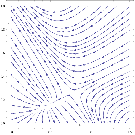
so the first point always unstable, whereas the second one may be stable, depending on the choice of the free parameters. However, if the first point lies in the physically allowed region, the second fixed point is rendered always unstable. Typical phase portrait with the two fixed points in the physical region, are presented in Fig.1.
Now let us consider another physically interesting case, for which . In this case, there exist three fixed points which are,
| (37) | |||||
| (38) | |||||
| (39) |
A particularly interesting subcase of the above is if we further choose, , then the fixed points become,
| (40) | |||||
| (41) | |||||
| (42) |
We can see that two fixed points are always unstable, whereas one of the three, the first or the second one depending on the sign of the parameter , is stable.
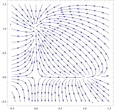
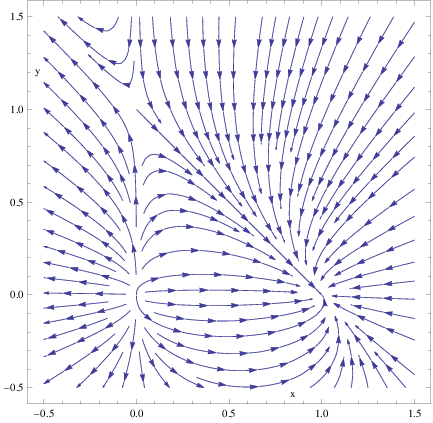
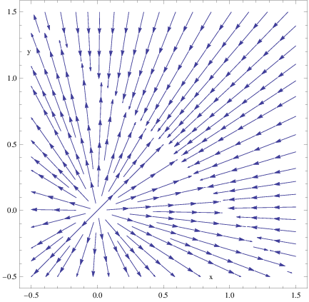
In Fig. 2 we plotted the phase portrait for the case , while in Fig. 3 we plotted the phase portrait for , and finally in Fig. 4 we can see the phase portrait for . As it can be seen in all figures, two of the three fixed points are unstable and one of the three is stable. Furthermore, it can be seen that by using Eq. (30), it is possible to find the case (by appropriately choosing the parameters) for which there will be some stationary point with fixed relation . This task may be solved numerically but we refrain from going into details on this.
IV Generalized Form of Cosmological Fluids
In this section we extend the cases we presented in section II to include generalized form of the EoS. We consider the simplest scenario for which the Universe is filled with and a perfect fluid with non-trivial EoS [50]. In this case, the dynamical system takes the following form,
| (43) | |||||
| (44) | |||||
| (45) | |||||
| (46) |
By using the -foldings number as independent variable and also by introducing the dimensionless variables,
the dynamical system can be cast in the following form,
| (47) | |||||
| (48) |
where according to the definition, and . Moreover we can see from the system (47)-(48) that the fixed point always exists, except for some very special choices of functions and .
It is interesting to note that actually due to the constraint equation (43), in the case at hand, there is only one independent variable, but by introducing the variable and by taking into account the equation (44), allows us to obtain more information about the evolution of the dynamical system. For instance, one of the most hard tasks in such kind of dynamical systems analysis, is to interpret correctly the physical meaning of the stationary points. This approach was firstly proposed in Ref. [57]. Let us introduce an additional parameter, which will be very helpful for this interpretation, which is the effective equation of state, which we denote as , and it is defined as follows:
| (49) |
The parameter can be expressed in terms of the dimensionless variables (43)-(44) as follows,
| (50) |
By specifying the EoS, it is possible to obtain various physically interesting evolution scenarios, so in the rest of this section we shall specify the EoS and we study in detail the dynamical evolution stemming from the choice of EoS.
IV.1 A Simplified Form of EoS
Let us discuss the simplest case of EoS, which is , which in turn implies , . It is easy to verify that in this case, the equations (47)-(48) take the following form,
| (51) | |||||
| (52) |
Thus we have the following stationary points for the dynamical system above,
- •
First fixed point .
- •
Second fixed point .
For the first fixed point we need to note that, this point lies in the physical region only if . The corresponding eigenvalues are , and . Using Eq. (50) we find that at this point we have .
With regard to the second fixed point, the eigenvalues are , and . Correspondingly we find that at this point . Thus we can see that the first fixed point always unstable and also that the second fixed point may be stable only if one (or both) of parameters , are strictly negative. For instance if we require that the first point lies in the physical region, we find that the second point is stable for . In Figs. (5-6) we plot the typical behavior of the phase trajectories.
Particularly, Fig. 5 corresponds to , and . The left fixed point corresponds to the effective EoS parameter and for the right fixed point, we have . Clearly the left fixed point represents radiation, while the right one corresponds to some phantom evolution. In Fig. 6, the phase portrait corresponds to the following choices for the parameters, , . The left point corresponds to an effective EoS parameter , while the right point corresponds to , which describes a form of collisional matter [58].
IV.2 More Complicated Forms of the EoS
Now let us study more complicated forms of the EoS, and we choose it to be of the form . This EoS is known to lead the cosmological system to finite-time singularities, as this was demonstrated in Ref. [50]. For this EoS, the equations (47)-(48) take the form,
| (53) | |||||
| (54) |
Correspondingly, the effective EoS in this case reads,
| (55) |
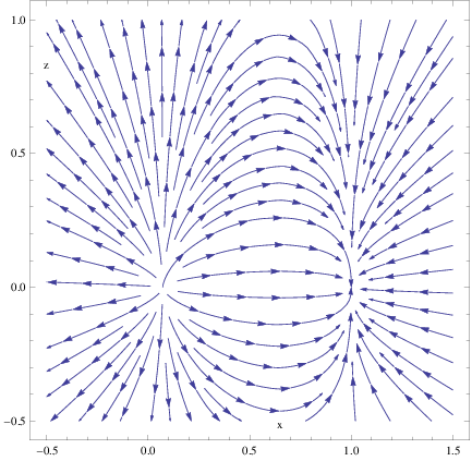
It is clear that in the most general case, this system may be solved only numerically, so let study some appropriately chosen cases which admit analytical solutions. Consider first the case for which , , in which case, the dynamical system (53)-(54) takes the following form,
| (56) | |||||
| (57) |
In this case there are two stationary points: the first is , 44 4 Note here that in all these three cases existence of the point , is not an obvious solution, but it can be confirmed by numerical investigations. and the second is , . For the first point, we have 55 5 Infinite values of looks like the Ruzmaikin solution at . and for the second one we have .
We can see that the second point corresponds to some new non-trivial de Sitter state with and . The eigenvalues of the second fixed point are , and . The typical behavior of the phase trajectories corresponding to this case, can be found in Fig.7, for , and . As it can be seen, there exist trajectories which start from the first fixed point , (note that zero values of correspond to infinite values of , which indicates a singularity) and end up to the second fixed point, with non-singular and non-zero values of . In effect, the second fixed point may be interpreted as a late-time acceleration de Sitter point of the cosmological dynamical system.
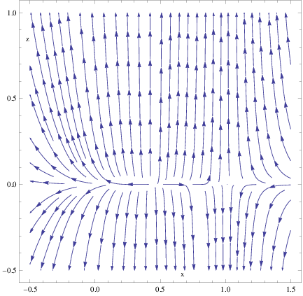
Now let us consider the case for which , and , in which case, the dynamical system (53)-(54) takes the form,
| (58) | |||||
| (59) |
In this case there are two stationary points, namely, , and also , and the situation is very similar to the previous case. For the first fixed point we have and for the second one . The eigenvalues of the second point are , and . Note also that for both these cases, and must have opposite sign, in order for the second fixed point to lie in the physical region. We also need to note that for this case there are additional fixed points, which are difficult to find analytically, but the most physically interesting cases of fixed points are the ones we just presented. The phase space behavior corresponding to this case can be found in Fig. 8, for , , , and as it can be seen, the behavior of the trajectories is similar to the previous case.
Concluding this section, let us briefly discuss another choice of parameters for which it is possible to find analytically the fixed points, and this occurs for the choice , , in which case, the dynamical system (53)-(54) takes the form,
| (60) | |||||
| (61) |
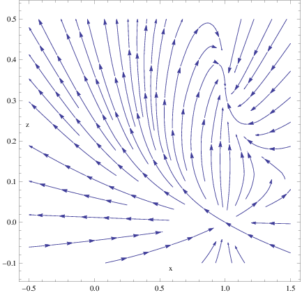
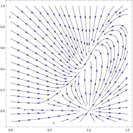
In this case, the stationary points are the following, , and , . For the first fixed point we have and for the second one . The behavior of the trajectories corresponding to this case can be found in Fig. 9, for the choice , , and in Fig. 10, for the choice , .
V Dark Matter Interacting with Dark Energy: Some non-trivial Models
Let us now discuss some non-trivial models which describe interactions between the dark matter and dark energy fluids. The dynamical system in this case may be written in the following form,
| (62) | |||||
| (63) | |||||
| (64) | |||||
| (65) | |||||
| (66) |
where we modified the interaction between dark energy and dark matter by using the multiplier 66 6 Note that case corresponds to the standard interaction we presented in a previous section., and also the term , which corresponds to the bulk viscous pressure of the dark matter fluid. We will assume that the bulk viscous coefficient has the following form,
| (67) |
We define the set of dimensionless variables as follows,
| (68) | |||||
| (69) | |||||
| (70) | |||||
| (71) |
where only and are dynamical independent variables. In the new variables system, Eqs. (62)-(66) take the form77 7 Note that the constraint (62) and the equation for have already been taken into account for this system.:
| (72) | |||||
| (73) | |||||
| (74) |
and using that the EoS has the form we used in the previous section, namely, , , we obtain,
| (75) | |||||
| (76) | |||||
| (77) |
The effective EoS in this case (for arbitrary functions and ) reads,
| (78) |
which in the case that , , becomes,
| (79) |
Now we consider some special cases, and we start with the case . This case corresponds to the usual interaction term. Since the first two equations are identical to (26)-(27), we have the solutions (29), (30), where we need to add .
Also, since the first two equations do not depend on , the first and second eigenvalues will be totally identical to the ones we obtained in section III, and one additional eigenvalue appears for every stationary point, which is,
| (80) |
Also note that the stability or instability of the point with respect to this additional coordinate , implies stability in the past or in the future correspondingly. It mean that a stable with respect to coordinates , point which have will be stable in the past if it is stable with respect to coordinate , or equivalently will be stable for infinite values of . In addition, it will stable in the future, if it is unstable with respect to coordinate , or equivalently it will be stable for small (zero) values of .
The effective EoS (79) for the fixed point (29) is equal to for any values of parameters, which clearly describes a radiation dominated era. However, the effective EoS for the fixed points (30), has a more complicate structure, which is given below,
| (81) |
Let us now further analyze the case at hand, by specifying the values of the free parameters, so we start with the parameter , and assume for the moment that . In this case the fixed point (31) has an additional eigenvalue and the corresponding effective EoS becomes , which describes radiation. Moreover, the fixed point (34) has the additional eigenvalue and the corresponding effective EoS for this point is . Thus in Fig. 1 the left fixed point corresponds to radiation with , and the right point has , and for both the fixed points, has infinite values. In Table 1 we have gathered all the fixed points which correspond to the case , .
| 1a | |||||||
|---|---|---|---|---|---|---|---|
| 1b |
As it can be seen in Table 1, the fixed point may describe late-time acceleration. Indeed, if we set , with , we obtain , and and as we already noted, this means that this point is stable in the future (for small values of ). Moreover, by changing the parameter , we can provide any interesting relation between and . For instance if put we obtain for this point .
Let us discuss some alternative choices for the parameters, so consider the case , in which case the fixed point (37) has an additional eigenvalue, which we denote , and it is equal to, and the corresponding effective EoS is . In addition, the fixed point (38) has the additional eigenvalue with , which describes a matter dominated state. Finally, the fixed point (39) has with . In Table 2 we have gathered all the fixed points for the case .
| 2a | |||||||
| 2b | |||||||
| 2c |
As it can be seen in Table 2, the fixed point is always unstable, if it lies in the physical region, that is, when . The fixed point may be stable in the past and in the future, depending on the values of the parameters. Finally, the fixed point may be stable only if . So in this case, no fixed point describes late-time acceleration, however, the fixed points and may describe a radiation dominated era and matter dominated era respectively.
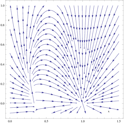
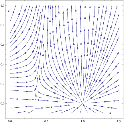
Consider now the case , , in which case, the fixed point (40) has the additional eigenvalue and the corresponding effective EoS is . Accordingly, the fixed point (41) has with and finally the fixed point (42) has with . Thus in Fig.2 we have for the fixed point , for the fixed point and for the fixed point . Correspondingly, in Fig. 3 we have for the fixed point , for the fixed point and for the fixed point . Note that all the aforementioned fixed points correspond to states which have infinite values of .
| 3a | |||||||
|---|---|---|---|---|---|---|---|
| 3b | |||||||
| 3c |
In Table 3 we have gathered all the fixed points for the case , .
Now let us consider some alternative choices for the parameter , and we start with the case , in which case the only stationary point is the following,
| (82) |
and the expression (79) yields for this fixed point,
| (83) |
The effective EoS parameter above describes a de Sitter evolution, with a finite value for the Hubble parameter, namely , which may be arbitrarily small, depending on the values of the other parameters. The eigenvalues for this fixed point in the most general case, have a quite complicate form, but there is one special case for which we can compute these analytically, and this occurs when . In this case, the eigenvalues are,
| (84) | |||||
| (85) |
where the first eigenvalue corresponds to variable . We can see that the stability with respect to all dimensions, requires the following conditions to hold true,
| (87) | |||||
| (88) |
which is quite compatible with , but incompatible with , which reads . This means that by varying the parameters, we can make this point stable with respect to the coordinates and , and unstable with respect , so this point may be used for the construction of the late-time acceleration phase. Note also that by changing value of , it is quite possible to make this point stable with respect to all the coordinates.
Consider now the case , in which case there are four stationary points, which can be found in Table 4. Note that the parameter appearing in Table 4 is equal to . The corresponding eigenvalues can be found in Table 5.
| 4a | ||||
|---|---|---|---|---|
| 4b | ||||
| 4c | ||||
| 4d |
By looking the Table 4 it can be seen that the most phenomenologically interesting fixed point is . First of all it is easy to make this fixed point a stable attractor. Moreover is equal to exactly, so this point corresponds to some de Sitter solution. Finally, for this point we have which means that this point corresponds to some state with non-zero (and non-infinite) value of the Hubble parameter . So by changing the values of the parameters it is easy to make sufficiently large, which implies sufficiently small values of . For instance, by choosing , and we can make this fixed point stable. By assigning sufficiently large values of for sufficiently small (positive) values of , we get large values for . And finally we can see that by changing the values of the parameters, it is easy to construct some fixed relation . In conclusion, this de Sitter attractor may be viewed as a late-time attractor.
| 4a | |||
|---|---|---|---|
| 4b | |||
| 4c | |||
| 4d |
It is interesting to note that there are five different regions in the parameter space, for which all four stationary points lie in the physical region, and these regions are the following,88 8 i.e. , , for all points simultaneously.
| (89) | |||
| (90) | |||
| (91) | |||
| (92) | |||
| (93) |
where
However, the above cases are quite hard to be tackled analytically, so a numerical study is needed, which exceeds the purposes of this article.
V.1 Oscillating Dark Energy-Dark Matter Interaction
In the previous sections we considered cases of dark energy and dark matter interactions, by specifying the free parameters, and in this section we follow a different approach: we will directly modify the functional form of the dark energy-dark matter interaction by making it oscillating. So assume that in Eq. (65) we make the following replacement, . In effect, instead of Eqs. (75)-(77) we have
| (94) | |||||
| (95) | |||||
| (96) |
where . Let us suppose that the argument of the cosine function changes monotonically, from during the inflationary era, when , to which corresponds at the present time. In practice we may realize this kind of behavior by assuming sufficiently small values of the parameter . Then, the physical interpretation of the situation at hand is the following, at early times (inflationary era), there is no interaction between the various matter fluid components, and as the time grows, this interaction starts to develop, and it grows until it reaches its maximum value at . From a mathematical point of view, this would mean that there are two distinct asymptotic states at and , which are described by two distinct dynamical systems. In the following we discuss these two asymptotic dynamical systems separately.
V.1.1 Asymptotic State I: The Inflationary Epoch
Let us now focus on the inflationary asymptotic state, in which case instead of (94)-(96), we have the following dynamical system,
| (97) | |||||
| (98) | |||||
| (99) |
where for the stationary points in the last equation above, we must put . We can see that the last equation is decoupled from the system, and mainly governs the stability with respect to the variable only. The stationary points of the system (97)-(98) are already found in section III and these are presented in Eqs. (29)-(30), where we need to put . The first fixed point should be excluded from the future investigation, since it has . Thus we have one possible fixed point candidate that may describe inflation (let us denote it ):
| (100) |
with,
| (101) |
Now in order to describe inflation, we need to construct a de Sitter solution, which should be stable with respect to the coordinates , and unstable with respect to , in order to provide an exit from inflation. Thus let us put for (101) , where . In this case, the third eigenvalue associated with the coordinate will exactly be , so this provides an instability of de Sitter point. Moreover deriving from (101) and equating it to (100), we find an additional relation between the free parameters,
| (102) |
or if we require that all the values of parameters are not very small in comparison with , we have,
| (103) |
V.1.2 Asymptotic State II: Present Time and Late-time Acceleration
Now let us consider the present-time asymptotic case, in which case instead of the dynamical system of Eqs. (94)-(96) we have the following system,
| (104) | |||||
| (105) | |||||
| (106) |
where for stationary points in the last equation we must require . Thus, from the last equation we have
| (107) |
Substituting the above in Eq. (104) we find,
and by substituting in Eq. (105) we find,
In effect, the system will compatible only if the following condition holds true,
which gives us,
| (108) |
and the corresponding stationary point is (let us denote it )
| (109) |
Combining (108) with (103) we find,
| (110) |
so we can see that is very small but does not vanish.99 9 Putting exactly for the first point, we get . Note also that the effective EoS for this point, calculated for (79) yields exactly for any values of the parameters.
V.1.3 combining and stability analysis.
By looking the differential equations in Eqs. (97)-(98) and (104)-(105), it can be seen that these are identical apart for some additive constants, and in effect the eigenvalues will be identical for the two systems. Let us denote and for notational simplicity. In effect, the equation that determines the eigenvalues, takes the following form,
| (111) |
where , , and , are equal to,
and in the above relations we took into account that for both points we have .
The solution of Eq. (111) for the fixed point with positive sign in (100) reads,
| (112) |
and for the point
| (113) |
and by substituting the expression (103) for , for the fixed point , we have,
| (114) |
and for the point we get,
| (115) |
Note that we have set , since all the eigenvalues, even in this case, do not vanish. Thus we can see that both points and are stable or unstable with respect to coordinates and simultaneously, and stability condition reads,
| (116) |
Moreover, we need to require that both fixed points lie in the physical region, namely at and , so the following conditions must be satisfied,
| (117) | |||
| (118) | |||
| (119) | |||
| (120) |
where,
In Table 6 we have gathered all the fixed points and the corresponding eigenvalues for the case of an oscillating form of the interaction term .
| 5a | ||||||
|---|---|---|---|---|---|---|
| 5b |
It is worth discussing some interesting scenarios, so assume that , , then the fixed points and the eigenvalues become,
So by changing the values of the parameters and , it is possible to appropriately fix the fixed point , which recall that it corresponds to late-time acceleration, in order some fixed relation between and holds true. Note that in this section we studied only case for which the choices of the functions and were the simplest choices, but in principle a more involved functional form for these functions may lead to more interesting phenomenology. In such a case though, the analytical treatment will be possibly insufficient, so a concrete numerical analysis will be needed.
In conclusion, we constructed a cosmological model that describes the inflationary and the late-time acceleration era, due to an oscillating interaction term between the dark energy and dark matter fluids. We found two fixed points, with the first being , which describes the initial de Sitter solution, namely the inflationary era, and this fixed point was unstable, a feature which indicates that the graceful exit is triggered. The second fixed point was also found to be a de Sitter fixed point, which describes the present day acceleration. As we demonstrated, in the oscillating model we discussed, during the early Universe there was no interaction between dark energy and dark matter, however during the late-time the interaction was present. Finally, as we showed, by appropriately choosing the parameters, it is possible to produce some fixed relation for .
Before closing this section, let us briefly discuss an interesting issue with regards the early-time era. It would be interesting to calculate the slow-roll indices and the corresponding observational indices for the inflationary era we presented in section V.1.1. For example by assuming the perfect fluid approach [7], we can express the spectral index of primordial curvature perturbations and the scalar-to-tensor ratio in the usual way these are given in the case of a canonical scalar field,
with the slow-roll indices being defined in terms of the Hubble rate as follows,
By combining Eqs. (62) and (63) it is easy to calculate the slow-roll parameter , which reads,
Differentiating (63) and by combining with equations (62)-(66) we can find a similar expression for the slow-roll parameter . Note here that the resulting expression for is much more complicated so we omit it. There is a major obstacle in calculating the slow-roll indices however, since in the expressions for and , we must use values for and not on the stationary point, but from some point near the stationary point. The resulting slow-roll indices must be expressed in terms of the -foldings number , but doing this analytically is a rather formidable task, that exceeds the purposes of this work. A numerical approach though might be less difficult to perform, so we hope to address this task in a future work.
VI Conclusions
In this work we analyzed in detail the phase space of a cosmological system that contains cosmological fluids that have various forms of equation of state. We firstly discussed the simplest forms of EoS, and we found the fixed points of the cosmological dynamical system and we discussed the physical significance of these fixed points. In addition, we discussed theories that admit interactions between the dark energy and dark matter fluids. In addition we introduced a new class of interaction between dark energy and dark matter, in which theories the interaction term is oscillating, allowing different form of interactions for various eras during the cosmological evolution. As we demonstrated, it is possible to have almost negligible interactions at early times, that is, during the inflationary era, and for the same model the interaction is turned on at late times. The cosmological dynamical system of the oscillating interaction term is in turn decomposed into two distinct dynamical systems at early and late times. Interestingly enough the two dynamical systems predict two de Sitter fixed points corresponding to early and late times, with the early-time de Sitter point being unstable in one of the coordinates, a feature which indicates the possible exit from the inflationary era. This framework gives us the interesting fluid-filled Universe evolution, unifying the early-time acceleration with late-time acceleration.
The fluid description offers an alternative viewpoint in modern cosmology, which may describe successfully many eras of our Universe’s evolution. The dynamical system approach offers many new insights since the fixed points of the dynamical system reveal the attractors of the whole theory and their stability indicates whether these attractors are final attractors of the system. A compelling extension of this work is to include Loop Quantum Cosmology effects in the EoS, as was performed in Ref. [14], so we defer this task to a future work. Another strong motivation to adopt the fluid approach in cosmology, is the late-time acceleration era, since this can be modeled by fluid cosmology [59]. Furthermore, as modified gravity maybe easily presented in the effective fluid representation, the dynamical systems approach turns out to be useful also for the study of the cosmology in modified gravity. More interestingly, the dynamical system approach can be applied to the study of bouncing cosmology, described by a multi-component fluid. We aim to address this latter issue in a future work. In conclusion, we believe that the multi-component fluid cosmology may have some valuable insights to offer to the cosmologists community.
Acknowledgements.
This work was supported by the Russian Science Foundation (RSF) grant 16-12-10401 (P.V.T.), by the Russian Foundation for Basic Research (RFBR) grant 17-02-01008 À (P.V.T.), by MINECO (Spain), project FIS2013-44881, FIS2016-76363-P and by CSIC I-LINK1019 Project (S.D.O) and by the Russian Ministry of Education and Science, Project No. 3.1386.2017 (S.D.O and V.K.O).References
- [1] A.G. Riess et al. (High-z Supernova Search Team), Astronom. J. 116, 1009 (1998) [arXiv:astro-ph/9805201]
- [2] S. Nojiri, S. D. Odintsov and V. K. Oikonomou, arXiv:1705.11098 [gr-qc].
- [3] S. Nojiri and S. D. Odintsov, Phys. Rept. 505 (2011) 59 doi:10.1016/j.physrep.2011.04.001 [arXiv:1011.0544 [gr-qc]]
- [4] S. Nojiri and S. D. Odintsov, eConf C 0602061 (2006) 06 [Int. J. Geom. Meth. Mod. Phys. 4 (2007) 115] doi:10.1142/S0219887807001928 [hep-th/0601213].
- [5] V. Faraoni and S. Capozziello, Fundam. Theor. Phys. 170 (2010). doi:10.1007/978-94-007-0165-6
- [6] S. Nojiri and S. D. Odintsov, Phys. Rev. D 72 (2005) 023003 [hep-th/0505215]
- [7] K. Bamba, S. Nojiri, S. D. Odintsov and D. Sáez-Gómez, Phys. Rev. D 90 (2014) 124061 [arXiv:1410.3993 [hep-th]].
- [8] S. Capozziello, V. F. Cardone, E. Elizalde, S. Nojiri and S. D. Odintsov, Phys. Rev. D 73 (2006) 043512 [astro-ph/0508350].
- [9] I. Brevik and Ø. Grøn, arXiv:1409.8561 [gr-qc].
- [10] M. Szydlowski, W. Godlowski and R. Wojtak, Gen. Rel. Grav. 38 (2006) 795 [astro-ph/0505202].
- [11] X. Chen, H. Firouzjahi, M. H. Namjoo and M. Sasaki, JCAP 1309 (2013) 012 [arXiv:1306.2901 [hep-th]]
- [12] R. Myrzakulov and L. Sebastiani, Astrophys. Space Sci. 356 (2015) 1, 205 [arXiv:1410.3573 [gr-qc]]
- [13] I. Brevik, O. Gron, J. de Haro, S. D. Odintsov and E. N. Saridakis, arXiv:1706.02543 [gr-qc].
- [14] V. K. Oikonomou, arXiv:1703.09009 [gr-qc].
- [15] S. Nojiri, S. D. Odintsov and V. K. Oikonomou, Phys. Lett. B 747 (2015) 310 [arXiv:1506.03307 [gr-qc]].
- [16] I. Brevik and A. V. Timoshkin, Int. J. Geom. Meth. Mod. Phys. 14 (2017) no.04, 1750061 [arXiv:1612.06689 [gr-qc]].
- [17] A. Avelino, Y. Leyva and L. A. Urena-Lopez, Phys. Rev. D 88, 123004 (2013).
- [18] N. Cruz, S. Lepe, Y. Leyva, F. Pena and J. Saavedra, Phys. Rev. D 90, 083524 (2014).
- [19] Y. Leyva and M. Sepulveda, arXiv:1611.03833 [gr-qc].
- [20] H. Velten, J. Wang and X. Meng, Phys. Rev. D 88, 123504 (2013).
- [21] H. Velten and D. Schwarz, Phys. Rev. D 86, 083501 (2012).
- [22] H. Velten, T. R. P. Carames, J. C. Fabris, L. Casarini and R. C. Batista, Phys. Rev. D 90, 123526 (2014).
- [23] H. Velten, D. J. Schwarz, J. C. Fabris and W. Zimdahl, Phys. Rev. D 88, 103522 (2013).
- [24] H. Velten, Int. J. Geom. Meth. Mod. Phys. 11, 1460013 (2014).
- [25] W. Israel and J. M. Stewart, Annals Phys. 118, 341 (1979).
- [26] R. Maartens, astro-ph/9609119.
- [27] N. Cruz, S. Lepe and F. Pena, Phys. Lett. B 767, 103 (2017).
- [28] M. Cruz, N. Cruz and S. Lepe, Phys. Lett. B 769, 159 (2017).
- [29] S. Lepe, G. Otalora, J. Saavedra , arXiv:1704.05625 [gr-qc].
- [30] W. Zimdahl and D. Pavon, Phys. Lett. B 521, 133 (2001).
- [31] G. Caldera-Cabral, R. Maartens and L. A. Urena-Lopez, Phys. Rev. D 79, 063518 (2009); AIP Conf. Proc. 1241, 741 (2010).
- [32]
A. A. Coley,
gr-qc/9910074.;
G. Leon and C. R. Fadragas, arXiv:1412.5701 [gr-qc]. - [33] R. Garcia-Salcedo, T. Gonzalez and I. Quiros, arXiv:1211.2738 [gr-qc].
- [34] C. G. Boehmer, G. Caldera-Cabral, R. Lazkoz and R. Maartens, Phys. Rev. D 78 (2008) 023505 doi:10.1103/PhysRevD.78.023505 [arXiv:0801.1565 [gr-qc]].
- [35] C. G. Boehmer and N. Chan, arXiv:1409.5585 [gr-qc].
- [36] Z. Haba, A. Stachowski and M. Szydlowski, JCAP 1607 (2016) no.07, 024 doi:10.1088/1475-7516/2016/07/024 [arXiv:1603.07620 [gr-qc]].
- [37] Y. L. Bolotin, A. Kostenko, O. A. Lemets and D. A. Yerokhin, Int. J. Mod. Phys. D 24 (2014) no.03, 1530007 doi:10.1142/S0218271815300074 [arXiv:1310.0085 [astro-ph.CO]].
- [38] M. Abdelwahab, S. Carloni and P. K. S. Dunsby, Class. Quant. Grav. 25 (2008) 135002 doi:10.1088/0264-9381/25/13/135002 [arXiv:0706.1375 [gr-qc]].
- [39] S. Carloni, S. Capozziello, J. A. Leach and P. K. S. Dunsby, Class. Quant. Grav. 25 (2008) 035008 doi:10.1088/0264-9381/25/3/035008 [gr-qc/0701009].
- [40] S. Carloni, P. K. S. Dunsby, S. Capozziello and A. Troisi, Class. Quant. Grav. 22 (2005) 4839 doi:10.1088/0264-9381/22/22/011 [gr-qc/0410046].
- [41] G. Leon and E. N. Saridakis, JCAP 1504 (2015) no.04, 031 doi:10.1088/1475-7516/2015/04/031 [arXiv:1501.00488 [gr-qc]].
- [42] C. Xu, E. N. Saridakis and G. Leon, JCAP 1207 (2012) 005 doi:10.1088/1475-7516/2012/07/005 [arXiv:1202.3781 [gr-qc]].
- [43] S. Carloni and J. P. Mimoso, arXiv:1701.00231 [gr-qc].
- [44] G. Leon and E. N. Saridakis, Class. Quant. Grav. 28 (2011) 065008 doi:10.1088/0264-9381/28/6/065008 [arXiv:1007.3956 [gr-qc]].
- [45] S. Carloni, A. Troisi and P. K. S. Dunsby, Gen. Rel. Grav. 41 (2009) 1757 doi:10.1007/s10714-008-0747-9 [arXiv:0706.0452 [gr-qc]].
- [46] M. Khurshudyan, Int. J. Geom. Meth. Mod. Phys. 14 (2016) no.03, 1750041. doi:10.1142/S0219887817500414
- [47] M. Hohmann, L. Jarv and U. Ualikhanova, arXiv:1706.02376 [gr-qc].
- [48] S. D. Odintsov and V. K. Oikonomou, Phys. Rev. D 93 (2016) no.2, 023517 doi:10.1103/PhysRevD.93.023517 [arXiv:1511.04559 [gr-qc]].
- [49] M. Skugoreva, A. Toporensky and P. Tretyakov, Grav. Cosmol. 17 (2011) 110 [arXiv:1007.3365 [gr-qc]].
- [50] S. Nojiri and S. D. Odintsov, Phys. Rev. D 72 (2005) 023003 doi:10.1103/PhysRevD.72.023003 [hep-th/0505215].
- [51] K. Bamba, S. Capozziello, S. Nojiri and S. D. Odintsov, Astrophys. Space Sci. 342 (2012) 155 doi:10.1007/s10509-012-1181-8 [arXiv:1205.3421 [gr-qc]].
- [52] C. W. Misner, Astrophys. J. 151 (1968) 431. doi:10.1086/149448
- [53] K. Bamba, Int. J. Geom. Meth. Mod. Phys. 13 (2016) no.06, 1630007 [arXiv:1604.02632 [gr-qc]].
- [54] I. H. Brevik and O. Gorbunova, Gen. Rel. Grav. 37 (2005) 2039 doi:10.1007/s10714-005-0178-9 [gr-qc/0504001].
- [55] I. H. Brevik, E. Elizalde, O. Gorbunova and A. V. Timoshkin, Eur. Phys. J. C 52 (2007) 223 doi:10.1140/epjc/s10052-007-0357-9 [arXiv:0706.2072 [gr-qc]].
- [56] B. D. Normann and I. Brevik, Entropy, Vol. 18, article 215 (2016) doi:10.3390/e18060215 [arXiv:1601.04519 [gr-qc]].
- [57] J. D. Barrow and S. Hervik, Phys. Rev. D 74 (2006) 124017 doi:10.1103/PhysRevD.74.124017 [gr-qc/0610013].
- [58] V. K. Oikonomou and N. Karagiannakis, Class. Quant. Grav. 32 (2015) no.8, 085001 doi:10.1088/0264-9381/32/8/085001 [arXiv:1408.5353 [gr-qc]].
- [59]
A. B. Balakin and V. V. Bochkarev,
Phys. Rev. D 83 (2011) 024036
doi:10.1103/PhysRevD.83.024036
[arXiv:1012.2433 [gr-qc]].;
N. Cruz, S. Lepe and F. Pena, Phys. Lett. B 663 (2008) 338 doi:10.1016/j.physletb.2008.04.035 [arXiv:0804.3777 [hep-ph]].