The 2D Tree Sliding Window Discrete Fourier TransformThanks: Authors’ addresses: Department of Statistics and Data Science, Carnegie Mellon University, 5000 Forbes Ave, Pittsburgh, PA 15213

The 1D SWDFT takes a sequence of DFTs within each position of a sliding window. Specifically, let ${\bf x}=[x_{0},x_{1},\ldots,x_{N-1}]$ be a length $N$ complex-valued signal, and let $n\leq N$ be the window size. Indexing the window position by $p=n-1,n,\ldots N-1$, the 1D SWDFT is:

for $k=0,1,\ldots N-1$, where $\omega_{n}=\exp{\frac{i2\pi}{n}}=\cos{\frac{2\pi}{N}}+i\sin{\frac{2\pi}{N}}$.

A straightforward calculation of Equation 1 takes $Pn^{2}$ operations, where $P=N-n+1$ is the number of window positions. Replacing the DFT with an FFT for each window position reduces this to $O(Pn\log{n})$ operations. The fast algorithm described in this section, in addition to the algorithms described in Section 2, further reduces the computational complexity to $O(Pn)$.

We clarify a few points regarding the FFT algorithm used in this paper. First, while many different FFT algorithms have been developed (e.g. (Rabiner et al., 1969; Good, 1958)), we focus on the (Cooley and Tukey, 1965) algorithm. So whenever we say FFT, we are referring to the Cooley-Tukey algorithm. Next, since the FFT factorizes a length $n$ signal, different algorithms exist for different $n$. This paper only considers in detail when $n$ is a power of two, called the Radix-2 case. However, the Cooley-Tukey algorithm easily extends to arbitrary factorizations.

The 1D Tree SWDFT algorithm takes a 1D FFT in each window, and avoids repeating calculations already computed in previous windows by storing them in a tree data-structure. Understanding which calculations have already been computed requires a detailed understanding of the FFT. Figure 1 shows the famous butterfly diagram, giving FFT calculations for a length $n=8$ signal. The squares on the left of Figure 1 correspond to the input data, the circles on the right are the output DFT coefficients, and the arrows in the middle are the calculations. Both (Covell and Richardson, 1991) and (Farhang and Lim, 1992) derived their non-recursive algorithms by showing that calculations in the butterfly diagram repeat in overlapping windows.

An equivalent tree diagram of the FFT is shown in the top panel of Figure 2. It is important to stress that the calculations in the butterfly and tree diagrams are the same. For sliding windows, the tree diagram has two major advantages. First, the input data and output coefficients are ordered. Second, underneath $x_{7}$ is a binary tree with three (since $2^{3}=8$) levels, and the final level of this binary tree contains the DFT coefficients.

Figure 2 demonstrates the 1D Tree SWDFT algorithm. The top panel shows calculations for the window position one with input data $[x_{0},x_{1},\ldots,x_{7}]$, and the bottom panel shows the calculations for window position two with input data $[x_{1},x_{2},\ldots,x_{8}]$. In window two, solid arrows represent computations made in window one, and dashed arrows represent new window two calculations. The number of new window two calculations is exactly the size of the binary tree, and the difference between the number of solid and dashed arrows is exactly the log factor speed up gained by the 1D Tree SWDFT algorithm.

Implementing the 1D Tree SWDFT requires calculating each node of each binary tree, which corresponds to three nested loops:

1. (1)

   over $N$ trees

2. (2)

   over $\log_{2}(n)$ levels

3. (3)

   over $2^{l}$ nodes at level $l$ of each tree.

The only restriction on loop order is that loop 2 (over levels) must precede loop 3 (over nodes), since nodes at lower levels of the tree depend on nodes at higher levels. There are three possible loop orders: ($1,2,3$), ($2,1,3$), and ($2,3,1$); the first ordering would be appropriate for data which arrives sequentially in time.

The 2D SWDFT of an $N_{0}\times N_{1}$ array calculates a 2D DFT for all $n_{0}\times n_{1}$ windows. This derivation requires that $n_{0}=2^{m_{0}}$ and $n_{1}=2^{m_{1}}$, the Radix-2 case. Let x be an $N_{0}\times N_{1}$ array. There are $P_{i}=N_{i}-n_{i}+1;i=0,1$ window positions in each direction, making $P_{0}P_{1}$ total window positions. Indexing the window position by $(p_{0},p_{1})$, where $p_{i}=n_{i}-1,n_{i},\ldots,N_{i}-1;i=0,1$, the 2D SWDFT is:

where $k_{i}=0,1,\ldots,n_{i}-1;i=0,1$. Equation 2 outputs a $P_{0}\times P_{1}\times n_{0}\times n_{1}$ array.

A straightforward calculation of Equation 2 takes $P_{0}P_{1}n_{0}^{2}n_{1}^{2}$ operations. Replacing the 2D DFT with a 2D FFT (described next) reduces the number of operations to $O(P_{1}P_{0}n_{0}n_{1}\log(n_{0}n_{1}))$. Our algorithm, along with the algorithms of (Park, 2015a) and (Byun et al., 2016), further reduce this to $O(P_{0}P_{1}n_{0}n_{1})$.

Conceptually, the 2D Tree SWDFT algorithm works like 1D. As in 1D, there is a tree data-structure with 2D FFT calculations underneath each data-point (see top panel of Figure 3). Also like 1D, the 2D Tree SWDFT reuses 2D FFT calculations computed in previous windows. Finally, just like there are different 1D FFT algorithms, there are also different 2D FFT algorithms (see Section 9 of (Duhamel and Vetterli, 1990)).

Since the 2D Tree SWDFT computes a 2D FFT for each window position, and different 2D FFT algorithms exist, our 2D Tree SWDFT derivation requires specifying which 2D FFT to use. The two most commonly used 2D FFTs are the Row-Column FFT and the Vector-Radix FFT. This derivation uses the Row-Column FFT due to its flexibility and straightforward implementation. However, the 2D Tree SWDFT can also be derived by swapping the Row-Column FFT with the Vector-Radix FFT ((Byun et al., 2016)). To be clear, the 2D Tree SWDFT algorithm takes a 2D FFT in each window position, and stores the intermediate calculations in a tree data-structure. The Row-Column FFT is the specific 2D FFT algorithm used in this derivation of the 2D Tree SWDFT algorithm.

The key to the Row-Column FFT is the “factorization” property of the 2D DFT. Factorization means that 2D DFTs can be computed using 1D DFTs:

This implies the 2D DFT can be computed by first taking 1D FFTs of each row ($z_{j_{0},k_{1}}$), followed by 1D FFTs of the resulting columns. This sequence of 1D FFTs is exactly the Row-Column FFT.

Though conceptually similar, several details differentiate the 1D and 2D Tree SWDFT algorithms. In 2D, the trees underneath each data-point are two-dimensional, where the two dimensions are $m_{0}=\log_{2}(n_{0})$ and $m_{1}=\log_{2}(n_{1})$. Second, we now require two twiddle-factor vectors; Twiddle factors (named by (Gentleman and Sande, 1966)) are the trigonometric constants used for combining smaller DFTs during the FFT algorithm (the $\omega$’s in Figures 1 and 2 are twiddle factors). Finally, when the window slides by one position, we now replace an entire row or column, as opposed to a single data-point in 1D.

Figure 3 shows how the 2D Tree SWDFT works. The solid arrows in window two indicate 2D FFT calculations from window one, and the dashed arrows are the new calculations required for window two. Like 1D, the number of dashed lines is exactly the size of the tree underneath the bottom-right point $(x_{1,4})$ of window two. With this preamble, we are ready to derive the 2D Tree SWDFT.

Let x be a $N_{0}\times N_{1}$ array, with window sizes $n_{0}\times n_{1}$, where $n_{0}=2^{m_{0}}$ and $n_{1}=2^{m_{1}}$, the Radix-2 case. We do not require that $n_{0}=n_{1}$. Our trees have $m_{0}+m_{1}$ levels: the first $m_{0}$ levels correspond to 1D row FFTs, the next $m_{1}$ levels correspond to 1D column FFTs, and the final level $(m_{0}+m_{1})$ is the 2D DFT coefficients. Let $\Omega^{i}=[\omega_{n_{i}}^{0},\omega_{n_{i}}^{-1},\ldots,\omega_{n_{i}}^{-(n_{i}-1)}];i=0,1$ be a length $n_{i}$ twiddle-factor vector. Finally, let T be the tree data-structure that stores 2D FFT calculations for each window position. We access T by window position, level, and node. For example, $T_{p_{0},p_{1},l,i_{0},i_{1}}$ corresponds to node $(i_{0},i_{1})$ on the $l^{th}$ level of the tree at window position $(p_{0},p_{1})$.

We give the calculations for an arbitrary tree at window position $(p_{0},p_{1})$. Each level $l$ has $2^{l}$ nodes. Level zero of the tree is the data: $T_{p_{0},p_{1},0,0,0}=x_{p_{0},p_{1}}$. We use one additional piece of notation: let $s_{l}^{d}$ be the “shift” for dimension $d$ and level $l$. The “shift” ($s_{l}^{d}$) identifies which tree has the repeated calculation needed for the current calculation. For example, if $s_{1}^{0}=2$, this means for level 1, the repeated calculation is located at tree $(p_{0}-2,p_{1})$. For levels corresponding to row FFTs: $s_{l}^{1}=2^{m_{1}-l}$, and for column FFT levels: $s_{l}^{0}=2^{m_{0}+m_{1}-l}$.

Level one of tree $(p_{0},p_{1})$ has $2^{1}=2$ nodes: $(0,0),(0,1)$. The shift is $s_{1}^{1}=2^{m_{1}-1}$, meaning the repeated calculation is at tree $(p_{0},p_{1}-s_{1}^{1})$. For node $(0,i_{1})$, the calculation is a complex multiplication between node $(0,i_{1}\text{ mod }2^{1-1})=(0,0)$ at level $1-1=0$ of the current tree $(p_{0},p_{1})$, and the $i_{1}\cdot s_{1}^{1}$ element from twiddle-factor vector $\Omega^{1}$. The complex multiplication output is then added to node $(0,0)$ from the shifted tree $(p_{0},p_{1}-s_{1}^{1})$. Using our tree notation:

for $i_{1}=0,1$, which is a length two DFT of $x_{p_{0},p_{1}}$ and $x_{p_{0},p_{1}-s_{1}^{1}}$.

Calculating each node of T has the same form: $T_{A}=T_{B}+\Omega^{i}_{C}\cdot T_{D}$. $A,B,C$ and $D$ are indices into either T, $\Omega^{0}$, or $\Omega^{1}$, depending on whether the level $l$ of the tree corresponds to the row ($1$ to $m_{1}$) or column ($m_{1}+1$ to $m_{1}+m_{0}$) part of the Row-Column FFT. We give the exact calculations for both situations next.

Level $t\leq m_{1}$ of tree $(p_{0},p_{1})$ has $2^{t}$ nodes: 1 in the row-direction, and $2^{t}$ in the column-direction. The repeated calculation comes from tree $(p_{0},p_{1}-s_{t}^{1})$, where $s_{t}^{1}=2^{m_{1}-t}$. For node $(0,i_{1});i_{1}=0,1,\ldots 2^{t}-1$, the calculation is:

Level $v>m_{1}$ of tree $(p_{0},p_{1})$ has $2^{v}$ nodes: $2^{v-m_{1}}$ in the row-direction, and $n_{1}$ in the column-direction. The repeated calculation comes from tree $(p_{0}-s_{v}^{0},p_{1})$, where $s_{v}^{0}=2^{m_{0}+m_{1}-l}$. For node $(i_{0},i_{1});i_{0}=0,1,\ldots n_{1},i_{1}=0,1,\ldots 2^{v-m_{1}}-1$, the calculation is:

The final level $(m_{0}+m_{1})$ contains the 2D DFT coefficients for window position $(p_{0},p_{1})$. After calculating T, all that remains is selecting the subset at level $m_{0}+m_{1}$ of each tree, and the algorithm is complete.

After creating the twiddle-factor vectors and allocating memory, we implement the 2D Tree SWDFT in six nested loops:

1. (1)

   over $m_{0}=\log_{2}(n_{0})$ levels corresponding to row FFTs

2. (2)

   over $m_{1}=\log_{2}(n_{1})$ levels corresponding to column FFTs

3. (3)

   over $N_{0}$ trees in the row-direction

4. (4)

   over $N_{1}$ trees in the column-direction

5. (5)

   over $2^{l_{0}}$ nodes in the row-direction at level $l_{0}$

6. (6)

   over $2^{l_{1}}$ nodes in the column-direction at level $l_{1}$

Inside the six loops is either Equation 5 or 6, depending on whether the level corresponds to the row or column part of the Row-Column FFT algorithm.

Since the next level of the trees only depends on the previous level, our implementation allocates $2N_{0}N_{1}n_{0}n_{1}$ complex numbers in memory: $N_{0}N_{0}n_{0}n_{1}$ for both the previous and current level. This is possible because the two loops over levels are innermost. This also implies our algorithm is suitable for parallel computing, following (Wang and Eddy, 2012).

Like 1D, we can swap the order of the loops. For our derivation, the only restrictions are that loop $1$ must precede loop $2$, and loops $5$ and $6$ must come after loops $1$ and $2$. A particularly interesting order is when loops $3$ and $4$ (over trees) are innermost. This version can be tailored to a real-time task, opposed to the “levels innermost” order, which requires all data to be available. For example, if the channels of a multi-spectral scanner are considered as a two-dimensional array, and T is stored, we could calculate the output for a new window in $O(n_{0}n_{1})$ time.

The 2D SWDFT is memory intensive, since the output is a $P_{0}\times P_{1}\times n_{0}\times n_{1}$ array. For example, if $P_{0}=P_{1}=400$, and $n_{0}=n_{1}=32$, then the output is $163,840,000$ complex numbers. Because our implementation uses $16$ byte double complex numbers, the output alone requires $16\cdot 163840000=2621440000$ bytes, or $\approx 2.6$ gigabytes.

Our algorithm extends directly to $k$D. For instance, if we had an $N_{0}\times N_{1}\times\ldots\times N_{k-1}$ array, with $n_{i}=2^{m_{i}}\leq N_{i};i=0,\ldots,k-1$ windows, then the calculation for node $(i_{0},i_{1},\ldots,i_{k-1})$, level $l$, and dimension $c$ is:

where $s_{l}^{c}=2^{(\sum_{i=c}^{k-1}m_{i})-l}$, and dimension $c$ contains levels $[\sum_{i=c+1}^{k-1}m_{i}+1,\sum_{i=c}^{k-1}m_{i}]$ of the trees. Extending the implementation to any dimension is possible following Equation 7. For example, the $3$D implementation takes $9$ loops: $3$ over dimension, $3$ over trees, and $3$ over nodes. The computation inside the loops is one of:

Depending on if level $l$ of the tree is between $[1,m_{2}]$, $[m_{2}+1,m_{2}+m_{1}]$, or $[m_{2}+m_{1}+1,m_{2}+m_{1}+m_{0}]$, respectively. The $4$D implementation follows the same idea with $3\cdot 4=12$ loops, and so on.

In the software package accompanying this paper, our primary contribution is a C implementation of the 2D Tree SWDFT algorithm. The purpose of our implementation is not a specially optimized program, but rather a precise description of how the algorithm works.

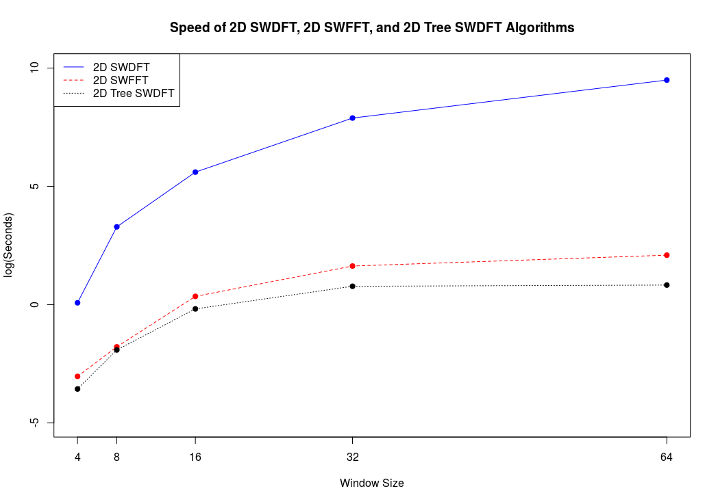
Our package is small and light-weight, and only requires a gcc compiler and C standard libraries to run. The only function included in our primary source code is the 2D Tree SWDFT implementation. We include two other functions to verify the accuracy and stability of our implementation: the 2D SWDFT and 2D SWFFT. The 2D SWDFT takes a 2D DFT in each window position, and the 2D SWFFT takes a 2D FFT in each window position. We include these two functions because other algorithms of comparable theoretical speed ((Park, 2015a; Byun et al., 2016)), to our knowledge, do not have publicly available software implementations. Figure 4 compares the speed of our 2D SWDFT, 2D SWFFT, and 2D Tree SWDFT implementations.

The initial motivation for non-recursive SWDFT algorithms was numerical stability. As discussed in Section 2, recursive algorithms were proposed before non-recursive algorithms, but were quickly identified as numerically unstable. The reason recursive algorithms are numerically unstable is that the complex exponentials (e.g. $\omega_{n}$) are represented with finite precision, and the rounding errors accumulate as the number of window positions increases. In contrast, non-recursive algorithms use the same underlying calculations as FFT algorithms, so the output is identical to the 2D SWFFT. Another way to say this is that the the number of operations for non-recursive algorithms is bounded. For example, computing each coefficient with the 2D Tree SWDFT algorithm takes exactly $2(n_{0}n_{1}-1)$ operations (see Equation 8 below). We include a program in the tests of our software package that shows our algorithm gives identical results to the 2D SWFFT, since both algorithms use identical intermediate calculations.

The run-time of the 2D Tree SWDFT algorithm grows linearly in window ($n_{0}n_{1}$) and array ($N_{0}N_{1}$) size. This is because calculating each node requires one complex multiplication and one complex addition, defined as an operation (the same definition was used in (Cooley and Tukey, 1965)). Since level $l$ requires $2^{l}$ operations, number of operations per window is:

The exact run-time is slightly more complicated, since windows with indices either less than $n_{0}$ in the row direction or less than $n_{1}$ in the column direction do not require complete trees. These extra calculations are negligible for large arrays, so the 2D Tree SWDFT takes $O(P_{0}P_{1}n_{0}n_{1})$ operations. Table 1 compares the speed, memory, and properties of the 2D Tree SWDFT with existing algorithms. Our memory numbers for (Park, 2015a) and (Byun et al., 2016) come from the Table 2 in (Byun et al., 2016). Out of existing $O(P_{0}P_{1}n_{0}n_{1})$ algorithms, our 2D Tree SWDFT is the only one that is numerically stable, works for non-square windows, and has an existing publicly available software implementation.

References

- Albrecht and Cumming (1999) Sandor Albrecht and Ian Cumming. 1999. Application of momentary Fourier transform to SAR processing. IEE Proceedings-Radar, Sonar and Navigation 146, 6 (1999), 285–297.
- Albrecht et al. (1997) S Albrecht, I Cumming, and J Dudas. 1997. The momentary Fourier transformation derived from recursive matrix transformations. In Digital Signal Processing Proceedings, 1997. DSP 97., 1997 13th International Conference on, Vol. 1. IEEE, 337–340.
- Amin (1987) Moeness G Amin. 1987. A new approach to recursive Fourier transform. Proc. IEEE 75, 11 (1987), 1537–1538.
- Aravena (1990) Jorge L. Aravena. 1990. Recursive moving window DFT algorithm. IEEE Trans. Comput. 39, 1 (1990), 145–148.
- Bitmead (1982) R Bitmead. 1982. On recursive discrete Fourier transformation. IEEE Transactions on Acoustics, Speech, and Signal Processing 30, 2 (1982), 319–322.
- Bongiovanni et al. (1975) G Bongiovanni, P Corsini, and G Frosini. 1975. Non-recursive real time Fourier analysis. Consiglio Nazionale delle Ricerche. Istituto di Elaborazione della Informazione Pisa.
- Bongiovanni et al. (1976) Giancarlo Bongiovanni, Paolo Corsini, and Graziano Frosini. 1976. Procedures for computing the discrete Fourier transform on staggered blocks. IEEE Transactions on Acoustics, Speech, and Signal Processing 24, 2 (1976), 132–137.
- Bracewell (1986) Ronald Newbold Bracewell. 1986. The Fourier transform and its applications. Vol. 31999. McGraw-Hill New York.
- Byun et al. (2016) Keun-Yung Byun, Chun-Su Park, Jee-Young Sun, and Sung-Jea Ko. 2016. Vector Radix 2 2 Sliding Fast Fourier Transform. Mathematical Problems in Engineering 2016 (2016).
- Cipra (2000) Barry A Cipra. 2000. The best of the 20th century: editors name top 10 algorithms. SIAM news 33, 4 (2000), 1–2.
- Cooley and Tukey (1965) James W Cooley and John W Tukey. 1965. An algorithm for the machine calculation of complex Fourier series. Mathematics of computation 19, 90 (1965), 297–301.
- Covell and Richardson (1991) M Covell and J Richardson. 1991. A new, efficient structure for the short-time Fourier transform, with an application in code-division sonar imaging. In Acoustics, Speech, and Signal Processing, 1991. ICASSP-91., 1991 International Conference on. IEEE, 2041–2044.
- Douglas and Soh (1997) SC Douglas and JK Soh. 1997. A numerically-stable sliding-window estimator and its application to adaptive filters. In Signals, Systems & Computers, 1997. Conference Record of the Thirty-First Asilomar Conference on, Vol. 1. IEEE, 111–115.
- Duda (2010) Krzysztof Duda. 2010. Accurate, guaranteed stable, sliding discrete Fourier transform [DSP tips & tricks]. IEEE Signal Processing Magazine 27, 6 (2010), 124–127.
- Duhamel and Vetterli (1990) Pierre Duhamel and Martin Vetterli. 1990. Fast Fourier transforms: a tutorial review and a state of the art. Signal processing 19, 4 (1990), 259–299.
- Exposito and Macias (2000) A Gomez Exposito and JAR Macias. 2000. Fast non-recursive computation of individual running harmonics. IEEE Transactions on Circuits and Systems II: Analog and Digital Signal Processing 47, 8 (2000), 779–782.
- Exposito and Macias (1999) Antonio Gomez Exposito and Jose A Rosendo Macias. 1999. Fast harmonic computation for digital relaying. IEEE Transactions on Power Delivery 14, 4 (1999), 1263–1268.
- Farhang and Lim (1992) Behrouz Farhang and YC Lim. 1992. Comment on the computational complexity of sliding FFT. IEEE Transactions on Circuits and Systems II: Analog and Digital Signal Processing 39, 12 (1992), 875–876.
- Farhang-Boroujeny (1995) Behrouz Farhang-Boroujeny. 1995. Order of N complexity transform domain adaptive filters. IEEE Transactions on Circuits and Systems II: Analog and Digital Signal Processing 42, 7 (1995), 478–480.
- Gabor (1946) Dennis Gabor. 1946. Theory of communication. Part 1: The analysis of information. Journal of the Institution of Electrical Engineers-Part III: Radio and Communication Engineering 93, 26 (1946), 429–441.
- Gentleman and Sande (1966) W Morven Gentleman and Gordon Sande. 1966. Fast Fourier Transforms: for fun and profit. In Proceedings of the November 7-10, 1966, fall joint computer conference. ACM, 563–578.
- Good (1958) Irving John Good. 1958. The interaction algorithm and practical Fourier analysis. Journal of the Royal Statistical Society. Series B (Methodological) (1958), 361–372.
- Halberstein (1966) JH Halberstein. 1966. Recursive, complex Fourier analysis for real-time applications. Proc. IEEE 54, 6 (1966), 903–903.
- Harris et al. (1977) D Harris, J McClellan, D Chan, and H Schuessler. 1977. Vector radix fast Fourier transform. In Acoustics, Speech, and Signal Processing, IEEE International Conference on ICASSP’77., Vol. 2. IEEE, 548–551.
- Heideman et al. (1985) Michael T Heideman, Don H Johnson, and C Sidney Burrus. 1985. Gauss and the history of the fast Fourier transform. Archive for history of exact sciences 34, 3 (1985), 265–277.
- Hostetter (1980) G Hostetter. 1980. Recursive discrete Fourier transformation. IEEE Transactions on Acoustics, Speech, and Signal Processing 28, 2 (1980), 184–190.
- Jacobsen and Lyons (2003) Eric Jacobsen and Richard Lyons. 2003. The sliding DFT. IEEE Signal Processing Magazine 20, 2 (2003), 74–80.
- Lilly (1991) JH Lilly. 1991. Efficient DFT-based model reduction for continuous systems. IEEE transactions on automatic control 36, 10 (1991), 1188–1193.
- Macias and Exposito (1998) JA Rosendo Macias and A Gomez Exposito. 1998. Efficient moving-window DFT algorithms. IEEE Transactions on Circuits and Systems II: Analog and Digital Signal Processing 45, 2 (1998), 256–260.
- Montoya et al. (2012) Dan-El A Montoya, JA Rosendo Macias, and A Gomez-Exposito. 2012. Efficient computation of the short-time DFT based on a modified radix-2 decimation-in-frequency algorithm. Signal Processing 92, 10 (2012), 2525–2531.
- Montoya et al. (2014) Dan-El A Montoya, JA Rosendo Macias, and A Gomez-Exposito. 2014. Short-time DFT computation by a modified radix-4 decimation-in-frequency algorithm. Signal Processing 94 (2014), 81–89.
- Park (2015a) Chun-Su Park. 2015a. 2D discrete Fourier transform on sliding windows. IEEE Transactions on Image Processing 24, 3 (2015), 901–907.
- Park (2015b) Chun-Su Park. 2015b. Fast, Accurate, and Guaranteed Stable Sliding Discrete Fourier Transform [sp Tips&Tricks]. IEEE Signal Processing Magazine 32, 4 (2015), 145–156.
- Park (2017) Chun-Su Park. 2017. Guaranteed-Stable Sliding DFT Algorithm With Minimal Computational Requirements. IEEE Transactions on Signal Processing 65, 20 (2017), 5281–5288.
- Park and Ko (2014) Chun-Su Park and Sung-Jea Ko. 2014. The hopping discrete Fourier transform [sp tips&tricks]. IEEE Signal Processing Magazine 31, 2 (2014), 135–139.
- Rabiner et al. (1969) L Rabiner, RW Schafer, and C Rader. 1969. The chirp z-transform algorithm. IEEE transactions on audio and electroacoustics 17, 2 (1969), 86–92.
- Rivard (1977) G Rivard. 1977. Direct fast Fourier transform of bivariate functions. IEEE Transactions on Acoustics, Speech, and Signal Processing 25, 3 (1977), 250–252.
- Sherlock and Monro (1992) BG Sherlock and DM Monro. 1992. Moving discrete Fourier transform. In IEE Proceedings F-Radar and Signal Processing, Vol. 139. IET, 279–282.
- Sherlock (1999) Barry G Sherlock. 1999. Windowed discrete Fourier transform for shifting data. Signal Processing 74, 2 (1999), 169–177.
- Sorensen and Burrus (1988) Henrik V Sorensen and C Sidney Burrus. 1988. Efficient computation of the short-time fast Fourier transform. In Acoustics, Speech, and Signal Processing, 1988. ICASSP-88., 1988 International Conference on. IEEE, 1894–1897.
- Unser (1983) Michael Unser. 1983. Recursion in short-time signal analysis. Signal Processing 5, 3 (1983), 229–240.
- van der Byl and Inggs (2016) Andrew van der Byl and Michael R Inggs. 2016. Constraining error—A sliding discrete Fourier transform investigation. Digital Signal Processing 51 (2016), 54–61.
- Van Loan (1992) Charles Van Loan. 1992. Computational frameworks for the fast Fourier transform. Vol. 10. Siam.
- Wang and Eddy (2010) Jianming Wang and William F Eddy. 2010. PRFFT: A fast algorithm of sliding-window DFT with parallel structure. In Signal Processing Systems (ICSPS), 2010 2nd International Conference on, Vol. 2. IEEE, V2–355.
- Wang et al. (2009) Jianming Wang, Bronwyn Woods, and William F Eddy. 2009. MEG, RFFTs, and the hunt for high frequency oscillations. In Image and Signal Processing, 2009. CISP’09. 2nd International Congress on. IEEE, 1–5.
- Wang and Eddy (2012) Jian-Ming Wang and William F Eddy. 2012. Parallel Algorithm for SWFFT Using 3D Data Structure. Circuits, Systems, and Signal Processing 31, 2 (2012), 711–726.