Optimal Timing in Dynamic and Robust Attacker Engagement During Advanced Persistent Threats Thanks: This work is partially supported by an NSF IGERT grant through the Center for Interdisciplinary Studies in Security and Privacy (CRISSP) at New York University, by the grant CNS-1544782, EFRI-1441140, and SES-1541164 from National Science Foundation (NSF) and DE-NE0008571 from the Department of Energy.Thanks: Research was sponsored by the Army Research Laboratory and was accomplished under Cooperative Agreement Number W911NF-17-2-0104. The views and conclusions contained in this document are those of the authors and should not be interpreted as representing the official policies, either expressed or implied, of the Army Research Laboratory or the U.S. Government. The U.S. Government is authorized to reproduce and distribute reprints for Government purposes notwithstanding any copyright notation herein.
Abstract
Advanced persistent threats (APTs) are stealthy attacks which make use of social engineering and deception to give adversaries insider access to networked systems. Against APTs, active defense technologies aim to create and exploit information asymmetry for defenders. In this paper, we study a scenario in which a powerful defender uses honeynets for active defense in order to observe an attacker who has penetrated the network. Rather than immediately eject the attacker, the defender may elect to gather information. We introduce an undiscounted, infinite-horizon Markov decision process on a continuous state space in order to model the defender’s problem. We find a threshold of information that the defender should gather about the attacker before ejecting him. Then we study the robustness of this policy using a Stackelberg game. Finally, we simulate the policy for a conceptual network. Our results provide a quantitative foundation for studying optimal timing for attacker engagement in network defense.
Index Terms:
Security, Markov decision process, Stackelberg game, advanced persistent threat, attacker engagementI Introduction
Traditional cybersecurity techniques such as firewall defense and role-based access control have been shown to be insufficient against advanced and persistent threats (APTs). Recent breaches of the Democratic National Committee [14] and the U.S. Office of Personal Management [2] have highlighted that advanced actors are capable of undermining these defenses through social engineering, zero-day exploits, and deceptively mimicking benign code. Intruders establish themselves with a network using techniques such as spear-phishing or direct physical access. Bring your own device (BYOD) aspects of wireless networks expose additional routes for malware entry [7]. After entry, attackers move laterally within the network to escalate privileges and advance towards a target asset.
I-A Active Cyber Defense and Honeynets

Often security research studies deceptive attackers and purely reactive defenders. But new techniques aim to allow defenders to gain the upper hand in information asymmetry. The U.S. Department of Defense has defined active cyber defense as “synchronized, real-time capability to discover, detect, analyze, and mitigate threats and vulnerabilities… using sensors, software, and intelligence…” [9]. These techniques both investigate attackers and manipulate their beliefs [13]. Honeynets and virtual attack surfaces are emerging techniques which accomplish both purposes. They create false network views in order to lure the attacker into a designated part of a network where he can be contained and observed within a controlled environment [1]. Figure 1 gives a conceptual example of a honeynet placed within a process control network in critical infrastructure or a SCADA11 1 Supervisory Control and Data Acquisition system. A wired backbone connects wireless routers that serve sensors, actuators, controllers, and access points. A honeynet emulates a set of sensors and controllers and records attacker activities. Engaging with an attacker in order to gather information allows defenders to update their threat models and develop more effective defenses.
I-B Timing in Attacker Engagement
Our work considers this seldom studied case of a powerful defender who observes multiple attacker movements within a network. This sustained engagement with an attacker comes at the risk of added exposure. The situation gives rise to an interesting trade-off between information gathering and short-term security. How long should administrators allow an attacker to remain in a honeypot before ejecting the attacker? How long should they attempt to lure an attacker from an operational system to a honeypot? Our abstracts away from network topology or protocol in order to focus exclusively on these questions of timing in attacker engagement.
I-C Contributions
We make the following principle contributions:
- 1.
We introduce an undiscounted, infinite-horizon Markov decision process (MDP) on a continuous state space to model attacker movement constrained by a defender who can eject the attacker from the network at any time, or allow him to remain in the network in order to gather information.
- 2.
We analytically obtain the value function and optimal policy for the defender, and verify these numerically.
- 3.
To test the robustness of the optimal policy, we develop a zero-sum, Stackelberg game model in which the attacker leads by choosing a parameter of the game. We obtain a worst-case bound on the defender’s utility.
- 4.
We use simulations to illustrate the optimal policy for a conceptual network.
I-D Related Work
Game-theoretic design of honeypot deployment has been an active research area. Signaling games are used to model attacker beliefs about honeypots in [4, 11]. Honeynet deployment from a network point of view is systematized in [1]. Ref. [8] develops a model for lateral movements and formulates a game by which an automated defense agent protects a network asset. Durkota et al. model dynamic attacker engagement using attack graphs and a MDP [5]. Zhuang et al. study security investment and deception using a multiple round signaling game [17]. Our work fits within the context of these papers, but we focus on questions of timing. Other recent work has studied timing for more general interactions in cyber-physical systems [10, 12] and network security in general [15]. On the contrary, we focus on timing in attacker engagement. Finally, this paper fits within the general category of optimal stopping problems. Optimal stopping problems with a finite horizon can be solved directly by dynamic programming, but our problem has an infinite horizon (and is undiscounted).
II Problem Formulation
A discrete-time, continuous state MDP can be summarized by the tuple where is the continuous state space, is the set of actions, is the reward function, and is the transition kernel. In this section, we describe each of the elements of
II-A State Space
An attacker moves throughout a network containing two types of systems : honeypots and normal systems At any time, a network defender can eject from the network. denotes having left the network. Together, we have
Let denote the discrete stage of the game, i.e., indicates the order of the systems visited22 2 We consider a large network in which does not revisit individual honeypots or normal systems, although he may visit multiple honeypots and multiple normal systems.. observes the types of the systems that visits. The attacker, on the other hand, does not know the system types.
We assume that there is a maximum amount of information that can learn from investigating Let denote the corresponding utility that receives for this information. At stage let denote the residual utility available to for investigating For instance, at may have recorded the attacker’s time of infiltration, malware type and operating system, but not yet any privilege escalation attempts, which could reveal the attacker’s objective. In that case, may estimate that i.e., has learned approximately of all possible information about
should use together with to form his policy. For instance, with may allow to remain in a honeypot . But after observing a privilege escalation attempt, with may eject from since there is little more to be learned about him. Therefore, and are both states. The full state space is Figure 2 summarizes the interaction.
II-B One-Stage Actions
Let denote the cardinality of the set of natural numbers and denote the set of non-negative real numbers. Then define such that denotes the time that plans to wait at stage before ejecting from the network. The single-stage action of is to choose
II-C Reward Function
To formulate the reward, we also need to define For each denotes the duration of time that plans to wait at stage before changing to a new system33 3 plans to wait, because may move before ejects him. Similarly, plans to wait, because he may be ejected from the network before this time has elapsed. But hereafter, we simply say and wait. . Let denote the average cost per unit time that incurs while resides in normal systems44 4 Future work can consider different costs for each individual system in a structured network.. This cost may be estimated by a sum of the costs per unit time of each vulnerability on each the systems in the network, weighted by the likelihoods that exploits the vulnerability:
We also let denote a cost that pays to maintain in a honeypot. This cost could represent, e.g., the expense of hiring personnel to monitor the honeypot or the expense of redeployment. Next, let denote the set of strictly positive real numbers. Let denote the utility per unit time that gains from learning about while he is in honeypots.
Define the function such that gives the one-stage reward to if the residual utility is is in system waits for before moving, and waits for before ejecting Let denote the time for which remains at system before moving or being ejected. Also let be the indicator function which returns if it the statement is true. We have
II-D Transition Kernel
Let denote the set of non-negative real numbers. For stage and given attacker and defender move times and respectively, define the transition kernel such that, for all residual utilities and system types
where and denote the residual utility and system type, respectively, at the next stage.
Let denote the fraction of normal systems in the network55 5 Again, in a formal network, the kernel will differ among different honeypots and different normal systems. The fraction is an approximation which is exact for a fully-connected network.. For a real number let be the Dirac delta function. For brevity, let If then ejects from the system, and we have
| (1) |
If then changes systems, and we have
| (2) |
II-E Infinite-Horizon, Undiscounted Reward
For stage define the stationary deterministic feedback policy such that gives the time that waits before ejecting if the residual utility is and the system type is Let denote the space of all such stationary policies. Define the expected infinite-horizon, undiscounted reward by such that gives the expected reward from stage onward for using the policy when the residual utility is and the type of the system is We have
such that the states transition according to Eq. (1-2). Given an initial system type the overall problem for is to find such that
The undiscounted utility function demands Proposition 1.
Proposition 1.
is finite.
III Analysis and Results
In this section, we solve for the value function and optimal policy. We start by obtaining the optimal policy in honeypots, and reducing the space of candidates for an optimal policy in normal systems. Then we present the value function and optimal policy separately, although they are derived simultaneously.
III-A Reduced Action Spaces
Lemma 1 obtains the optimal waiting time for
Lemma 1.
(Optimal Policy for ) In honeypots, for any and the value function is optimized by playing
Proof:
The value of the game is maximized if passes through only honeypots and ejects when the residual utility is can achieve this by playing if On the other hand, if then it is optimal for to allow to change systems. This is optimal because the value function at stage is non-negative, since in the worst case can eject immediately if arrives at a normal system. can allow to change systems by playing any although it is convenient for brevity of notation to choose ∎Lemma 2 narrows the optimal waiting times for
Lemma 2.
(Reduced Action Space for ) In normal systems, for any and the value function is optimized by playing either or
Proof:
First, note that it is always suboptimal for to eject at a time less that That is, for stage for Second, note that receives the same utility for ejecting at any time greater than or equal to i.e., for Then either or is optimal. ∎Remark 1 summarizes Lemmas 1-2.
Remark 1.
Lemma 1 obtains the unique optimal waiting time in honeypots. Lemma 2 reduces the candidate set of optimal waiting times in normal systems to two times: These times are equivalent to stopping the Markov chain and allowing it to continue, respectively. Thus, Lemmas 1-2 show that the MDP is an optimal stopping problem.
III-B Value Function Structure
To solve the optimal stopping problem, we must find the value function. We obtain the value function for a constant attacker action, i.e., This means that Define the following notation:
| (3) |
| (4) |
Note that and are in units of utility, is in units of utility per second, and is unitless.
First, for all because no further utility can be earned after ejects Next, for both because no positive utility can be earned in either type of system. can now be solved backwards in from to using these terminal conditions. Depending on the parameters, it is possible that and i.e., should eject from all normal systems immediately. We call this the trivial case. Lemma 3 describes the structure of the optimal policy outside of the trivial case.
Lemma 3.
(Optimal Policy Structure) Outside of the trivial case, there exists a residual utility such that:
- •
for and
- •
for and
Proof:
See Appendix B. ∎
III-C Value Function Threshold
Next, for define
| (5) |
where is the floor function. The floor function is required because is nonlinear in Then Theorem 1 gives in closed form.
Theorem 1.
(Threshold ) Outside of the trivial case, the threshold of residual utility beyond which should eject is given by
where is defined as in Eq. (5), and it can be shown that
if the argument of the logarithm is positive. If not, then the optimal policy is for to eject from normal systems immediately.
Proof:
Remark 2.
Numerical results suggest that in many cases (such as those in Fig. 3), In that case, we have The threshold increases as the cost for normal systems () increases, decreases as the rate at which utility is gained in normal systems () increases, and decreases as the proportion of normal systems () increases.
Finally, Theorem 2 summarizes the value function.
Theorem 2.
(Value Function) The value function is given by
where denotes and is
Proof:
Remark 3.
The quantity is the expected reward for future surveillance, while is the expected damage that will be caused by In normal systems, when we have and the risk of damage outweighs the reward of future surveillance. Therefore, it is optimal for to eject and On the other hand, for it is optimal for to allow to remain for before moving, so Figure 3 gives examples of the value function.
III-D Optimal Policy Function
Theorem 3 summarizes the optimal policy.
Theorem 3.
(Defender Optimal Policy) achieves an optimal policy for by playing
Proof:
Remark 4.
During attacker engagement, Theorem 3 only requires estimating i.e., the remaining information which can be learned about the attacker. will allow to remain in the network until The cumulative information lost in stages need not be known, since it is not part of the state.
IV Robustness Evaluation
In this section, we evaluate the robustness of the policy by allowing to choose the worst-case
IV-A Equilibrium Concept
Let us write and to denote the dependence of the value and optimal policy, respectively, on Next, define such that gives the expected utility to over possible types of initial systems for playing as a function of This is given by
| (6) |
Definition 1 formulates a zero-sum Stackelberg equilibrium [16] in which chooses to minimize Eq. (6), and plays the optimal policy given from Theorem 3.
Definition 1.
(Stackelberg Equilibrium) A Stackelberg equilibrium (SE) of the zero-sum attacker-defender game is a strategy pair such that
and
Definition 1 considers as the Stackelberg game leader because our problem models an intelligent defender who reacts to the strategy of an observed attacker.
IV-B Equilibrium Analysis
takes two possible forms, based on the values of and . Figure 4 depicts for and Fig. 5 depicts for Note that the oscillations are not produced by numerical approximation, but rather by the nonlinear value function. The worst-case is as small as possible for and is large for Theorem 4 states this result formally.
Theorem 4.
(Value as a function of ) For low we have
| (7) |
Define as such that Then for we have
| (8) |
Proof:
Remark 5.
Remark 6.
Finally, Corollary 1 summarizes the worst-case value.
Corollary 1.
(Worst-Case Value) The worst case value is approximated by66 6 We say approximated because it has not been proven that the oscillations as exclude a transient below for or for
V Simulation
In this section, we simulate a network which sustains five attacks and implements ’s optimal policy Consider the example network depicted in Fig. 1 in Section I. This network has production nodes, including routers, wireless access points, wired admin access, and a database. It also has sensors, actuators, and controllers, which form part of a SCADA system. The network has honeypots (in the top-right of the figure), configured to appear as additional SCADA system components.
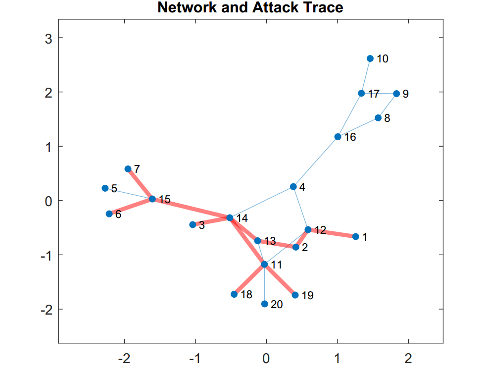
Figure 6 depicts a view of the network in MATLAB [6]. The red line indicates an example attack path, which enters through the wireless access point at node passes through the honeynet in nodes and and enters the SCADA components in nodes and The transitions are realized randomly.
Figure 7 depicts the cumulative utility of over time for five simulated attacks. Towards the beginning of the attacks, gains utility. But after learning nears completion (i.e., ), the losses from normal systems dominate. The filled boxes in each trace indicate the ejection point dictated by At these points, The ejection points are approximately at the maximum utility for traces and and obtain a positive utility in trace Trace involves a long period in which and sustains heavy losses. Since the traces are realized randomly, maximizes expected utility rather than realized utility.

VI Discussion of Results
This paper aimed to assess how long an intelligent network defender that detects an attacker should observe the attacker before ejecting him. We found that the defender should keep the attacker in a honeypot as long as information remains to be learned and in a normal system until a threshold amount of information remains. This threshold is at which the benefits of observation exactly balance the risks of information loss. Using this model, network designers can vary parameters (e.g., the number of honeypots and the rate at which they gather information) in order to maximize the value function In particular, we have examined the effect of the attacker move period using a Stackelberg game in which chooses the worst-case Future work can use signaling games to calculate attacker beliefs and based on defender strategies. Another direction, for distributed sensor-actuator networks, is to quantify the risk of system compromise using optimal control theory.
Appendix A Proof of Finite Expected Value
The maximum value of is achieved if only visits honeypots. In this case, so the expected utility is bounded from above. If chooses a poor policy (for example, for all and ), then can be unbounded below. On the other hand, can always guarantee (for example, by choosing for all and ). Therefore, the value of the optimal policy is bounded from below as well as from above.
Appendix B Derivation of Value Function and Optimal Policy
For the value function is piecewise-linear in Let denote restricted to the domain First, we find in terms of For any non-negative integer one step of the Bellman equation gives
where denotes achieves this maximization by continuing the game if the expected value for continuing is positive, and ejecting if the expected value is negative.
Rearranging terms and using Eq. (3-4) gives Now, we have defined as which makes the argument on the right side equal to zero. This obtains
Next, we find First, consider keeps in the honeypot until all residual utility is depleted, and then ejects him. Thus Next, for consider We have
A bit of algebra gives if and otherwise. Solving this recursive equation for the case of gives
| (9) |
Using initial condition produces for For consider the integer such that Then
But the last term is simply and defined in Eq. (5). Substituting from Eq. (9) gives the entire function
Appendix C Derivation of and
We solve first for and then for Because of the floor function in we have that Then for some
Appendix D Derivation of
We solve the value function in two cases.
D-A Limit as
As and decrease, so and the value functions follow Therefore, we find the limit of as As remains finite, but and approaches Therefore, the first two terms of approach zero. The last term expands to
As this approaches
| (11) |
Now, manipulation of Eq. (6) yields
But as the second term approaches zero. Thus approaches Eq. (11). We have proved Eq. (7).
D-B Large
There are several cases. First, consider and The second condition implies that keeps in the first honeypot that he enters until all residual utility is exhausted, which produces utility . The first condition implies that so which means that ejects from the first normal system that he enters, which produces utility. The weighted sum of these utilities gives Eq. (8).
Next, consider and The first condition implies that so it not guaranteed that But if ejects from the first normal system that he enters, and we have Eq. (8).
References
- [1] Massimiliano Albanese, Ermanno Battista, and Sushil Jajodia. Deceiving attackers by creating a virtual attack surface. In Cyber Deception, pages 169–201. Springer, 2016.
- [2] Devlin Barrett, Danny Yadron, and Damian Paletta. U.S. suspects hackers in China breached about 4 million people’s records, officials say. The Wall Street Journal, 2015. [Online] Available: https://www.wsj.com/.
- [3] Richard Bellman. On the theory of dynamic programming. Proc. Natl. Academy of Sciences, 38(8):716–719, 1952.
- [4] Thomas E Carroll and Daniel Grosu. A game theoretic investigation of deception in network security. Security and Communication Networks, 4(10):1162–1172, 2011.
- [5] Karel Durkota, Viliam Lisỳ, Branislav Bosanskỳ, and Christopher Kiekintveld. Optimal network security hardening using attack graph games. In Intl. Joint Conf. on Artificial Intelligence, pages 526–532, 2015.
- [6] MATLAB. R2017b. The MathWorks Inc., Natick, Massachusetts, 2017.
- [7] Keith W Miller, Jeffrey Voas, and George F Hurlburt. Byod: Security and privacy considerations. IT Professional, 14(5):53–55, 2012.
- [8] Mohammad A Noureddine, Ahmed Fawaz, William H Sanders, and Tamer Başar. A game-theoretic approach to respond to attacker lateral movement. In Decision and Game Theory for Security, pages 294–313. Springer, 2016.
- [9] United States Department of Defense. Department of Defense Strategy for Operating in Cyberspace. DIANE Publishing, 2012.
- [10] Jeffrey Pawlick, Sadegh Farhang, and Quanyan Zhu. Flip the cloud: Cyber-physical signaling games in the presence of advanced persistent threats. In Decision and Game Theory for Security, pages 289–308. Springer, 2015.
- [11] Jeffrey Pawlick and Quanyan Zhu. Deception by design: Evidence-based signaling games for network defense. In Workshop on the Economics of Inform. Security and Privacy, Delft, The Netherlands, 2015.
- [12] Jeffrey Pawlick and Quanyan Zhu. Strategic trust in cloud-enabled cyber-physical systems with an application to glucose control. IEEE Trans. Inform. Forensics and Security, 12(1), 2017.
- [13] Frank J. Stech, Kristin E. Heckman, and Blake E. Strom. Integrating cyber-D&D into adversary modeling for active cyber defense. In Cyber Deception, pages 169–201. Springer, 2016.
- [14] Chris Stokel-Walker. Hunting the DNC hackers: how Crowdstrike found proof Russia hacked the Democrats. WIRED, 2017. [Online] Available: http://www.wired.co.uk/.
- [15] M. van Dijk, A. Juels, A. Oprea, and R. L. Rivest. Flipit: The game of “stealthy takeover”. J Cryptology, 26(4):655–713, 2013.
- [16] Heinrich Von Stackelberg. Marktform und gleichgewicht. J. Springer, 1934.
- [17] J. Zhuang, V. M. Bier, and O. Alagoz. Modeling secrecy and deception in a multiple-period attacker–defender signaling game. European J Operational Res., 203(2):409–418, 2010.